Distribution Theory by Riemann Integrals

Abstract

It is the purpose of this article to outline a syllabus for a course that can be given to engineers looking for an understandable mathematical description of the foundations of distribution theory and the necessary functional analytic methods. Arguably, these are needed for a deeper understanding of basic questions in signal analysis. Objects such as the Dirac delta and the Dirac comb should have a proper definition, and it should be possible to explain how one can reconstruct a band-limited function from its samples by means of simple series expansions. It should also be useful for graduate mathematics students who want to see how functional analysis can help to understand fairly practical problems, or teachers who want to offer a course related to the “Mathematical Foundations of Signal Processing” at their institutions.
The course requires only an understanding of the basic terms from linear functional analysis, namely Banach spaces and their duals, bounded linear operators and a simple version of $w^{*}$-convergence. As a matter of fact we use a set of function spaces which is quite different from the collection of Lebesgue spaces $\big{(}{{{\bm{L}}^{p}}({\mathbb{R}}^{d})},\,\|\mbox{$\,\cdot\,$}\|_{p}\big{)}$ used normally. We thus avoid the use of Lebesgue integration theory. Furthermore we avoid topological vector spaces in the form of the Schwartz space.
Although practically all the tools developed and presented can be realized in the context of LCA (locally compact Abelian) groups, i.e. in the most general setting where a (commutative) Fourier transform makes sense, we restrict our attention in the current presentation to the Euclidean setting, where we have (generalized) functions over ${{{\mathbb{R}}^{d}}}$. This allows us to make use of simple BUPUs (bounded, uniform partitions of unity), to apply dilation operators and occasionally to make use of concrete special functions such as the (Fourier invariant) standard Gaussian, given by $g_{0}(t)=\exp(-\pi|t|^{2})$.
The problems of the overall current situation, with the separation of theoretical Fourier Analysis as carried out by (pure) mathematicians and Applied Fourier Analysis (as used in engineering applications) are getting bigger and bigger and therefore courses filling the gap are in strong need. This note provides an outline and may serve as a guideline. The first author has given similar courses over the last years at different schools (ETH Zürich, DTU Lyngby, TU Muenich, and currently Charlyes University Prague) and so one can claim that the outline is not just another theoretical contribution to the field.

1 Overall Motivation

1.1 Psychological Aspects

It is not a secret that the way how engineers or physicists are describing “realities” is quite different from the way mathematicians want to describe the same thing. The usual agreement is that applied scientists are motivated by the concrete applications and therefore do not need to be so pedantic in the description, because they have a “better feeling” about what is true and what is not true. After all, it does not pay to be too pedantic if one wants to make progress.

On the other hand mathematicians have a tendency to be too formal, to consider formal correctness of a statement as more important than the possible usefulness of a statement, simply because usefulness is not a category in mathematical sciences. Applicability by itself is not a criterion for important mathematical results which often go for the details of a structure without taking care of its relevance for applications. Sometimes this “abstract viewpoint” is very helpful, because it reveals important, underlying structures or allows to find connections between fields which appear to have very little in common at first sight. However, in the right (abstract) mathematical model they appear to be almost identical. Such observations allow to sometimes transfer information and insight, or computational rules established in one area to another area, which certainly is not possible if only one single application is in the focus.

There are different ways to view these discrepancies. What we could call the negative attitude is to say as a mathematician: You know, engineers and physicists are extremely sloppy, you never can trust their formulas. They claim to derive mathematical identities by using divergent integrals and so on, so one has to be careful in taking over what they “prove”. In the same way the engineer might say: You know, mathematicians are pedantic people who care only about technical details and not for the content of a formula. Whenever they claim that our formulas are not correct they find after some while a way to produce more theory in order to then prove that our formulas have been correct after all.

A more positive and ambitious approach would be to agree from both sides on a few facts which are on average quite valid:

• Any mathematical statement should, at least at the end, have a proper mathematical justification;

• Formulas developed from applied scientists may, at least at the beginning, come from intuition or experiments, so they might be valid under particular conditions or under implicit assumptions (which are often clear from the physical context, e.g. positivity assumptions, etc.);

• For the progress new formulas might be more important than a refined analysis of established formulas, but the goal is to have useful formulas whose range of applications (the relevant assumptions) are well understood; it is important to know when there is a guarantee that the formula can be applied (because there is a proof), and when one might be at risk of getting a wrong result (even if it is with low probability);

• This goal requires cooperation between applied scientists and mathematicians; usually the first group is better trained in establishing unexplored problems while the second is expected to provide a theoretical setup which ensures that things are under control, in terms of correctness of assumptions and conclusions. Obviously, in an ideal world one group can and should learn a lot from the other.

So in the cooperation between the two communities mathematicians should learn more about the goals and the motivation and e.g. engineers and physicists might learn that it is also beneficial to cooperate with mathematicians and to have clear guidelines concerning the correct use of formulas and mathematical identities and where perhaps caution is in place.

1.2 The search for a Banach space of test functions

The overall goal of this paper is to propose a path that allows us to introduce a family of generalized functions which is large enough to contain most of those generalized functions which are relevant in the context of (abstract or applied) Fourier analysis and for engineering applications. Specifically Dirac measures and Dirac combs. We will demonstrate that this is possible using modest tools from functional analysis.

Before going to the technical side of the exposition let us motivate the use of dual spaces and functional analytic methods, and shed some light on the idea of distributions. Let us start with some observations:

• First of all it is clear that generalized functions should form a linear space, so that linear combinations of those objects (sometimes called signals) can be formed, and under certain conditions, even limits, and hence infinite series;

• Secondly we would like to have “ordinary functions” included in a natural way within the world of generalized functions, so we need a natural embedding of as many linear spaces of ordinary functions as possible;

• As a third variant we can think of generalized functions as a kind of “limits” of ordinary functions, but in a specific sense (and ideally the convergence should also allowed to be applied to the generalized functions);

• Finally there are many operations that can be carried out for (certain) functions, such as translation, convolution, dilation, Fourier transform, and we will go for a setting where the approximation properties of the previous item allow to extend these operations to the linear space of generalized functions.

In order to explain our understanding of “distribution theory” let us first formulate again some general thoughts. In fact it is not surprising, that we have to use functional analytic methods in this context because after all at least for continuous variables signal spaces tend to be not finite-dimensional anymore and so we have to resort to methods that allow us to describe the convergence of infinite series. The simplest way to do this is to assume that one has a linear space and a normed space, $({\bm{B}},\,\|\mbox{$\,\cdot\,$}\|_{\bm{B}})$. If one has in addition a kind of multiplication $(a,b)\mapsto a\bullet b$ (with the usual rules) one speaks of normed algebras, if

$$\|b_{1}\bullet b_{2}\|_{\bm{B}}\leq\|b_{1}\|_{\bm{B}}\cdot\|b_{2}\|_{\bm{B}}\ \ \text{for all}\ \ b_{1},b_{2}\in{\bm{B}}.$$

Among the normed spaces those which are complete, the Banach spaces are the most important ones, because like ${\mathbb{R}}$ itself with the mapping $x\mapsto|x|$ one has (by definition) completeness, meaning that every Cauchy sequence is convergent. This is known to be equivalent to the fact that every absolutely convergent sequence with $\sum_{k=1}^{\infty}\|b_{k}\|_{\bm{B}}<\infty$, is convergent, so that the partial sums $\sum_{k=1}^{n}b_{k}$ have a limit (in $({\bm{B}},\,\|\mbox{$\,\cdot\,$}\|_{\bm{B}})$). Therefore the infinite sum is (unconditionally, or independent of the order) well defined, and thus the symbol $\sum_{k=1}^{\infty}b_{k}$ is meaningful in this situation.

The most important tool within linear functional analysis are the linear functionals, or bounded linear mappings from ${\bm{B}}$ into ${\mathbb{C}}$ (or into ${\mathbb{R}}$ for the case of real vector spaces). Such a functional $\sigma$ has to satisfy two properties:

1. Linearity: $\quad\sigma(\alpha{\bf b}_{1}+\beta{\bf b}_{2})=\alpha\sigma({\bf b}_{1})+\beta\sigma({\bf b}_{2}),\quad{\bf b}_{1},{\bf b}_{2}\in{\bm{B}},\alpha,\beta\in{\mathbb{C}}.$

2. Boundedness: There exists $c>0$ such that $\quad|\sigma({\bf b})|\leq C\|{\bf b}\|_{\bm{B}},\,\,\forall{\bf b}\in{\bm{B}}.$

For any given normed space $({\bm{B}},\,\|\mbox{$\,\cdot\,$}\|_{\bm{B}})$ the collection of all such bounded linear functionals constitutes the dual space, denoted by ${{\bm{B}}^{\prime}}$. It carries a norm, given by

$$\|\sigma\|_{{\bm{B}}^{\prime}}:=\sup_{\|{\bf b}\|_{\bm{B}}\leq 1}|\sigma({\bf b})|.$$

With this norm ${{\bm{B}}^{\prime}}$ turns out to be a Banach space. One can think of the dual space as the collection of all coordinate functionals (describing the contribution of a fixed element in a basis) over all finite dimensional subspaces of ${\bm{B}}$, thus capturing all the information about the underlying normed space.

In addition to norm convergence on ${{\bm{B}}^{\prime}}$ we will use what is called the $w^{*}$-convergence. It can be described for sequences as convergence in action:

For all practical purposes the following definition is a simple way of describing what is called $w^{*}$-convergence.

Definition 1.1.

A sequence of linear functionals $(\sigma_{n})_{n\geq 1}$ converges in action or in the weak^∗-sense to some $\sigma_{0}\in{{\bm{B}}^{\prime}}$ if we have

$$\lim_{n\to\infty}\sigma_{n}({\bf b})=\sigma_{0}({\bf b})\ \ \text{for all}\ \ {\bf b}\in{\bm{B}}.$$ (1)

By the Banach-Steinhaus Theorem the convergence for all ${\bf b}\in{\bm{B}}$ implies boundedness, i.e. $\sup_{n\geq 1}\|\sigma\|_{{\bm{B}}^{\prime}}<\infty,$ and that conversely it is (under this condition!) enough to claim that the limits on the left hand side exist for any ${\bf b}\in{\bm{B}}$, thus defining the functional $\sigma_{0}$. In fact, it would be even enough (given the boundedness condition) to know that one has a limit for all $b$ from a dense subspace of $({\bm{B}},\,\|\mbox{$\,\cdot\,$}\|_{\bm{B}})$.

Infinite dimensional Banach spaces $({\bm{B}},\,\|\mbox{$\,\cdot\,$}\|_{\bm{B}})$ do not satisfy the Heine-Borel property. A bounded sequence may fail to have a (norm) convergent subsequence. But the Banach-Alaoglou Theorem (see [8]) ensures that any bounded sequence $(\sigma_{k})$ in ${({{\bm{B}}^{\prime}},\|\mbox{$\,\cdot\,$}\|_{{\bm{B}}^{\prime}})}$ has a subsequence $(\sigma_{n_{k}})_{k\geq 1}$ which is $w^{*}$-convergent to some $\sigma_{0}\in{{\bm{B}}^{\prime}},$ i.e.

$$\lim_{k\to\infty}\sigma_{n_{k}}(b)=\sigma_{0}(b)\ \ \text{for all}\ \ {\bf b}\in{\bm{B}}.$$

In a similar way the set of all bounded and linear operators between two normed spaces is defined, we denote it by ${{\mathcal{L}}({{\bm{B}}^{1}}\negthinspace,\negthinspace{{\bm{B}}^{2}})}$. It is always a normed space with respect to the operator norm

$${|{\negthinspace\>\negthinspace}\|{T}|{\negthinspace\>\negthinspace}\|\,}:=\sup_{\|b_{1}\|_{{\bm{B}}^{1}}\leq 1}\|T(b_{1})\|_{{\bm{B}}^{2}}.$$

and if $({\bm{B}}^{2},\,\|\mbox{$\,\cdot\,$}\|^{(2)})$ is a Banach space the space of operators is complete as well. In particular, for the choice ${{\bm{B}}^{2}}={\mathbb{C}}$ the space reduces to the dual space.

For the case ${{\bm{B}}^{1}}={\bm{B}}={{\bm{B}}^{2}}$ these operators form a normed algebra, and in fact a Banach algebra if $({\bm{B}},\,\|\mbox{$\,\cdot\,$}\|_{\bm{B}})$ is a Banach space.

Since many sequences of functions which do not have a reasonable pointwise limit, such as a sequence of compressed box-functions which converge to the so-called Dirac Delta, often denoted by $\delta(t)$ in the engineering literature, are in fact limits in this sense, it is at least plausible to work with dual spaces in order to capture these limits.

Without going too much into the psychological and didactical side of this issue let us just state here that indeed, it is meaningful to model generalized functions as what we will call distributions, namely elements of dual spaces for suitable chosen Banach spaces $({\bm{B}},\,\|\mbox{$\,\cdot\,$}\|_{\bm{B}})$ of integrable and bounded, continuous functions.

We admit that of course this terminology is influenced by the existing traditional way of introducing generalized functions, e.g. by using the tempered distributions developed by Laurent Schwartz ([45]) using the (nuclear Frechet) space ${{\bm{\mathcal{S}}}({\mathbb{R}}^{d})}$ of rapidly descreasing functions. While differentiability is in the focus of attention there, we leave this aspect aside and allow ourselves to call an algebra (with respect to pointwise multiplication and/or convolution) of continuous functions a space of test functions and the dual space a space of distributions. This will be the setting we choose for our approach. Thus from now on we will mostly talk about test functions and distributions, but we will still have to explain in which sense distributions are generalized functions in the spirit of the above description.

One can also motivate the use of dual spaces for the description of linear spaces of signals by the following argument:

A signal is something that can be measured!

Just thinking of an audio signal which we can record using a microphone, we can compress using MP3 coding based on the FFT, and we can transmit it. All this is on the basis of linear measurements which are of course continuous in some sense, meaning that quite similar signals (whatever they are) will provide similar measurements. But is the audio signal a pointwise almost everywhere defined function in ${{{\bm{L}}^{2}}({\mathbb{R}})}$ in the mathematical sense? Of course we can take pictures of a natural scene and enjoy the quality of color picture taken by a $16$-million pixel camera, but does that device really sample (in the mathematical sense) a continuous, $2D$-function describing the analog picture which we use in a conversational situation?

The situation is really much more like an abstract probability distribution, say a normal distribution with some expectation value and some variance. We will never be able (except through indirect mathematical description) to provide a pointwise description of such a “distribution” (a different but related use of this word), so normally one resorts to the use of histograms. Given the bins used for the histogram one can describe the height of the bars simply as the value obtained by applying the (non-negative) measure (via integration) to the indicator function of the corresponding interval (bin), making sure that the union of the bins is the whole real line or at least the range of the random variable resp. the support of the corresponding measure.

What we are doing here is essentially to replace those (finer and finer) bins by BUPUs (uniform partitions of unity), with the extra demand of assuming that they are continuous and not just step functions. The reader should see this as a minor and just technical modification (which is avoiding the distinction between step functions and continuous functions, and is also much more convenient for the setting of LCA groups).

The (abstract) viewpoint of considering signals as something that can be measured also suggests very naturally a measure of similarity of signals. If for a given (potentially comprehensive) set of measurements only very small deviations are observed, then we think of those signals as “quite similar”, and a sequence of signals may converge in this way to a limit signal (e.g. coarse approximations to the continuous limit). But this kind of convergence is encapsulated mathematically in the concept of $w^{*}$-convergence described above, that will be used intensively in this text.

2 Notations and Preliminaries

Although the approach described below can be used to develop Harmonic Analysis in the context of locally compact Abelian (LCA) groups we restrict our attention to the setting of Euclidean spaces ${{{\mathbb{R}}^{d}}}$. This is the framework relevant for most engineering work and physics.

Let us fix some notation. It all starts with the most simple vector space of functions on ${{{\mathbb{R}}^{d}}}$, namely ${{{\bm{C}}_{\negthinspace c}}({\mathbb{R}}^{d})}$, the space of continuous, complex-valued and compactly supported functions on ${{{\mathbb{R}}^{d}}}$, i.e. with $\operatorname{supp}(k)\subset B_{R}(0):=\{x\,:\,|x|\leq R\}$ for some $R>0$. For such a function $f\in{{{\bm{C}}_{\negthinspace c}}({\mathbb{R}}^{d})}$ the notion of an integral, $\int_{{\mathbb{R}}^{d}}f(t)\,dt$, is well-defined by Riemann integration, and thus this (infinite-dimensional) linear space of functions can be endowed with many different norms, such as the maximum-norm or uniform-norm, $\|k\|_{\infty}=\sup_{t\in{{{\mathbb{R}}^{d}}}}|f(t)|$ and the $p$-norms $\|k\|_{p}=(\int_{{\mathbb{R}}^{d}}|k(t)|^{p}\,dt)^{1/p}$ for $1\leq p<\infty$. The completion of ${{{\bm{C}}_{\negthinspace c}}({\mathbb{R}}^{d})}$ with respect to the $p$-norm yields the Lebesgue spaces, $\big{(}{{{\bm{L}}^{p}}({\mathbb{R}}^{d})},\,\|\mbox{$\,\cdot\,$}\|_{p}\big{)}$. Most notably are ${{{\bm{L}}^{1}}({\mathbb{R}}^{d})}$ and ${{{\bm{L}}^{2}}({\mathbb{R}}^{d})}$. The latter being a Hilbert space with respect to the inner-product $\langle f,g\rangle=\int_{{\mathbb{R}}^{d}}f(t)\,\overline{g(t)}\,dt$.

For complex-valued functions $f,g$ on ${{{\mathbb{R}}^{d}}}$ we define the following operations,

1. point-wise multiplication, $(f\cdot g)(t)=f(t)\cdot g(t)$, $t\in{{{\mathbb{R}}^{d}}}$,

2. flip operation, $f^{\checkmark}\!(t)=f(-t)$,

3. complex conjugation, $\overline{f}(t)=\overline{f(t)}$,

4. translation by $x\in{{{\mathbb{R}}^{d}}}$, $T_{x}f(t)=f(t-x)$,

5. modulation by $\omega\in{{{\mathbb{R}}^{d}}}$, $E_{\omega}f(t)=e^{2\pi i\omega\cdot t}\,f(t)$,

6. dilation by an invertible $d\times d$ matrix $A$, $\alpha_{A}f(t)=|\det(A)|^{1/2}\,f(At)$,

7. specifically homogeneous dilations for $\rho>0$,
   $\quad[{\operatorname{St}_{\rho}}f](t)=\rho^{-d}f(t/\rho),$ and $[{\operatorname{D}_{\rho}}h](t)=h(\rho t)$
   with $\|{\operatorname{St}_{\rho}}f\|_{1}=\|f\|_{1}$ and $\|{\operatorname{D}_{\rho}}f\|_{\infty}=\|f\|_{\infty}.$

Let $\Delta$ be the tent-function given by

$$\Delta(t)=\prod_{j=1}^{d}\max\big{(}1-2|t^{(j)}|,0\big{)},\ \ t=(t^{(1)},t^{(2)},\ldots,t^{(d)})\in{{{\mathbb{R}}^{d}}}.$$

Observe that $\operatorname{supp}\,\Delta=[-1/2,1/2]^{d}$. We define the family of functions $(\psi_{n})_{n\in\mathbb{Z}^{d}}$ to be the collection of half-integer translates of $\Delta$, so that

$$\psi_{n}(t)=\Delta\big{(}t-\tfrac{1}{2}n\big{)},\ t\in{{{\mathbb{R}}^{d}}},\ n\in\mathbb{Z}^{d}.$$ (2)

The crucial properties of the functions $(\psi_{n})$ are for us that they satisfy the general assumptions of a bounded uniform partition of unity (BUPU), of which we give the definition below. Throughout this work $(\psi_{n})$ will always refer to the functions in (2). However, any other BUPU can also be used, which entails only minor modifications to our proofs.

For most applications regular BUPUs will be sufficient (and easier to handle), which are obtained as translates of one (smooth) function with compact support along some lattice in ${{{\mathbb{R}}^{d}}}$. In this setting it is natural to use smooth BUPUs with respect to some lattice $\Lambda={\bf A}{{\mathbb{Z}}^{d}}$, for some non-singular $d\times d$ matrix ${\bf A}$. For convenience of notation we use mostly lattices of the form $\gamma{{\mathbb{Z}}^{d}}$, for some $\gamma>0$.

Definition 2.1.

A family $\Psi=(\psi_{k})_{k\in{{\mathbb{Z}}^{d}}}=(T_{\gamma k}\psi_{0})_{k\in{{\mathbb{Z}}^{d}}}$ in ${{{\bm{C}}_{\negthinspace c}}({\mathbb{R}}^{d})}$ (for some $\gamma>0$) is called a regular, uniform partition of unity on ${{{\mathbb{R}}^{d}}}$ of size $R$, (we write $|\Psi|\leq R$ or $\operatorname{diam}{\Psi}\leq R$) if

1. $\psi_{0}$ is compactly supported in $B_{R}(0)$.

2. $\sum_{k\in{{\mathbb{Z}}^{d}}}\psi_{k}(x)=\sum_{k\in{{\mathbb{Z}}^{d}}}\psi_{0}(x-\gamma k)\equiv 1$ on ${{{\mathbb{R}}^{d}}}$.

Usually it is assumed that $\psi_{0}(x)\geq 0$.

3 Continuous functions that vanish at infinity

The uniform or sup-norm of functions on ${{{\mathbb{R}}^{d}}}$ is defined by $\|f\|_{\infty}=\sup_{t\in{{{\mathbb{R}}^{d}}}}|f(t)|.$

Observe that ${{{\bm{C}}_{\negthinspace b}}({{{\mathbb{R}}^{d}}})}$, the space of all bounded, continuous, complex-valued functions on ${{{\mathbb{R}}^{d}}}$ is a Banach algebra with respect to this norm and pointwise multiplication. It is easy to show that $({{{\bm{C}}_{\negthinspace c}}({\mathbb{R}}^{d})},\|\,\cdot\,\|_{\infty})$ is not complete. Its completion in ${\big{(}{{\bm{C}}_{\negthinspace b}}({\mathbb{R}}^{d}),\,\|\mbox{$\,\cdot\,$}\|_{\infty}\big{)}}$, which is the same as the closure within ${\big{(}{{\bm{C}}_{\negthinspace b}}({\mathbb{R}}^{d}),\,\|\mbox{$\,\cdot\,$}\|_{\infty}\big{)}}$, is just the space of continuous functions that vanish at infinity. We denote this space by ${\big{(}{{\bm{C}}_{\negthinspace 0}}({\mathbb{R}}^{d}),\,\|\mbox{$\,\cdot\,$}\|_{\infty}\big{)}}$. For $f\in{{{\bm{C}}_{\negthinspace 0}}({\mathbb{R}}^{d})}$ and $h\in{{{\bm{C}}_{\negthinspace b}}({{{\mathbb{R}}^{d}}})}$ the pointwise product $f\cdot h$ is again in ${{{\bm{C}}_{\negthinspace 0}}({\mathbb{R}}^{d})}$. In particular, ${\big{(}{{\bm{C}}_{\negthinspace 0}}({\mathbb{R}}^{d}),\,\|\mbox{$\,\cdot\,$}\|_{\infty}\big{)}}$ is itself a (commutative) Banach algebra with respect to pointwise multiplication, with

$$\|f\cdot h\|_{\infty}\leq\|f\|_{\infty}\,\|h\|_{\infty}.$$ (3)

We define the space of bounded measures ${{{\bm{M}}_{\negthinspace b}}({\mathbb{R}}^{d})}$ to be the continuous (Banach space) dual of ${\big{(}{{\bm{C}}_{\negthinspace 0}}({\mathbb{R}}^{d}),\,\|\mbox{$\,\cdot\,$}\|_{\infty}\big{)}}$. That is, ${{{\bm{M}}_{\negthinspace b}}({\mathbb{R}}^{d})}={{{\bm{C}}^{\prime}_{\negthinspace 0}}({\mathbb{R}}^{d})}$ consists of all linear and continuous functionals $\mu:{{{\bm{C}}_{\negthinspace 0}}({\mathbb{R}}^{d})}\to\mathbb{C}$. We write the action of a functional $\mu\in{{{\bm{M}}_{\negthinspace b}}({\mathbb{R}}^{d})}$ on a function $f\in{{{\bm{C}}_{\negthinspace 0}}({\mathbb{R}}^{d})}$ as $\mu(f)$. Naturally, ${{{\bm{M}}_{\negthinspace b}}({\mathbb{R}}^{d})}$ is a Banach space with respect to the operator norm,

$$\|\mu\|_{{{\bm{M}}_{\negthinspace b}}}=\sup_{{f\in{{{\bm{C}}_{\negthinspace 0}}({\mathbb{R}}^{d})},\,\,\|f\|_{\infty}\leq 1}}\big{|}\mu(f)\big{|}.$$ (4)

There are two simple and natural examples of bounded measures. First of all the Dirac measure (or Dirac delta) of the form $\delta_{x}:f\mapsto f(x)$, $x\in{{{\mathbb{R}}^{d}}}$. Their finite linear combinations are called finite discrete measures and belong also to ${{{\bm{M}}_{\negthinspace b}}({\mathbb{R}}^{d})}$.

Secondly, any function $g\in{{{\bm{C}}_{\negthinspace c}}({\mathbb{R}}^{d})}$ defines a bounded measure $\mu_{g}$ by

$$\mu_{g}:{{{\bm{C}}_{\negthinspace 0}}({\mathbb{R}}^{d})}\to\mathbb{C},\quad\mu_{g}(f)=\int_{{\mathbb{R}}^{d}}f(t)\,g(t)\,dt,\ \ f\in{{{\bm{C}}_{\negthinspace 0}}({\mathbb{R}}^{d})}.$$ (5)

This integral is well defined as $f\cdot g\in{{{\bm{C}}_{\negthinspace c}}({\mathbb{R}}^{d})}$.

We mention the following operations that one can do with bounded measures: we define the product of a bounded measure $\mu\in{{{\bm{M}}_{\negthinspace b}}({\mathbb{R}}^{d})}$ with a function $h\in{{{\bm{C}}_{\negthinspace b}}({{{\mathbb{R}}^{d}}})}$ to be the bounded measure given by

$$\big{(}\mu\cdot h\big{)}(f):=\mu(h\cdot f)\ \ \text{for all}\ \ f\in{{{\bm{C}}_{\negthinspace 0}}({\mathbb{R}}^{d})}.$$ (6)

Observe that $\|\mu\cdot h\|_{{{\bm{M}}_{\negthinspace b}}}\leq\|h\|_{\infty}\,\|\mu\|_{{{\bm{M}}_{\negthinspace b}}},$ and of course associativity.

Furthermore, we define the complex conjugation of a bounded measure, its flip, translation, modulation and dilation to be, for any $\mu\in{{{\bm{M}}_{\negthinspace b}}({\mathbb{R}}^{d})}$ and $f\in{{{\bm{C}}_{\negthinspace 0}}({\mathbb{R}}^{d})}$,

$$\overline{\mu}(f) =\overline{\mu(\overline{f})},$$

$$\mu^{\checkmark}\!(f) =\mu(f^{\checkmark}\!),$$

$$\big{(}T_{x}\mu\big{)}(f) =\mu(T_{-x}f),\ x\in{{{\mathbb{R}}^{d}}},$$

$$\big{(}E_{\omega}\mu\big{)}(f) =\mu(E_{\omega}f),\ \omega\in{{{\mathbb{R}}^{d}}},$$

$$\big{(}\alpha_{A}\mu)(f) =\mu(\alpha_{A^{-1}}f),\ A\in\textnormal{GL}_{\mathbb{R}}(d).$$

The reader may verify consistency with the corresponding operators defined on ordinary functions, i.e. that for any $g\in{{{\bm{C}}_{\negthinspace c}}({\mathbb{R}}^{d})}$

$$\overline{\mu_{g}}=\mu_{\overline{g}},\ \ (\mu_{g})^{\checkmark}\!=\mu_{g^{\checkmark}},\ \ T_{x}\mu_{g}=\mu_{T_{x}g},\ \ E_{\omega}\mu_{g}=\mu_{E_{\omega}g},\ \ \alpha_{A}\mu_{g}=\mu_{\alpha_{A}g}.$$

Furthermore, one has the following rather natural rules:

$$T_{y}\delta_{x}=\delta_{x+y},\ \ \delta_{x}^{\checkmark}=\delta_{-x},\ \ \overline{\delta_{x}}=\delta_{x},\ \ \delta_{x}\cdot h=h(x)\cdot\delta_{x}.$$

Finally we define $\mu*f$ to be the convolution of a function $f\in{{{\bm{C}}_{\negthinspace 0}}({\mathbb{R}}^{d})}$ with a measure $\mu\in{{{\bm{M}}_{\negthinspace b}}({\mathbb{R}}^{d})}$. It is a new function on ${{{\mathbb{R}}^{d}}}$ given pointwise by

$$\big{(}\mu*f\big{)}(x)=\mu(T_{x}[f^{\checkmark}])=\big{(}T_{-x}\mu\big{)}(f^{\checkmark}\!),\ \ x\in{{{\mathbb{R}}^{d}}}.$$ (7)

Observe that $\delta_{x}*f=T_{x}f$. This correspondence is in fact the reason why the “moving average” described in (7) makes use of the flip-operator.

Theorem 3.1.

For any $\mu\in{{{\bm{M}}_{\negthinspace b}}({\mathbb{R}}^{d})}$ and any $f\in{{{\bm{C}}_{\negthinspace 0}}({\mathbb{R}}^{d})}$ the convolution product $\mu*f$ is a function in ${{{\bm{C}}_{\negthinspace 0}}({\mathbb{R}}^{d})}$. Moreover, $C_{\mu}:f\mapsto\mu\ast f$ is a bounded operator

$$\|\mu*f\|_{\infty}\leq\|\mu\|_{{{\bm{M}}_{\negthinspace b}}}\,\|f\|_{\infty},\quad f\in{{{\bm{C}}_{\negthinspace 0}}({\mathbb{R}}^{d})},$$

which commutes with translations, i.e. $\mu\ast(T_{x}f)=T_{x}(\mu\ast f)$ for all $x\in{{{\mathbb{R}}^{d}}}$. Moreover, the operator norm of $C_{\mu}$ equals the functional norm of $\mu$.

One can in fact show that every continuous operator $T:{{{\bm{C}}_{\negthinspace 0}}({\mathbb{R}}^{d})}\to{{{\bm{C}}_{\negthinspace 0}}({\mathbb{R}}^{d})}$ that satisfied the commutation relation $T\circ T_{x}=T_{x}\circ T$ for all $x\in{{{\mathbb{R}}^{d}}}$ is given by an operator that convolves with some uniquely determined measure $\mu\in{{{\bm{C}}_{\negthinspace b}}({{{\mathbb{R}}^{d}}})}$. A proof of this statement and Theorem 3.1 can be found in the first author’s lecture notes. Such an operator is also called a translation invariant linear system (TILS). For more on this, see Section 11.

Definition 3.2.

Given $f\in{{{\bm{C}}_{\negthinspace b}}({{{\mathbb{R}}^{d}}})}$ and $\delta>0$ we define the oscillation function

$$\operatorname{osc}_{\delta}(f){{{\raise 0.5pt\hbox{\footnotesize$($}}}{x}{{\raise 0.5pt\hbox{\footnotesize$)$}}}}:=\max_{|y|\leq\delta}|f(x)-f(x+y)|.$$ (8)

We also define the local maximal function for any $f\in{{{\bm{C}}_{\negthinspace b}}({{{\mathbb{R}}^{d}}})}$,

$$f^{\#}(x)=\max_{|y|\leq 1}|f(x+y)|,\quad x\in{{{\mathbb{R}}^{d}}}.$$ (9)

There are a couple of harmless but useful pointwise estimates:

Lemma 3.3.

For any two functions $f,f_{1},f_{2}\in{{{\bm{C}}_{\negthinspace b}}({{{\mathbb{R}}^{d}}})}$ one has that

1. $\operatorname{osc}_{\delta}(f)\leq 2f^{\#}$;

2. $\operatorname{osc}_{\delta}(f_{1}+f_{2})\leq\operatorname{osc}_{\delta}(f_{1})+\operatorname{osc}_{\delta}(f_{2});$

3. $|f|\leq|g|\Rightarrow f^{\#}\leq g^{\#};$

4. $(f_{1}+f_{2})^{\#}\leq f_{1}^{\#}+f_{2}^{\#};$

5. $\operatorname{osc}_{\delta}(T_{x}f)=T_{x}\operatorname{osc}_{\delta}(f);$

6. $(T_{x}f)^{\#}=T_{x}(f^{\#}).$

Proof.

The proof is left as an exercise to the reader. ∎

Using these relations, the following is a simple observation.

Lemma 3.4.

A function $f\in{{{\bm{C}}_{\negthinspace b}}({{{\mathbb{R}}^{d}}})}$ is uniformly continuous if and only if

$${\lVert\operatorname{osc}_{\delta}(f)\rVert_{\infty}}\to 0\ \ \text{for}\ \ \delta\to 0.$$

For every BUPU $\Psi$ we define the spline-type quasi interpolation operator

$$f\mapsto\operatorname{Sp}_{\Psi}f:\quad\operatorname{Sp}_{\Psi}f(t)=\sum_{n\in\mathbb{Z}^{d}}f(t_{n})\psi_{n}(t),\ \ t\in{{{\mathbb{R}}^{d}}}.$$ (10)

Lemma 3.5.

For any regular BUPU $\Psi$ the operator $\operatorname{Sp}_{\Psi}$ maps ${{{\bm{C}}_{\negthinspace 0}}({\mathbb{R}}^{d})}$ and ${{{\bm{C}}_{\negthinspace b}}({{{\mathbb{R}}^{d}}})}$ onto itself, respectively, with $\|\operatorname{Sp}_{\Psi}f\|_{\infty}\leq\|f\|_{\infty}.$ One has $\|\operatorname{Sp}_{\Psi}f-f\|_{\infty}\to 0$ as $\operatorname{diam}(\Psi)\to 0$ if and only if $f$ is uniformly continuous (e.g. $f\in{{{\bm{C}}_{\negthinspace 0}}({\mathbb{R}}^{d})}$).

Proof.

The first statement follows easily from the fact that all $\psi_{n}$ are continuous and compactly supported together with the assumed properties of the function $f$. For the second statement note that we only have to do a pointwise estimate between $f(t)$ and $\operatorname{Sp}_{\Psi}f(t)=\sum_{n\in{{\mathbb{Z}}^{d}}}\psi_{n}(t_{n})f(t)$, where $I\subset\mathbb{Z}^{d}$ is such that $\operatorname{supp}\,\psi_{n}\cap B_{\delta}(t)\neq\emptyset$ for all $n\in{{\mathbb{Z}}^{d}}$. Using the fact that the $(\psi_{n})$ form a partition of unity, we establish that

$$|\operatorname{Sp}_{\Psi}f(t)-f(t)| \leq\sum_{n\in{{\mathbb{Z}}^{d}}}|f(t_{n})-f(t)|\cdot\psi_{n}(t)$$

If $\Psi$ is a BUPU such that $|t-t_{n}|\leq\delta$ for all $t\in\operatorname{supp}(\psi_{n})$, then we find that

$$|\operatorname{Sp}_{\Psi}f(t)-f(t)|\leq\operatorname{osc}_{\delta}(f)(t).$$

As the support of the functions in the BUPU $\Psi$ is made smaller, we write $|\Psi|\to 0$, $\delta$ go to zero. By Lemma 3.4 we conclude that $\|\operatorname{Sp}_{\Psi}f-f\|_{\infty}\to 0$ as $|K|\to 0$.∎

One important result that we need for later is the following one. We give a proof of Theorem 3.6 at the end of this section.

Theorem 3.6.

Let $\Psi=(\psi_{n})_{n\in\mathbb{Z}^{d}}$ be the BUPU as in (2). Every $\mu\in{{{\bm{M}}_{\negthinspace b}}({\mathbb{R}}^{d})}$ can be represented by the absolutely norm convergent series $\mu=\sum_{n\in\mathbb{Z}^{d}}\mu\cdot\psi_{n}$. Moreover,

$$\|\mu\|_{{{\bm{M}}_{\negthinspace b}}}=\sum_{n\in\mathbb{Z}^{d}}\|\mu\cdot\psi_{n}\|_{{{\bm{M}}_{\negthinspace b}}}.$$ (11)

Corollary 3.7.

For any $\mu\in{{{\bm{M}}_{\negthinspace b}}({\mathbb{R}}^{d})}$ and any $\varepsilon>0$ there exists a finite subset $F_{0}\subset\mathbb{Z}^{d}$ such that $\|\mu-\sum_{n\in F}\mu\cdot\psi_{n}\|_{{{\bm{M}}_{\negthinspace b}}}<\varepsilon$ for any finite subset of ${{\mathbb{Z}}^{d}}$ with $F\supseteq F_{0}$. One can think of $p=\sum_{n\in F}\psi_{n}\in{{{\bm{C}}_{\negthinspace c}}({\mathbb{R}}^{d})}$ as a plateau-type function with $\|\mu-\mu\cdot p\|_{{{\bm{M}}_{\negthinspace b}}}<\varepsilon$.

Proof of Theorem 3.6. For any given ${\varepsilon>0}$ let $\varepsilon_{n}>0$, $n\in\mathbb{Z}^{d}$ be such that $\sum_{n\in\mathbb{Z}^{d}}\varepsilon_{n}<\varepsilon$. By the definition of $\|\mu\cdot\psi_{n}\|_{{{\bm{M}}_{\negthinspace b}}}$ we can find $f_{n}\in{{{\bm{C}}_{\negthinspace 0}}({\mathbb{R}}^{d})}$, $\|f_{n}\|_{\infty}\leq 1$ such that

$$|\big{(}\mu\cdot\psi_{n}\big{)}(f_{n})|>\|\mu\cdot\psi_{n}\|_{{{\bm{M}}_{\negthinspace b}}}-\varepsilon_{n}.$$

Without loss of generality, we can assume that $\big{(}\mu\cdot\psi_{n}\big{)}(f_{n})$ is real-valued and non-negative. For any finite set $F\subset\mathbb{Z}^{d}$ we define $f\in{{{\bm{C}}_{\negthinspace c}}({\mathbb{R}}^{d})}$ by $f=\sum_{n\in F}f_{n}\cdot\psi_{n}$. We now observe that

$$\mu(f) =\sum_{n\in F}\mu(f_{n}\cdot\psi_{n})=\sum_{n\in F}\big{(}\mu\cdot\psi_{n}\big{)}(f_{n})$$

$$>\sum_{n\in F}\big{(}\|\mu\cdot\psi_{n}\|_{{{\bm{M}}_{\negthinspace b}}}-\varepsilon_{n}\big{)}>\Big{(}\sum_{n\in F}\|\mu\cdot\psi_{n}\|_{{{\bm{M}}_{\negthinspace b}}}\Big{)}-\varepsilon.$$

By a simple pointwise estimate we find that $\|f\|_{\infty}\leq 1$. Thus that for every $\varepsilon>0$ and any finite set $F\subset\mathbb{Z}^{d}$ there is a function $f\in{{\bm{C}}_{\negthinspace c}}({{{\mathbb{R}}^{d}}})$, $\|f\|_{\infty}\leq 1$, such that

$$\sum_{n\in F}\|\mu\cdot\psi_{n}\|_{{{\bm{M}}_{\negthinspace b}}}\leq\mu(f)+\varepsilon$$

This being true for any ${\varepsilon>0}$ and any finite set we conclude that

$$\sum_{n\in{{\mathbb{Z}}^{d}}}\|\mu\cdot\psi_{n}\|_{{{\bm{M}}_{\negthinspace b}}}\leq\|\mu\|_{{{\bm{M}}_{\negthinspace b}}}.$$

Hence $\sum_{n\in\mathbb{Z}^{d}}\mu\cdot\psi_{n}$ is absolutely convergent in ${{{\bm{M}}_{\negthinspace b}}({\mathbb{R}}^{d})}$. Finally we show that $\mu=\sum_{n\in\mathbb{Z}^{d}}\mu\cdot\psi_{n}$. For any $f\in{{{\bm{C}}_{\negthinspace c}}({\mathbb{R}}^{d})}$ we clearly have

$$\Big{(}\sum_{n\in\mathbb{Z}^{d}}\mu\cdot\psi_{n}\Big{)}(f)=\sum_{n\in F}\big{(}\mu\cdot\psi_{n})(f)=\mu\big{(}\sum_{n\in F}\psi_{n}\cdot f\big{)}=\mu(f),$$

where $F$ is some finite subset of $\mathbb{Z}^{d}$ that depends on the support of $f$. Since this equality holds for all ${{{\bm{C}}_{\negthinspace c}}({\mathbb{R}}^{d})}$ which is dense in ${{{\bm{C}}_{\negthinspace 0}}({\mathbb{R}}^{d})}$, we get $\mu=\sum_{n\in\mathbb{Z}^{d}}\mu\cdot\psi_{n}$. The opposite estimate, namely $\|\mu\|_{{{\bm{M}}_{\negthinspace b}}}\leq\sum_{n\in\mathbb{Z}^{d}}\|\mu\cdot\psi_{n}\|_{{{\bm{M}}_{\negthinspace b}}}$ is clear by the triangle inequality and the completeness of ${({{\bm{M}}_{\negthinspace b}}({\mathbb{R}}^{d}),\|\mbox{$\,\cdot\,$}\|_{{\bm{M}}_{\negthinspace b}})}$.

4 The Wiener Algebra on ${{{\mathbb{R}}^{d}}}$

At this point we are in a situation where we can define pointwise multiplication within the Banach algebra ${\big{(}{{\bm{C}}_{\negthinspace 0}}({\mathbb{R}}^{d}),\,\|\mbox{$\,\cdot\,$}\|_{\infty}\big{)}}$ and we can convolve a measure with a function ${{{\bm{C}}_{\negthinspace 0}}({\mathbb{R}}^{d})}$. Furthermore, we can multiply any measure with a function in ${{{\bm{C}}_{\negthinspace b}}({{{\mathbb{R}}^{d}}})}$, always together with the corresponding norm estimates.

But not every function $f\in{{{\bm{C}}_{\negthinspace 0}}({\mathbb{R}}^{d})}$ defines a measure and it is not possible to define the convolution product of two arbitrary functions $f_{1},f_{2}\in{{{\bm{C}}_{\negthinspace 0}}({\mathbb{R}}^{d})}$. Hence it is desirable to reduce the reservoir of “test functions” from ${\big{(}{{\bm{C}}_{\negthinspace 0}}({\mathbb{R}}^{d}),\,\|\mbox{$\,\cdot\,$}\|_{\infty}\big{)}}$ to a smaller one. The first step into this direction will be the introduction of “our new space of test functions”, the Wiener algebra. It is defined as follows:

Definition 4.1.

Given the BUPU $\Psi=(\psi_{n})_{n\in{{\mathbb{Z}}^{d}}}$ in (2) the Wiener algebra ${\bm{W}}({{{\mathbb{R}}^{d}}})$ consist of all continuous functions $f\in{{{\bm{C}}_{\negthinspace b}}({{{\mathbb{R}}^{d}}})}$ for which the following norm is finite:

$$\|f\|_{\bm{W}}:=\sum_{n\in{{\mathbb{Z}}^{d}}}\|f\cdot\psi_{n}\|_{\infty}<\infty.$$ (12)

One can show that the definition does not depend on the particular choice of the BUPU, i.e. different BUPUs $\Psi^{1}$ or $\Psi^{2}$ define the same space. Also, ${({{\bm{W}}({{{\mathbb{R}}^{d}}})},\|\mbox{$\,\cdot\,$}\|_{\bm{W}})}$ is a Banach space. We mention that an equivalent norm on ${{\bm{W}}({{{\mathbb{R}}^{d}}})}$ is given by

$$\|f\|_{{\bm{W}},\,\sqcap}=\sum_{n\in\mathbb{Z}^{d}}\|f\cdot T_{n}\mathds{1}_{[0,1]^{d}}\|_{\infty},$$

where $\mathds{1}_{[0,1]^{d}}$ is the characteristic function on the set $[0,1]^{d}$. This is the norm still widely used in the literature, and used in H. Reiter’s book [38] as an example of an interesting Segal algebra (and even going back to N. Wiener’s work on Tauberian theorems). Convolution relations for this (and more general Wiener amalgam spaces) are given in [6, 16] and [29].

Observe that for any $f\in{{\bm{W}}({{{\mathbb{R}}^{d}}})}$ and $x\in{{{\mathbb{R}}^{d}}}$ we have, in general, that $\|T_{x}f\|_{{\bm{W}}}\neq\|f\|_{{\bm{W}}}$. We will not need a norm that is strictly isometric with respect to translation. One way to do this is to introduce the continuous description of amalgam norms, which has been given already in [11].

The Wiener algebra relates to the previously considered function spaces as follows: All functions in ${{\bm{W}}({{{\mathbb{R}}^{d}}})}$ belong to ${{{\bm{C}}_{\negthinspace 0}}({\mathbb{R}}^{d})}$. The space ${{{\bm{C}}_{\negthinspace c}}({\mathbb{R}}^{d})}$ is contained in ${({{\bm{W}}({{{\mathbb{R}}^{d}}})},\|\mbox{$\,\cdot\,$}\|_{\bm{W}})}$ and ${{\bm{W}}({{{\mathbb{R}}^{d}}})}$ is contained in ${\big{(}{{\bm{C}}_{\negthinspace 0}}({\mathbb{R}}^{d}),\,\|\mbox{$\,\cdot\,$}\|_{\infty}\big{)}}$, both as dense subspaces. All the inclusions are in fact continuous embeddings. Furthermore, just as ${{{\bm{C}}_{\negthinspace 0}}({\mathbb{R}}^{d})}$ and ${{{\bm{C}}_{\negthinspace b}}({{{\mathbb{R}}^{d}}})}$, the Wiener algebra behaves well with respect to multiplication.

Lemma 4.2.

1. The Wiener algebra ${\bm{W}}({{{{\mathbb{R}}^{d}}}})$ is continuously embedded into ${{{\bm{C}}_{\negthinspace b}}({{{\mathbb{R}}^{d}}})}$ and ${{{\bm{C}}_{\negthinspace 0}}({\mathbb{R}}^{d})}$. Specifically, one has that

   $$\|f\|_{\infty}\leq\|f\|_{{\bm{W}}}\ \ \text{for all}\ \ f\in{\bm{W}}({{{\mathbb{R}}^{d}}}).$$

2. The Wiener algebra is an ideal of ${{{\bm{C}}_{\negthinspace b}}({{{\mathbb{R}}^{d}}})}$ with respect to pointwise multiplication. In fact, for any $h\in{{{\bm{C}}_{\negthinspace b}}({{{\mathbb{R}}^{d}}})}$ and $f\in{\bm{W}}({{{\mathbb{R}}^{d}}})$ one has that

   $$\|h\cdot f\|_{{\bm{W}}}\leq\|h\|_{\infty}\,\|f\|_{{\bm{W}}}.$$

3. The Wiener algebra is a Banach algebra with respect to pointwise multiplication. For any $f,h\in{\bm{W}}({{{\mathbb{R}}^{d}}})$ we have that $\|h\cdot f\|_{{\bm{W}}}\leq\|h\|_{{\bm{W}}}\,\|f\|_{{\bm{W}}}$.

Proof.

(i). By assumption we have $1=\sum_{n\in\mathbb{Z}^{d}}\psi_{n}(x)$ for all $x\in{{{\mathbb{R}}^{d}}}$. Hence

$$\sup_{x\in{{{\mathbb{R}}^{d}}}}|f(x)|=\sup_{x\in{{{\mathbb{R}}^{d}}}}|\sum_{n\in\mathbb{Z}^{d}}f(x)\,\psi_{n}(x)|\leq\sum_{n\in\mathbb{Z}^{n}}\|f\cdot\psi_{n}\|_{\infty}=\|f\|_{{\bm{W}}}<\infty,\quad\forall f\in{\bm{W}}({{{\mathbb{R}}^{d}}}).$$

(ii). Let $h$ and $f$ be as in the statement. It follows from the easy estimate

$$\sum_{n\in\mathbb{Z}^{d}}\|h\cdot f\cdot\psi_{n}\|_{\infty}\leq\|h\|_{\infty}\,\sum_{n\in\mathbb{Z}^{d}}\|f\cdot\psi_{n}\|_{\infty}=\|h\|_{\infty}\,\|f\|_{{\bm{W}}}.$$

(iii). This follows by (i) and (ii). ∎

Lemma 4.3.

The translation and the modulation operator are continuous on the Wiener algebra ${({{\bm{W}}({{{\mathbb{R}}^{d}}})},\|\mbox{$\,\cdot\,$}\|_{\bm{W}})}$. In fact,

$$\|T_{x}f\|_{{\bm{W}}}\leq 4^{d}\,\|f\|_{{\bm{W}}}\ \ \text{and}\ \ \|E_{\omega}f\|_{{\bm{W}}}=\|f\|_{{\bm{W}}}\ \ \text{for all}\ \ x,\omega\in{{{\mathbb{R}}^{d}}},\ f\in{{\bm{W}}({{{\mathbb{R}}^{d}}})}.$$

Moreover, the dilation by an invertible $d\times d$ matrix $A$, $\alpha_{A}f(t)=|\det(A)|^{1/2}f(At)$ is a continuous operator on ${{\bm{W}}({{{\mathbb{R}}^{d}}})}$ for each such $A$.

Proof.

The relation for the modulation operator is trivial. For the translation operator we have to work a bit harder. First, observe that for any $t,x\in{{{\mathbb{R}}^{d}}}$ we have

$$\Delta(t+x)=\Delta(t+x)\cdot 1=\Delta(t+x)\cdot\sum_{k\in F}\Delta(t-\tfrac{k}{2}),$$

where $F$ is a finite subset of $\mathbb{Z}^{d}$. In fact, it can be taken to have $4^{d}$ summands. It is helpful to make a sketch of the situation in the $1$- and $2$-dimensional setting. With this equality we achieve the desired result as follows,

$$\|T_{x}f\|_{{\bm{W}}} =\sum_{n\in\mathbb{Z}^{d}}\|T_{x}f\cdot\psi_{n}\|_{\infty}=\sum_{n\in\mathbb{Z}^{d}}\sup_{t\in{{{\mathbb{R}}^{d}}}}\big{|}f(t)\,\Delta(t+x-\tfrac{n}{2})\big{|}$$

$$=\sum_{n\in\mathbb{Z}^{d}}\sup_{t\in{{{\mathbb{R}}^{d}}}}\big{|}f(t)\,\sum_{k\in F}\Delta(t+x-\tfrac{n}{2})\,\Delta(t-\tfrac{n-k}{2})\big{|}$$

$$=\sum_{n\in\mathbb{Z}^{d}}\sup_{t\in{{{\mathbb{R}}^{d}}}}\big{|}f(t)\,\sum_{k\in F}\Delta(t+x-\tfrac{n+k}{2})\,\Delta(t-\tfrac{n}{2})\big{|}$$

$$\leq\#F\,\|\Delta\|_{\infty}\,\sum_{n\in\mathbb{Z}^{d}}\sup_{t\in{{{\mathbb{R}}^{d}}}}\big{|}f(t)\,\,\Delta(t-\tfrac{n}{2})\big{|}=4^{d}\,\|f\|_{{\bm{W}}}.$$

The argument for the continuity of the dilation operator is equivalent to the fact that different BUPUs define equivalent norms on the Wiener algebra. We omit the proof. ∎

The reader may verify the following statement:

Lemma 4.4.

If $f$ is a function in ${{\bm{W}}({{{\mathbb{R}}^{d}}})}$ and $h\in{{{\bm{C}}_{\negthinspace b}}({{{\mathbb{R}}^{d}}})}$ is such that $|h(t)|\leq|f(t)|$ for all $t\in{{{\mathbb{R}}^{d}}}$, then $h\in{{\bm{W}}({{{\mathbb{R}}^{d}}})}$ and $\|h\|_{{\bm{W}}}\leq\|f\|_{{\bm{W}}}$.

From Lemma 4.4 it is easy to prove the following implications: if $f$ belongs to the Wiener algebra, then so does its absolute value, $|f|$, its real and imaginary part $\Re(f)$ and $\Im(f)$, and in case $f$ is real valued, also its positive and negative part $f^{+}$ and $f^{-}$,

$$|f|:t\mapsto|f(t)|,\ \ \Re(f):t\mapsto\Re(f(t)),\ \ \Im(f):t\mapsto\Im(f(t)),$$

$$f^{+}:t\mapsto\tfrac{1}{2}\big{(}|f(t)|+f(t)\big{)}\ \ \ \text{and}\ \ \ f^{-}:t\mapsto\tfrac{1}{2}\big{(}|f(t)|-f(t)\big{)},\ \ t\in{{{\mathbb{R}}^{d}}}.$$

Let us turn to the obstacle that we encountered with the function space ${{{\bm{C}}_{\negthinspace 0}}({\mathbb{R}}^{d})}$: not every $f\in{{{\bm{C}}_{\negthinspace 0}}({\mathbb{R}}^{d})}$ can be embedded into ${{{\bm{M}}_{\negthinspace b}}({\mathbb{R}}^{d})}$ and we could not define the convolution between arbitary functions in ${{{\bm{C}}_{\negthinspace 0}}({\mathbb{R}}^{d})}$. The function space ${{\bm{W}}({{{\mathbb{R}}^{d}}})}$ can be completely embedded into ${{{\bm{M}}_{\negthinspace b}}({\mathbb{R}}^{d})}$. Essential in this embedding is the key property of a function in the Wiener algebra to be integrable. The Riemann integral can be extended from ${{{\bm{C}}_{\negthinspace c}}({\mathbb{R}}^{d})}$ to a linear and continuous functional on ${\bm{W}}({{{\mathbb{R}}^{d}}})$. That is,

$$I:{\bm{W}}({{{\mathbb{R}}^{d}}})\to\mathbb{C},\ I(f)=\int_{{{{\mathbb{R}}^{d}}}}f(t)\,dt,\ f\in{\bm{W}}({{{\mathbb{R}}^{d}}}),$$ (13)

is a well-defined linear functional satisfying $I(f)=I(T_{x}f)$, $x\in{{{\mathbb{R}}^{d}}}$. Actually,

$$\Big{|}\int_{{{{\mathbb{R}}^{d}}}}f(t)\,dt\Big{|}=|I(f)|\leq I(|f|)\leq\|f\|_{{\bm{W}}}\ \ \text{for all}\ \ f\in{\bm{W}}({{{\mathbb{R}}^{d}}}).$$ (14)

Proof of (14). Indeed, if we use the specific BUPU in (2), then we find

$$\Big{|}\int_{{\mathbb{R}}^{d}}f(t)\,dt\Big{|}=\Big{|}\int_{{\mathbb{R}}^{d}}\sum_{n\in\mathbb{Z}^{d}}f(t)\,\psi_{n}(t)\,dt\Big{|}\leq\sum_{n\in\mathbb{Z}^{d}}\int_{{\mathbb{R}}^{d}}\big{|}f(t)\,\psi_{n}(t)|\,dt$$

$$=\sum_{n\in\mathbb{Z}^{d}}\int_{n+\big{[}-\tfrac{1}{2},\tfrac{1}{2}\big{]}^{d}}\big{|}f(t)\,\psi_{n}(t)|\,dt\leq\sum_{n\in\mathbb{Z}^{d}}\|f\psi_{n}\|_{\infty}=\|f\|_{{\bm{W}}}.$$

For functions in the Wiener algebra we define the ${\bm{L}}^{1}$-norm to be

$$\|f\|_{1}:{{\bm{W}}({{{\mathbb{R}}^{d}}})}\to\mathbb{R}_{0}^{+},\ \|f\|_{1}=\int_{{\mathbb{R}}^{d}}|f(t)|\,dt.$$

The Riemann integral allows to embed the Wiener algebra ${{\bm{W}}({{{\mathbb{R}}^{d}}})}$ into ${{{\bm{M}}_{\negthinspace b}}({\mathbb{R}}^{d})}$:

$$\mu_{k}(f)=\int_{{\mathbb{R}}^{d}}f(t)\,k(t)\,dt,\ \ f\in{{{\bm{C}}_{\negthinspace 0}}({\mathbb{R}}^{d})},k\in{\bm{W}}({{{\mathbb{R}}^{d}}}).$$ (15)

It is easy to show that $\|\mu\|_{{\bm{M}}_{\negthinspace b}}\leq\|k\|_{\bm{W}}$ for all $k\in{\bm{W}}({{{\mathbb{R}}^{d}}})$ (combine (14) and Lemma 4.2) and that the mapping $k\mapsto\mu_{k}$ from ${{\bm{W}}({{{\mathbb{R}}^{d}}})}$ into ${{{\bm{M}}_{\negthinspace b}}({\mathbb{R}}^{d})}$ is injective.

With this embedding we define the convolution of two functions in the Wiener algebra: if $f,k\in{{\bm{W}}({{{\mathbb{R}}^{d}}})}$, then their convolution product is defined to be

$$\big{(}k*f\big{)}(t)=\big{(}\mu_{k}*f\big{)}(t)=\int_{{\mathbb{R}}^{d}}f(t-s)\,k(s)\,ds,\ t\in{{{\mathbb{R}}^{d}}}.$$ (16)

Lemma 4.5.

The convolution defined in (16) turns ${({{\bm{W}}({{{\mathbb{R}}^{d}}})},\|\mbox{$\,\cdot\,$}\|_{\bm{W}})}$ into a commutative Banach algebra with respect to convolution. In fact,

$$\|k\ast f\|_{\bm{W}}\leq 4^{d}\,\|k\|_{\bm{W}}\,\|f\|_{\bm{W}}\ \ \text{for all}\ \ k,f\in{{\bm{W}}({{{\mathbb{R}}^{d}}})}.$$ (17)

Proof.

That the function $k*f$ is continuous follows from the fact that for any $f\in{\bm{W}}({{{\mathbb{R}}^{d}}})$ the mapping $t\mapsto T_{t}f$ is continuous from ${{{\mathbb{R}}^{d}}}$ to ${\bm{W}}({{{\mathbb{R}}^{d}}})$. We can easily establish that the Wiener algebra norm is finite: for all $f,k\in{\bm{W}}({{{\mathbb{R}}^{d}}})$

$$\sum_{n\in\mathbb{Z}^{d}}\|(k*f)\cdot\psi_{n}\|_{\infty} =\sum_{n\in\mathbb{Z}^{d}}\,\sup_{t\in{{{\mathbb{R}}^{d}}}}\Big{|}\int_{{\mathbb{R}}^{d}}f(t-s)\,k(s)\,ds\,\psi_{n}(t)\Big{|}$$

$$\leq\int_{{\mathbb{R}}^{d}}|k(s)|\,\sum_{n\in\mathbb{Z}^{d}}\sup_{t\in{{{\mathbb{R}}^{d}}}}\big{|}f(t-s)\,\psi_{n}(t)\big{|}\,ds$$

$$=\int_{{\mathbb{R}}^{d}}|k(s)|\,\|T_{s}f\|_{{\bm{W}}}\,dt\leq 4^{d}\,\|k\|_{{\bm{W}}}\,\|g\|_{{\bm{W}}}<\infty.$$

∎

It is an easy application of Fubini’s theorem that establishes the well-known inequality for the convolution in relation to the ${\bm{L}}^{1}$-norm,

$$\|k*f\|_{1}\leq\|k\|_{1}\,\|f\|_{1}\ \ \text{for all}\ \ k,f\in{{\bm{W}}({{{\mathbb{R}}^{d}}})}.$$ (18)

Remark 4.6.

This observations opens up the possibility to define $\big{(}{{{\bm{L}}^{1}}({\mathbb{R}}^{d})},\,\|\mbox{$\,\cdot\,$}\|_{1}\big{)}$ within ${({{\bm{M}}_{\negthinspace b}}({\mathbb{R}}^{d}),\|\mbox{$\,\cdot\,$}\|_{{\bm{M}}_{\negthinspace b}})}$ as the closure of (the copy of) ${{{\bm{C}}_{\negthinspace c}}({\mathbb{R}}^{d})}$ within ${({{\bm{M}}_{\negthinspace b}}({\mathbb{R}}^{d}),\|\mbox{$\,\cdot\,$}\|_{{\bm{M}}_{\negthinspace b}})}$, avoiding measure theory and Lebesgue integration completely. Even the Riemann-Lebesgue Theorem can be derived in this way. We do not pursue this idea further.

Remark 4.7.

As every function in the Wiener algebra is integrable and uniformly bounded, it follows that ${{\bm{W}}({{{\mathbb{R}}^{d}}})}\subset{{{\bm{L}}^{1}}({\mathbb{R}}^{d})}$ and ${{\bm{W}}({{{\mathbb{R}}^{d}}})}\subset{{{\bm{C}}_{\negthinspace b}}({{{\mathbb{R}}^{d}}})}\subset L^{\infty}({\mathbb{R}}^{d})$. This implies that ${{\bm{W}}({{{\mathbb{R}}^{d}}})}$ is a subspace of all the ${{{\bm{L}}^{p}}({\mathbb{R}}^{d})}$-spaces for $p\in[1,\infty]$. Moreover, $\|f\|_{p}\leq\|f\|_{{\bm{W}}}$ for all $f\in{{\bm{W}}({{{\mathbb{R}}^{d}}})}$ and all $p\in[1,\infty]$. Observe that ${{{\bm{L}}^{1}}({\mathbb{R}}^{d})}$, just as ${{\bm{W}}({{{\mathbb{R}}^{d}}})}$, is a Banach algebra with respect to convolution. Unlike ${{\bm{W}}({{{\mathbb{R}}^{d}}})}$ however, ${{{\bm{L}}^{1}}({\mathbb{R}}^{d})}$ is not a Banach algebra with respect to pointwise multiplication.

Lemma 4.8.

A function $f\in{{{\bm{C}}_{\negthinspace b}}({{{\mathbb{R}}^{d}}})}$ belongs to ${{\bm{W}}({{{\mathbb{R}}^{d}}})}$ if and only if $f^{\#}\in{{\bm{W}}({{{\mathbb{R}}^{d}}})}$ and

$$\|f\|_{{\bm{W}}}\leq\|f^{\#}\|_{{\bm{W}}}\leq 8^{d}\,\|f\|_{{\bm{W}}}\ \ \text{for all}\ \ f\in{{\bm{W}}({{{\mathbb{R}}^{d}}})}.$$ (19)

Proof.

The upper inequality follows by applying the same method as in the proof of Lemma 4.3 where we show that the translation operator is bounded on ${{\bm{W}}({{{\mathbb{R}}^{d}}})}$. As $|f(t)|\leq f^{\#}(t)$ for all $t\in{{{\mathbb{R}}^{d}}}$ the lower inequality follows by Lemma 4.4. ∎

Lemma 4.9.

If $f\in{{\bm{W}}({{{\mathbb{R}}^{d}}})}$, then $\operatorname{osc}_{\delta}(f)\in{{\bm{W}}({{{\mathbb{R}}^{d}}})}$ and $\lim_{\delta\to 0}\|\operatorname{osc}_{\delta}(f)\|_{{\bm{W}}({{{\mathbb{R}}^{d}}})}=0$.

Proof.

By Lemma 3.3 we have the inequality $\operatorname{osc}_{\delta}(f)\leq 2f^{\#}$. In Lemma 4.8 we established that $f\in{{\bm{W}}({{{\mathbb{R}}^{d}}})}$ implies that also $f^{\#}\in{{\bm{W}}({{{\mathbb{R}}^{d}}})}$. It follows from Lemma 4.4 that $\operatorname{osc}_{\delta}(f)\in{{\bm{W}}({{{\mathbb{R}}^{d}}})}$. We leave the second statement as an exercise for the reader.

∎

${{\bm{W}}({{{\mathbb{R}}^{d}}})}\subset{{{\bm{C}}_{\negthinspace 0}}({\mathbb{R}}^{d})}$ implies that existence of the usual convolution, given by

$$\big{(}\mu*f\big{)}(x)=\mu(T_{x}[f^{\checkmark}]),\quad\mu\in{{{\bm{M}}_{\negthinspace b}}({\mathbb{R}}^{d})},f\in{{\bm{W}}({{{\mathbb{R}}^{d}}})}.$$ (20)

Clearly $\mu\ast f\in{{{\bm{C}}_{\negthinspace 0}}({\mathbb{R}}^{d})}$. For the claim ${{{\bm{M}}_{\negthinspace b}}({\mathbb{R}}^{d})}*{{\bm{W}}({{{\mathbb{R}}^{d}}})}\subset{{\bm{W}}({{{\mathbb{R}}^{d}}})}$ we need a lemma:

Lemma 4.10.

For every compact set $K$ there exists a constant $c_{K}>0$ such that for every function $f\in{{{\bm{C}}_{\negthinspace c}}({\mathbb{R}}^{d})}$ with $\operatorname{supp}(f)\subseteq K+x$, $x\in{{{\mathbb{R}}^{d}}}$ one has:

$$\|f\|_{\bm{W}}\leq c_{K}\,\|f\|_{\infty}.$$ (21)

Proof.

From the definition of a BUPU it follows that for any given compact set $K$ there is a uniform bounded finite number of functions such that for all $x\in{{{\mathbb{R}}^{d}}}$ $\operatorname{supp}\,\psi_{n}\cap K\neq\emptyset$. Therefore, for any $f\in{\bm{W}}({{{\mathbb{R}}^{d}}})$ with $\operatorname{supp}\,f\subset K+x$

$$\|f\|_{{\bm{W}}} =\sum_{n\in\mathbb{Z}^{d}}\,\,\|f\cdot\psi_{n}\|_{\infty}=\sum_{n\in\mathbb{Z}^{d}}\,\,(\sup_{t\in K+x}|f(t)\cdot\psi_{n}(t)|)$$

$$\leq\Big{(}\sum_{n\in F_{x}}\|\psi_{n}\|_{\infty}\Big{)}\,\|f\|_{\infty}=c_{K}\,\|f\|_{\infty},$$

where $c_{K}$ is this uniform bound in the number of elements in $F_{x}$. ∎

Proposition 4.11.

We have ${{{\bm{M}}_{\negthinspace b}}({\mathbb{R}}^{d})}\ast{{\bm{W}}({{{\mathbb{R}}^{d}}})}\subset{{\bm{W}}({{{\mathbb{R}}^{d}}})}$ and moreover

$$\|\mu\ast f\|_{\bm{W}}\leq c\,\|\mu\|_{{{\bm{M}}_{\negthinspace b}}}\,\|f\|_{{\bm{W}}}\ \ \text{for all}\ \ \mu\in{{{\bm{M}}_{\negthinspace b}}({\mathbb{R}}^{d})},\ f\in{{\bm{W}}({{{\mathbb{R}}^{d}}})}.$$ (22)

Proof.

We use the fact that both $\mu\in{{{\bm{M}}_{\negthinspace b}}({\mathbb{R}}^{d})}$ and $f\in{{\bm{W}}({{{\mathbb{R}}^{d}}})}$ have an absolutely convergent series representation if one applied a BUPU to each of them, i.e., $\mu=\sum_{n\in\mathbb{Z}^{d}}\mu\cdot\psi_{n}$ with $\|\mu\|_{M}=\sum_{n\in\mathbb{Z}^{d}}\|\mu\cdot\psi_{n}\|_{M}$ and $f=\sum_{k\in\mathbb{Z}^{d}}f\cdot\psi_{k}$ with $\|f\|_{{\bm{W}}}=\sum_{k\in\mathbb{Z}^{d}}\|f\cdot\psi_{k}\|_{\infty}$. Observe that for each $k,n\in\mathbb{Z}^{d}$ the function

$$x\mapsto\big{(}\mu\psi_{n}*f\psi_{k}\big{)}(x)=\mu\psi_{n}([T_{x}f\psi_{k}]^{\checkmark})$$

is continuous and compactly supported, hence an element in ${\bm{W}}({{{\mathbb{R}}^{d}}})$. Furthermore, due to the uniform size of the support of the BUPU $(\psi_{n})$ the functions $\mu\psi_{n}*f\psi_{k}$, $k,n\in\mathbb{Z}^{d}$ all have support within $K+x$, where $K$ is a fixed compact set and $x$ depends on $k$ and $n$. With the BUPU as in (2) $K=[0,1]^{d}$. By Lemma 4.10 we have

$$\|\mu\psi_{n}*f\psi_{k}\|_{{\bm{W}}}\leq c_{K}\,\|\mu\psi_{n}*f\psi_{k}\|_{\infty}\leq c_{K}\|\mu\psi_{n}\|_{M}\,\|f\psi_{k}\|_{\infty}.$$

Combining these inequalities allows us to deduce the desired estimate:

$$\|\mu*f\|_{{\bm{W}}} =\Big{\|}\big{(}\sum_{n\in\mathbb{Z}^{d}}\mu\cdot\psi_{n}\big{)}*\big{(}\sum_{k\in\mathbb{Z}^{d}}f\cdot\psi_{k}\big{)}\Big{\|}_{{\bm{W}}}$$

$$\leq\sum_{k,n\in\mathbb{Z}^{d}}\|(\mu\cdot\psi_{n})*(f\cdot\psi_{k})\|_{{\bm{W}}}$$

$$\leq c_{K}\,\sum_{k,n\in\mathbb{Z}^{d}}\|\mu\psi_{n}\|_{M}\,\|f\psi_{k}\|_{\infty}$$

$$=c_{K}\,\|\mu\|_{M}\,\|f\|_{{\bm{W}}}<\infty.$$

∎

For later use we note the following result.

Lemma 4.12.

For any $m\in\mathbb{N}$ such that $0<m<d$, the operator

$$\mathcal{R}_{m}:{{\bm{W}}({{{\mathbb{R}}^{d}}})}\to{\bm{W}}(\mathbb{R}^{m}),\ \mathcal{R}_{m}f(x^{(1)},\ldots,x^{(m)})=f(x^{(1)},\ldots,x^{(m)},0,\ldots,0),\ x^{(i)}\in\mathbb{R},$$

is continuous. In fact, $\|\mathcal{R}_{m}f\|_{{\bm{W}}(\mathbb{R}^{m})}\leq\|f\|_{{\bm{W}}(\mathbb{R}^{d})}$ for all $f\in{{\bm{W}}({{{\mathbb{R}}^{d}}})}$.

Proof.

The desired inequality is achieved as follows:

$$\|\mathcal{R}_{m}f\|_{{\bm{W}}(\mathbb{R}^{m})} =\sum_{n\in\mathbb{Z}^{m}}\|\mathcal{R}_{m}f\cdot\psi_{n}^{(m)}\|_{\infty}$$

$$=\sum_{n\in\mathbb{Z}^{m}}\sup_{t\in\mathbb{R}^{m}}|f(t,0)\cdot\psi_{n}^{(m)}(t)|\qquad\quad(0\in\mathbb{R}^{d-m})$$

$$\leq\sum_{n\in\mathbb{Z}^{d}}\sup_{t\in\mathbb{R}^{d}}|f(t)\cdot\psi_{n}^{(d)}(t)|=\|f\|_{{\bm{W}}(\mathbb{R}^{d})}.$$

∎

5 The Fourier Transform

As functions in the Wiener algebra are integrable (in the sense of Riemann!), we can use ${{\bm{W}}({{{\mathbb{R}}^{d}}})}$ as the domain of the Fourier transform.

Definition 5.1.

For $f\in{{\bm{W}}({{{\mathbb{R}}^{d}}})}$ we define the Fourier transform,

$${\operatorname{{\mathcal{F}}}}f(s)=\hat{f}(s)=\int_{{{{{\mathbb{R}}^{d}}}}}f(t)\,e^{-2\pi is\cdot t}\,dt,\ \ s\in{{{\mathbb{R}}^{d}}}.$$ (23)

We mention the following classical result.

Lemma 5.2 (Riemann-Lebesgue Lemma).

The Fourier transform is a non-expansive and injective linear operator from ${({{\bm{W}}({{{\mathbb{R}}^{d}}})},\|\mbox{$\,\cdot\,$}\|_{\bm{W}})}$ into ${\big{(}{{\bm{C}}_{\negthinspace 0}}({\mathbb{R}}^{d}),\,\|\mbox{$\,\cdot\,$}\|_{\infty}\big{)}}$, i.e.

$$\|\hat{f}\|_{\infty}\leq\|f\|_{1}\leq\|f\|_{\bm{W}}\ \ \text{for all}\ \ f\in{{\bm{W}}({{{\mathbb{R}}^{d}}})}.$$ (24)

A cornerstone of our approach will be the following formula, which has been called fundamental identity for the Fourier transform by H. Reiter:

Theorem 5.3.

$$\int_{{\mathbb{R}}^{d}}f(t)\,\hat{g}(t)\,dt=\int_{{\mathbb{R}}^{d}}\hat{f}(x)\,g(x)\,dx\ \ \text{for all}\ \ f,g\in{{\bm{W}}({{{\mathbb{R}}^{d}}})}.$$ (25)

Equally important is the convolution theorem for the Fourier transform

$$\widehat{f\ast g}=\hat{f}\cdot\hat{g}\ \ \text{for all}\ \ f,g\in{{\bm{W}}({{{\mathbb{R}}^{d}}})},$$ (26)

Proof of (25) and (26). The Fourier transforms $\hat{f}$ and $\hat{g}$ are bounded and continuous. By Lemma 4.2 both integrands are in ${{\bm{W}}({{{\mathbb{R}}^{d}}})}$ and thus integrable. The relation (25) follows via Fubini’s theorem (which is easy to prove for Riemann integrals):

$$\int_{{\mathbb{R}}^{d}}f(t)\hat{g}(t)\,dt =\int_{{\mathbb{R}}^{d}}f(t)\left(\int_{{\mathbb{R}}^{d}}e^{-2\pi ix\cdot t}g(x)\,dx\right)\,dt$$ (27)

$$=\int_{{\mathbb{R}}^{d}}g(x)\left(\int_{{\mathbb{R}}^{d}}e^{-2\pi ix\cdot t}f(t)\,dt\right)\,dx$$

$$=\int_{{\mathbb{R}}^{d}}\hat{f}(x)g(x)\,dx.$$

The convolution theorem (26) is shown in a similar fashion, making use of the exponential law via the identity $e^{2\pi is\cdot t}=e^{2\pi is\cdot(t-y)}e^{2\pi x\cdot y}.$

The Riemann-Lebesgue lemma tells us that the Fourier transform of a function in the Wiener algebra is a function in ${{{\bm{C}}_{\negthinspace 0}}({\mathbb{R}}^{d})}$. As such, they are not necessarily integrable and we have the same issues with it as in Section 3 (which lead us to the Wiener algebra). Because we can not guarantee that the Fourier transform of a function in the Wiener algebra is integrable, we can not always apply the inverse Fourier transform (we also have to show that it is actually a transform which inverts the forward Fourier transform on the given domain),

$$\operatorname{\mathcal{F}}^{-1}f(t)=\int_{{\mathbb{R}}^{d}}f(s)\,e^{2\pi is\cdot t}\,dt,\ \ t\in{{{\mathbb{R}}^{d}}}.$$

Therefore we introduce the following Fourier invariant function space:

$${{\bm{W}}_{\negthinspace\negthinspace{\operatorname{{\mathcal{F}}}}}\!\,({{{\mathbb{R}}^{d}}})}=\big{\{}f\in{\bm{W}}({{{{\mathbb{R}}^{d}}}})\,:\,\hat{f}\in{\bm{W}}({{{{\mathbb{R}}^{d}}}})\big{\}}.$$ (28)

This space has been studied by Bürger in [4] (using the symbol ${\mathscr{B}_{0}}$). It is a Banach space with respect to the natural norm $\|f\|_{{\bm{W}}_{\negthinspace\negthinspace{\operatorname{{\mathcal{F}}}}}}=\|f\|_{{\bm{W}}}+\|\hat{f}\|_{{\bm{W}}}$. It is non-trivial and in fact dense in ${({{\bm{W}}({{{\mathbb{R}}^{d}}})},\|\mbox{$\,\cdot\,$}\|_{\bm{W}})}$) because it contains the Gauss function and all its shifted and modulated versions.

The Banach space ${\bm{W}}_{\negthinspace\negthinspace{\operatorname{{\mathcal{F}}}}}$ is well-suited for the formulation of results in Fourier analysis, such as the Fourier inversion theorem:

Theorem 5.4.

1. For any $f\in{\bm{W}}_{\negthinspace\negthinspace{\operatorname{{\mathcal{F}}}}}({{{\mathbb{R}}^{d}}})$ the Fourier inversion formula holds pointwise,

   $$f(t)=\operatorname{\mathcal{F}}^{-1}\hat{f}(t)=\int_{{{{{\mathbb{R}}^{d}}}}}\hat{f}(s)\,e^{2\pi is\cdot t}\,ds\ \ \text{for all}\ \ t\in{{{\mathbb{R}}^{d}}}.$$ (29)

2. For any pair of functions $f,g\in{\bm{W}}_{\negthinspace\negthinspace{\operatorname{{\mathcal{F}}}}}({{{\mathbb{R}}^{d}}})$ the Parseval identity holds,

   $$\int_{{\mathbb{R}}^{d}}\hat{f}(t)\,\overline{\hat{g}(t)}\,dt=\int_{{\mathbb{R}}^{d}}f(t)\,g(t)\,dt.$$ (30)

3. For any $f,g\in{\bm{W}}_{\negthinspace\negthinspace{\operatorname{{\mathcal{F}}}}}({{{\mathbb{R}}^{d}}})$ we have the formula $\widehat{f\cdot h}=\hat{f}*\hat{g}$.

4. For any $f\in{\bm{W}}_{\negthinspace\negthinspace{\operatorname{{\mathcal{F}}}}}({{{\mathbb{R}}^{d}}})$ the Poisson formula holds pointwise: given $m,d\in\mathbb{N}_{0}$ with $0\leq m\leq d$ and any non-singular $d\times d$ matrix $A$,

   $$\int_{\mathbb{R}^{m}}\sum_{k\in\mathbb{Z}^{d-m}}f(A(x,k))\,dx=\frac{1}{\det(A)}\sum_{k\in\mathbb{Z}^{d-m}}\hat{f}(A^{\dagger}(0,k)),$$ (31)

   where $A^{\dagger}$ is the inverse transpose of the matrix $A$.

Proof.

We only prove (i), starting from the fundamental identity of Fourier analysis, (25). Denote by $g_{0}$ the Gaussian, with $g_{0}(t)=e^{-\pi t\cdot t}$. It has the remarkable property of being invariant under the Fourier transform! Consequently, due to properties of the Fourier transform, we have

$${\operatorname{{\mathcal{F}}}}(E_{\omega}{\operatorname{D}_{\rho}}{g_{0}})=T_{x}{\operatorname{St}_{\rho}}g_{0},\ \ x\in{{{\mathbb{R}}^{d}}},\ \rho>0.$$ (32)

In (25) we choose $g={\operatorname{{\mathcal{F}}}}(E_{x}{\operatorname{D}_{\rho}}g_{0})$, and find that for any $f\in{{\bm{W}}_{\negthinspace\negthinspace{\operatorname{{\mathcal{F}}}}}\!\,({{{\mathbb{R}}^{d}}})}$,

$$f{{{\raise 0.5pt\hbox{\footnotesize$($}}}{x}{{\raise 0.5pt\hbox{\footnotesize$)$}}}}=\lim_{\rho\to\infty}\int f{{{\raise 0.5pt\hbox{\footnotesize$($}}}{t}{{\raise 0.5pt\hbox{\footnotesize$)$}}}}\,[\operatorname{T}_{x}{\operatorname{St}_{\rho}}g_{0}]{{{\raise 0.5pt\hbox{\footnotesize$($}}}{t}{{\raise 0.5pt\hbox{\footnotesize$)$}}}}\,dt\\ \stackrel{{\scriptstyle(\ref{fund-Fourier0})}}{{=}}\lim_{\rho\to\infty}\int\hat{f}{{{\raise 0.5pt\hbox{\footnotesize$($}}}{t}{{\raise 0.5pt\hbox{\footnotesize$)$}}}}\,[E_{x}{\operatorname{D}_{\rho}}g_{0}]{{{\raise 0.5pt\hbox{\footnotesize$($}}}{t}{{\raise 0.5pt\hbox{\footnotesize$)$}}}}\,dt=\int\hat{f}{{{\raise 0.5pt\hbox{\footnotesize$($}}}{t}{{\raise 0.5pt\hbox{\footnotesize$)$}}}}\,e^{2\pi itx}\,dt.$$ (33)

The first limit is justified because $\int_{{\mathbb{R}}^{d}}h(x){\operatorname{St}_{\rho}}g_{0}=h(0)$ for any $h\in{{{\bm{C}}_{\negthinspace 0}}({\mathbb{R}}^{d})}$. If we apply this to $h=T_{-x}f\in{{\bm{W}}({{{\mathbb{R}}^{d}}})}\subset{{{\bm{C}}_{\negthinspace 0}}({\mathbb{R}}^{d})}$, it results in the equality

$$f(x)=f(0+x)=T_{-x}f(0)=\lim_{\rho\to 0}\int_{{\mathbb{R}}^{d}}f(t+x){\operatorname{St}_{\rho}}g_{0}(t)dt,$$

which is equal to the expression in the first limit. For the convergence of the second argument we use the fact that $\hat{f}\in{{\bm{W}}({{{\mathbb{R}}^{d}}})}$ by the density of ${{{\bm{C}}_{\negthinspace c}}({\mathbb{R}}^{d})}$ in ${({{\bm{W}}({{{\mathbb{R}}^{d}}})},\|\mbox{$\,\cdot\,$}\|_{\bm{W}})}$ one can restrict the attention to convergence of ${\operatorname{D}_{\rho}}g_{0}(t)\to 1$ for $\rho\to 0$, uniformly over compact sets. Details are left to the reader. Reading the left hand side as a function of $x$ it is easily reinterpreted as ${\operatorname{St}_{\rho}}g_{0}\ast f{{{\raise 0.5pt\hbox{\footnotesize$($}}}{x}{{\raise 0.5pt\hbox{\footnotesize$)$}}}}$, which tends to $f(x)$ uniformly for any $f\in{{{\bm{C}}_{\negthinspace 0}}({\mathbb{R}}^{d})}$, but also in the Wiener norm for $f\in{({{\bm{W}}({{{\mathbb{R}}^{d}}})},\|\mbox{$\,\cdot\,$}\|_{\bm{W}})}$. A detailed proof of the Fourier invariance of the Gauss function can be found in Example 1.3.3 of [1] or in E. Stein’s book ([46]).

∎

The Poisson formula (31) is often “only” formulated as the Poisson summation formula. In this case we set $m=0$ in (31) and obtain

$$\sum_{k\in\mathbb{Z}^{d}}f(Ak)=\frac{1}{\det(A)}\sum_{k\in\mathbb{Z}^{d}}\hat{f}(A^{\dagger}k).$$ (34)

If we apply (34) to the function $E_{\omega}T_{x}f$, $f\in{\bm{W}}_{\negthinspace\negthinspace{\operatorname{{\mathcal{F}}}}}({{{\mathbb{R}}^{d}}})$, then we find that

$$\sum_{k\in\mathbb{Z}^{d}}e^{2\pi i\,Ak\cdot\omega}f(Ak-x)=\frac{e^{2\pi i\,\omega\cdot x}}{\det(A)}\sum_{k\in\mathbb{Z}^{d}}e^{2\pi i\,A^{\dagger}k\cdot x}\hat{f}(A^{\dagger}k-\omega),$$ (35)

for any invertible $d\times d$ matrix $A$, any $x,\omega\in{{{\mathbb{R}}^{d}}}$ and any $f\in{{\bm{W}}_{\negthinspace\negthinspace{\operatorname{{\mathcal{F}}}}}\!\,({{{\mathbb{R}}^{d}}})}$. As a concrete example we apply (35) to the Fourier invariant Gauss function $f(t)=e^{-\pi\,t\cdot t}$, $t\in{{{\mathbb{R}}^{d}}}$. This yields the equality

$$\sum_{k\in\mathbb{Z}^{d}}e^{-\pi\,(Ak\cdot Ak-2\,Ak\cdot(x+i\omega))}=\frac{e^{\pi i\,(x+i\omega)^{2}}}{\det(A)}\sum_{k\in\mathbb{Z}^{d}}e^{-\pi\,(A^{\dagger}k\cdot A^{\dagger}k-2\,A^{\dagger}k\cdot(\omega+ix))}.$$ (36)

In principle we could already start a “simplified distribution theory” on the basis of the function space ${{\bm{W}}_{\negthinspace\negthinspace{\operatorname{{\mathcal{F}}}}}\!\,({{{\mathbb{R}}^{d}}})}$, by considering its dual space as the reservoir of generalized functions. Since ${{\bm{W}}_{\negthinspace\negthinspace{\operatorname{{\mathcal{F}}}}}\!\,({{{\mathbb{R}}^{d}}})}$ consists only of bounded and integrable functions that dual space already contains Dirac measure (point evaluation functionals) $\delta_{x_{0}}(f):f(x_{0})$, or integrable as well as bounded or periodic functions, and even objects like Dirac combs.

However there is one drawback of this space: We cannot prove a kernel theorem, which is the “continuous analogue” of the matrix representation of a linear mapping from ${\mathbb{R}}^{n}$ to ${\mathbb{R}}^{m}$ by matrix multiplication with a well defined $m\times n$-matrix ${\bm{A}}$, see Section 9. For this we need the tensor factorization property of the underlying Banach space of test functions. We will consider this property in the subsequent section by introducing an even smaller space of Banach algebra of test functions, the Segal algebra $\big{(}{{{\bm{S}}_{\negthinspace 0}}({\mathbb{R}}^{d})},\|\mbox{$\,\cdot\,$}\|_{{\bm{S}}_{\negthinspace 0}}\big{)}$, which satisfies all the properties that we are interested in.

6 Tensor factorization

While the space of functions ${\bm{W}}_{\negthinspace\negthinspace{\operatorname{{\mathcal{F}}}}}$ is convenient for Fourier analysis, it is not suitable enough for our purposes as there is a crucial property we are interested in, namely the tensor factorization property. We explain it here for the space ${\bm{W}}_{\negthinspace\negthinspace{\operatorname{{\mathcal{F}}}}}$. This notion can be defined analogously for the other spaces we have considered so far, and also for the space ${{\bm{S}}_{\negthinspace 0}}$ that we will define in the next section.

Given two functions, $f^{(1)},f^{(2)}\in{\bm{W}}_{\negthinspace\negthinspace{\operatorname{{\mathcal{F}}}}}({\mathbb{R}^{m}})$ their tensor-product is:

$$\big{(}f^{(1)}\otimes f^{(2)}\big{)}(x,y)=f^{(1)}(x)\cdot f^{(2)}(y),\quad(x,y)\in{\mathbb{R}^{n}}\times{\mathbb{R}^{m}},$$ (37)

This function belongs to ${\bm{W}}_{\negthinspace\negthinspace{\operatorname{{\mathcal{F}}}}}(\mathbb{R}^{n+m})$, and there is some constant $c>0$ such that

$$\|f^{(1)}\otimes f^{(2)}\|_{{\bm{W}}_{\negthinspace\negthinspace{\operatorname{{\mathcal{F}}}}}(\mathbb{R}^{n+m})}\leq\,c\,\,\|f^{(1)}\|_{{\bm{W}}_{\negthinspace\negthinspace{\operatorname{{\mathcal{F}}}}}({\mathbb{R}^{n}})}\,\|f^{(2)}\|_{{\bm{W}}_{\negthinspace\negthinspace{\operatorname{{\mathcal{F}}}}}({\mathbb{R}^{m}})},$$ (38)

for all $f^{(1)}\in{\bm{W}}_{\negthinspace\negthinspace{\operatorname{{\mathcal{F}}}}}({\mathbb{R}^{n}})$ and $f^{(2)}\in{\bm{W}}_{\negthinspace\negthinspace{\operatorname{{\mathcal{F}}}}}({\mathbb{R}^{m}})$.

With the help of tensor products we can construct a new Banach space, the projective tensor product of ${\bm{W}}_{\negthinspace\negthinspace{\operatorname{{\mathcal{F}}}}}({\mathbb{R}^{n}})$ and ${\bm{W}}_{\negthinspace\negthinspace{\operatorname{{\mathcal{F}}}}}({\mathbb{R}^{m}})$,

$${\bm{W}}_{\negthinspace\negthinspace{\operatorname{{\mathcal{F}}}}}({\mathbb{R}^{n}})\,\widehat{\otimes}\,{\bm{W}}_{\negthinspace\negthinspace{\operatorname{{\mathcal{F}}}}}({\mathbb{R}^{m}})=\Big{\{}F\in{\bm{W}}_{\negthinspace\negthinspace{\operatorname{{\mathcal{F}}}}}(\mathbb{R}^{n+m})\,: \,F=\sum_{j=1}^{\infty}f_{j}^{(1)}\otimes f_{j}^{(2)},\text{ and where }$$

$$\text{ furthermore }\sum_{j=1}^{\infty}\|f_{j}^{(1)}\|_{{\bm{W}}}\,\|f_{j}^{(2)}\|_{{\bm{W}}}<\infty\Big{\}}.$$

The norm of a function $F\in{\bm{W}}_{\negthinspace\negthinspace{\operatorname{{\mathcal{F}}}}}({\mathbb{R}^{n}})\,\widehat{\otimes}\,{\bm{W}}_{\negthinspace\negthinspace{\operatorname{{\mathcal{F}}}}}({\mathbb{R}^{m}})$ is given by

$$\|F\|_{{\bm{W}}_{\negthinspace\negthinspace{\operatorname{{\mathcal{F}}}}}({\mathbb{R}^{n}})\,\widehat{\otimes}\,{\bm{W}}_{\negthinspace\negthinspace{\operatorname{{\mathcal{F}}}}}({\mathbb{R}^{m}})}=\inf\Big{\{}\sum_{j=1}^{\infty}\|f_{j}^{(1)}\|_{{\bm{W}}_{\negthinspace\negthinspace{\operatorname{{\mathcal{F}}}}}({\mathbb{R}^{n}})}\,\|f_{j}^{(2)}\|_{{\bm{W}}_{\negthinspace\negthinspace{\operatorname{{\mathcal{F}}}}}({\mathbb{R}^{m}})}\Big{\}},$$

where the infimum is taken over all possible representations of $F$ of the type $\sum_{j=1}^{\infty}f_{j}^{(1)}\otimes f_{j}^{(2)}$ as described above. One can show that

$${\bm{W}}_{\negthinspace\negthinspace{\operatorname{{\mathcal{F}}}}}({\mathbb{R}^{n}})\,\,\widehat{\otimes}\,{\bm{W}}_{\negthinspace\negthinspace{\operatorname{{\mathcal{F}}}}}({\mathbb{R}^{m}})\subsetneq{\bm{W}}_{\negthinspace\negthinspace{\operatorname{{\mathcal{F}}}}}(\mathbb{R}^{n+m}).$$ (39)

That is, the Banach space ${\bm{W}}_{\negthinspace\negthinspace{\operatorname{{\mathcal{F}}}}}$ does not have the tensor factorization property. If so, there would be an equal sign in (39).

We therefore ask the following: can we find a Banach space of functions that is well-suited for Fourier analysis (such as ${\bm{W}}_{\negthinspace\negthinspace{\operatorname{{\mathcal{F}}}}}$) and which does have the tensor factorization property.

7 The Feichtinger algebra

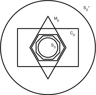
In this section we answer the question we posed in the last section. We define a Banach space of functions, to be denoted by ${{{\bm{S}}_{\negthinspace 0}}({\mathbb{R}}^{d})}$, that is very well suited for Fourier analysis, it has the tensor factorization property and consequently allows for the formulation of a kernel theorem. It therefore is the Banach space of test functions that we wish for. Figures 1 and 2 give an overview of this and the other spaces that we have considered so far. In relation to the much used Schwartz space we mention that it is a dense subspace of ${{\bm{S}}_{\negthinspace 0}}$. Functions in ${{\bm{S}}_{\negthinspace 0}}$, however, need not be differentiable.

Figure 1: An overview of some of the properties of the four Banach spaces of functions that we consider, ${\big{(}{{\bm{C}}_{\negthinspace 0}}({\mathbb{R}}^{d}),\,\|\mbox{$\,\cdot\,$}\|_{\infty}\big{)}}$, ${\big{(}{{\bm{W}}({\mathbb{R}})},\,\|\mbox{$\,\cdot\,$}\|_{\bm{W}}\big{)}}$, $({\bm{W}}_{\negthinspace\negthinspace{\operatorname{{\mathcal{F}}}}}(\mathbb{R}^{n}),\|\cdot\|_{{\bm{W}}_{\negthinspace\negthinspace{\operatorname{{\mathcal{F}}}}}})$ and $\big{(}{{{\bm{S}}_{\negthinspace 0}}({\mathbb{R}}^{d})},\|\mbox{$\,\cdot\,$}\|_{{\bm{S}}_{\negthinspace 0}}\big{)}$.

Figure 2: The figure visualizes the collection of the spaces that we have considered and their relative (non-)inclusions. In the center we have ${{\bm{S}}_{\negthinspace 0}}$. Slightly larger, the octagon, is the space ${\bm{W}}_{\negthinspace\negthinspace{\operatorname{{\mathcal{F}}}}}$. In turn, it is contained in Wiener’s algebra ${\bm{W}}$, which is depicted by a hexagon. The space ${{\bm{C}}_{\negthinspace 0}}$ contains all these three spaces, but it is not completely contained in ${{\bm{M}}_{\negthinspace b}}$. The space ${{\bm{S}}_{\negthinspace 0}^{\prime}}$ contains all spaces. The spaces ${{{\bm{S}}_{\negthinspace 0}}({\mathbb{R}}^{d})}$, ${{\bm{W}}_{\negthinspace\negthinspace{\operatorname{{\mathcal{F}}}}}\!\,({{{\mathbb{R}}^{d}}})}$ and ${{\bm{S}}_{\negthinspace 0}^{\prime}}$ are invariant under the Fourier transform. This is represented by a symbol that does not change under rotation by 90 degrees.

First we have to introduce the Short-Time Fourier Transform (or STFT) of a function with respect to a window function $g$. There are various different assumptions which ensure the pointwise existence (and continuity) of the STFT as a function over the time-frequency plane or phase space. We introduct it as follows.

For a function $g\in{{\bm{W}}({{{\mathbb{R}}^{d}}})}$, the so-called Gabor window, which is typically a non-negative, even function concentrated near zero, we define the short-time Fourier transform with respect to $g$ of a function $f\in{{{\bm{C}}_{\negthinspace b}}({{{\mathbb{R}}^{d}}})}$ to be the function

$$\mathcal{V}_{g}:{{{\bm{C}}_{\negthinspace b}}({{{\mathbb{R}}^{d}}})}\to{{\bm{C}}_{\negthinspace b}}({{\mathbb{R}}^{2d}}),$$

$$\mathcal{V}_{g}{f}(x,\omega)=\int_{{{{\mathbb{R}}^{d}}}}f(t)\,\overline{g(t-x)}\,e^{-2\pi i\omega\,t}\,dt={\operatorname{{\mathcal{F}}}}(f\cdot\overline{T_{x}g})(\omega),\ \ x,\omega\in{{{{\mathbb{R}}^{d}}}}.$$

It is easy to see that the definition makes sense for $g\in{{\bm{W}}({{{\mathbb{R}}^{d}}})},\,f\in{{{\bm{C}}_{\negthinspace b}}({{{\mathbb{R}}^{d}}})}$ (still using the Riemann integral). Fix $g_{0}(t)=e^{-\pi\,t\cdot t}$, $t\in{{{\mathbb{R}}^{d}}}$ to be the Gaussian.

Definition 7.1.

The space ${{\bm{S}}_{\negthinspace 0}}({{{\mathbb{R}}^{d}}})$ consists of all functions $f\in{{{\bm{C}}_{\negthinspace b}}({{{\mathbb{R}}^{d}}})}$ for which $\mathcal{V}_{g_{0}}f$ is a function in ${\bm{W}}({{{\mathbb{R}}}^{2d}})$. It is endowed with the norm

$$\|\cdot\|_{{{\bm{S}}_{\negthinspace 0}}}:{{\bm{S}}_{\negthinspace 0}}({{{\mathbb{R}}^{d}}})\to\mathbb{R}^{+}_{0},\ \|f\|_{{{\bm{S}}_{\negthinspace 0}}}=\int_{{{{\mathbb{R}}}^{2d}}}\big{|}\big{(}\mathcal{V}_{g_{0}}f\big{)}(x,\omega)\big{|}\,d(x,\omega)=\|\mathcal{V}_{g_{0}}f\|_{1}.$$

Observe that this norm is well-defined, as functions in the Wiener algebra are integrable (see Section 4).

Our goal is to establish the following key result:

Theorem 7.2.

The space $\big{(}{{{\bm{S}}_{\negthinspace 0}}({\mathbb{R}}^{d})},\|\mbox{$\,\cdot\,$}\|_{{\bm{S}}_{\negthinspace 0}}\big{)}$ is a Banach space, which is isometrically invariant under the Fourier transform and time-frequency shifts, and in fact a Banach algebra under convolution as well as multiplication.

We start by observing that ${{{\bm{S}}_{\negthinspace 0}}({\mathbb{R}}^{d})}$ is a subspace of Wiener’s algebra.

Lemma 7.3.

1. The Feichtinger algebra ${{{\bm{S}}_{\negthinspace 0}}({\mathbb{R}}^{d})}$ is a subspace of and continuously embedded into the Wiener algebra ${{\bm{W}}({{{\mathbb{R}}^{d}}})}$.

2. For any $f\in{{\bm{S}}_{\negthinspace 0}}({{{\mathbb{R}}^{d}}})$ it holds that $\|f\|_{1}\leq\|f\|_{{{\bm{S}}_{\negthinspace 0}}}$ and $\|f\|_{\infty}\leq\|f\|_{{{\bm{S}}_{\negthinspace 0}}}$.

3. The mapping ${{{\bm{S}}_{\negthinspace 0}}({\mathbb{R}}^{d})}\to\mathbb{R}_{0}^{+},\ f\mapsto\|\mathcal{V}_{g_{0}}f\|_{{\bm{W}}({{{\mathbb{R}}}^{2d}})}$ is an equivalent norm on ${{{\bm{S}}_{\negthinspace 0}}({\mathbb{R}}^{d})}$.

Proof.

Observe that for any $x,s\in{{{\mathbb{R}}^{d}}}$ we have

$$|f(x)\,g_{0}(s)|\leq\|f\cdot T_{s-x}g_{0}\|_{\infty}.$$

Since $f\in{{{\bm{C}}_{\negthinspace b}}({{{\mathbb{R}}^{d}}})}$, $g_{0}\in{{\bm{W}}({{{\mathbb{R}}^{d}}})}$ and because the translation operator is continuous on ${{\bm{W}}({{{\mathbb{R}}^{d}}})}$, it follows from Lemma 4.2 that $f\cdot T_{s-x}g_{0}\in{{\bm{W}}({{{\mathbb{R}}^{d}}})}$ for any $x,s\in{{{\mathbb{R}}^{d}}}$. Furthermore, by assumption $f$ is such that

$$(x,\omega)\mapsto\mathcal{V}_{g_{0}}f(x,\omega)=\int_{{\mathbb{R}}^{d}}f(t)\,g_{0}(t-x)\,e^{-2\pi ix\cdot t}\,dt=\mathcal{F}(f\cdot T_{x}g_{0})(\omega)$$

is a function in ${\bm{W}}(\mathbb{R}^{2d})$. This implies, by Lemma 4.12, that for fixed $x\in{{{\mathbb{R}}^{d}}}$ the function $\omega\mapsto\mathcal{F}(f\cdot T_{x}g_{0})(\omega)$ belongs to ${{\bm{W}}({{{\mathbb{R}}^{d}}})}$ as well. We may therefore apply the Fourier inversion formula, so that, for any $x,s\in{{{\mathbb{R}}^{d}}}$,

$$\operatorname{\mathcal{F}}^{-1}{\operatorname{{\mathcal{F}}}}(f\cdot T_{s-x}g_{0})=f\cdot T_{s-x}g_{0}.$$

By the Riemann-Lebesgue lemma

$$\|\operatorname{\mathcal{F}}^{-1}{\operatorname{{\mathcal{F}}}}(f\cdot T_{s-x}g_{0})\|_{\infty}\leq\|{\operatorname{{\mathcal{F}}}}(f\cdot T_{s-x}g_{0})\|_{{\bm{W}}}=\sum_{m\in\mathbb{Z}^{d}}\|{\operatorname{{\mathcal{F}}}}(f\cdot T_{s-x}g_{0})\cdot\psi_{m}\|_{\infty}.$$ (40)

A combination of the observed facts yields the inequality

$$|f(x)\,g_{0}(s)|\leq\sum_{m\in\mathbb{Z}^{d}}\|{\operatorname{{\mathcal{F}}}}(f\cdot T_{s-x}g_{0})\cdot\psi_{m}\|_{\infty}.$$

Hence

$$\sup_{x\in{{{\mathbb{R}}^{d}}}}|f(x)\,g_{0}(s)\psi_{n}(x)|\leq\sum_{m\in\mathbb{Z}^{d}}\,\sup_{x,\omega\in{{{\mathbb{R}}^{d}}}}|{\operatorname{{\mathcal{F}}}}(f\cdot T_{s-x}g_{0})(\omega)\cdot\psi_{m}(\omega)\psi_{n}(x)|.$$

Summing over $n$, and using that the translation operator is continuous on ${{\bm{W}}({{{\mathbb{R}}^{d}}})}$ allows us to deduce that

$$\sum_{n\in\mathbb{Z}^{d}}\|f\cdot\psi_{n}\|_{\infty}\,|g_{0}(s)|\leq 4^{d}\,\sum_{n,m\in\mathbb{Z}^{d}}\big{|}\mathcal{V}_{g_{0}}f(x,\omega)\,\psi_{n}(x)\,\psi_{m}(\omega)\big{|}=4^{d}\|\mathcal{V}_{g_{0}}f\|_{{\bm{W}}},$$

for any $s\in{{{\mathbb{R}}^{d}}}$ and $f\in{{{\bm{S}}_{\negthinspace 0}}({\mathbb{R}}^{d})}$. It follows that

$$\|f\|_{{\bm{W}}}\leq 4^{d}\,\|g_{0}\|_{\infty}^{-1}\,\|\mathcal{V}_{g_{0}}f\|_{{\bm{W}}}=4^{d}\,\|\mathcal{V}_{g_{0}}f\|_{{\bm{W}}}.$$ (41)

We now show that there exists a constant $c>0$ such that

$$\|\mathcal{V}_{g_{0}}f\|_{{\bm{W}}}\leq c\,\|f\|_{{{\bm{S}}_{\negthinspace 0}}}\ \ \text{for all}\ \ f\in{{\bm{S}}_{\negthinspace 0}}({{{\mathbb{R}}^{d}}}).$$

We first establish the following equality: for any $f\in{{{\bm{S}}_{\negthinspace 0}}({\mathbb{R}}^{d})}$ and $x,\omega\in{{{\mathbb{R}}^{d}}}$

$$\int_{{{{\mathbb{R}}}^{2d}}}\mathcal{V}_{g_{0}}f(t,\xi)\,\overline{\mathcal{V}_{g_{0}}[E_{\omega}T_{x}g_{0}](t,\xi)}\,d(t,\xi)$$

$$=\int_{{{{\mathbb{R}}}^{2d}}}{\operatorname{{\mathcal{F}}}}(f\cdot T_{t}g_{0})(\xi)\,\overline{{\operatorname{{\mathcal{F}}}}([E_{\omega}T_{x}g_{0}]\cdot T_{t}g_{0})(\xi)}\,d(t,\xi)$$

$$\stackrel{{\scriptstyle\eqref{eq:parseval}}}{{=}}\int_{{{{\mathbb{R}}}^{2d}}}(f\cdot T_{t}g_{0})(s)\,\overline{([E_{\omega}T_{x}g_{0}]\cdot T_{t}g_{0})(s)}\,d(t,s)$$

$$=\int_{{\mathbb{R}}^{d}}f(s)\,\overline{E_{\omega}T_{x}g_{0}(s)}\,\int_{{\mathbb{R}}^{d}}g_{0}(s-t)\,g_{0}(s-t)\,dt\,ds=2^{-d/2}\,\mathcal{V}_{g_{0}}f(x,\omega).$$ (42)

The use of (30) is justified as both $f\cdot T_{t}g_{0}$ and ${\operatorname{{\mathcal{F}}}}(f\cdot T_{t}g_{0})$ are functions in the Wiener algebra (as already establish earlier in the proof). We now observe the following:

$$\|\mathcal{V}_{g_{0}}f\|_{{\bm{W}}}=\sum_{m,n\in\mathbb{Z}^{d}}\sup_{x,\omega}\big{|}\mathcal{V}_{g_{0}}f(x,\omega)\,\psi_{n}(x)\,\psi_{m}(x)\,\big{|}$$

$$\stackrel{{\scriptstyle\eqref{eq:STFT-biorth}}}{{=}}2^{d/2}\sum_{m,n\in\mathbb{Z}^{d}}\sup_{x,\omega}\Big{|}\int_{{{{\mathbb{R}}}^{2d}}}\mathcal{V}_{g_{0}}f(t,\xi)\,\overline{\mathcal{V}_{g_{0}}[E_{\omega}T_{x}g_{0}](t,\xi)}\,d(t,\xi)\,\psi_{n}(x)\,\psi_{m}(\omega)\,\Big{|}$$

$$\leq 2^{d/2}\int_{{{{\mathbb{R}}}^{2d}}}|\mathcal{V}_{g_{0}}f(t,\xi)\,\|T_{t,\xi}\mathcal{V}_{g_{0}}g_{0}\|_{{\bm{W}}}\,d(t,\xi)$$

$$\leq 2^{9d/2}\|\mathcal{V}_{g_{0}}g_{0}\|_{{\bm{W}}}\int_{\mathbb{R}^{2d}}|\mathcal{V}_{g_{0}}f(t,\xi)|\,d(t,\xi)=2^{9d/2}\,\|\mathcal{V}_{g_{0}}g_{0}\|_{{\bm{W}}}\,\|f\|_{{{\bm{S}}_{\negthinspace 0}}}.$$

The second equality follows by the boundedness of the translation operator on the Wiener algebra. Combining the just established inequality with (41) yields

$$\|f\|_{{\bm{W}}}\leq 2^{13d/2}\,\|\mathcal{V}_{g_{0}}g_{0}\|_{{\bm{W}}}\,\|f\|_{{{\bm{S}}_{\negthinspace 0}}}\ \ \text{for all}\ \ f\in{{{\bm{S}}_{\negthinspace 0}}({\mathbb{R}}^{d})}.$$

Furthermore, we have just established that

$$\|\mathcal{V}_{g_{0}}f\|_{{\bm{W}}}\leq 2^{9d/2}\,\|\mathcal{V}_{g_{0}}g_{0}\|_{{\bm{W}}}\,\|f\|_{{{\bm{S}}_{\negthinspace 0}}}\ \ \text{for all}\ \ f\in{{{\bm{S}}_{\negthinspace 0}}({\mathbb{R}}^{d})}.$$

The inequality $\|f\|_{{{\bm{S}}_{\negthinspace 0}}}\leq\|\mathcal{V}_{g_{0}}f\|_{{\bm{W}}}$ is clear from (14). We have thus shown (i) and (iii). In order to show (ii) we replace (40) with the inequality

$$\|\operatorname{\mathcal{F}}^{-1}{\operatorname{{\mathcal{F}}}}(f\cdot T_{s-x}g_{0})\|_{\infty}\leq\|{\operatorname{{\mathcal{F}}}}(f\cdot T_{s-x}g_{0})\|_{1},$$

and make similar steps as before. We then obtain the estimate

$$|f(x)g_{0}(s)|\leq\int_{{{{\mathbb{R}}^{d}}}}\big{|}\mathcal{V}_{g_{0}}f(s-x,\omega)\big{|}\,d\omega\ \ \text{for all}\ \ x,s\in{{{\mathbb{R}}^{d}}}.$$

An integration over $x\in{{{\mathbb{R}}^{d}}}$ and taking the supremum over $s$ yields

$$\|f\|_{1}\,\|g_{0}\|_{\infty}\leq\int_{{{{\mathbb{R}}}^{2d}}}\big{|}\mathcal{V}_{g_{0}}f(s-x,\omega)\big{|}\,d(x,\omega)=\|f\|_{{{\bm{S}}_{\negthinspace 0}}}.$$

Switching the role of $x$ and $s$ implies the inequality $\|f\|_{\infty}\leq\|f\|_{{{\bm{S}}_{\negthinspace 0}}}$. This shows (ii). ∎

As every function in ${{{\bm{S}}_{\negthinspace 0}}({\mathbb{R}}^{d})}$ belongs to ${{\bm{W}}({{{\mathbb{R}}^{d}}})}$ we can apply the Fourier transform to the space ${{{\bm{S}}_{\negthinspace 0}}({\mathbb{R}}^{d})}$. It turns out that ${{{\bm{S}}_{\negthinspace 0}}({\mathbb{R}}^{d})}$ is invariant under the Fourier transform.

Proposition 7.4.

The Fourier transform is an isometric bijection from ${{\bm{S}}_{\negthinspace 0}}({{{{\mathbb{R}}^{d}}}})$ onto itself, i.e.  $\|{\operatorname{{\mathcal{F}}}}f\|_{{{\bm{S}}_{\negthinspace 0}}}=\|f\|_{{{\bm{S}}_{\negthinspace 0}}}$ for all $f\in{{{\bm{S}}_{\negthinspace 0}}({\mathbb{R}}^{d})}$.

Corollary 7.5.

${{\bm{S}}_{\negthinspace 0}}({{{\mathbb{R}}^{d}}})$ is continuously embedded into ${{\bm{W}}_{\negthinspace\negthinspace{\operatorname{{\mathcal{F}}}}}\!\,({{{\mathbb{R}}^{d}}})}$.

That ${{{\bm{S}}_{\negthinspace 0}}({\mathbb{R}}^{d})}$ is a proper subspace of ${{\bm{W}}_{\negthinspace\negthinspace{\operatorname{{\mathcal{F}}}}}\!\,({{{\mathbb{R}}^{d}}})}$ was shown by Losert [35, Theorem 2]. Observe that the inclusion ${{{\bm{S}}_{\negthinspace 0}}({\mathbb{R}}^{d})}\subset{{\bm{W}}_{\negthinspace\negthinspace{\operatorname{{\mathcal{F}}}}}\!\,({{{\mathbb{R}}^{d}}})}$ implies that all the statements in relation to the Fourier transform in Section 5 also hold for all functions in ${{{\bm{S}}_{\negthinspace 0}}({\mathbb{R}}^{d})}$.

Proof of Proposition 7.4.   First of all ${{{\bm{S}}_{\negthinspace 0}}({\mathbb{R}}^{d})}\subset{{\bm{W}}({{{\mathbb{R}}^{d}}})}$, so that ${\operatorname{{\mathcal{F}}}}f$, is a well-defined function in ${{{\bm{C}}_{\negthinspace 0}}({\mathbb{R}}^{d})}$. Since $g_{0}\in{{\bm{W}}({{{\mathbb{R}}^{d}}})}$ and ${{{\bm{S}}_{\negthinspace 0}}({\mathbb{R}}^{d})})\subset{{\bm{W}}({{{\mathbb{R}}^{d}}})}$, we can use the fundamental identity of Fourier analysis to establish the following,

$$\mathcal{V}_{g_{0}}\hat{f}(x,\omega) =\int_{{\mathbb{R}}^{d}}\hat{f}(t)\,\overline{g_{0}(t-x)}e^{-2\pi i\omega t}\,dt\stackrel{{\scriptstyle\eqref{fund-Fourier0}}}{{=}}\int_{{\mathbb{R}}^{d}}f(t)\,{\operatorname{{\mathcal{F}}}}\big{(}\overline{E_{\omega}T_{x}g_{0}}\big{)}(t)\,dt$$

$$=e^{-2\pi ix\cdot\omega}\,\mathcal{V}_{g_{0}}{f}(-\omega,x).$$

Observe that the phase factor $e^{2\pi ix\cdot\omega}$ and also the change of variable $(x,\omega)\mapsto(-\omega,x)$ are continuous operators on the Wiener algebra, so that also $\mathcal{V}_{g_{0}}\hat{f}$ belongs to ${\bm{W}}({{{\mathbb{R}}}^{2d}})$. Moreover, the operations leave the ${{\bm{S}}_{\negthinspace 0}}$-norm invariant. Indeed,

$$\|\hat{f}\|_{{{\bm{S}}_{\negthinspace 0}}}=\int_{{{{\mathbb{R}}}^{2d}}}|\mathcal{V}_{g_{0}}\hat{f}(x,\omega)|\,d(x,\omega)=\int_{{{{\mathbb{R}}}^{2d}}}|e^{-2\pi ix\cdot\omega}\,\mathcal{V}_{g_{0}}{f}(-\omega,x)|\,d(x,\omega)$$

$$=\int_{{{{\mathbb{R}}}^{2d}}}|\mathcal{V}_{g_{0}}f(x,\omega)|\,d(x,\omega)=\|f\|_{{{\bm{S}}_{\negthinspace 0}}}.$$

The same proof shows that also the inverse Fourier transform maps ${{\bm{S}}_{\negthinspace 0}}({{{\mathbb{R}}^{d}}})$ into itself. It is therefore clear that ${\operatorname{{\mathcal{F}}}}$ is a continuous bijection on ${{\bm{S}}_{\negthinspace 0}}({{{\mathbb{R}}^{d}}})$.

Concerning the continuity properties of the translation and modulation operator we easily establish the following.

Lemma 7.6.

1. Translation and modulation operators are isometries on ${{\bm{S}}_{\negthinspace 0}}({{{\mathbb{R}}^{d}}})$:

   $$\|E_{\omega}T_{x}f\|_{{{\bm{S}}_{\negthinspace 0}}}=\|f\|_{{{\bm{S}}_{\negthinspace 0}}}\ \ \text{for all}\ \ x,\omega\in{{{\mathbb{R}}^{d}}}\ \ \text{and}\ \ f\in{{\bm{S}}_{\negthinspace 0}}({{{\mathbb{R}}^{d}}}).$$ (43)

2. If $f$ belongs to ${{\bm{S}}_{\negthinspace 0}}({{{\mathbb{R}}^{d}}})$, then so does $\overline{f}$ and $f^{\checkmark}$ and

   $$\|\overline{f}\|_{{{\bm{S}}_{\negthinspace 0}}}=\|f^{\checkmark}\|_{{{\bm{S}}_{\negthinspace 0}}}=\|f\|_{{{\bm{S}}_{\negthinspace 0}}}\ \ \text{for all}\ \ f\in{{\bm{S}}_{\negthinspace 0}}({{{\mathbb{R}}^{d}}}).$$ (44)

Proof.

Observe that

$$\mathcal{V}_{g_{0}}(E_{\omega}T_{x}f)(t,s)=e^{2\pi i\,x\cdot(\omega-s)}\,\mathcal{V}_{g_{0}}f(t-x,s-\omega).$$ (45)

Since translation and the phase factor leave the Wiener algebra invariant it follows that $\mathcal{V}_{g_{0}}E_{\omega}T_{x}f\in{\bm{W}}({{{\mathbb{R}}}^{2d}})$. Hence $E_{\omega}T_{x}f\in{{\bm{S}}_{\negthinspace 0}}({{{\mathbb{R}}^{d}}})$ and moreover

$$\|E_{\omega}T_{x}f\|_{{{\bm{S}}_{\negthinspace 0}}} =\int_{{{{\mathbb{R}}}^{2d}}}|\mathcal{V}_{g_{0}}(E_{\omega}T_{x}g_{0})(t,s)|\,d(x,\omega)$$

$$=\int_{{{{\mathbb{R}}}^{2d}}}|e^{2\pi i\,x\cdot(\omega-s)}\,\mathcal{V}_{g_{0}}f(t-x,s-\omega)|\,d(t,s)$$

$$=\int_{{{{\mathbb{R}}}^{2d}}}|\mathcal{V}_{g_{0}}f(t,s)\,d(t,s)=\|f\|_{{{\bm{S}}_{\negthinspace 0}}}$$

for any pair $(x,\omega)\in{{{\mathbb{R}}}^{2d}}$. The statement in (ii) is shown in a similar fashion. ∎

Just as the Wiener algebra and ${\bm{W}}_{\negthinspace\negthinspace{\operatorname{{\mathcal{F}}}}}$, also ${{\bm{S}}_{\negthinspace 0}}$ behaves in a nice way with respect to multiplication and convolution.

Lemma 7.7.

The Banach space $\big{(}{{{\bm{S}}_{\negthinspace 0}}({\mathbb{R}}^{d})},\|\mbox{$\,\cdot\,$}\|_{{\bm{S}}_{\negthinspace 0}}\big{)}$ is a Banach algebra with respect to pointwise multiplication and convolution. Indeed, for any $f_{1},f_{2}\in{{{\bm{S}}_{\negthinspace 0}}({\mathbb{R}}^{d})}$, the functions $f_{1}\cdot f_{2}$ and $f_{1}*f_{2}$ also belong to ${{{\bm{S}}_{\negthinspace 0}}({\mathbb{R}}^{d})}$ and

$$\|f_{1}\cdot f_{2}\|_{{{\bm{S}}_{\negthinspace 0}}}\leq\|f_{1}\|_{{{\bm{S}}_{\negthinspace 0}}}\,\|f_{2}\|_{{{\bm{S}}_{\negthinspace 0}}}\ \ \text{and}\ \ \|f_{1}*f_{2}\|_{{{\bm{S}}_{\negthinspace 0}}}\leq\|f_{1}\|_{{{\bm{S}}_{\negthinspace 0}}}\,\|f_{2}\|_{{{\bm{S}}_{\negthinspace 0}}}.$$

Proof.

Let us first establish $f_{1}\cdot f_{2}$ belongs to ${{{\bm{S}}_{\negthinspace 0}}({\mathbb{R}}^{d})}$.

$$\|\mathcal{V}_{g_{0}}(f_{1}\cdot f_{2})\|_{{\bm{W}}} =\sum_{m,n\in\mathbb{Z}^{d}}\sup_{x,\omega\in{{{\mathbb{R}}^{d}}}}\big{|}{\operatorname{{\mathcal{F}}}}(f_{1}\cdot f_{2}\cdot T_{x}g_{0})(\omega)\,\psi_{n}(x)\,\psi_{m}(\omega)\,\big{|}$$

$$=\sum_{m,n\in\mathbb{Z}^{d}}\sup_{x,\omega\in{{{\mathbb{R}}^{d}}}}\big{|}{\operatorname{{\mathcal{F}}}}(f_{1})*{\operatorname{{\mathcal{F}}}}(f_{2}\cdot T_{x}g_{0})(\omega)\,\psi_{n}(x)\,\psi_{m}(\omega)\big{|}$$

$$=\sum_{m,n\in\mathbb{Z}^{d}}\sup_{x,\omega\in{{{\mathbb{R}}^{d}}}}\Big{|}\int_{{\mathbb{R}}^{d}}{\operatorname{{\mathcal{F}}}}(f_{2}\cdot T_{x}g_{0})(\omega-t)\,\hat{f}_{1}(t)\,dt\,\psi_{n}(x)\,\psi_{m}(\omega)\Big{|}$$

$$\leq\sum_{m,n\in\mathbb{Z}^{d}}\sup_{x,\omega\in{{{\mathbb{R}}^{d}}}}\int_{{\mathbb{R}}^{d}}|{\operatorname{{\mathcal{F}}}}(f_{2}\cdot T_{x}g_{0})(\omega-t)\,\psi_{m}(\omega)|\,|\hat{f}_{1}(t)|\,dt\,\psi_{n}(x)$$

$$\leq\sum_{m,n\in\mathbb{Z}^{d}}\sup_{x,\omega\in{{{\mathbb{R}}^{d}}}}\int_{{\mathbb{R}}^{d}}\sup_{\omega\in{{{\mathbb{R}}^{d}}}}|{\operatorname{{\mathcal{F}}}}(f_{2}\cdot T_{x}g_{0})(\omega)\,\psi_{m}(\omega+t)|\,|\hat{f}_{1}(t)|\,dt\,\psi_{n}(x)$$

$$\leq 4^{d}\sum_{m,n\in\mathbb{Z}^{d}}\sup_{x\in{{{\mathbb{R}}^{d}}}}\int_{{\mathbb{R}}^{d}}\sup_{\omega\in{{{\mathbb{R}}^{d}}}}|{\operatorname{{\mathcal{F}}}}(f_{2}\cdot T_{x}g_{0})(\omega)\,\psi_{m}(\omega)|\,|\hat{f}_{1}(t)|\,dt\,\psi_{n}(x)$$

$$\leq 4^{d}\|\hat{f}_{1}\|_{{\bm{W}}}\,\|f_{2}\|_{{{\bm{S}}_{\negthinspace 0}}}\leq 16^{d}\,\|f_{1}\|_{{{\bm{S}}_{\negthinspace 0}}}\,\|f_{2}\|_{{{\bm{S}}_{\negthinspace 0}}}<\infty.$$

In the third inequality we used the same method as in the proof of Lemma 4.3 to get rid of the translation by $x$. The inequality for the convolution follows by the just established inequality, the equality ${\operatorname{{\mathcal{F}}}}(f_{1}\cdot f_{2})=\hat{f}_{1}*\hat{f}_{2}$ and the fact that the Fourier transform is a bijection on ${{\bm{S}}_{\negthinspace 0}}$. We have thus established that $\mathcal{V}_{g_{0}}(f_{1}\cdot f_{2})\in{\bm{W}}({{{\mathbb{R}}}^{2d}})$ and $\mathcal{V}_{g_{0}}(f_{1}*f_{2})\in{\bm{W}}({{{\mathbb{R}}}^{2d}})$, i.e., the convolution and pointwise product of $f_{1},f_{2}$ belong to ${{\bm{S}}_{\negthinspace 0}}$ again. Concerning the desired estimates, we find that

$$\|f_{1}*f_{2}\|_{{{\bm{S}}_{\negthinspace 0}}} =\int_{{{{\mathbb{R}}^{d}}}}\int_{{{{\mathbb{R}}^{d}}}}\big{|}{\operatorname{{\mathcal{F}}}}([f_{1}*f_{2}]\cdot T_{x}g_{0})(\omega)\big{|}\,dx\,d\omega$$

$$=\int_{{\mathbb{R}}^{d}}\int_{{\mathbb{R}}^{d}}\big{|}\big{(}f_{1}*f_{2}*E_{\omega}g_{0}\big{)}(x)\big{|}\,dx\,d\omega$$

$$\leq\|f_{1}\|_{1}\,\int_{{\mathbb{R}}^{d}}\int_{{\mathbb{R}}^{d}}|\big{(}f_{2}*E_{\omega}g_{0}\big{)}(x)\,dx\,d\omega$$

$$=\|f_{1}\|_{1}\,\|f_{2}\|_{{{\bm{S}}_{\negthinspace 0}}}\leq\|f_{1}\|_{{{\bm{S}}_{\negthinspace 0}}}\,\|f_{2}\|_{{{\bm{S}}_{\negthinspace 0}}}.$$

The first inequality is an application of (18). The second inequality follows by Lemma 7.3(ii). The inequality for the pointwise product follows by properties of the Fourier transform as mentioned before.∎

Among other useful properties of ${{{\bm{S}}_{\negthinspace 0}}({\mathbb{R}}^{d})}$ are the following ones. In particular, ${{\bm{S}}_{\negthinspace 0}}$ has the tensor factorization property.

Theorem 7.8.

1. For any invertible $d\times d$-matrix $A$ the operator

   $$\alpha_{A}:{{{\bm{S}}_{\negthinspace 0}}({\mathbb{R}}^{d})}\to{{{\bm{S}}_{\negthinspace 0}}({\mathbb{R}}^{d})},\ \alpha_{A}f(x)=|\det(A)|^{1/2}\,f(Ax),\ \ x\in{{{\mathbb{R}}^{d}}},$$

   is a continuous bijection on ${{{\bm{S}}_{\negthinspace 0}}({\mathbb{R}}^{d})}$.

2. For any $m\in\mathbb{N}$ such that $0<m<d$, the operator

   $$\mathcal{R}_{m}:{{{\bm{S}}_{\negthinspace 0}}({\mathbb{R}}^{d})}\to{{\bm{S}}_{\negthinspace 0}}(\mathbb{R}^{m}),\ \mathcal{R}_{m}f(x^{(1)},\ldots,x^{(m)})=f(x^{(1)},\ldots,x^{(m)},0,\ldots,0),\ x^{(i)}\in\mathbb{R},$$

   is a continuous surjection.

3. The sampling of a function on ${{{{\mathbb{R}}^{d}}}}$ at the integer-lattice points $\mathbb{Z}^{d}$

   $$\mathcal{R}_{\mathbb{Z}^{d}}:{{{\bm{S}}_{\negthinspace 0}}({\mathbb{R}}^{d})}\to\ell^{1}(\mathbb{Z}^{d}),\ \mathcal{R}_{\mathbb{Z}^{d}}f(k)=f(k),\ \ k\in\mathbb{Z}^{d}$$

   is a continuous and surjective operator from ${{\bm{S}}_{\negthinspace 0}}({{{\mathbb{R}}^{d}}})$ onto $\ell^{1}(\mathbb{Z}^{d})$.

4. For any $m\in\mathbb{N}$ such that $0<m<d$ the operator

   $$\mathcal{P}_{m}:{{\bm{S}}_{\negthinspace 0}}({{{{\mathbb{R}}^{d}}}})\to{{\bm{S}}_{\negthinspace 0}}({\mathbb{R}}^{m}),$$

   $$\mathcal{P}_{m}f(x)=\int_{\mathbb{R}^{n-m}}f(x^{(1)},\ldots,x^{(m)},x^{(m+1)},\ldots,x^{(n)})\,dx^{(m+1)}\ldots dx^{(n)},$$

   $$x=(x^{(1)},\ldots,x^{(m)})\in{{{\mathbb{R}}}^{m}}.$$

   is a continuous surjection.

5. The periodization of functions on ${{{{\mathbb{R}}^{d}}}}$ with respect to the integer lattice $\mathbb{Z}^{n}$

   $$\mathcal{P}_{\mathbb{Z}^{n}}:{{\bm{S}}_{\negthinspace 0}}({{{{\mathbb{R}}^{d}}}})\to{\bm{A}}([0,1]^{n}),\ \mathcal{P}f(x)=\sum_{k\in\mathbb{Z}^{n}}f(x+k),\ \ x\in[0,1]^{n},$$

   is a continuous and surjective operator from ${{{\bm{S}}_{\negthinspace 0}}({\mathbb{R}}^{d})}$ onto $A([0,1]^{n})$, the space of all $\mathbb{Z}^{n}$-periodic functions with absolutely-summable Fourier coefficients.

6. ${{\bm{S}}_{\negthinspace 0}}({\mathbb{R}^{n}})\,\widehat{\otimes}\,{{\bm{S}}_{\negthinspace 0}}({\mathbb{R}^{m}})={{\bm{S}}_{\negthinspace 0}}(\mathbb{R}^{n+m})$ for any $n,m\in\mathbb{N}$.

Proof.

We are not in the position to give a proof, as this requires more theory and details about ${{\bm{S}}_{\negthinspace 0}}$ than we are willing to give here. The statements all follow from [14, Theorem 7]. ∎

To highlight the role of ${{\bm{S}}_{\negthinspace 0}}({{{\mathbb{R}}^{d}}})$ among all Banach spaces of functions within ${{\bm{W}}({{{\mathbb{R}}^{d}}})}$, we give the following characterization. It is a direct consequence of [32, Theorem 7.6]

Theorem 7.9.

For each $d\in\mathbb{N}$ let $({\bm{B}}({{{\mathbb{R}}^{d}}}),\|\cdot\|_{{\bm{B}}})$ be a non-trivial Banach space such that ${\bm{B}}({\mathbb{R}^{d}})\subseteq{\bm{W}}({\mathbb{R}^{d}})$. If for each $d\in\mathbb{N}$ the Banach space ${\bm{B}}({\mathbb{R}^{d}})$ has the properties that

1. there is a constant $c>0$ such that $\|f\|_{{\bm{W}}({{{\mathbb{R}}^{d}}})}\leq c\,\|f\|_{{\bm{B}}({{{\mathbb{R}}^{d}}})}$ for all $f\in{\bm{B}}({{{\mathbb{R}}^{d}}})$,

2. for all $(x,\omega)\in{{{\mathbb{R}}}^{2d}}$ the time-frequency shift operators $E_{\omega}T_{x}$ is bounded on ${\bm{B}}({{{\mathbb{R}}^{d}}})$ with a uniformly bounded operator norm over all $(x,\omega)\in{{{\mathbb{R}}}^{2d}}$,

3. for every invertible $d\times d$-matrix $A$ the operator $f\mapsto f\circ A$ is bounded on ${\bm{B}}({{{\mathbb{R}}^{d}}})$,

4. the Fourier transform is a bounded operator from ${\bm{B}}({{{\mathbb{R}}^{d}}})$ into ${\bm{W}}({{{\mathbb{R}}^{d}}})$,

5. and ${\bm{B}}({\mathbb{R}^{n}})\,\widehat{\otimes}\,{\bm{B}}({\mathbb{R}^{m}})={\bm{B}}(\mathbb{R}^{n+m})$ for all $n,m\in\mathbb{N}$,

then $({\bm{B}}({{{{\mathbb{R}}^{d}}}}),\|\cdot\|_{{\bm{B}}})=\big{(}{{{\bm{S}}_{\negthinspace 0}}({\mathbb{R}}^{d})},\|\mbox{$\,\cdot\,$}\|_{{\bm{S}}_{\negthinspace 0}}\big{)}$ for all $d\in\mathbb{N}$.

8 The shortcut to distribution theory

In the previous sections we described several Banach spaces of continuous functions on ${{{\mathbb{R}}^{d}}}$ that have useful properties. Figure 1 gives a brief overview. Based on this, we recognize ${{\bm{S}}_{\negthinspace 0}}$ as a useful space of test-functions. It has all the properties that we wish for. We will consider its dual space $({{{\bm{S}}_{\negthinspace 0}^{\prime}}({\mathbb{R}}^{d})},\|\mbox{$\,\cdot\,$}\|_{{{\bm{S}}_{\negthinspace 0}^{\prime}}})$ as a suitably large reservoir of “everything else” that is worth to investigate. We call elements in ${{\bm{S}}_{\negthinspace 0}^{\prime}}$ for distributions.

The shortcut to distribution theory is here the fact that we have established a useful Banach space as our space of test functions. Hence we do not require the more technical details that are typically needed to properly understand the Fréchet space formed by the Schwartz functions. Similarly, the dual space, here the Banach space ${{{\bm{S}}_{\negthinspace 0}^{\prime}}({\mathbb{R}}^{d})}$ is also much more convenient that the space of tempered distributions (the dual of the Schwartz space). Ergo, with less mathematical effort we can describe and achieve much of the same type of results that the Schwartz space and the temperate distributions are typically used for.

One of the most important concepts of the dual space is that it is possible to extend operators that act on ${{\bm{S}}_{\negthinspace 0}}$ to operators that act on ${{\bm{S}}_{\negthinspace 0}^{\prime}}$. In particular, the properties of ${{\bm{S}}_{\negthinspace 0}}$ allow us to define the Fourier transform of elements in ${{\bm{S}}_{\negthinspace 0}^{\prime}}$ (this is also possible to do with ${\bm{W}}_{\negthinspace\negthinspace{\operatorname{{\mathcal{F}}}}}$ and ${\bm{W}}_{\negthinspace\negthinspace{\operatorname{{\mathcal{F}}}}}^{\prime}$). Before we get to this, we need to introduce ${{\bm{S}}_{\negthinspace 0}^{\prime}}$ properly.

The dual space ${{{\bm{S}}_{\negthinspace 0}^{\prime}}({\mathbb{R}}^{d})}$, consists of bounded, linear functionals $\sigma:{{{\bm{S}}_{\negthinspace 0}}({\mathbb{R}}^{d})}\to\mathbb{C}$. It is a Banach space with respect to the usual functional norm

$$\|\sigma\|_{{{\bm{S}}_{\negthinspace 0}^{\prime}}}=\sup_{{f\in{{{\bm{S}}_{\negthinspace 0}}({\mathbb{R}}^{d})},\,\,\|f\|_{{{\bm{S}}_{\negthinspace 0}}}=1}}|\sigma(f)|.$$ (46)

This topology is often too strong. Another weaker, yet at least as natural topology on ${{\bm{S}}_{\negthinspace 0}^{\prime}}$ is the topology it inherits from ${{\bm{S}}_{\negthinspace 0}}$: we say that a sequence $(\sigma_{n})$ in ${{{\bm{S}}_{\negthinspace 0}^{\prime}}({\mathbb{R}}^{d})}$ converges in the weak^∗topology towards $\sigma_{0}\in{{{\bm{S}}_{\negthinspace 0}^{\prime}}({\mathbb{R}}^{d})}$ exactly if

$$\lim_{n}\big{|}\big{(}\sigma_{n}-\sigma_{0}\big{)}(f)\big{|}=0\ \ \text{for all}\ \ f\in{{\bm{S}}_{\negthinspace 0}}({{{\mathbb{R}}^{d}}}).$$ (47)

Now every $h\in{{{\bm{C}}_{\negthinspace b}}({{{\mathbb{R}}^{d}}})}$ (and many more) defines a distribution $\sigma_{h}\in{{{\bm{S}}_{\negthinspace 0}^{\prime}}({\mathbb{R}}^{d})}$ via the injective embedding operator

$$\iota:{{{\bm{C}}_{\negthinspace b}}({{{\mathbb{R}}^{d}}})}\to{{{\bm{S}}_{\negthinspace 0}^{\prime}}({\mathbb{R}}^{d})},\ \iota(k)=\sigma_{h}=f\mapsto\int_{{\mathbb{R}}^{d}}f(t)\,h(t)\,dt.$$ (48)

Also, any $\mu\in{{\bm{M}}_{\negthinspace b}}({{{{\mathbb{R}}^{d}}}})$ defines a distribution $\sigma_{\mu}\in{{{\bm{S}}_{\negthinspace 0}^{\prime}}({\mathbb{R}}^{d})}$ by the rule

$$\sigma_{\mu}(f)=\mu(f)\ \ \text{for all}\ \ f\in{{\bm{S}}_{\negthinspace 0}}({{{\mathbb{R}}^{d}}}).$$

The mapping $\mu\mapsto\sigma_{\mu}$ provides a continuous embedding ${{\bm{M}}_{\negthinspace b}}({{{\mathbb{R}}^{d}}})$ into ${{{\bm{S}}_{\negthinspace 0}^{\prime}}({\mathbb{R}}^{d})}$.

Definition 8.1.

Assume $T$ is a continuous operator from ${{{\bm{S}}_{\negthinspace 0}}({\mathbb{R}}^{d})}$ into ${{{\bm{S}}_{\negthinspace 0}}({\mathbb{R}}^{d})}$. We say that the operator $\widetilde{T}:{{{\bm{S}}_{\negthinspace 0}^{\prime}}({\mathbb{R}}^{d})}\to{{{\bm{S}}_{\negthinspace 0}^{\prime}}({\mathbb{R}}^{d})}$ is an extension of $T$ if the following holds,

1. $\widetilde{T}$ is weak^∗-weak^∗ continuous,

2. $\widetilde{T}\circ\iota(k)=\iota\circ T(k)$ (or, equivalently, $\widetilde{T}\sigma_{k}=\sigma_{\,Tk}$ ) for all $k\in{{{\bm{S}}_{\negthinspace 0}}({\mathbb{R}}^{d})}$.

Lemma 8.2.

The Fourier transform ${\operatorname{{\mathcal{F}}}}$, translation operator $T_{x}$, $x\in{{{\mathbb{R}}^{d}}}$, modulation operator $E_{\omega}$, $\omega\in{{{\mathbb{R}}^{d}}}$, and the coordinate transform $\alpha_{A}$, $A\in\textnormal{GL}_{d}(\mathbb{R})$ are extended from operators on ${{{\bm{S}}_{\negthinspace 0}}({\mathbb{R}}^{d})}$ to operators on ${{\bm{S}}_{\negthinspace 0}^{\prime}}({{{\mathbb{R}}^{d}}})$ in the following way: for any $f\in{{\bm{S}}_{\negthinspace 0}}({{{\mathbb{R}}^{d}}})$ and $\sigma\in{{\bm{S}}_{\negthinspace 0}^{\prime}}({{{\mathbb{R}}^{d}}})$

$$\widetilde{{\operatorname{{\mathcal{F}}}}} :{{{\bm{S}}_{\negthinspace 0}^{\prime}}({\mathbb{R}}^{d})}\to{{{\bm{S}}_{\negthinspace 0}^{\prime}}({\mathbb{R}}^{d})},\ \big{(}\widetilde{{\operatorname{{\mathcal{F}}}}}\sigma\big{)}(f)=\sigma({\operatorname{{\mathcal{F}}}}f),$$

$$\widetilde{T}_{x} :{{{\bm{S}}_{\negthinspace 0}^{\prime}}({\mathbb{R}}^{d})}\to{{{\bm{S}}_{\negthinspace 0}^{\prime}}({\mathbb{R}}^{d})},\ \big{(}\widetilde{T}_{x}\sigma\big{)}(f)=\sigma(T_{-x}f),$$

$$\widetilde{E}_{\omega} :{{{\bm{S}}_{\negthinspace 0}^{\prime}}({\mathbb{R}}^{d})}\to{{{\bm{S}}_{\negthinspace 0}^{\prime}}({\mathbb{R}}^{d})},\ \big{(}\widetilde{E}_{\omega}\sigma\big{)}(f)=\sigma(E_{\omega}f),$$

$$\widetilde{\alpha}_{A} :{{{\bm{S}}_{\negthinspace 0}^{\prime}}({\mathbb{R}}^{d})}\to{{{\bm{S}}_{\negthinspace 0}^{\prime}}({\mathbb{R}}^{d})},\ \big{(}\widetilde{\alpha}_{A}\sigma\big{)}(f)=\sigma(\alpha_{A^{-1}}f).$$

Proof.

We only show the result for the Fourier transform. The statements for the other operators are proven in the same fashion. We have to show that $\widetilde{F}$ satisfies Definition 8.1. In order to show the weak^∗-weak^∗continuity, let $(\sigma_{n})$ be a sequence in ${{{\bm{S}}_{\negthinspace 0}^{\prime}}({\mathbb{R}}^{d})}$ that converges in the weak^∗-sense towards $\sigma_{0}$. We have to show that then also $\widetilde{{\operatorname{{\mathcal{F}}}}}\sigma_{n}\xrightarrow{\text{w}^{*}}\widetilde{{\operatorname{{\mathcal{F}}}}}\sigma_{0}$. This follows easily from the definition of $\widetilde{{\operatorname{{\mathcal{F}}}}}$,

$$\lim_{n}\big{|}\big{(}\widetilde{{\operatorname{{\mathcal{F}}}}}\sigma_{n}-\widetilde{{\operatorname{{\mathcal{F}}}}}\sigma_{0}\big{)}(f)\big{|}=\lim_{n}\big{|}\big{(}\widetilde{{\operatorname{{\mathcal{F}}}}}(\sigma_{n}-\sigma_{0})\big{)}(f)\big{|}$$

$$=\lim_{n}\big{|}\big{(}\sigma_{n}-\sigma_{0}\big{)}({\operatorname{{\mathcal{F}}}}f)\big{|}=0,$$

where the last equality follows by assumption. It remains to show that Definition 8.1(ii) is satisfied. We observe that for all $f,k\in{{{\bm{S}}_{\negthinspace 0}}({\mathbb{R}}^{d})}$

$$\big{(}\widetilde{{\operatorname{{\mathcal{F}}}}}\circ\iota(k)\big{)}(f)=\big{(}\iota(k)\big{)}({\operatorname{{\mathcal{F}}}}f)=\int_{{\mathbb{R}}^{d}}\hat{f}(t)\,k(t)\,dt$$

$$\big{(}\iota\circ{\operatorname{{\mathcal{F}}}}(k)\big{)}(f)=\int_{{\mathbb{R}}^{d}}f(t)\,\hat{k}(t)\,dt.$$

It follows from (25) that the latter two integrals are the same, so that $\widetilde{{\operatorname{{\mathcal{F}}}}}\circ\iota(k)=\iota\circ{\operatorname{{\mathcal{F}}}}(k)$, as desired. ∎

Consider the Dirac delta,

$$\delta_{x}:{{{\bm{S}}_{\negthinspace 0}}({\mathbb{R}}^{d})}\to\mathbb{C},\quad\delta_{x}(f)=f(x),\ x\in{{{\mathbb{R}}^{d}}},$$

It is easy to show that $\widehat{\delta_{x}}=\widetilde{{\operatorname{{\mathcal{F}}}}}\delta_{x}$ is the distribution given by

$$\widetilde{{\operatorname{{\mathcal{F}}}}}\delta_{x}:{{\bm{S}}_{\negthinspace 0}}({{{\mathbb{R}}^{d}}})\to\mathbb{C},\quad\widetilde{{\operatorname{{\mathcal{F}}}}}\delta_{x}(f)=\hat{f}(x)=\int_{{\mathbb{R}}^{d}}f(t)\,e^{-2\pi ix\cdot t}\,dt.$$

Or, equivalently, $\widetilde{{\operatorname{{\mathcal{F}}}}}\delta_{x}=\iota({e_{x}})$, where $e_{x}\in{{{\bm{C}}_{\negthinspace b}}({{{\mathbb{R}}^{d}}})}$ is given by $e_{x}(t)=e^{-2\pi ix\cdot t}$. This can be formulated as to say that “the Fourier transform of the Dirac delta distribution at $x$, $\delta_{x}$, is the function $e_{x}(t)=e^{-2\pi it\cdot x}$”. Or, equivalently, “the Fourier transform of the function $e_{x}(t)=e^{2\pi it\cdot x}$, $t\in{{{\mathbb{R}}^{d}}}$, is the Dirac delta distribution at $x$, $\delta_{x}$”.

Remark 8.3.

This is the characteristic property of the Fourier transform: it maps pure frequencies into Dirac measures and vice versa (see [37], (4.36)).

Consider now the Dirac comb or Shah distribution for a given invertible $d\times d$ matrix $A$, it is the element of ${{{\bm{S}}_{\negthinspace 0}^{\prime}}({\mathbb{R}}^{d})}$ defined by

$${\makebox[9.90276pt][s]{$\sqcup$\hfill$\sqcup$}\,\,}_{A}:{{{\bm{S}}_{\negthinspace 0}}({\mathbb{R}}^{d})}\to\mathbb{C},\ {\makebox[9.90276pt][s]{$\sqcup$\hfill$\sqcup$}\,\,}_{A}(f)=\sum_{k\in\mathbb{Z}^{d}}f(Ak).$$

By definition of $\widetilde{{\operatorname{{\mathcal{F}}}}}$ and a use of the Poisson summation formula (34), one gets

$$\widetilde{{\operatorname{{\mathcal{F}}}}}({\makebox[9.90276pt][s]{$\sqcup$\hfill$\sqcup$}\,\,}_{A})=|\det(A)|^{-1}\,{\makebox[9.90276pt][s]{$\sqcup$\hfill$\sqcup$}\,\,}_{A^{\dagger}}.$$

We define multiplication and convolution of a distribution $\sigma\in{{{\bm{S}}_{\negthinspace 0}^{\prime}}({\mathbb{R}}^{d})}$ with a test function $g\in{{{\bm{S}}_{\negthinspace 0}}({\mathbb{R}}^{d})}$ to be the distribution $\sigma\in{{{\bm{S}}_{\negthinspace 0}^{\prime}}({\mathbb{R}}^{d})}$ defined as follows:

Definition 8.4.

$$\big{(}\sigma*g\big{)}(f)=\sigma(g^{\checkmark}\!*f)\ \ \text{and}\ \ \big{(}\sigma\cdot g\big{)}(f)=\sigma(g\cdot f)\ \ \quad\ f\in{{{\bm{S}}_{\negthinspace 0}}({\mathbb{R}}^{d})}.$$

The definition of the convolution is consistent with the definition

$$(\sigma*g)(t)=\sigma(T_{t}g^{\checkmark}),\ \ t\in{{{\mathbb{R}}^{d}}}.$$

Consequently we have ${{{\bm{S}}_{\negthinspace 0}}({\mathbb{R}}^{d})}\ast{{{\bm{S}}_{\negthinspace 0}^{\prime}}({\mathbb{R}}^{d})}\subset{{{\bm{C}}_{\negthinspace b}}({{{\mathbb{R}}^{d}}})}$, viewed as a subspace of ${{{\bm{S}}_{\negthinspace 0}^{\prime}}({\mathbb{R}}^{d})}$. Observe that ${\makebox[9.90276pt][s]{$\sqcup$\hfill$\sqcup$}\,\,}_{A}*g$ equals the $A$-period function in ${{{\bm{C}}_{\negthinspace b}}({{{\mathbb{R}}^{d}}})}$ given by

$$\big{(}{\makebox[9.90276pt][s]{$\sqcup$\hfill$\sqcup$}\,\,}_{A}*g\big{)}(t)=\sum_{k\in\mathbb{Z}^{d}}g(t+Ak),\ \ t\in{{{\mathbb{R}}^{d}}},$$

where the convergence of the series is uniform and absolute within ${\big{(}{{\bm{C}}_{\negthinspace b}}({\mathbb{R}}^{d}),\,\|\mbox{$\,\cdot\,$}\|_{\infty}\big{)}}$. Furthermore, one can show that

$$\widetilde{{\operatorname{{\mathcal{F}}}}}(\sigma*g)=(\widetilde{{\operatorname{{\mathcal{F}}}}}\sigma)\cdot({{\operatorname{{\mathcal{F}}}}}g),\ \ \widetilde{{\operatorname{{\mathcal{F}}}}}(\sigma\cdot g)=\widetilde{{\operatorname{{\mathcal{F}}}}}\sigma*{{\operatorname{{\mathcal{F}}}}}g.$$ (49)

We shall use these relations in Section 10, where we take a look at the Shannon sampling theorem.

Proof of (49). This follows by the definition of the extended Fourier transform and the convolution theorem: for any $\sigma\in{{{\bm{S}}_{\negthinspace 0}^{\prime}}({\mathbb{R}}^{d})}$ and $g,f\in{{{\bm{S}}_{\negthinspace 0}}({\mathbb{R}}^{d})}$

$$\big{(}\widetilde{{\operatorname{{\mathcal{F}}}}}[\sigma*g]\big{)}(f)=(\sigma*g)({\operatorname{{\mathcal{F}}}}f)=\sigma(g^{\checkmark}\!*{\operatorname{{\mathcal{F}}}}f)$$

$$=\sigma\big{(}[{\operatorname{{\mathcal{F}}}}\operatorname{\mathcal{F}}^{-1}g^{\checkmark}]\!*{\operatorname{{\mathcal{F}}}}f\big{)}=\sigma\big{(}{\operatorname{{\mathcal{F}}}}[\operatorname{\mathcal{F}}^{-1}g^{\checkmark}\!\cdot f]\big{)}$$

$$=\widetilde{{\operatorname{{\mathcal{F}}}}}\sigma({\operatorname{{\mathcal{F}}}}g\cdot f)=\big{(}\widetilde{{\operatorname{{\mathcal{F}}}}}\sigma\cdot{\operatorname{{\mathcal{F}}}}g\big{)}(f).$$

The proof of the other equality is done in the same spirit.

9 The Kernel Theorem

The reason why ${\bm{W}}_{\negthinspace\negthinspace{\operatorname{{\mathcal{F}}}}}({{{\mathbb{R}}^{d}}})$ is not quite good enough to be our Banach space of test functions, is that it does not allow for the formulation of a kernel theorem. For this we have to turn to ${{{\bm{S}}_{\negthinspace 0}}({\mathbb{R}}^{d})}$.

The kernel theorem is the continuous analogue of the matrix representation for linear mappings from ${\mathbb{R}}^{n}$ to ${\mathbb{R}}^{m}$, showing that they are represented in a unique way through matrix multiplication. Recalling that such a linear mapping $T$ takes the form $T({\bf x})=\mathbf{A}\cdot{\bf x}$ for a column vector ${\bf x}\in{\mathbb{R}}^{n}$ (matrix-vector multiplication), where the columns $(a_{k}){{}_{k=1}^{n}}$ are just the images of the unit vectors $({\bf e}_{k}){{}_{k=1}^{n}}$ in ${\mathbb{R}}^{n}$ we find that with the usual convention of using indices describing row and column positions of the entries of a matrix we have $a_{j,k}=\langle T({\bf e}_{j}),{\bf e}_{k}\rangle_{{\mathbb{R}}^{m}}$, with $1\leq j\leq n$ and $1\leq k\leq m$.

Even by replacing the unit vectors by Dirac measures one cannot hope to get a “continuous matrix representation”, resp. a description of any given operator (say on $\big{(}{{{\bm{L}}^{2}}({\mathbb{R}}^{d})},\,\|\mbox{$\,\cdot\,$}\|_{2}\big{)}$) as an integral operator, because for example multiplication operators cannot have non-zero contributions outside the main diagonal. But we can formulate (in analogy with the Schwartz Kernel Theorem for tempered distributions) a kernel theorem for ${{\bm{S}}_{\negthinspace 0}}$:

Theorem 9.1.

1. The Banach space of operators $\mathcal{L}({{{\bm{S}}_{\negthinspace 0}}({\mathbb{R}}^{d})},{{{\bm{S}}_{\negthinspace 0}^{\prime}}({\mathbb{R}}^{d})})$ can be identified with the space ${{{\bm{S}}_{\negthinspace 0}^{\prime}}({\mathbb{R}}^{2d})}$. Specifically, to each operator $T$ there corresponds a unique distribution $K\in{{{\bm{S}}_{\negthinspace 0}^{\prime}}({\mathbb{R}}^{2d})}$ such that

   $$\big{(}Tf\big{)}(g)=K(f\otimes g)\ \ \text{for all}\ \ f,g\in{{{\bm{S}}_{\negthinspace 0}}({\mathbb{R}}^{d})}.$$ (50)

2. The Banach space of operators $\mathcal{L}_{w^{*}}({{{\bm{S}}_{\negthinspace 0}^{\prime}}({\mathbb{R}}^{d})},{{{\bm{S}}_{\negthinspace 0}}({\mathbb{R}}^{d})})$ that map weak^∗ convergent sequences in ${{{\bm{S}}_{\negthinspace 0}^{\prime}}({\mathbb{R}}^{d})}$ into norm convergent sequences in ${{{\bm{S}}_{\negthinspace 0}}({\mathbb{R}}^{d})}$ can be identified with the space ${{{\bm{S}}_{\negthinspace 0}}({\mathbb{R}}^{2d})}$. Specifically, to each operator $T$ there corresponds a unique function $K\in{{{\bm{S}}_{\negthinspace 0}}({\mathbb{R}}^{2d})}$ such that

   $$\big{(}T\sigma\big{)}(x)=\int_{{\mathbb{R}}^{d}}K(x,y)\,dy\ \ \text{for all}\ \ \sigma\in{{{\bm{S}}_{\negthinspace 0}^{\prime}}({\mathbb{R}}^{d})},\ x\in{{{\mathbb{R}}^{d}}}.$$ (51)

   Moreover, one has $K(x,y)=(T\delta_{y})(x)=\delta_{x}(T(\delta_{y}))$ for all $x,y\in{{{\mathbb{R}}^{d}}}$.

Note that the Hilbert space ${{{\bm{L}}^{2}}({\mathbb{R}}^{2d})}$ satisfies ${{{\bm{S}}_{\negthinspace 0}}({\mathbb{R}}^{2d})}\hookrightarrow{{{\bm{L}}^{2}}({\mathbb{R}}^{2d})}\hookrightarrow{{{\bm{S}}_{\negthinspace 0}^{\prime}}({\mathbb{R}}^{2d})}$ and by the classical characterization of Hilbert-Schmidt operators on ${{{\bm{L}}^{2}}({\mathbb{R}}^{2d})}$ this is an intermediate version of the kernel theorem. Recall that Hilbert-Schmidt operators are compact operators, and form a Hilbert space with respect to the sesquilinear form

$$\langle S,T\rangle_{{\cal HS}}:={\operatorname{trace}}(S\ast T^{*})$$

and the identification is even unitary at this level. For a proof of Theorem 8 we refer to [25].

What we can see from Theorem 9.1(ii), in the case of “regularizing operators”, is that they behave very much like matrices, just with continuous entries. This is quite useful for various reasons. It allows to assign (also in the context of ${{\bm{S}}_{\negthinspace 0}}$ and ${{\bm{S}}_{\negthinspace 0}^{\prime}}$) to each operator a Kohn-Nirenberg symbol or (via an additional symplectic Fourier transform) a so-called spreading symbol. These alternative representations are on ${{\bm{S}}_{\negthinspace 0}^{\prime}}({{{{{\mathbb{R}}^{d}}}\times{\widehat{{\mathbb{R}}}^{d}}}})$ or ${{\bm{S}}_{\negthinspace 0}}({{{{{\mathbb{R}}^{d}}}\times{\widehat{{\mathbb{R}}}^{d}}}})$ respectively if and only if the corresponding kernels are in this space. Again those isomorphisms can be seen as extensions resp. restrictions of the Hilbert (Schmidt) case, but we will not have space to discuss this at length here (see [9]).

But we would like to point at least to the natural composition law for regularizing operators. Assume that we have two operators $T_{1}$ and $T_{2}$ with kernels in ${{{\bm{S}}_{\negthinspace 0}}({\mathbb{R}}^{2d})}$, denoted by $K_{1}$ and $K_{2}$. Clearly the composition $T_{2}\circ T_{1}$ of these operators belongs again to the operator space ${\cal L}_{w^{*}}({{\bm{S}}_{\negthinspace 0}^{\prime}},{{\bm{S}}_{\negthinspace 0}})$ and therefore has a kernel $K\in{{{\bm{S}}_{\negthinspace 0}}({\mathbb{R}}^{2d})}$. Not very surprising one can show (easily) that one has:

$$K(x,z)=\int_{{\mathbb{R}}^{d}}K_{2}(x,y)K_{1}(y,z)dy,\quad x,z\in{{{\mathbb{R}}^{d}}}.$$ (52)

When we want to compose two operators with more general kernels, let us assume that now $T_{1},T_{2}$ are just bounded operators on ${{{\bm{L}}^{2}}({\mathbb{R}}^{d})}$, so they belong to ${\mathcal{L}}({{\bm{L}}^{2}},{{\bm{L}}^{2}})\subset{\cal L}({{\bm{S}}_{\negthinspace 0}},{{\bm{S}}_{\negthinspace 0}^{\prime}})$, then they might not have a representation by kernels in ${{\bm{S}}_{\negthinspace 0}}$ in general and the question is how to “compose” the kernels. For such cases formula (52) above cannot be applied directly, but it is possible to combine this with regularization operators to ensure that the actual composition is performed on “nice kernels”. Of course one takes limits after the composition and reaches in this way better and better approximation (in the $w^{*}$-sense) to the kernel of the composed mapping.

When applied to the Fourier transform with the continuous, bounded and smooth kernel $K_{1}(s,y)=e^{-2\pi isy}$ and the inverse Fourier transform with kernel $K_{2}(s,x)=e^{2\pi ixs}$ one can see that the resulting operator is the identity operator which can be described by the distribution $\delta_{\Delta}(F)=\int_{{\mathbb{R}}^{d}}F(x,x)dx$, for $F\in{{{\bm{S}}_{\negthinspace 0}}({\mathbb{R}}^{2d})}$, which should be seen as the continuous analogue of the Kronecker delta-symbol. Viewed rowwise (in the continuous sense) the entry is just $\delta_{x}$ at level $x$, or in other words $T(f)(x)=\delta_{x}(f)=f(x)$, known as the sifting property of the Dirac delta (see for example [37], or [2]).

Taking the naive approach and computing 52 for the Fourier kernels and then applying the exponential law results in the (mathematically strange, but often used by engineers) formula

$$\int_{-\infty}^{\,\infty}e^{-2\pi ist}ds=\delta(t).$$ (53)

Such an integral should of course not be viewed as an effective integral, but rather a rule at the level of symbols which is equivalent to the (independently verifyable fact) that ${\operatorname{{\mathcal{F}}}}^{-1}\circ{\operatorname{{\mathcal{F}}}}=Id$, e.g. as operators on ${{{\bm{S}}_{\negthinspace 0}}({\mathbb{R}}^{d})}$ (using true integrals) or in the spirit of Plancherel’s Theorem (by taking limits).

The setting in Theorem 9.1(i) is general enough to be applied to many of the operators arising elsewhere, e.g. bounded on any of the space $\big{(}{{{\bm{L}}^{p}}({\mathbb{R}}^{d})},\,\|\mbox{$\,\cdot\,$}\|_{p}\big{)}$ or even from $\big{(}{{{\bm{L}}^{p}}({\mathbb{R}}^{d})},\,\|\mbox{$\,\cdot\,$}\|_{p}\big{)}$ to some other $\big{(}{{\bm{L}}^{q}({{{\mathbb{R}}^{d}}})},\,\|\mbox{$\,\cdot\,$}\|_{q}\big{)}$, for $1\leq p,q\leq\infty$, because one has ${{{\bm{S}}_{\negthinspace 0}}({\mathbb{R}}^{d})}\subset{{{\bm{L}}^{p}}({\mathbb{R}}^{d})}\subset{{{\bm{S}}_{\negthinspace 0}^{\prime}}({\mathbb{R}}^{d})}$ (with continuous embeddings), for $p,q\in[1,\infty].$ The book of R. Larsen ([34]) describes such operators as convolution operators by suitable quasi-measures. These quasi-measures (introduced by G. Gaudry, [30]) are more general than the elements of ${{{\bm{S}}_{\negthinspace 0}^{\prime}}({\mathbb{R}}^{d})}$ and can only be convolved with compactly supported functions in the Fourier algebra, i.e. the elements of the pre-dual. Moreover, unlike elements of ${{\bm{S}}_{\negthinspace 0}^{\prime}}({{{\mathbb{R}}^{d}}})$ it is not possible to define a Fourier transform, resp. a corresponding transfer function in the natural way. Note however that operators with a kernel in ${{\bm{S}}_{\negthinspace 0}^{\prime}}$ do not form an algebra, because the range of the space may be larger than the domain. On the other hand, for operators mapping a given space into itself (e.g. $\big{(}{{{\bm{L}}^{2}}({\mathbb{R}}^{d})},\,\|\mbox{$\,\cdot\,$}\|_{2}\big{)}$, or even $\big{(}{{{\bm{S}}_{\negthinspace 0}}({\mathbb{R}}^{d})},\|\mbox{$\,\cdot\,$}\|_{{\bm{S}}_{\negthinspace 0}}\big{)}$, etc.) composition is possible and then it should be true (and can be verified) that the convolution of the corresponding kernels “somehow makes sense” (using regularizers) or equivalently, the pointwise product of the associated transfer functions will be also meaningful (e.g. via pointwise a.e. multipication in $L^{\infty}({\mathbb{R}}^{d})$).

The kernel theorem is the starting point for many alternative descriptions of linear operators, more or less by a “change of basis”. One can view the space ${{{\bm{S}}_{\negthinspace 0}^{\prime}}({\mathbb{R}}^{2d})}$ as a (huge) space of operators, which contains a number of interesting operators, such as the collection of all the TF-shifts $\pi(\lambda)=E_{s}T_{x},\,\,x,s\in{{{\mathbb{R}}^{d}}}.$ The so-called spreading representation of the operators is a kind of “Fourier-like” representation of operators, where these TF-shifts play the role of the Fourier basis for the continuous Fourier transform. This representation will be called the spreading representation of operators. For more on this see, e.g., [10] and [26].

10 Shannon’s Sampling Theorem

The claim of the classical Whittaker-Kotelnikov-Shannon Theorem concerns the recovery of any ${{{\bm{L}}^{2}}({\mathbb{R}})}$-function whose a Fourier transform whose support is contained in the symmetric interval $I=[-1/2,1/2]$ around zero (i.e. $\operatorname{supp}(\hat{f})\subseteq I$) from regular samples of the form $(f(\alpha n))_{n\in{\mathbb{Z}}}$ as long as $\alpha\leq 1$ (Nyquist rate).

The reconstruction can be achieved using the ${\operatorname{sinc}}$-function, with ${\operatorname{sinc}}(t)=sin(\pi t)/{\pi t}$, the sinus cardinales , which can be characterized as the inverse Fourier transform of the box-function ${\mathds{1}}_{I}$, the indicator function of $I$.

It is convenient to apply the following notation:

$${\bm{B}}^{2}_{I}:=\{f\,:\,f\in{{{\bm{L}}^{2}}({\mathbb{R}})},\,\operatorname{supp}(\hat{f})\subseteq I\}.$$ (54)

The Sampling theorem can be deduced as follows: By the usual Fourier series, we know that the functions $(e_{k})_{k\in\mathbb{Z}}=(e^{2\pi iks})_{k\in\mathbb{Z}}$ form an complete orthonormal basis in the Hilbert space ${{\bm{L}}^{2}}([0,1])$, resp. the space of all functions from ${{{\bm{L}}^{2}}({\mathbb{R}})}$ with $\operatorname{supp}(\hat{f})\subseteq I$. Therefore using the standard inner product $\langle\cdot,\cdot\rangle$ on ${\bm{L}}^{2}(I)$ we obtain:

$$\hat{f}(s) =\sum_{k\in\mathbb{Z}}\langle\hat{f},e_{k}\rangle e_{k}(s)=\sum_{k\in\mathbb{Z}}\langle\hat{f},e_{k}\rangle e^{2\pi iks}\mathds{1}_{I}(s).$$

By applying the inverse Fourier transform we obtain

$$f(t)=\sum_{k\in\mathbb{Z}}\langle\hat{f},e_{k}\rangle\operatorname{sinc}(t+k),$$ (55)

$$\mbox{with}\quad\langle\hat{f},e_{k}\rangle =\int_{I}\hat{f}(s)\,e^{-2\pi iks}\,ds=\int_{\mathbb{R}}\hat{f}(s)\,e^{-2\pi iks}\,ds=f(-k).$$

Plugging this into (55) yields the classical version of the Shannon theorem:

$$f(t)=\sum_{k\in\mathbb{Z}}f(k)\,\operatorname{sinc}(t-k)\ \ \text{for all}\ \ t\in\mathbb{R}\ \ \text{and}\ \ f\in B_{I}^{2}.$$ (56)

Thanks to the fact that the sampling values are in ${{\bm{\ell}}^{2}}({\mathbb{Z}})$ the series is pointwise absolutely convergent, even uniformly, but it is also unconditionally convergent in $\big{(}{{{\bm{L}}^{2}}({\mathbb{R}})},\,\|\mbox{$\,\cdot\,$}\|_{2}\big{)}$. Unfortunately the partial sums are not well localized due to the poor decay of the ${\operatorname{sinc}}$-function (which is in ${{{\bm{L}}^{2}}({\mathbb{R}})}$, but not in ${{{\bm{L}}^{1}}({\mathbb{R}})}$ or ${{\bm{S}}_{\negthinspace 0}}(\mathbb{R})$).

Consequently one prefers to make use of alternative building blocks at the cost of working at a slight oversampling rate. Let us formulate this more practical version of the Shannon sampling for bandlimited functions in the Wiener algebra.

For any interval $I\subset\mathbb{R}$ we set $B^{1}_{I}:=\{f\in{\bm{W}}({\mathbb{R}})\,:\,\operatorname{supp}(\hat{f})\subset I\}.$ One can show that $B^{1}_{I}=\{f\in{{\bm{S}}_{\negthinspace 0}}({\mathbb{R}})\,:\,\operatorname{supp}(\hat{f})\subset I\}=\{f\in{{{\bm{L}}^{1}}({\mathbb{R}})}\,:\,\operatorname{supp}(\hat{f})\subset I\}.$ The more practical version of Shannon’s Sampling Theorem, now with good localization of the building blocks (rather than the $\operatorname{sinc}$-function) reads as follows.

Theorem 10.1.

Let $\beta>0$ be such that $I\subset\tfrac{1}{2}(-\beta,\beta)$ and let $g\in{{{\bm{S}}_{\negthinspace 0}}({\mathbb{R}})}$ be such that $\hat{g}(s)=1$ for all $s\in I$ and $\operatorname{supp}\,\hat{g}\subset\tfrac{1}{2}[-\beta,\beta]$ and let $\alpha=\beta^{-1}$. Then we have

$$f(t)=\alpha\,\sum_{k\in{\mathbb{Z}}}f(\alpha k)g(t-\alpha k)\ \ \text{for all}\ \ t\in\mathbb{R},\quad\forall f\in B^{1}_{I},$$ (57)

with absolute convergence in $\big{(}{{{\bm{S}}_{\negthinspace 0}}({\mathbb{R}})},\|\mbox{$\,\cdot\,$}\|_{{\bm{S}}_{\negthinspace 0}}\big{)}$, ${\big{(}{{\bm{W}}({\mathbb{R}})},\,\|\mbox{$\,\cdot\,$}\|_{\bm{W}}\big{)}}$, and ${\big{(}{{\bm{C}}_{\negthinspace 0}}({\mathbb{R}}),\,\|\mbox{$\,\cdot\,$}\|_{\infty}\big{)}}$.

It is even possible to require that $g$ has decay like the inverse of any given polynomial: given $r\in{\mathbb{N}}$ one can find $g$ such that $|g(t)|\leq C(1+|t|)^{-r}$ for a suitable constant $C>0$. The spectrum of $g$ is contained in a small open interval around $I$.

Proof.

The assumption about $\operatorname{supp}(\hat{f})\subset I$ implies that the support of all the shifted copies of $\hat{f}$, are disjoint to $I$ and even to the open interval $(-\beta/2,\beta/2)$. Hence for any (ideally smooth) function $g$ as in the theorem satisfies

$$({\makebox[9.90276pt][s]{$\sqcup$\hfill$\sqcup$}\,\,}_{\beta}*\hat{f})\cdot\hat{g}=\hat{f}.$$ (58)

By applying the inverse Fourier transform we find

$$f=\alpha\cdot({\makebox[9.90276pt][s]{$\sqcup$\hfill$\sqcup$}\,\,}_{\alpha}\cdot f)*g$$ (59)

That is, we reach our goal as follows:

$$f(t) =\big{(}\alpha\cdot({\makebox[9.90276pt][s]{$\sqcup$\hfill$\sqcup$}\,\,}_{\alpha}\cdot f)*g\big{)}(t)=\alpha\cdot\big{(}{\makebox[9.90276pt][s]{$\sqcup$\hfill$\sqcup$}\,\,}_{\alpha}\cdot f\big{)}(T_{t}g^{\checkmark})$$

$$=\alpha\cdot\big{(}{\makebox[9.90276pt][s]{$\sqcup$\hfill$\sqcup$}\,\,}_{\alpha}\big{)}(f\cdot T_{t}g^{\checkmark})=\alpha\sum_{k\in\mathbb{Z}}(f\cdot T_{t}g^{\checkmark})(\alpha\,k)$$

$$=\alpha\sum_{k\in\mathbb{Z}}f(\alpha\,k)\,g(t-\alpha k).$$

∎

11 Systems and Convolution Operators

The theory of TILS (translation invariant linear systems) is an important subject and most electrical engineering students are exposed to this concept early on in their studies. Unfortunately one must say that – due to the lack of appropriate mathematical descriptions – the way in which the concepts of an impulse response respectively a transfer function are introduced only in a rather vague (but “intuitive") fashion. Furthermore, students who want to dig deeper and understand these concepts in more detail are left alone, because engineering books explaining the relevance of the subject do not provide more details or justifications later on. On the other hand the mathematical books who talk about convolution do this with a completely different motivation but do not connect to those problems arising in the engineering context.

The article [21] takes the first steps towards a reconciliation of these two approaches by modelling translation invariant systems of what is called BIBOS systems (which means bounded input - bounded output), resp. as bounded linear operator from the Banach space ${\big{(}{{\bm{C}}_{\negthinspace 0}}({\mathbb{R}}^{d}),\,\|\mbox{$\,\cdot\,$}\|_{\infty}\big{)}}$ into itself, commuting with translations.

By choosing as a domain the space ${{{\bm{C}}_{\negthinspace 0}}({\mathbb{R}}^{d})}$ and not the larger space ${{{\bm{C}}_{\negthinspace b}}({{{\mathbb{R}}^{d}}})}$ of all bounded, continuous, complex-valued functions we avoid indeed the so-called scandal in system theory as diagnosed by I. Sandberg in a series of paper (see e.g. [41, 42, 43, 44]). Furthermore, we are in fact able to represent every such system as a convolution operator by some bounded measure. In order to do so it is not at all required to discuss technical details of measure theory, but one can just call the bounded (resp. continuous) linear functionals on ${\big{(}{{\bm{C}}_{\negthinspace 0}}({\mathbb{R}}^{d}),\,\|\mbox{$\,\cdot\,$}\|_{\infty}\big{)}}$ bounded measures (as we also did in Section 3).

Unfortunately this setting cannot be used to characterize all the TILS which are bounded on $\big{(}{{{\bm{L}}^{2}}({\mathbb{R}}^{d})},\,\|\mbox{$\,\cdot\,$}\|_{2}\big{)}$. It is true that every convolution operator of the form $f\mapsto\mu\ast f,\,f\in{{{\bm{L}}^{2}}({\mathbb{R}}^{d})}$ with $\mu\in{{{\bm{M}}_{\negthinspace b}}({\mathbb{R}}^{d})}$ extends to all of ${{{\bm{L}}^{2}}({\mathbb{R}}^{d})}$ and satisfies the expected estimate: $\|\mu\ast f\|_{2}\leq\|\mu\|_{{{\bm{M}}_{\negthinspace b}}({\mathbb{R}}^{d})}\|f\|_{2}$, or alternatively can be described on the Fourier transform side as $\hat{f}\mapsto\hat{\mu}\cdot\hat{f}$, where $\hat{\mu}\in{{{\bm{C}}_{\negthinspace b}}({{{\mathbb{R}}^{d}}})}$, but not every ${{\bm{L}}^{2}}$-TILS can be represented in this form.

It is not so difficult to find out (using Plancherel’s Theorem) that the most general TILS on $\big{(}{{{\bm{L}}^{2}}({\mathbb{R}}^{d})},\,\|\mbox{$\,\cdot\,$}\|_{2}\big{)}$ is a pointwise multiplier with an essentially bounded and measurable function, resp. with some $h\in L^{\infty}({\mathbb{R}}^{d})$. So we can write any such operator in the form $f\mapsto T(f)={\operatorname{{\mathcal{F}}}}^{-1}(h\cdot\hat{f})$, with transfer “function” $h\in L^{\infty}({\mathbb{R}}^{d})$. But then one would expect that we can write $T(f)=\sigma\ast f$, where $\sigma={\operatorname{{\mathcal{F}}}}^{-1}(h)$, but normally no inverse Fourier transform for bounded functions (which are not integrable or at least square integrable) exists. However, this can be made correct by taking the inverse Fourier transform in the sense of ${{{\bm{S}}_{\negthinspace 0}^{\prime}}({\mathbb{R}}^{d})}$ (as defined in Section 8).

One possible example is the convolution by a chirp signal, which is a bounded, highly oscillating function of the form $ch(t)=e^{i\pi\alpha|t|^{2}}$. For simplicity we choose the value $\alpha=1$. The general chirp can be obtained from this one by dilations. This allows us to derive from this also the FT of general chirp signals.

Recall that the chirp $ch(t)=e^{i\pi|t|^{2}}$ belongs to ${{{\bm{S}}_{\negthinspace 0}^{\prime}}({\mathbb{R}}^{d})}$ and therefore has a Fourier transform in this sense. Moreover, it is in fact Fourier invariant, and consequently convolution by $ch$ corresponds to pointwise multiplication of $\hat{f}$ by $ch(t)$, which is a good operator on $\big{(}{{{\bm{L}}^{2}}({\mathbb{R}}^{d})},\,\|\mbox{$\,\cdot\,$}\|_{2}\big{)}$, because it is continuous and bounded.

On the other hand one might expect that one can write the convolution for any $f\in{{{\bm{L}}^{2}}({\mathbb{R}}^{d})}$ as an integral, if not as a Riemann integral so at least as a Lebesgue integral, because this is the most general integral (at least for our purposes). Specifically, we would like to convolve $ch$ with the ${\operatorname{sinc}}$-function. But due to the fact that $|ch(t)|=1,\forall t\in{\mathbb{R}}$ and the fact that ${\operatorname{sinc}}\notin{{{\bm{L}}^{1}}({\mathbb{R}})}$ for no argument this convolution integral exists in the literal sense. It is however (and of course) possible to approximate $f\in{{{\bm{L}}^{2}}({\mathbb{R}})}$ by functions $f_{n}\in{{{\bm{S}}_{\negthinspace 0}}({\mathbb{R}})}$, to perform the convolutions $ch\ast f_{n}$ in the classical way, and then take the limit for $n\to\infty$ (with convergence in the ${{\bm{L}}^{2}}$-sense).

There are other scenarios, for example (at least mathematicians) are interested in linear operators from $\big{(}{{{\bm{L}}^{p}}({\mathbb{R}}^{d})},\,\|\mbox{$\,\cdot\,$}\|_{p}\big{)}$ to $\big{(}{{\bm{L}}^{q}({{{\mathbb{R}}^{d}}})},\,\|\mbox{$\,\cdot\,$}\|_{q}\big{)}$ of a similar nature. All of these cases are covered by the following theorem:

Theorem 11.1.

The Banach space ${H_{{\bm{L}}^{1}}({{\bm{S}}_{\negthinspace 0}},{{\bm{S}}_{\negthinspace 0}^{\prime}})}$ of all bounded linear operators from $\big{(}{{{\bm{S}}_{\negthinspace 0}}({\mathbb{R}}^{d})},\|\mbox{$\,\cdot\,$}\|_{{\bm{S}}_{\negthinspace 0}}\big{)}$ into $({{{\bm{S}}_{\negthinspace 0}^{\prime}}({\mathbb{R}}^{d})},\|\mbox{$\,\cdot\,$}\|_{{{\bm{S}}_{\negthinspace 0}^{\prime}}})$ which commute with the action of ${{\bm{W}}({{{\mathbb{R}}^{d}}})}$ or ${{{\bm{L}}^{1}}({\mathbb{R}}^{d})}$ by convolution, i.e. which satisfy

$$T(g\ast f)=g\ast T(f),\quad\forall g\in{{{\bm{L}}^{1}}({\mathbb{R}}^{d})},\,f\in{{{\bm{S}}_{\negthinspace 0}}({\mathbb{R}}^{d})},$$ (60)

or equivalently the set of all translation invariant bounded operators

$$T(T_{x}f)=T_{x}(T{{{\raise 0.5pt\hbox{\footnotesize$($}}}{f}{{\raise 0.5pt\hbox{\footnotesize$)$}}}}),\quad\forall x\in{{{\mathbb{R}}^{d}}},\,f\in{{{\bm{S}}_{\negthinspace 0}}({\mathbb{R}}^{d})},$$ (61)

can be characterized as the set of all convolution operators of the form $T:f\mapsto\sigma\ast f$ (given pointwise $[\sigma\ast f](x)=\sigma(T_{x}f{{}^{\checkmark}})$) where $\sigma\in{{{\bm{S}}_{\negthinspace 0}^{\prime}}({\mathbb{R}}^{d})}$. In fact, every such operator maps $\big{(}{{{\bm{S}}_{\negthinspace 0}}({\mathbb{R}}^{d})},\|\mbox{$\,\cdot\,$}\|_{{\bm{S}}_{\negthinspace 0}}\big{)}$ into ${\big{(}{{\bm{C}}_{\negthinspace b}}({\mathbb{R}}^{d}),\,\|\mbox{$\,\cdot\,$}\|_{\infty}\big{)}}$, and the corresponding three norms are equivalent, i.e. $\|\sigma\|_{{\bm{S}}_{\negthinspace 0}^{\prime}}$, or the operator norm of $T$ as operator from ${{{\bm{S}}_{\negthinspace 0}}({\mathbb{R}}^{d})}$ into ${\big{(}{{\bm{C}}_{\negthinspace b}}({\mathbb{R}}^{d}),\,\|\mbox{$\,\cdot\,$}\|_{\infty}\big{)}}$ or into $({{{\bm{S}}_{\negthinspace 0}^{\prime}}({\mathbb{R}}^{d})},\|\mbox{$\,\cdot\,$}\|_{{{\bm{S}}_{\negthinspace 0}^{\prime}}})$, respectively. Moreover, any such operator can be described on the Fourier transform side as a Fourier multiplier with the transfer function $\widehat{\sigma}\in{{{\bm{S}}_{\negthinspace 0}^{\prime}}({\mathbb{R}}^{d})}$, via

$$\widehat{T(f)}=\widehat{\sigma}\cdot\hat{f},\quad f\in{{{\bm{S}}_{\negthinspace 0}}({\mathbb{R}}^{d})}.$$ (62)

12 Further References

These notes are part of a more comprehensive program running under the title “Conceptual Harmonic Analysis” (see [22]). It aims at providing a more integrative approach to Fourier Analysis and its applications, by emphasizing the connections between discrete and continuous Fourier transform. The contribution provided by this article is meant to underline that such a more global approach to Fourier Analysis, which certainly requires the use of generalized functions (like Dirac measures, Dirac combs, but also almost periodic function and their Fourier transforms, etc.) does not have to start from the theory of Schwartz functions and Lebesgue-integration, or even from the Schwartz-Bruhat distributions (see [3, 36]) and (Haar)-measure theory in the case of LCA groups. Instead, at least for the Euclidean case, a simplified approach can be provided on the basis of principles from linear functional analysis and the Riemann integral for continuous and well decaying functions on ${{{\mathbb{R}}^{d}}}$. Recall that the use of functional analytic methods as such appears unavoidable due to the fact that relevant signal spaces are rarely finite dimensional.

The original paper introducing the Banach space ${{\bm{S}}_{\negthinspace 0}}$ for general locally compact abelian groups is [15]. At that time it was introduced as a particular Segal algebra in the spirit of H. Reiter [38], in fact the smallest member in the family of all strongly character invariant (meaning in modern terminology: isometrically modulation invariant)) Segal algebras. This minimality property gives a large number of properties of these spaces. It is introduced there in the context of general LCA groups. A comprehensive walkthrough of its important properties (also for general LCA groups) is [32].

It turned out to be the proper domain for the treatment of the metaplectic group by H. Reiter in [39] and even for the treatment of generalized stochastic processes (see [24]). Also, it is essential for the development of a general theory of modulation spaces, which are nowadays a well established discipline, even with interesting applications in the theory of partial or pseudo-differential operators (see e.g. [18], [19]).

From the point of view of coorbit theory as developed in [23] modulation spaces are associated with the STFT, which can be seen as practically equivalent with the matrix coefficients of a pair of vectors $f,g$ in the Hilbert space $\big{(}{{{\bm{L}}^{2}}({\mathbb{R}}^{d})},\,\|\mbox{$\,\cdot\,$}\|_{2}\big{)}$ under the Schrödinger representation of the reduced Heisenberg group. This makes modulation spaces very suitable for the discussion of operators arising in time-frequency analysis and espezicially in connection with Gabor Analysis.

It is this area where the usefulness of the spaces $\big{(}{{{\bm{S}}_{\negthinspace 0}}({\mathbb{R}}^{d})},\|\mbox{$\,\cdot\,$}\|_{{\bm{S}}_{\negthinspace 0}}\big{)}$ and its dual became apparent again and again. Sometimes these two spaces are viewed together as a Banach Gelfand Triple denoted by ${({{\bm{S}}_{\negthinspace 0}},{{\bm{L}}^{2}},{{\bm{S}}_{\negthinspace 0}^{\prime}})({{{\mathbb{R}}^{d}}})}$. It has been the experiences especially in this area where the ideas about “well chosen function spaces” became clear. In the spirit of [20] the current article describes the Wiener algebra ${{\bm{W}}({{\bm{C}}_{\negthinspace 0}},{{\bm{\ell}}^{1}})}({{{\mathbb{R}}^{d}}})$ and the Segal algebra $\big{(}{{{\bm{S}}_{\negthinspace 0}}({\mathbb{R}}^{d})},\|\mbox{$\,\cdot\,$}\|_{{\bm{S}}_{\negthinspace 0}}\big{)}$ as the most useful Banach spaces of continuous and integrable functions. It allows to use ordinary Riemann integrals in a very natural fashion and also covers more or less all the classical summability kernels. On the way to a distribution theoretical description of the Fourier transform (cf. also the elaborations of J. Fischer in this direciont, [27] and [28]) the space ${{\bm{W}}_{\negthinspace\negthinspace{\operatorname{{\mathcal{F}}}}}\!\,({{{\mathbb{R}}^{d}}})}={{\bm{W}}({{{\mathbb{R}}^{d}}})}\cap{\operatorname{{\mathcal{F}}}}{{\bm{W}}({{{\mathbb{R}}^{d}}})}$ is a first, intermediate step.

While the concept of modulation spaces was originally to define Wiener amalgam spaces on the Fourier tranform side (in the spirit of the Fourier analytic description of the classical smoothness spaces like ${({{{\bm{B}}^{s}_{\negthinspace p,q}}({\mathbb{R}}^{d})},\|\mbox{$\,\cdot\,$}\|_{{{\bm{B}}^{s}_{\negthinspace p,q}}})}$, using dyadic, smooth partitions of unity) also the Wiener algebra is a representative of the equally important class of Wiener amalgam spaces. The general theory of Wiener amalgam spaces is described in [29] (Fournier/Stewart) and [5] for the classical case, where the local component is ${{{\bm{L}}^{p}}(G)}$ and the global component is ${{\bm{\ell}}^{q}}({{\mathbb{Z}}^{d}})$. In [16] much more general ingredients were admitted, which work as long as the local component has a sufficiently rich pointwise multiplier algebra in order to generate BUPUs which are uniformly bounded in that multiplier algebra. For ${\bm{B}}={{\mathcal{F}}\negthinspace{{\bm{L}}^{p}}}$ it is enough to have boundedness in $\big{(}{{\mathcal{F}}{\negthinspace{{\bm{L}}^{1}}}({{{\mathbb{R}}^{d}}})},\,\|\mbox{$\,\cdot\,$}\|_{{{\mathcal{F}}{{\bm{L}}^{1}}}}\big{)}$.

The general description of Wiener’s algebra (described among others in [38] and [40]) is the paper [12]. The minimality of ${{\bm{W}}({{\bm{C}}_{\negthinspace 0}},{{\bm{\ell}}^{1}})}({{{\mathbb{R}}^{d}}})$ and then ${{{\bm{S}}_{\negthinspace 0}}({\mathbb{R}}^{d})}={{\bm{W}}({\mathcal{F}}{\negthinspace{{\bm{L}}^{1}}},{{\bm{\ell}}^{1}})({{{\mathbb{R}}^{d}}})}$ is studied in [13] and [17]. Since the local behaviour of ${\operatorname{{\mathcal{F}}}}{{\bm{W}}({{{\mathbb{R}}^{d}}})}$ equals that of ${{\mathcal{F}}{\negthinspace{{\bm{L}}^{1}}}({{{\mathbb{R}}^{d}}})}$ (this is valid for any Segal algbra).

The pair consisting of $\big{(}{{{\bm{S}}_{\negthinspace 0}}({\mathbb{R}}^{d})},\|\mbox{$\,\cdot\,$}\|_{{\bm{S}}_{\negthinspace 0}}\big{)}$ and its dual space $({{{\bm{S}}_{\negthinspace 0}^{\prime}}({\mathbb{R}}^{d})},\|\mbox{$\,\cdot\,$}\|_{{{\bm{S}}_{\negthinspace 0}^{\prime}}})$ can also serve as a basis for the treatment of generalized stochastic processes. This approach is described in [24], based on the PhD thesis [31] of W. Hörmann .

13 The relation to the Schwartz Theory

It is of course legitimate to ask about the relationship of the presented approach to the well established Schwartz Theory of (tempered) distributions (see [45]) which is widely used for PDE or pseudo-differential operators.

It was first observed by D. Poguntke that ${{\bm{\mathcal{S}}}({\mathbb{R}}^{d})}$ is continuously and densely embedded into $\big{(}{{{\bm{S}}_{\negthinspace 0}}({\mathbb{R}}^{d})},\|\mbox{$\,\cdot\,$}\|_{{\bm{S}}_{\negthinspace 0}}\big{)}$ and consequently $({{{\bm{S}}_{\negthinspace 0}^{\prime}}({\mathbb{R}}^{d})},\|\mbox{$\,\cdot\,$}\|_{{{\bm{S}}_{\negthinspace 0}^{\prime}}})$ is continuously embedded into ${{{\bm{\mathcal{S}}}^{\prime}}({\mathbb{R}}^{d})}$. It is also clear that the extended Fourier transform for ${{{\bm{\mathcal{S}}}^{\prime}}({\mathbb{R}}^{d})}$, when restricted to ${{{\bm{S}}_{\negthinspace 0}^{\prime}}({\mathbb{R}}^{d})}$ is just the one defined directly in Lemma 8.2 without the use of tempered distributions. In practice ${{{\bm{S}}_{\negthinspace 0}}({\mathbb{R}}^{d})}$ and ${{\bm{\mathcal{S}}}({\mathbb{R}}^{d})}$ resp. their duals have very similar properties (except for differentiability issues!), including the existence of a kernel theorem or regularization via smoothing and pointwise multiplication, using the relations

$$\left({{{\bm{S}}_{\negthinspace 0}^{\prime}}({\mathbb{R}}^{d})}\ast{{{\bm{S}}_{\negthinspace 0}}({\mathbb{R}}^{d})}\right)\cdot{{{\bm{S}}_{\negthinspace 0}}({\mathbb{R}}^{d})}\subset{{{\bm{S}}_{\negthinspace 0}}({\mathbb{R}}^{d})}$$ (63)

which resembles the well-known relationship

$$\left({{{\bm{\mathcal{S}}}^{\prime}}({\mathbb{R}}^{d})}\ast{{\bm{\mathcal{S}}}({\mathbb{R}}^{d})}\right)\cdot{{\bm{\mathcal{S}}}({\mathbb{R}}^{d})}\subset{{\bm{\mathcal{S}}}({\mathbb{R}}^{d})}.$$ (64)

But there are still various good reasons to consider the approach presented in this note. First of all, as mentioned several times,it is technically much less challenging, and so the hope is that it has better chances to be adopted by engineers or physicists. In particular for courses on signal processing and systems theory it might be a good way to go. For people interested in either numerical approximation of abstract harmonic analysis the function spaces used should offer good tools for a discussion of the connection between the continuous and the finite discrete setting. Such questions usually do not involve any differentiation.

We also point out that the advantage of a smaller room of distributions is the fact, that all the many invariance properties allow to show that one is staying within that smaller area. In [26] it was crucial for the derivation of the Janssen representation of the Gabor frame operator for general lattices to show that the distributional kernel describing the spreading function of that operator is supported by the adjoint lattice, i.e. by a discrete set, and that consequently it is a sum of Dirac measures (because there is nothing like a practical derivative of the Dirac Delta in ${{{\bm{S}}_{\negthinspace 0}^{\prime}}({\mathbb{R}}^{d})}$!). We could also argue, that it is enough to know that for any $p\in[1,\infty]$ all its elements in ${{{\bm{L}}^{p}}({\mathbb{R}}^{d})}$ have a Fourier transform inside of ${{{\bm{S}}_{\negthinspace 0}^{\prime}}({\mathbb{R}}^{d})}$ and not only within some much larger space like ${{{\bm{\mathcal{S}}}^{\prime}}({\mathbb{R}}^{d})}$. Theorem 11.1 is a good example in that direction. Unlike quasi-measures (see [33]) we also find the transfer function inside of the Fourier invariant space ${{{\bm{S}}_{\negthinspace 0}^{\prime}}({\mathbb{R}}^{d})}$, a proper subspace of the space of quasi-distributions.

Acknowledgments

The work of M.S.J. was carried out during the tenure of the ERCIM ’Alain Bensoussan‘ Fellowship Programme at NTNU. This project was written while M.S.J. was visiting NuHAG at the University of Vienna. He is grateful for their hospitality. The senior author was finishing this manuscript while he was holding a guest position at the Mathematical Institute of Charles University in Prague.

References

• [1] J. J. Benedetto. Harmonic Analysis and Applications. Stud. Adv. Math. CRC Press, Boca Raton, FL, 1996.
• [2] R. N. Bracewell. The Fourier Transform and Its Applications. McGraw-Hill Series in Electrical Engineering. Circuits and Systems. McGraw-Hill Book Co., New York, Third edition, 1986.
• [3] F. Bruhat. Distributions sur un groupe localement compact et applications a l’etude des représentations des groupes $p$-adiques. Bull. Soc. Math. France, 89:43–75, 1961.
• [4] R. Bürger. Functions of translation type and Wiener’s algebra. Arch. Math. (Basel), 36:73–78,, 1981.
• [5] R. C. Busby and H. A. Smith. Product-convolution operators and mixed-norm spaces. Trans. Amer. Math. Soc., 263:309–341, 1981.
• [6] P. L. Butzer and D. Schulz. Limit theorems with $O$-rates for random sums of dependent Banach-valued random variables. Math. Nachr., 119:59–75, 1984.
• [7] M. Cwikel. A quick description for engineering students of distributions (generalized functions) and their Fourier transforms. Arxiv, Oct. 2018.
• [8] J. B. Conway. A Course in Functional Analysis. 2nd ed. Springer, New York, 1990.
• [9] E. Cordero, H. G. Feichtinger, and F. Luef. Banach Gelfand triples for Gabor analysis. In Pseudo-differential Operators, volume 1949 of Lecture Notes in Mathematics, pages 1–33. Springer, Berlin, 2008.
• [10] M. Dörfler and B. Torrésani. Spreading function representation of operators and Gabor multiplier approximation. In Proceedings of SAMPTA07, Thessaloniki, June 2007.
• [11] H. G. Feichtinger. A characterization of Wiener’s algebra on locally compact groups. Arch. Math. (Basel), 29:136–140, 1977.
• [12] H. G. Feichtinger. Multipliers from ${L}^{1}({G})$ to a homogeneous Banach space. J. Math. Anal. Appl., 61:341–356, 1977.
• [13] H. G. Feichtinger. A characterization of minimal homogeneous Banach spaces. Proc. Amer. Math. Soc., 81(1):55–61, 1981.
• [14] H. G. Feichtinger. Banach spaces of distributions of Wiener’s type and interpolation. In P. Butzer, S. Nagy, and E. Görlich, editors, Proc. Conf. Functional Analysis and Approximation, Oberwolfach August 1980, number 69 in Internat. Ser. Numer. Math., pages 153–165. Birkhäuser Boston, Basel, 1981.
• [15] H. G. Feichtinger. On a new Segal algebra. Monatsh. Math., 92:269–289, 1981.
• [16] H. G. Feichtinger. Banach convolution algebras of Wiener type. In Proc. Conf. on Functions, Series, Operators, Budapest 1980, volume 35 of Colloq. Math. Soc. Janos Bolyai, pages 509–524. North-Holland, Amsterdam, Eds. B. Sz.-Nagy and J. Szabados. edition, 1983.
• [17] H. G. Feichtinger. Minimal Banach spaces and atomic representations. Publ. Math. Debrecen, 34(3-4):231–240, 1987.
• [18] H. G. Feichtinger. Modulation spaces of locally compact Abelian groups. In R. Radha, M. Krishna, and S. Thangavelu, editors, Proc. Internat. Conf. on Wavelets and Applications, pages 1–56, Chennai, January 2002, 2003. New Delhi Allied Publishers.
• [19] H. G. Feichtinger. Modulation Spaces: Looking Back and Ahead. Sampl. Theory Signal Image Process., 5(2):109–140, 2006.
• [20] H. G. Feichtinger. Choosing Function Spaces in Harmonic Analysis, volume 4 of The February Fourier Talks at the Norbert Wiener Center, Appl. Numer. Harmon. Anal., pages 65–101. Birkhäuser/Springer, Cham, 2015.
• [21] H. G. Feichtinger. A novel mathematical approach to the theory of translation invariant linear systems. In Peter J. Bentley and I. Pesenson, editors, Novel Methods in Harmonic Analysis with Applications to Numerical Analysis and Data Processing, pages 1–32. 2016.
• [22] H. G. Feichtinger. Thoughts on Numerical and Conceptual Harmonic Analysis. In A. Aldroubi, C. Cabrelli, S. Jaffard, and U. Molter, editors, New Trends in Applied Harmonic Analysis. Sparse Representations, Compressed Sensing, and Multifractal Analysis, Applied and Numerical Harmonic Analysis., pages 301–329. Birkhäuser, 2016.
• [23] H. G. Feichtinger and K. Gröchenig. Banach spaces related to integrable group representations and their atomic decompositions, I. J. Funct. Anal., 86(2):307–340, 1989.
• [24] H. G. Feichtinger and W. Hörmann. A distributional approach to generalized stochastic processes on locally compact abelian groups. In G. Schmeisser and R. Stens, editors, New Perspectives on Approximation and Sampling Theory. Festschrift in honor of Paul Butzer’s 85th birthday, pages 423–446. Cham: Birkhäuser/Springer, 2014.
• [25] H. G. Feichtinger and M. S. Jakobsen. The inner kernel theorem for a certain Segal algebra. arXiv, 2018.
• [26] H. G. Feichtinger and W. Kozek. Quantization of TF lattice-invariant operators on elementary LCA groups. In H. G. Feichtinger and T. Strohmer, editors, Gabor analysis and algorithms, Appl. Numer. Harmon. Anal., pages 233–266. Birkhäuser, Boston, MA, 1998.
• [27] J. V. Fischer. On the duality of discrete and periodic functions. Mathematics, 3(2):299–318, 2015.
• [28] J. V. Fischer. On the duality of regular and local functions. Mathematics, 5(41), 2017.
• [29] J. J. F. Fournier and J. Stewart. Amalgams of ${L}^{p}$ and $\ell^{q}$. Bull. Amer. Math. Soc. (N.S.), 13:1–21, 1985.
• [30] G. I. Gaudry. Quasimeasures and operators commuting with convolution. Pacific J. Math., 18:461–476, 1966.
• [31] W. Hörmann. Stochastic Processes and Vector Quasi-Measures. Master’s thesis, University of Vienna, July 1987.
• [32] M. S. Jakobsen. On a (no longer) New Segal Algebra: A Review of the Feichtinger Algebra. J. Fourier Anal. Appl., pages 1 – 82, 2018.
• [33] H.-C. Lai. A characterization of the multipliers of Banach algebras. Yokohama Math. J., 20:45–50, 1972.
• [34] R. Larsen. An Introduction to the Theory of Multipliers. Springer-Verlag, New York-Heidelberg, 1971.
• [35] V. Losert. A characterization of the minimal strongly character invariant Segal algebra. Ann. Inst. Fourier (Grenoble), 30:129–139, 1980.
• [36] M. S. Osborne. On the Schwartz-Bruhat space and the Paley-Wiener theorem for locally compact Abelian groups. J. Funct. Anal., 19:40–49, 1975.
• [37] P. Prandoni and M. Vetterli. Signal Processing for Communications. CRC Press, 2008.
• [38] H. Reiter. Classical Harmonic Analysis and Locally Compact Groups. Clarendon Press, Oxford, 1968.
• [39] H. Reiter. Metaplectic Groups and Segal Algebras. Lect. Notes in Mathematics. Springer, Berlin, 1989.
• [40] H. Reiter and J. D. Stegeman. Classical Harmonic Analysis and Locally Compact Groups. 2nd ed. Clarendon Press, Oxford, 2000.
• [41] I. W. Sandberg. The superposition scandal. Circuits Syst. Signal Process., 17(6):733–735, 1998.
• [42] I. W. Sandberg. A note on the convolution scandal. Signal Processing Letters, IEEE, 8(7):210–211, 2001.
• [43] I. W. Sandberg. Continuous multidimensional systems and the impulse response scandal. Multidimensional Syst. Signal Process., 15(3):295–299, 2004.
• [44] I. W. Sandberg. Bounded inputs and the representation of linear system maps. Circuits Syst. Signal Process., 24(1):103–115, 2005.
• [45] L. Schwartz. Théorie des Distributions. (Distribution Theory). Nouveau Tirage. Vols. 1. Paris: Hermann. xii, 420p., 1957.
• [46] E. M. Stein. Singular Integrals and Differentiability Properties of Functions. Princeton University Press, Princeton, N.J., 1970.