Dissipative properties of relativistic two-dimensional gases

Abstract

The constitutive equations for the heat flux and the Navier tensor are established for a high temperature dilute gas in two spatial dimensions. The Chapman-Enskog procedure to first order in the gradients is applied in order to obtain the dissipative energy and momentum fluxes from the relativistic Boltzmann equation. The solution for such equation is written in terms of three sets of orthogonal polynomials which are explicitly obtained for this calculation. As in the three dimensional scenario, the heat flux is shown to be driven by the density, or pressure, gradient additionally to the usual temperature gradient given by Fourier’s law. For the stress (Navier) tensor one finds, also in accordance with the three dimensional case, a non-vanishing bulk viscosity for the ideal monoatomic relativistic two-dimensional gas. All transport coefficients are calculated analytically for the case of a hard disk gas and the non-relativistic limit for the constitutive equations is verified.

I Introduction

The study of relativistic gases, both from the point of view of their hydrodynamic and transport properties as well as in relation to the corresponding thermodynamic and kinetic foundations, has been around for decades. Moreover, the first works concerning the equilibrium states of high temperature gases as well as the discussion over the nature of temperature in relativistic systems date back to over a century ago natureFarias . However, the interest in this kind of systems has seen a substantial increase in recent years. This is mostly due to its many applications, some of them arising in present years due to new theoretical, observational and experimental developments. Relativistic systems are relevant in astrophysics for example in gamma ray bursts and some cosmological frameworks. In laboratory physics, relativistic phenomena are of interest in high temperature plasmas, heavy ion colliders, lasers and even in graphene, to name a few. Among these applications, 2D models are relevant in all cases, for example in accretion disks and other astrophysical systems with axial symmetry, which are common due to the prevalence of magnetic fields in the Universe. Moreover, it has been recently pointed out that relativistic kinetic theory in two dimensions might prove to be useful in the modeling and analysis of electron flows in two-dimensional materials, like graphene Mendoza2013 ; mendozapress . Additionally, analytical models of complex systems in two spatial dimensions are of value since they serve as a link between theoretical predictions and numerical results in account of simulations being more easily carried out in lower dimensional scenarios.

High temperature dilute gases are considered relativistic fluids for non-negligible values of their relativistic parameter $z=kT/mc^{2}$, meaning that the characteristic thermal energy for the system is at least comparable to the rest energy of its constituents. In such a situation, the relativistic corrections in the dynamics of the individual particles translate, upon statistical averages, to measurable modifications to the transport properties of the system as a whole. Indeed, relativistic kinetic theory leads to transport equations which can be shown to feature new, purely relativistic terms impacting both dissipation and inertia. Additionally, the constitutive equations for the dissipative fluxes are modified, not only by presenting corrected values of the transport coefficients but also by containing new terms. In particular, the heat flux can be driven by density gradients in the system, and the bulk viscosity term does not vanish for an ideal monoatomic gas as is the case for mild temperatures.

Early developments of relativistic kinetic theory, including the establishment of transport coefficients, can be found for example in Refs. israel63 ; degroot71 , while Refs.DeGroot ; CercignaniKremer provide a complete and clear account of the advances and results in relativistic kinetic theory up to almost the turn of the century. More recent calculations introduce the concept of chaotic velocity and address the so-called generic instability problem, which somehow caused the first order in the gradients theories to be partially abandoned for decades (see for example Ref. JNNFM2010 and references cited therein). The particular case of two dimensional systems has only recently been addressed within this framework; in particular M. Miller et. al. millerUR establish thermal and viscous dissipation parameters in the ultrarelativistic limit using a relaxation time approximation, both in Landau and Eckart’s frame. However, the analytical expressions for the corresponding coefficients obtained from Boltzmann’s equation using the Chapman-Enskog procedure for the complete range of values of $z$ cannot be currently found in the literature (mendozapress, ), other than recent work which only addresses the thermal component of dissipation which can be found in Ref. HFBidi . Moreover, some numerical experiments favor the Chapman-Enskog method as being the most suitable for treating relativistic dissipation within this framework mendozaCE.

The purpose of the present work is to obtain the complete set of transport coefficients for a dilute two-dimensional single component gas, as a function of the relativistic parameter, from the complete Boltzmann equation. The explicit values for a hard disks’ interaction model are also obtained and benchmarked against the non-relativistic values in the low temperature limit. The procedure here followed is based on the Chapman-Enskog expansion to first order in the Knudsen parameter, which corresponds to the Navier-Stokes relativistic regime, in a Minkowski 2+1 space-time. The results regarding thermal dissipation have already been established in Ref. HFBidi for the 2D gas and are here included for the sake of completeness.

To accomplish such task, the rest of the work is organized as follows. Section II is devoted to the general setup of the problem where the space-time metric and phase space variables are specified. Also, the Boltzmann equation is stated together with the definition of the state variables and corresponding balance equations according to the Chapman-Enskog hypothesis. The standard treatment is carried out in section III in order to recast the kinetic equation in four separate integral equations subject to subsidiary conditions. The constitutive relations are addressed in section IV IV where polynomial expansions for the solutions of the integral equations are proposed and transport coefficients are written in terms of the corresponding parameters. Sections V and VI are devoted to the explicit calculation of the bulk and shear viscosities respectively, including the final expressions for the particular case of a hard disks model. Section VI includes an outline of the procedure and results carried out in Ref. HFBidi for the coefficients related to heat dissipation. A discussion of the results and some final remarks are included in section VIII while the relevant details of some mathematical steps can be found in appendices A-D.

II Boltzmann equation and Chapman-Enskog approximation

The physical system to be addressed in the present work, as specified in the previous section, corresponds to a two-dimensional dilute gas of structureless particles of mass $m$. The flat Minkowski space-time adequate for the description for such a system is given by the metric

$$ds^{2}=c^{2}dt^{2}-dx^{2}-dy^{2},$$ (1)

for which the position and velocity tensors are given by

$$x^{\nu}=\left(\begin{array}[]{c}ct\\ x\\ y\end{array}\right),\qquad v^{\nu}=\frac{dx^{\nu}}{d\tau}=\gamma_{w}\left(\begin{array}[]{c}c\\ w_{x}\\ w_{y}\end{array}\right),$$ (2)

where $\gamma_{w}=\left(1-\frac{w^{2}}{c^{2}}\right)^{-1/2}$ , with $w^{2}=-w^{\ell}w_{\ell}$, is the usual Lorentz factor and $\tau$ the particle’s proper time. Here and in the rest of this work latin indices run over $\left\{1,2\right\}$ while greek ones do so over $\left\{0,1,2\right\}$ and Einstein’s summation convention is implied over repeated indices. In this framework, one can define a single particle distribution function $f\left(x^{\nu},v^{\nu}\right)$, such that

$$f\left(x^{\nu},v^{\nu}\right)d^{2}xdv^{*},$$

represents the number of particles at time $t$ occupying a cell of phase space with volume $d^{2}xdv^{*}$, where $dv^{*}=d^{2}v/v^{0}$ is the invariant velocity element DeGroot ; CercignaniKremer . The corresponding Boltzmann equation is given by

$$v^{\alpha}\frac{\partial f}{\partial x^{\alpha}}=\int\int\left(\tilde{f}\tilde{f_{1}}-ff_{1}\right)F\sigma d\chi dv_{1}^{*},$$ (3)

where the integral operator on the right hand side of Eq. (3) corresponds to the collision kernel. Here a tilde indicates the corresponding quantity after a collision, $f_{1}=f\left(x^{\nu},v_{1}^{\nu}\right)$, $F$ denotes the two dimensional invariant flux, $\sigma$ is the impact parameter and $d\chi$ the scattering angle element. The corresponding equilibrium distribution function for the system is a Jüttner distribution in two dimensions, which can be written as

$$f^{\left(0\right)}=\frac{ne^{\frac{1}{z}}}{2\pi c^{2}z\left(1+z\right)}e^{-\frac{u^{\alpha}v_{\alpha}}{zc^{2}}},$$ (4)

and satisfies

$$n=\frac{u^{\alpha}}{c^{2}}\int f^{\left(0\right)}v_{\alpha}dv^{*}.$$ (5)

Also, the usual definitions for the hydrodynamic velocity and internal energy per unit mass hold, namely

$$nu^{\alpha}=\int f^{\left(0\right)}v^{\alpha}dv^{*},$$ (6)

$$n\epsilon=\frac{mu^{\alpha}u^{\beta}}{c^{2}}\int f^{\left(0\right)}v_{\alpha}v_{\beta}dv^{*}.$$ (7)

For this 2D case one obtains

$$n\epsilon=nmc^{2}zg\left(z\right)\qquad\textrm{with}\qquad g\left(z\right)=\frac{2z^{2}+2z+1}{z\left(z+1\right)},$$ (8)

and $g\left(z\right)\sim z^{-1}+1$ in the low temperature limit, yielding the total internal energy (including the rest energy contribution) for the system. The corresponding definition for the local equilibrium temperature is given by the relation in Eq. (8). In Eqs. (4-7), as well as in most of the rest of this work, the dependence of state variables $n$, $u^{\nu}$, $\epsilon$ and $T$, with space-time, as well as of the distribution function with $v^{\mu}$ (explicit) and with $x^{\mu}$ (only trough the state variables) is omitted in order to simplify the notation.

Following the Chapman-Enskog procedure to obtain successive approximations to the solution of the Boltzmann equation, one assumes the distribution function can be expressed as a series expansion, with Knudsen’s number as the order parameter, namely the ratio of the length scale of the gradients in the system to the characteristic size of the system itself Ch-E . Thus, to first order in such parameter, corresponding to the Navier-Stokes regime, one assumes

$$f=f^{\left(0\right)}\left(1+\phi\left(v^{\nu}\right)\right).$$ (9)

Introducing this hypothesis in Eq. (3) and linearizing the collisional term on the right hand side, one obtains an integral equation for $\phi\left(v^{\nu}\right)$, namely

$$f^{\left(0\right)}\mathcal{C}\left(\phi\left(v^{\nu}\right)\right)=v^{\alpha}\frac{\partial f^{\left(0\right)}}{\partial x^{\alpha}},$$ (10)

where

$$\mathcal{C}\left(\phi\left(v^{\nu}\right)\right)=\int\int f^{\left(0\right)}\left(v_{1}\right)\left(\tilde{\phi}_{1}+\tilde{\phi}-\phi_{1}-\phi\right)F\sigma d\chi dv_{1}^{*},$$ (11)

is the linearized collision kernel. Notice that $\mathcal{C}\left(\phi\left(v^{\nu}\right)\right)$ vanishes if $\phi\left(v^{\nu}\right)$ is a collisional invariant. In particular, by multiplying Eq. (10) by $\phi\left(v^{\nu}\right)=m$ or $\phi\left(v^{\nu}\right)=mv^{\nu}$ and integrating over velocity space ($dv^{*}$) one obtains the conservation equation for the particle density and the balance equation for the energy momentum tensor, namely

$$N_{,\nu}^{\nu}=0\qquad T_{,\nu}^{\mu\nu}=0,$$ (12)

with

$$N^{\nu}=\int fv^{\nu}dv^{*},$$ (13)

$$T^{\mu\nu}=m\int fv^{\mu}v^{\nu}dv^{*},$$ (14)

and a comma indicating a partial derivative. By introducing Eq. (9) in Eqs. (13) and (14) one obtains explicit expressions for the conserved tensors in terms of the state variables and dissipative fluxes namely

$$N^{\nu}=nu^{\nu},$$ (15)

and

$$T^{\mu\nu}=\frac{n\epsilon}{c^{2}}u^{\mu}u^{\nu}+ph^{\mu\nu}+\pi^{\mu\nu}+\frac{1}{c^{2}}q^{\mu}u^{\nu}+\frac{1}{c^{2}}u^{\mu}q^{\nu},$$ (16)

where $p$ is the hydrostatic pressure,

$$q^{\mu}=mh^{\mu\nu}u^{\alpha}\int f^{\left(0\right)}\left(v\right)\phi\left(v^{\nu}\right)v_{\alpha}v_{\nu}d^{*}v,$$ (17)

is the heat flux and

$$\pi^{\mu\nu}=mh^{\mu\alpha}h^{\nu\beta}\int f^{\left(0\right)}\left(v\right)\phi\left(v^{\nu}\right)v_{\alpha}v_{\beta}d^{*}v,$$ (18)

is the Navier tensor. Linear irreversible thermodynamics predicts linear couplings of these fluxes with the thermodynamic forces of the same tensor rank Ch-E . Indeed, for the case of three spatial dimensions, the coupling of the heat flux with the temperature and density (or pressure) gradients as well as the coupling of $\pi^{\mu\nu}$ with the velocity gradient’s symmetric traceless part and with its trace (even for the ideal monoatomic gas) were established since the early 60’s (see for example DeGroot ; israel63 ). Moreover, we obtained the corresponding constitutive equation for the heat flux in the two-dimensional case in Ref. HFBidi , consistent with previous numerical results Ghodrat1 . In such a work, only the vector driving forces were considered in the solution to the Boltzmann equation. In the following section, the standard Chapman-Enskog method is used to obtain the complete first order in the gradients deviation for the equilibrium distribution in the 2+1 case, from which both constitutive equations can be established within such approximation.

III The integral equations

In order to express the right hand side of Eq. (10) in terms of the driving forces, namely the spatial gradients of the state variables, one uses the fact that the equilibrium distribution function depends on space-time only through the state variables, that is

$$v^{\alpha}f_{,\alpha}^{\left(0\right)}=\left(v^{\beta}h_{\beta}^{\alpha}+\left(\frac{v^{\beta}u_{\beta}}{c^{2}}\right)u^{\alpha}\right)\left(\frac{\partial f^{\left(0\right)}}{\partial n}n_{,\alpha}+\frac{\partial f^{\left(0\right)}}{\partial u^{\mu}}u_{,\alpha}^{\mu}+\frac{\partial f^{\left(0\right)}}{\partial T}T_{,\alpha}\right),$$ (19)

where the molecular velocity tensor has been written in its irreducible form in the 2+1 representation as Eckart ; negro

$$v^{\alpha}=v^{\beta}h_{\beta}^{\alpha}+\left(\frac{v^{\beta}u_{\beta}}{c^{2}}\right)u^{\alpha},$$ (20)

where the projector $h^{\alpha\beta}=\eta^{\alpha\beta}-u^{\alpha}u^{\beta}/c^{2}$ has been introduced. The first and second terms in Eq. (20) correspond to the components of the velocity in the direction orthogonal and parallel to the hydrodynamic velocity respectively. Moreover, in a each volume element’s comoving frame, where $u^{\alpha}=\left[c,\vec{0}\right]$ , one has that $v^{\beta}h_{\beta}^{\alpha}=\left[0,v^{1},v^{2}\right]$ and $\left(v^{\beta}u_{\beta}/c^{2}\right)u^{\alpha}=\left[v^{0},0,0\right]$. In such local frames, the first term of the decomposition in Eq. (20) corresponds to the spatial components and the second to the temporal one. This corresponds to the so-called 2+1 decomposition. Notice that, if we define the molecular velocity measured in the comoving frame defined above as $K^{\mu}=\gamma_{k}\left[c,\vec{k}\right]$, the coefficient $v^{\beta}u_{\beta}$, which is an invariant, can be written as $\gamma_{k}c^{2}$ and corresponds to the proper energy (per unit mass) of the molecules Moratto-Perciante .

As required by the Chapman-Enskog method, the total time derivatives which appear in Eq. (19), are written in terms of the spatial gradients by introducing the previous order (Euler) conservation equations. In this case, the Euler regime equations can be written as

$$u^{\alpha}n_{,\alpha}=-nu_{,\alpha}^{\alpha},$$ (21)

$$u^{\alpha}u_{,\alpha}^{\mu}=-\frac{c^{2}}{\left(g\left(z\right)+1\right)}\left(\frac{T_{,\nu}}{T}+\frac{n_{,\nu}}{n}\right)h^{\mu\nu},$$ (22)

$$u^{\alpha}T_{,\alpha}=-k_{p}\left(z\right)Tu_{,\alpha}^{\alpha},$$ (23)

where

$$k_{p}\left(z\right)=\frac{k}{C_{n}}=\frac{\left(z+1\right)}{z}\left(g\left(z\right)+\frac{2}{z+1}\right)^{-1},$$ (24)

with $g\left(z\right)$ given in Eq. (8). Thus, by performing the steps described above, the integral equation (10) can be written as

$$\mathcal{C}\left(\phi\left(v^{\nu}\right)\right) = v^{\beta}h_{\beta}^{\alpha}\left[\left(\dfrac{\gamma_{k}}{z\left(g\left(z\right)+1\right)}-1\right)\left(g\left(z\right)\dfrac{T_{,\alpha}}{T}-\dfrac{n_{,\alpha}}{n}\right)-\dfrac{v^{\mu}}{zc^{2}}u_{\mu,\alpha}\right]$$ (25)

$$-\gamma_{k}\left[1+k_{p}\left(z\right)\left(\dfrac{\gamma_{k}}{z}-g\left(z\right)\right)\right]u_{,\alpha}^{\alpha}.$$

In order to propose a solution to Eq. (25), one first separates the velocity gradient as follows

$$u_{\mu,\alpha}=\mathring{\sigma}_{\mu\alpha}+w_{\mu\alpha}+\frac{1}{2}h_{\mu\alpha}u_{,\nu}^{\nu},$$ (26)

where

$$\mathring{\sigma}_{\alpha\beta}=h_{\alpha}^{\gamma}h_{\beta}^{\delta}\frac{\left(u_{\gamma,\delta}+u_{\delta,\gamma}\right)}{2}-\frac{1}{2}h_{\alpha\beta}u_{,\mu}^{\mu},$$ (27)

and

$$w_{\alpha\beta}=h_{\alpha}^{\gamma}h_{\beta}^{\delta}\frac{\left(u_{\gamma,\delta}-u_{\delta,\gamma}\right)}{2},$$ (28)

are the symmetric traceless and antisymmetric parts of $u_{\mu,\alpha}$ respectively. The antisymmetric part vanishes when contracted with a symmetric tensor and, using also that $v^{\mu}v^{\beta}h_{\beta}^{\alpha}\mathring{\sigma}_{\mu\alpha}=v^{\mu}v^{\alpha}\mathring{\sigma}_{\mu\alpha}$, one can write

$$C\left(\phi\left(v^{\nu}\right)\right) = v^{\beta}h_{\beta}^{\alpha}\left[\left(\dfrac{\gamma_{k}}{z\left(g\left(z\right)+1\right)}-1\right)\left(g\left(z\right)\dfrac{T_{,\alpha}}{T}-\dfrac{n_{,\alpha}}{n}\right)\right]$$ (29)

$$- \dfrac{v^{\mu}v^{\alpha}}{zc^{2}}\mathring{\sigma}_{\mu\alpha}+\left[\left(\dfrac{1}{2}-k_{p}\left(z\right)\right)\dfrac{\gamma_{k}^{2}}{z}+\left(k_{p}\left(z\right)g\left(z\right)-1\right)\gamma_{k}-\dfrac{1}{2z}\right]u_{,\nu}^{\nu}.$$

Taking into account the structure of Eq. (29), its general solution is proposed as follows

$$\phi\left(v^{\nu}\right)=\mathcal{A}_{1}\left(\gamma_{k}\right)v^{\beta}h_{\beta}^{\alpha}\frac{T_{,\alpha}}{T}+\mathcal{A}_{2}\left(\gamma_{k}\right)v^{\beta}h_{\beta}^{\alpha}\frac{n_{,\alpha}}{n}+\mathcal{A}_{3}\left(\gamma_{k}\right)u_{,\alpha}^{\alpha}+\mathcal{A}_{\alpha\beta}\mathring{\sigma}^{\alpha\beta}+\alpha+\check{\alpha}_{\nu}v^{\nu},$$ (30)

where $\alpha$ and $\check{\alpha}_{\nu}$ can only be functions of the state variables, while the scalar quantities $\mathcal{A}_{i}$ can also depend on $\gamma_{k}$. For uniqueness of the Chapman-Enskog solution, subsidiary equations need to be supplied, which place restrictions on the coefficients. Since the local state variables are defined as averages weighted by the equilibrium distribution function, the adequate conditions, which guarantee uniqueness of the solution and consistency with the definitions given by Eqs. (5)-(7) reads:

$$\int f^{(0)}\phi\left(v^{\alpha}\right)\gamma_{k}^{2}dv^{*}=0,$$ (31)

$$\int f^{(0)}\phi\left(v^{\alpha}\right)v^{\mu}dv^{*}=0.$$ (32)

Moreover, by using the properties of the tensor $\mathring{\sigma}^{\alpha\beta}$ and the integrals in Appendix A, Eq.(30) can be further reduced to (see Appendix B)

$$\phi\left(v^{\nu}\right)=\left(A_{1}\left(\gamma_{k}\right)\frac{T_{,\alpha}}{T}+A_{2}\left(\gamma_{k}\right)\frac{n_{,\alpha}}{n}\right)v^{\beta}h_{\beta}^{\alpha}+A_{3}\left(\gamma_{k}\right)u_{,\alpha}^{\alpha}+A_{4}\left(\gamma_{k}\right)v_{\alpha}v_{\beta}\mathring{\sigma}^{\alpha\beta},$$ (33)

and the subsidiary conditions can be written as

$$\int A_{i}\left(\gamma_{k}\right)\left(1-\gamma_{k}^{2}\right)e^{-\gamma_{k}/z}d\gamma_{k}=0\quad i=1\,2$$ (34)

$$\int A_{3}\left(\gamma_{k}\right)\gamma_{k}e^{-\gamma_{k}/z}d\gamma_{k}=\int A_{3}\left(\gamma_{k}\right)\gamma_{k}^{2}e^{-\gamma_{k}/z}d\gamma_{k}=0,$$ (35)

where we have used that $dv^{*}=2\pi c^{2}d\gamma_{k}$ in the 2D case. Substituting Eq. (33) in Eq. (25) and making use of the fact that in the present representation $n$, $T$ and $u^{\nu}$ are independent variables, the problem can be separated in four independent integral equations namely,

$$\mathcal{C}\left(-\frac{A_{1}\left(\gamma_{k}\right)}{g\left(z\right)}v^{\beta}h_{\beta}^{\alpha}\right)=-\frac{1}{z\left(g\left(z\right)+1\right)}v^{\beta}h_{\beta}^{\alpha}\left(\gamma_{k}-z\left(g\left(z\right)+1\right)\right),$$ (36)

$$\mathcal{C}\left(A_{2}\left(\gamma_{k}\right)v^{\beta}h_{\beta}^{\alpha}\right)=-\frac{1}{z\left(g\left(z\right)+1\right)}v^{\beta}h_{\beta}^{\alpha}\left(\gamma_{k}-z\left(g\left(z\right)+1\right)\right),$$ (37)

$$\mathcal{C}\left(A_{3}\left(\gamma_{k}\right)\right)=\left(\frac{1}{2}-k_{p}\left(z\right)\right)\frac{\gamma_{k}^{2}}{z}+\left(k_{p}\left(z\right)g\left(z\right)-1\right)\gamma_{k}-\frac{1}{2z},$$ (38)

$$\mathcal{C}\left(A_{4}\left(\gamma_{k}\right)v^{\alpha}v^{\beta}\left(h_{\alpha}^{\mu}h_{\beta}^{\nu}-\frac{1}{2}h_{\alpha\beta}h^{\mu\nu}\right)\right)=-\frac{1}{zc^{2}}v^{\alpha}v^{\beta}\left(h_{\alpha}^{\mu}h_{\beta}^{\nu}-\frac{1}{2}h_{\alpha\beta}h^{\mu\nu}\right),$$ (39)

where we have used the identity

$$\mathring{\sigma}_{\alpha\beta}v^{\alpha}v^{\beta}=v^{\alpha}v^{\beta}\left(h_{\alpha}^{\mu}h_{\beta}^{\nu}-\frac{1}{2}h_{\alpha\beta}h^{\mu\nu}\right)u_{\mu,\nu},$$ (40)

in order to obtain Eq. (39). The corresponding problems will be addressed in Sects. 5-8. However before proceeding to the solutions for the unknown functions $A_{i}\left(\gamma_{k}\right)$, it is convenient to analyze the constitutive relations that arise from Eqs. (17) and (18). This task will be undertaken in the next section.

IV The constitutive equations and proposed expansions

The solution to the integral equations derived in the previous section are required in order to obtain the transport coefficients relating the dissipative fluxes (heat and momentum) with each corresponding thermodynamic force, namely the gradients of the state variables. Indeed, substituting Eqs. (9) and (33) in Eqs.(17) -(18) and invoking Curie’s principle, which states that only forces and fluxes of the same tensor rank can couple in such relations, one obtains

$$q^{\mu}=mh^{\mu\nu}h_{\beta}^{\alpha}c^{2}\int f^{\left(0\right)}\left(A_{1}\left(\gamma_{k}\right)\frac{T_{,\alpha}}{T}+A_{2}\left(\gamma_{k}\right)\frac{n_{,\alpha}}{n}\right)v^{\beta}\gamma_{k}v_{\nu}d^{*}v,$$ (41)

$$\pi^{\mu\nu} = u_{,\alpha}^{\alpha}h^{\mu\nu}\left\{\frac{m}{2}h_{\alpha\beta}\int f^{\left(0\right)}A_{3}\left(\gamma_{k}\right)v^{\alpha}v^{\beta}d^{*}v\right\}$$ (42)

$$+ \mathring{\sigma}_{\delta\varepsilon}\left\{m\left(h_{\alpha}^{\mu}h_{\beta}^{\nu}-\frac{1}{2}h_{\alpha\beta}h^{\mu\nu}\right)\int f^{\left(0\right)}A_{4}\left(\gamma_{k}\right)v^{\delta}v^{\varepsilon}v^{\alpha}v^{\beta}d^{*}v\right\},$$

where the stress tensor $\pi^{\mu\nu}$ has been separated into a traceless component and a diagonal (scalar) one in order to associate to each of them its corresponding driving term in $f^{\left(1\right)}$. Using the integrals in Appendix A, one can show that the previous equations can be written as

$$q^{\mu}=h^{\mu\alpha}\left(L_{T}\frac{T_{,\alpha}}{T}+L_{n}\frac{n_{,\alpha}}{n}\right)$$ (43)

and

$$\pi^{\mu\nu}=\mu h^{\mu\nu}u_{,\alpha}^{\alpha}+\eta\mathring{\sigma}^{\mu\nu},$$ (44)

where the transport coefficients are given by

$$L_{T}=\frac{mnc^{4}e^{1/z}}{2z\left(1+z\right)}\int e^{-\gamma_{k}/z}A_{1}\left(\gamma_{k}\right)\left(1-\gamma_{k}^{2}\right)\gamma_{k}d\gamma_{k},$$ (45)

$$L_{n}=\frac{mnc^{4}e^{1/z}}{2z\left(1+z\right)}\int e^{-\gamma_{k}/z}A_{2}\left(\gamma_{k}\right)\left(1-\gamma_{k}^{2}\right)\gamma_{k}d\gamma_{k},$$ (46)

$$\mu=\frac{mnc^{2}e^{1/z}}{2z\left(1+z\right)}\int e^{-\gamma_{k}/z}A_{3}\left(\gamma_{k}\right)\left(1-\gamma_{k}^{2}\right)d\gamma_{k}=\frac{mne^{1/z}c^{2}}{2z\left(1+z\right)}\int e^{-\gamma_{k}/z}A_{3}\left(\gamma_{k}\right)d\gamma_{k},$$ (47)

$$\eta=\frac{mne^{1/z}c^{4}}{8z\left(1+z\right)}\int e^{-\gamma_{k}/z}A_{4}\left(\gamma_{k}\right)\left(\gamma_{k}^{2}-1\right)^{2}d\gamma_{k},$$ (48)

where we have used Eq. (35) in order to obtain the second equality in Eq. (47). Here $L_{T}$ corresponds to the relativistic thermal conductivity while $L_{n}$ is a purely relativistic coefficient which couples the heat flux with the density gradient in this representation Micro ; JNNFM2010 . The coefficients in Eqs. (47) and (48) correspond to the bulk and shear viscosities respectively. The non-relativistic values for $L_{T}$ and $\eta$ in the case of the gas of diameter $d$ hard disks are given by Sengers

$$L_{T\left(\text{NR}\right)}=\frac{2mc^{3}}{\sqrt{\pi}}\frac{z^{3/2}}{d}\qquad\text{and}\qquad\eta_{\left(\text{NR}\right)}=\frac{mc}{2\sqrt{\pi}}\frac{\sqrt{z}}{d},$$

respectively, while $L_{n}$ and $\mu$ have no non-relativistic counterpart.

Following the standard procedure, the solutions to Eqs. (36)-(39) are expressed as series expansions of appropriate orthogonal polynomials. In view of the structure of the expressions for the transport coefficients, the following series are considered:

$$A_{i}\left(\gamma_{k}\right)=\sum_{n=1}^{\infty}a_{n}^{\left(i\right)}\mathcal{P}_{n}^{\left(i\right)}\left(\gamma_{k}\right),$$ (49)

with

$$\mathcal{P}_{n}^{\left(i\right)}\left(\gamma_{k}\right)=\sum_{j=0}^{n}\alpha_{nj}^{\left(i\right)}\gamma_{k}^{j},$$ (50)

and

$$\int\mathcal{P}_{n}^{\left(i\right)}\left(\gamma_{k}\right)\mathcal{P}_{m}^{\left(i\right)}\left(\gamma_{k}\right)p^{\left(i\right)}\left(\gamma_{k}\right)d\gamma=\delta_{nm},$$ (51)

where $p^{\left(1\right)}\left(\gamma_{k}\right)=p^{\left(2\right)}\left(\gamma_{k}\right)=e^{-\gamma_{k}/z}\left(1-\gamma_{k}^{2}\right)$, $p^{\left(3\right)}\left(\gamma_{k}\right)=e^{-\gamma_{k}/z}$ and $p^{\left(4\right)}\left(\gamma_{k}\right)=e^{-\gamma_{k}/z}\left(1-\gamma_{k}^{2}\right)^{2}$. Introducing Eq. (49) in Eqs. (45)-(48) and using the orthogonality condition given in Eq. (51) leads to expressions for the transport coefficients which depend only on one coefficient of each series namely,

$$L_{T}=\frac{mnc^{4}e^{1/z}}{2z\left(1+z\right)}\frac{a_{1}^{\left(1\right)}}{\alpha_{11}^{\left(1\right)}},$$ (52)

$$L_{n}=\frac{mnc^{4}e^{1/z}}{2z\left(1+z\right)}\frac{a_{1}^{\left(2\right)}}{\alpha_{11}^{\left(2\right)}},$$ (53)

$$\mu=\frac{mne^{1/z}c^{2}}{2z\left(1+z\right)}\frac{a_{0}^{\left(3\right)}}{\alpha_{00}^{\left(3\right)}},$$ (54)

$$\eta=\frac{mne^{1/z}c^{4}}{8z\left(1+z\right)}\frac{a_{0}^{\left(4\right)}}{\alpha_{00}^{\left(4\right)}}.$$ (55)

The values for the coefficients $\alpha_{jn}^{\left(i\right)}$ required in the previous equations and in the remainder of this work, have been obtained by carrying out a standard Gram-Shmidt procedure, and are here listed in Appendix C.

As one final step before proceeding to the solution of the integral equations, it is advantageous to establish the conditions that Eqs. (34) and (35) imply over the coefficients $a_{n}^{\left(i\right)}$. Clearly, Eq. (34) leads to $a_{0}^{\left(1\right)}=a_{0}^{\left(2\right)}=0$. On the other hand, in order to enforce the condition in Eq. (35) on the coefficients $a_{n}^{\left(3\right)}$, one writes

$$\gamma_{k}=\sqrt{\frac{z}{e^{1/z}}}\left[z\mathcal{P}_{1}^{\left(3\right)}\left(\gamma_{k}\right)+\left(1+z\right)\mathcal{P}_{0}^{\left(3\right)}\left(\gamma_{k}\right)\right],$$ (56)

and

$$\gamma_{k}^{2}=\sqrt{\frac{z}{e^{1/z}}}\left[2z^{2}\mathcal{P}_{2}^{\left(3\right)}\left(\gamma_{k}\right)+2z\left(1+2z\right)\mathcal{P}_{1}^{\left(3\right)}\left(\gamma_{k}\right)+\left(1+2z+2z^{2}\right)\mathcal{P}_{0}^{\left(3\right)}\left(\gamma_{k}\right)\right],$$ (57)

which can be shown to lead to the following equations

$$a_{1}^{\left(3\right)}=-\frac{1+z}{z}a_{0}^{\left(3\right)},$$ (58)

$$2z^{2}a_{2}^{\left(3\right)}+2z\left(1+2z\right)a_{1}^{\left(3\right)}+\left(1+2z+2z^{2}\right)a_{0}^{\left(3\right)}=0.$$ (59)

The next three sections are devoted to finding approximate solutions to Eqs. (36)-(39) which, once introduced in Eqs. (52)-(55) yield integral expressions for the transport coefficients.

V The scalar equation and the bulk viscosity

The solution to Eq. (38) yields the coefficient required to calculate the bulk viscosity, whose nature is purely relativistic in the case of the monoatomic ideal gas. In order to obtain a first approximation to $a_{0}^{\left(3\right)}$ one starts by substituting Eq. (49) in Eq. (38) and using Eqs. (56) and (57), by means of which the corresponding integral equation can be written as

$$\sum_{n=0}^{\infty}a_{n}^{\left(3\right)}\mathcal{C}\left(\mathcal{P}_{n}^{\left(3\right)}\left(\gamma_{k}\right)\right)=\left(1-2k_{p}\left(z\right)\right)\sqrt{\frac{z}{e^{1/z}}}z\mathcal{P}_{2}^{\left(3\right)}\left(\gamma_{k}\right).$$ (60)

Multiplying both sides of Eq. (60) by $\mathcal{P}_{m}^{\left(3\right)}f^{\left(0\right)}$ and integrating over velocity space yields

$$-\sum_{n=0}^{\infty}\sum_{\ell=0}^{n}\sum_{j=0}^{2}\alpha_{n\ell}^{\left(3\right)}\alpha_{2j}^{\left(3\right)}a_{n}^{\left(3\right)}\left[\gamma_{k}^{\ell},\gamma_{k}^{j}\right]=\frac{e^{1/z}}{n\left(1+z\right)}\left(1-2k_{p}\left(z\right)\right)\sqrt{\frac{z}{e^{1/z}}},$$ (61)

where the collisional bracket is defined in the usual fashion:

$$\left[H,G\right]=-\frac{1}{n^{2}}\int\mathcal{C}\left(H\right)Gf^{\left(0\right)}d^{*}v,$$ (62)

and satisfies

$$\left[H,G\right]=-\frac{1}{4n^{2}}\int\left(H^{\prime}+H^{\prime}_{1}-H-H_{1}\right)\left(G^{\prime}+G^{\prime}_{1}-G-G_{1}\right)f^{(0)}f_{*}^{(0)}F\sigma(\chi)d\chi dv_{1}^{*}dv^{*}d^{*}v.$$ (63)

Notice that this identity leads to $\left[\gamma_{k}^{i},\gamma_{k}^{j}\right]=0$ if $i,j=0,1$ due to the conservation properties of elastic binary collisions. The first approximation to $a_{0}^{\left(3\right)}$ arises from considering the first term of the sum on the left hand side of Eq. (61), in this case being $n=2$, which yields

$$a_{2}^{\left(3\right)}=-\left(\alpha_{22}^{\left(3\right)}\right)^{-2}\frac{\sqrt{ze^{1/z}}}{n\left(1+z\right)}\left(1-2k_{p}\left(z\right)\right)\left[\gamma_{k}^{2},\gamma_{k}^{2}\right]^{-1}.$$ (64)

Notice that the coefficient required for the coefficient $\mu$ is $a_{0}^{\left(3\right)}$ while the first approximation leads to $a_{2}^{\left(3\right)}$. However, Eqs. (58) and (59) allows one to solve for $a_{0}^{\left(3\right)}$ as follows

$$a_{0}^{\left(3\right)}=\frac{2z^{2}a_{2}^{\left(3\right)}}{1+4z+2z^{2}},$$ (65)

and thus, by introducing the expressions for $\alpha_{ii}^{\left(3\right)}$ and considering $\left[\gamma_{k}^{2},\gamma_{k}^{2}\right]$ for a hard disks gas (see Appendices C and D respectively), one obtains from Eq. (54),

$$\mu=\frac{30mc}{d}\frac{z^{6}}{\left(1+4z+2z^{2}\right)^{2}}\mathcal{I}_{1}^{-1},$$ (66)

with

$$\mathcal{I}_{1}=\int_{2/z}^{\infty}e^{-\left(x-\frac{2}{z}\right)}\left(\frac{1}{x}+\frac{3}{x^{2}}+\frac{3}{x^{3}}\right)\left(z^{2}x^{2}-4\right)^{5/2}dx,$$ (67)

(see Figures 1 and 2).

VI The tensor equation and the shear viscosity

In order to obtain the coefficient $a_{0}^{\left(4\right)}$, we start by writing Eq. (39) as

$$\sum_{n=0}^{\infty}a_{n}^{\left(4\right)}C\left(\mathcal{P}_{n}^{\left(4\right)}\left(\gamma_{k}\right)\mathring{v^{\mu}v^{\nu}}\right)=-\frac{1}{zc^{2}\alpha_{00}^{\left(4\right)}}\mathring{v^{\mu}v^{\nu}}\mathcal{P}_{0}^{\left(4\right)}\left(\gamma_{k}\right).$$ (68)

where

$$\mathring{v^{\mu}v^{\nu}}=v^{\alpha}v^{\beta}\left(h_{\alpha}^{\mu}h_{\beta}^{\nu}-\frac{1}{2}h_{\alpha\beta}h^{\mu\nu}\right),$$ (69)

is the traceless velocity dyad and we have used Eq. (49). Multiplying both sides by $\mathcal{P}_{m}^{\left(4\right)}\left(\gamma\right)\mathring{v_{\mu}v_{\nu}}f^{(0)}$ and integrating yields

$$\sum_{n=0}^{\infty}\sum_{i=0}^{n}a_{n}^{(4)}\alpha_{ni}^{\left(4\right)}\left[\gamma^{i}\mathring{v^{\mu}v^{\nu}},\gamma^{j}\mathring{v_{\mu}v_{\nu}}\right]=\frac{1}{2}\frac{ne^{1/z}}{z^{2}\left(1+z\right)}\frac{c^{2}}{\left(\alpha_{00}^{\left(4\right)}\right)^{2}},$$ (70)

where we have used the identity

$$\mathring{v^{\mu}v^{\nu}}\mathring{v_{\mu}v_{\nu}}=v^{\alpha}v^{\beta}v^{\lambda}v^{\sigma}\left(h_{\lambda\alpha}h_{\sigma\beta}-\frac{1}{2}h_{\lambda\sigma}h_{\alpha\beta}\right)=\frac{1}{2}\left(1-\gamma^{2}\right)^{2}c^{4}.$$ (71)

Using once again the symmetries of the linearized collisional kernel, one obtains the following expression for the first approximation to $a_{0}^{\left(4\right)}$

$$a_{0}^{(4)}=\frac{1}{n}\frac{e^{1/z}}{z^{2}\left(1+z\right)}\frac{c^{2}}{\left(\alpha_{00}^{\left(4\right)}\right)^{3}}\left(2\left[v^{\mu}v^{\nu},v_{\mu}v_{\nu}\right]-4c^{2}\left[\gamma v^{\mu},\gamma v_{\mu}\right]+c^{4}\left[\gamma^{2},\gamma^{2}\right]\right)^{-1}.$$ (72)

Substitution of the values for the brackets values obtained in Appendix D one obtains, for the shear viscosity

$$\eta=\frac{60mc}{d}z^{2}\left(3z^{2}+3z+1\right)^{2}\mathcal{I}_{2}^{-1},$$ (73)

where

$$\mathcal{I}_{2}=\int_{2/z}^{\infty}e^{-\left(x-\frac{2}{z}\right)}\left(2+x+\frac{3}{x}+\frac{3}{x^{2}}+\frac{3}{x^{3}}\right)\left(z^{2}x^{2}-4\right)^{5/2}dx,$$ (74)

(see Figure 1).

VII The vector equation and the heat flux

In this section, only the main steps of the procedure to obtain the transport coefficients corresponding to the heat flux constitutive equation are shown. The calculation follows somewhat closely the one carried out in Ref. HFBidi and the reader is referred to such publication for further details. By direct inspection one notices that the integral equations (35) and (37) have the same structure and thus only the first one needs to be solved. The solution for $A_{2}\left(\gamma_{k}\right)$ will then be obtained simply as $-A_{1}\left(\gamma_{k}\right)/g\left(z\right)$. We thus start by multiplying Eq. (36) by $v^{\nu}h_{\nu\alpha}$ and inserting the proposed solution given by Eq. (49), which yields

$$\sum_{n=1}^{\infty}a_{n}^{\left(1\right)}\mathcal{C}\left(\mathcal{P}_{n}^{\left(1\right)}\left(\gamma_{k}\right)v^{\beta}h_{\beta}^{\alpha}\right)v^{\nu}h_{\nu\alpha}=\frac{c^{2}}{\alpha_{11}^{\left(1\right)}}\frac{g\left(z\right)}{z\left(g\left(z\right)+1\right)}\mathcal{P}_{1}^{\left(1\right)}\left(\gamma_{k}\right)\left(1-\gamma_{k}^{2}\right),$$ (75)

where we have used $a_{0}^{(1)}=0$, in view of Eq. (33). In order to obtain the first approximation for $a_{1}^{\left(1\right)}$, one further multiplies both sides by $\mathcal{P}_{m}^{(1)}\left(\gamma_{k}\right)f^{\left(0\right)}$, which upon integration over $dk^{*}$ yields

$$a_{1}^{(1)}=-\frac{e^{\frac{1}{z}}\left(\alpha_{11}^{\left(1\right)}\right)^{-3}c^{2}g\left(z\right)}{nz^{2}\left(1+z\right)\left(g\left(z\right)+1\right)}\left(\left[\gamma_{k}v^{\alpha},\gamma_{k}v_{\alpha}\right]-c^{2}\left[\gamma_{k}^{2},\gamma_{k}^{2}\right]\right)^{-1}.$$ (76)

The collision brackets in Eq. (76) are calculated in Appendix C. Introducing such results yields

$$a_{1}^{(1)}=\frac{15}{d}\frac{\left(\alpha_{1}^{\left(1\right)}\right)^{-3}g\left(z\right)\left(1+z\right)e^{\frac{1}{z}}}{n\left(g\left(z\right)+1\right)cz^{3}}\mathcal{I}_{3}^{-1},$$ (77)

with

$$\mathcal{I}_{3}=\int_{2/z}^{\infty}e^{-\left(x-\frac{2}{z}\right)}\left\{1+\frac{3}{x}+\frac{6}{x^{2}}+\frac{6}{x^{3}}\right\}\left(z^{2}x^{2}-4\right)^{5/2}dx,$$ (78)

which leads to the following expressions for the transport coefficients:

$$L_{T}=\frac{30mc^{3}}{d}\frac{z^{4}\left(3z^{2}+6z+2\right)^{2}}{\left(1+z\right)^{2}}\frac{\left(2z^{2}+2z+1\right)}{\left(3z^{2}+3z+1\right)}\mathcal{I}_{3}^{-1},$$ (79)

$$L_{nT}=-\frac{30mc^{3}}{d}\frac{z^{5}\left(3z^{2}+6z+2\right)^{2}}{\left(3z^{2}+3z+1\right)\left(1+z\right)}\mathcal{I}_{3}^{-1},$$ (80)

which are the expressions obtained in Ref. HFBidi (see Figures 1-3).

VIII Discussion and final remarks

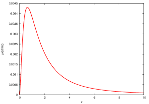
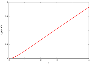
In the previous sections, the Chapman-Enskog method was used in order to obtain first order approximation to the transport coefficients of a two-dimensional relativistic gas from the complete Boltzmann equation. The analytical expressions obtained in terms of collision brackets are general and can be evaluated for particular models of molecular interactions. Explicit values for the thermal and viscous coefficients were established in Sects. 5-7 for the particular case of a hard disks system. The functional behavior of these are plotted in Fig. (1), where $L_{T}$ and $L_{nT}$ are normalized to the non-relativistic thermal conductivity and $\mu$ and $\eta$ to the non-relativistic shear viscosity.

Figure 1: The transport coefficients $\mu/\eta_{\left(NR\right)}$, $\eta/\eta_{\left(NR\right)}$, $L_{T}/L_{T(NR)}$ and $L_{nT}/L_{T(NR)}$ from left to right - up to down, respectively.

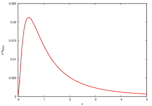
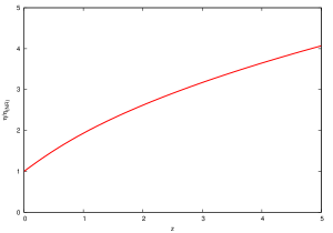
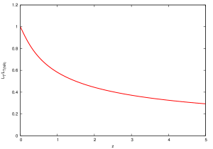
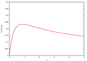
Qualitatively one can clearly observe that the non-relativistic limits are satisfied with, $\mu/\eta{}_{\left(NR\right)}\rightarrow 0$, $\eta/\eta{}_{\left(NR\right)}\rightarrow 0$, $L_{T}/L_{T\left(NR\right)}\rightarrow 1$ and $L_{nT}/L_{T\left(NR\right)}\rightarrow 0$. Moreover, since in the limit $z\rightarrow 0$, one can approximate

$$\mathcal{I}_{2}\sim\int_{2/z}^{\infty}e^{-\left(x-\frac{2}{z}\right)}x\left(z^{2}x^{2}-4\right)^{5/2}dx=240e^{\frac{2}{z}}z\mathcal{K}_{4}\left(\frac{1}{z}\right),$$

$$\mathcal{I}_{3}\sim\int_{2/z}^{\infty}e^{-\left(x-\frac{2}{z}\right)}\left(z^{2}x^{2}-4\right)^{5/2}dx=120e^{\frac{2}{z}}z^{2}\mathcal{K}_{3}\left(\frac{1}{z}\right),$$

where $\mathcal{K}_{n}$ denotes the $n-th$ order modified Bessel function of the second kind, one has

$$L_{T}\sim L_{T\left(\text{NR}\right)}\left(1-\frac{105}{48}z+\frac{4515}{1536}z^{2}....\right),$$

$$\eta\sim\eta_{\left(\text{NR}\right)}\left(1-\frac{63}{16}z+\frac{4473}{512}z^{2}....\right).$$

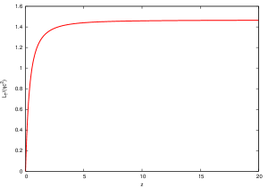
The vanishing at mild and low temperatures of $\mu$ and $L_{nT}$ for the single component monoatomic gas is a known fact which can be corroborated for example in Ref. Ch-E . In Fig. (2) one can verify that these coefficients vanish by themselves thus recovering the Fourier and Navier-Newton relations for these kind of systems at the low temperature limits. The rigorous examination of these limits as well as the analysis of the relation of these coefficients with those obtained by Miller et. al. millerUR using a relaxation approximation and the method of moments deserves a separate discussion which will be published elsewhere. However, it is worthwhile to notice at this stage that the bulk viscosity tends to zero and the ratio $L_{T}/\eta$ approaches a constant value (in dimensionless variables) for large values of $z$, in agreement with the general results in such work (see Fig. (3)).

Figure 2: The dimensionless bulk viscosity $\mu$ and the coefficient $L_{nT}$ as functions of the relativistic parameter $z.$

Figure 3: The ratio $L_{T}/\left(\eta c^{2}\right)$ approaching a constant value (in dimensionless variables) for large values of $z$.

Appendix A Appendix A

In this appendix, the establishment of the expressions for the integrals of the form $\mathcal{T}_{n}^{\alpha_{1}...\alpha_{n}}=\int f^{\left(0\right)}A\left(\gamma\right)v^{\alpha_{1}}v^{\alpha_{2}}...v^{\alpha_{n}}dv^{*}$, for any integrable function $A\left(\gamma\right)$, is shown to some detail for $n=1-4$. These results are used throughout the main text. The procedure in all cases consists in expressing the molecular velocity as $v^{\alpha}=v^{\beta}h_{\beta}^{\alpha}+\gamma u^{\alpha}$ together with the transformation equation Ref. Micro

$$v^{\alpha}=\mathcal{L}^{\alpha\beta}K_{\beta}.$$ (81)

Here $\mathcal{L}^{\alpha\beta}$ is a Lorentz boost to a system moving with velocity $\vec{w}$, and thus with the fluid element, and $K_{\beta}$ is the molecule’s four velocity in such a frame, namely the chaotic velocity. One then has, for $n=1$:

$$\int A\left(\gamma\right)v^{\alpha}dv^{*}=\int A\left(\gamma\right)h_{\beta}^{\alpha}v^{\beta}dv^{*}+2\pi c^{2}u^{\alpha}\int A\left(\gamma\right)\gamma d\gamma,$$ (82)

and since

$$\int A\left(\gamma\right)h_{\beta}^{\alpha}v^{\beta}dv^{*}=h_{\beta}^{\alpha}\mathcal{L}_{\mu}^{\beta}\int A\left(\gamma\right)K^{\mu}dv^{*}=h_{\beta}^{\alpha}\mathcal{L}_{i}^{\beta}\int A\left(\gamma\right)K^{i}dv^{*}=0,$$ (83)

thus

$$\int A\left(\gamma\right)v^{\alpha}dv^{*}=2\pi c^{2}u^{\alpha}\int A\left(\gamma\right)\gamma d\gamma.$$ (84)

Similarly, for $n=2$,

$$\int A\left(\gamma\right)v^{\mu}v^{\nu}dv^{*} =u^{\nu}u^{\mu}\int\gamma^{2}A\left(\gamma\right)dv^{*}+u^{\mu}h_{\delta}^{\nu}\int\gamma A\left(\gamma\right)v^{\delta}dv^{*}$$ (85)

$$+u^{\nu}h_{\sigma}^{\mu}\int\gamma A\left(\gamma\right)v^{\sigma}dv^{*}+\int A\left(\gamma\right)\left(h_{\delta}^{\nu}h_{\sigma}^{\mu}v^{\delta}v^{\sigma}\right)dv^{*},$$

where the second and third terms vanish in view of Eq. (84). For the last term we use Eq. (81), by means of which one obtains

$$\int A\left(\gamma\right)\left(h_{\delta}^{\nu}h_{\sigma}^{\mu}v^{\delta}v^{\sigma}\right)dv^{*} =h_{\delta}^{\nu}h_{\sigma}^{\mu}\mathcal{L}_{i}^{\sigma}\mathcal{L}^{\delta j}\int A\left(\gamma\right)\left(K^{i}K_{j}\right)dv^{*}$$ (86)

$$=-h_{\delta}^{\nu}h_{\sigma}^{\mu}\mathcal{L}_{i}^{\sigma}\mathcal{L}^{\delta j}\delta_{j}^{i}\int A\left(\gamma\right)\gamma^{2}\frac{k^{2}}{2}dv^{*},$$

where, for the second equality, we have used the isotropy in the phase space integral to write

$$\int A\left(\gamma\right)\gamma^{2}\left(k^{1}k_{1}\right)dk^{*}=\int A\left(\gamma\right)\gamma^{2}\left(k^{2}k_{2}\right)dk^{*}=-\frac{1}{2}\int A\left(\gamma\right)\gamma^{2}k^{2}dk^{*}.$$ (87)

Finally, since $\gamma^{2}k^{2}=-c^{2}\left(1-\gamma^{2}\right)$

$$\int A\left(\gamma\right)v^{\mu}v^{\nu}dv^{*}=2\pi c^{4}\left\{\frac{u^{\mu}u^{\nu}}{c^{2}}\int\gamma^{2}A\left(\gamma\right)d\gamma+\frac{1}{2}h^{\mu\nu}\int\left(1-\gamma^{2}\right)A\left(\gamma\right)d\gamma\right\}.$$ (88)

The integral corresponding to $n=3$ can be reduced to

$$\int A\left(\gamma\right)v^{\mu}v^{\nu}v^{\sigma}dv^{*} = 2\pi c^{2}u^{\mu}u^{\nu}u^{\sigma}\int A\left(\gamma\right)\gamma^{3}d\gamma+h_{\alpha}^{\mu}h_{\beta}^{\nu}h_{\delta}^{\sigma}\int A\left(\gamma\right)v^{\alpha}v^{\beta}v^{\delta}dv^{*}$$ (89)

$$+ u^{\sigma}h_{\alpha}^{\mu}h_{\beta}^{\nu}\int A\left(\gamma\right)\gamma v^{\alpha}v^{\beta}dv^{*}+u^{\nu}h_{\alpha}^{\mu}h_{\delta}^{\sigma}\int A\left(\gamma\right)\gamma v^{\alpha}v^{\delta}dv^{*}$$

$$+ u^{\mu}h_{\beta}^{\nu}h_{\delta}^{\sigma}\int A\left(\gamma\right)\gamma v^{\delta}v^{\beta}dv^{*},$$

since various terms featuring $v^{\alpha}$ in the integrand vanish as in the previous case. The second term in Eq. (89) also vanishes since

$$h_{\alpha}^{\mu}h_{\beta}^{\nu}h_{\delta}^{\sigma}\int A\left(\gamma\right)v^{\alpha}v^{\beta}v^{\delta}dv^{*}=h_{\alpha}^{\mu}h_{\beta}^{\nu}h_{\delta}^{\sigma}\mathcal{L}_{\lambda}^{\alpha}\mathcal{L}_{\epsilon}^{\beta}\mathcal{L}_{\chi}^{\delta}\int A\left(\gamma\right)\gamma^{3}k^{\lambda}k^{\epsilon}k^{\chi}dv^{*}=0,$$ (90)

and for the rest of the integrals one uses Eq. (88), leading to

$$u^{\sigma}h_{\alpha}^{\mu}h_{\beta}^{\nu}\int A\left(\gamma\right)\gamma v^{\alpha}v^{\beta}dv^{*} = 2\pi c^{4}u^{\sigma}h_{\alpha}^{\mu}h_{\beta}^{\nu}\int A\left(\gamma\right)\left[\frac{u^{\alpha}u^{\beta}}{c^{2}}\gamma^{3}+\frac{1}{2}h^{\alpha\beta}\gamma\left(1-\gamma^{2}\right)\right]d\gamma$$ (91)

$$= 2\pi c^{4}\frac{1}{2}u^{\sigma}h^{\mu\nu}\int A\left(\gamma\right)\gamma\left(1-\gamma^{2}\right)d\gamma,$$

and analogous expressions for the remaining two terms. Using such results one is led to the following expression

$$\int A\left(\gamma\right)v^{\mu}v^{\nu}v^{\sigma}dv^{*} = 2\pi c^{5}\left\{\frac{u^{\mu}u^{\nu}u^{\sigma}}{c^{3}}\int A\left(\gamma\right)\gamma^{3}d\gamma\right.$$ (92)

$$\left.+\frac{1}{2c}\left(h^{\mu\nu}u^{\sigma}+h^{\mu\sigma}u^{\nu}+h^{\nu\sigma}u^{\mu}\right)\int A\left(\gamma\right)\gamma\left(1-\gamma^{2}\right)d\gamma\right\}.$$

Finally, in order to address the case $n=4$, we use Eq. (90) which reduces the integral to the following three terms

$$\int A\left(\gamma\right)v^{\mu}v^{\nu}v^{\sigma}v^{\lambda}dv^{*} = 2\pi c^{2}u^{\mu}u^{\nu}u^{\sigma}u^{\lambda}\int A\left(\gamma\right)\gamma^{4}d\gamma+h_{\alpha}^{\mu}h_{\beta}^{\nu}h_{\delta}^{\sigma}h_{\epsilon}^{\lambda}\int A\left(\gamma\right)v^{\alpha}v^{\beta}v^{\delta}v^{\epsilon}dv^{*}$$ (93)

$$+ \pi c^{4}\left(u^{\sigma}u^{\lambda}h^{\mu\nu}+u^{\nu}u^{\lambda}h^{\mu\sigma}+u^{\mu}u^{\lambda}h^{\nu\sigma}+u^{\sigma}u^{\nu}h^{\mu\lambda}\right.$$

$$+ \left.u^{\sigma}u^{\mu}h^{\nu\lambda}+u^{\mu}u^{\nu}h^{\lambda\sigma}\right)\int A\left(\gamma\right)\gamma^{2}\left(1-\gamma^{2}\right)d\gamma.$$

For the second term, one can write

$$h_{\alpha}^{\mu}h_{\beta}^{\nu}h_{\delta}^{\sigma}h_{\epsilon}^{\lambda}\int A\left(\gamma\right)v^{\alpha}v^{\beta}v^{\delta}v^{\epsilon}dv^{*}=h_{\alpha}^{\mu}h_{\beta}^{\nu}h_{\delta}^{\sigma}h_{\epsilon}^{\lambda}\mathcal{L}_{a}^{\alpha}\mathcal{L}_{b}^{\beta}\mathcal{L}_{c}^{\delta}\mathcal{L}_{d}^{\epsilon}\int\gamma^{7}A\left(\gamma\right)k^{a}k^{b}k^{c}k^{d}d^{2}k$$ (94)

with $a,\,b,\,c,\,d=1,2$ and $d^{2}k=kdkd\theta$. Integrating over $\theta$ and using $\mathcal{L}_{i}^{\sigma}\mathcal{L}^{\delta j}\delta_{j}^{i}=\mathcal{L}_{i}^{\sigma}\mathcal{L}^{\delta i}=h^{\sigma\delta}$ yields

$$h_{\alpha}^{\mu}h_{\beta}^{\nu}h_{\delta}^{\sigma}h_{\epsilon}^{\lambda}\int A\left(\gamma\right)v^{\alpha}v^{\beta}v^{\delta}v^{\epsilon}dv^{*}=\frac{\pi c^{6}}{4}\left(h^{\mu\nu}h^{\sigma\lambda}+h^{\mu\lambda}h^{\nu\sigma}+h^{\mu\sigma}h^{\nu\lambda}\right)\int A\left(\gamma\right)\left(\gamma^{2}-1\right)^{2}d\gamma,$$ (95)

and thus

$$\int A\left(\gamma\right)v^{\mu}v^{\nu}v^{\sigma}v^{\lambda}dv^{*} = \pi c^{6}\left\{\frac{1}{4}\left(h^{\mu\nu}h^{\sigma\lambda}+h^{\mu\lambda}h^{\nu\sigma}+h^{\mu\sigma}h^{\nu\lambda}\right)\int A\left(\gamma\right)\left(\gamma^{2}-1\right)^{2}d\gamma\right.$$ (96)

$$+ \frac{1}{c^{2}}\left(u^{\sigma}u^{\lambda}h^{\mu\nu}+u^{\nu}u^{\lambda}h^{\mu\sigma}+u^{\mu}u^{\lambda}h^{\nu\sigma}+u^{\sigma}u^{\nu}h^{\mu\lambda}+u^{\sigma}u^{\mu}h^{\nu\lambda}+u^{\mu}u^{\nu}h^{\lambda\sigma}\right)$$

$$\times \left.\int\gamma^{2}\left(1-\gamma^{2}\right)A\left(\gamma\right)d\gamma+\frac{2}{c^{4}}u^{\mu}u^{\nu}u^{\sigma}u^{\lambda}\int\gamma^{4}A\left(\gamma\right)d\gamma\right\}.$$

Appendix B Appendix B

In order to reduce the proposed general solution given in Eq. (30) to the one stated in Eq. (33), one starts by writing $\mathcal{A}_{\alpha\beta}$ in a general way, in terms of all the symmetric second rank tensors

$$\mathcal{A}_{\alpha\beta}=a\eta_{\alpha\beta}+bu_{\alpha}u_{\beta}+d\left(v_{\alpha}u_{\beta}+v_{\beta}u_{\alpha}\right)+ev_{\alpha}v_{\beta},$$ (97)

since any antisymmetrical component would vanish upon contraction with $\mathring{\sigma}^{\alpha\beta}$. Also, since $\mathring{\sigma}^{\alpha\beta}$ is orthogonal to both $u^{\alpha}$ and $u^{\beta}$, $b$ and $d$ can be chosen to be zero. Similarly one can consider $a=0$ since $\mathring{\sigma}^{\alpha\beta}\eta_{\alpha\beta}=0$. Thus, by renaming $e=A_{4}\left(\gamma_{k}\right)$, the term in Eq. (30) corresponding to the traceless symmetric part of the velocity gradient is given solely by $A_{4}\left(\gamma_{k}\right)v_{\alpha}v_{\beta}\mathring{\sigma}^{\alpha\beta}$.

In order to impose the subsidiary conditions, we start by rewriting Eq. (31) as

$$\int\left[\left(\mathcal{A}_{1}\left(\gamma_{k}\right)\frac{T_{,\alpha}}{T}+\mathcal{A}_{2}\left(\gamma_{k}\right)\frac{n_{,\alpha}}{n}\right)v^{\beta}h_{\beta}^{\alpha}+\mathcal{A}_{3}\left(\gamma_{k}\right)u_{,\alpha}^{\alpha}\right.\left.+A_{4}\left(\gamma_{k}\right)v_{\alpha}v_{\beta}\mathring{\sigma}^{\alpha\beta}+\alpha+\check{\alpha}_{\alpha}v^{\alpha}\right]\gamma_{k}^{2}f^{(0)}d\gamma_{k}=0.$$ (98)

Using the integrals (83) and (88) given in Appendix A and since $\mathring{\sigma}^{\alpha\beta}h_{\alpha\beta}=0$, the previous equation can be reduced to

$$\int\left[\left(\mathcal{A}_{3}\left(\gamma_{k}\right)u_{,\alpha}^{\alpha}+\alpha\right)\gamma_{k}^{2}+\check{\alpha}_{\alpha}u^{\alpha}\gamma_{k}^{3}\right]f^{\left(0\right)}d\gamma_{k}=0.$$ (99)

Similarly, using again Appendix A, one can show that Eq. (32) can be written as

$$\int\left\{c^{2}h^{\mu\alpha}\left(1-\gamma_{k}^{2}\right)\left(\mathcal{A}_{1}\left(\gamma_{k}\right)\frac{T_{,\alpha}}{T}+\mathcal{A}_{2}\left(\gamma_{k}\right)\frac{n_{,\alpha}}{n}+\check{\alpha}_{\alpha}\right)\right.$$ (100)

$$\left.+2u^{\mu}\left[\left(\mathcal{A}_{3}\left(\gamma_{k}\right)u_{,\alpha}^{\alpha}+\alpha\right)\gamma_{k}+\check{\alpha}_{\alpha}u^{\alpha}\gamma_{k}^{2}\right]\right\} f^{\left(0\right)}d\gamma_{k}=0.$$

Separating the parallel and orthogonal components with respect to $u^{\mu}$ one obtains two independent conditions namely,

$$h^{\mu\alpha}\int f^{\left(0\right)}\left(1-\gamma_{k}^{2}\right)\left(\mathcal{A}_{1}\left(\gamma_{k}\right)\frac{T_{,\alpha}}{T}+\mathcal{A}_{2}\left(\gamma_{k}\right)\frac{n_{,\alpha}}{n}+\check{\alpha}_{\alpha}\right)d\gamma_{k}=0,$$ (101)

and

$$\int f^{\left(0\right)}\left[\left(\mathcal{A}_{3}\left(\gamma_{k}\right)u_{,\alpha}^{\alpha}+\alpha\right)\gamma_{k}+\check{\alpha}_{\alpha}u^{\alpha}\gamma_{k}^{2}\right]d\gamma_{k}=0.$$ (102)

From Eqs. (99) and (102) one can readily deduce that both $\alpha$ and$\check{\alpha}_{\alpha}u^{\alpha}$ are proportional to $u_{,\alpha}^{\alpha}$ and thus can be omitted. On the other hand, $h^{\mu\alpha}\check{\alpha}_{\alpha}$ can also be omitted, by means of Eq. (101), and thus the solution to be proposed can be simplified in order to read

$$\phi\left(v^{\nu}\right)=\left(A_{1}\left(\gamma_{k}\right)\frac{T_{,\alpha}}{T}+A_{2}\left(\gamma_{k}\right)\frac{n_{,\alpha}}{n}\right)v^{\beta}h_{\beta}^{\alpha}+A_{3}\left(\gamma_{k}\right)u_{,\alpha}^{\alpha}+A_{4}\left(\gamma_{k}\right)v_{\alpha}v_{\beta}\mathring{\sigma}^{\alpha\beta},$$ (103)

and the subsidiary conditions are reduced to

$$h^{\mu\alpha}\int\left(1-\gamma_{k}^{2}\right)\left(A_{1}\left(\gamma_{k}\right)\frac{T_{,\alpha}}{T}+A_{2}\left(\gamma_{k}\right)\frac{n_{,\alpha}}{n}\right)f^{\left(0\right)}d\gamma_{k}=0,$$ (104)

and

$$\int A_{3}\left(\gamma\right)\gamma_{k}f^{\left(0\right)}d\gamma_{k}=\int A_{3}\left(\gamma_{k}\right)\gamma_{k}^{2}f^{\left(0\right)}d\gamma_{k}=0.$$ (105)

Appendix C Appendix C

As mentioned above, the values for the coefficients $\alpha_{nj}^{(i)}$ required in this work are obtained by a standard Gram-Schmidt procedure with the weight functions $p^{\left(1\right)}\left(z\right)=p^{\left(2\right)}\left(z\right)=e^{-\frac{\gamma}{z}}\left(1-\gamma^{2}\right)$, $p^{\left(3\right)}\left(z\right)=e^{-\frac{\gamma}{z}}$ and $p^{\left(4\right)}\left(z\right)=e^{-\frac{\gamma}{z}}\left(1-\gamma^{2}\right)^{2}$. By performing the corresponding calculations one can directly obtain the following expressions

$$\alpha_{11}^{\left(1\right)}=\alpha_{11}^{\left(2\right)}=\sqrt{\frac{\left(z+1\right)e^{1/z}}{2z^{4}\left(3z^{2}+6z+2\right)}},$$ (106)

$$\alpha_{10}^{(1)}=\alpha_{10}^{(2)}=-\sqrt{\frac{\left(z+1\right)e^{1/z}}{2z^{4}\left(3z^{2}+6z+2\right)}}\frac{1+3z+2z^{2}}{1+z},$$ (107)

$$\alpha_{00}^{\left(3\right)}=\sqrt{\frac{e^{1/z}}{z}},$$ (108)

$$\alpha_{10}^{\left(3\right)}=-\sqrt{\frac{e^{1/z}}{z}}\frac{\left(1+z\right)}{z},$$ (109)

$$\alpha_{11}^{\left(3\right)}=\sqrt{\frac{e^{1/z}}{z}}\frac{1}{z},$$ (110)

$$\alpha_{20}^{\left(3\right)}=\sqrt{\frac{e^{1/z}}{z}}\frac{1}{2z^{2}}\left(2z^{2}+4z+1\right),$$ (111)

$$\alpha_{21}^{\left(3\right)}=-\sqrt{\frac{e^{1/z}}{z}}\frac{\left(1+2z\right)}{z^{2}},$$ (112)

$$\alpha_{22}^{\left(3\right)}=\sqrt{\frac{e^{1/z}}{z}}\frac{1}{2z^{2}},$$ (113)

$$\alpha_{00}^{\left(4\right)}=\sqrt{\frac{e^{1/z}}{8z^{2}\left(3z^{2}+3z+1\right)}}.$$ (114)

Appendix D Appendix D

In this appendix, the collision brackets $\left[\gamma^{2},\gamma^{2}\right]$, $\left[\gamma v^{\alpha},\gamma v_{\alpha}\right]$ and $\left[v^{\alpha}v^{\beta},v_{\alpha}v_{\beta}\right]$ are calculated to some detail. Starting from the general definition

$$\left[G,H\right]=-\frac{1}{n^{2}}\int G\left[H^{\prime}_{1}+H^{\prime}-H_{1}-H\right]f^{\left(0\right)}f_{1}^{\left(0\right)}F\sigma\left(Q,\chi\right)d\chi dv_{1}^{*}dv^{*},$$ (115)

the brackets can be written as

$$\left[\gamma^{2},\gamma^{2}\right]=-\frac{1}{n^{2}}\int f^{\left(0\right)}f_{1}^{\left(0\right)}\gamma^{2}\left(\gamma{}_{1}^{{}^{\prime}2}+\gamma{}^{{}^{\prime}2}-\gamma_{1}^{2}-\gamma{}^{2}\right)F\sigma\left(Q,\chi\right)d\chi dv^{*}dv_{1}^{*},$$ (116)

$$\left[\gamma v_{\beta},\gamma v^{\beta}\right]=-\frac{1}{n^{2}}\int f^{\left(0\right)}f_{1}^{\left(0\right)}\gamma v_{\beta}\left(\gamma{}_{1}^{{}^{\prime}}v_{1}^{{}^{\prime}\beta}+\gamma^{{}^{\prime}}v^{{}^{\prime}\beta}-\gamma{}_{1}v_{1}^{\beta}-\gamma v^{\beta}\right)F\sigma\left(Q,\chi\right)d\chi dv^{*}dv_{1}^{*},$$ (117)

$$\left[v_{\alpha}v_{\beta},v^{\alpha}v^{\beta}\right]=-\frac{1}{n^{2}}\int f^{\left(0\right)}f_{1}^{\left(0\right)}v_{\alpha}v_{\beta}\left[v_{1}^{{}^{\prime}\alpha}v{}_{1}^{{}^{\prime}\beta}+v{}^{{}^{\prime}\alpha}v{}^{{}^{\prime}\beta}-v{}_{1}^{\alpha}v{}_{1}^{\beta}-v{}^{\alpha}v{}^{\beta}\right]F\sigma\left(Q,\chi\right)d\chi dv^{*}dv_{1}^{*}.$$ (118)

Introducing the change of variables

$$P^{\alpha}=v^{\alpha}+v_{1}^{\alpha}\qquad Q^{\alpha}=v^{\alpha}-v_{1}^{\alpha},$$

momentum conservation implies

$$P^{\alpha^{\prime}}=P^{\alpha},$$

and choosing the center of mass frame, where $\left(P^{\alpha}\right)=\left(P^{0},0,0\right)$, one can rewrite Eqs. (116-118) as follows

$$\left[\gamma^{2},\gamma^{2}\right]=-\frac{u_{\mu}u_{\beta}u_{\alpha}u_{\nu}}{16c^{7}n^{2}}\int f^{\left(0\right)}f_{1}^{\left(0\right)}\left(P^{\mu}P^{\beta}+P^{\mu}Q^{\beta}+Q^{\mu}P^{\beta}+Q^{\mu}Q^{\beta}\right)\left(Q^{\prime\nu}Q^{\prime\alpha}-Q^{\alpha}Q^{\nu}\right)d\vartheta,$$ (119)

$$\left[\gamma v_{\beta},\gamma v^{\beta}\right]=-\frac{u_{\alpha}u_{\mu}}{16c^{3}n^{2}}\int f^{\left(0\right)}f_{1}^{\left(0\right)}\left(P^{\mu}P_{\beta}+P^{\mu}Q_{\beta}+Q^{\mu}P_{\beta}+Q^{\mu}Q_{\beta}\right)\left(Q^{\prime\beta}Q^{\prime\alpha}-Q^{\beta}Q^{\alpha}\right)d\vartheta,$$ (120)

$$\left[v_{\alpha}v_{\beta},v^{\alpha}v^{\beta}\right]=-\frac{c}{16n^{2}}\int f^{\left(0\right)}f_{1}^{\left(0\right)}\left(P_{\alpha}P_{\beta}+P_{\alpha}Q_{\beta}+Q_{\alpha}P_{\beta}+Q_{\alpha}Q_{\beta}\right)\left(Q^{\prime\beta}Q^{\prime\alpha}-Q^{\beta}Q^{\alpha}\right)d\vartheta,$$ (121)

where $d\vartheta=\sigma\left(\chi\right)d\chi\left(Q/P^{0}\right)d^{2}Pd^{2}Q$ and $Q^{\alpha}Q_{\alpha}=-Q^{2}$. The scattering cross section for hard disks is given by

$$\sigma\left(\chi\right)=\frac{d}{2}\left|\sin\left(\frac{\chi}{2}\right)\right|,$$

where $\chi$ represents the scattering angle. If the $x_{2}$ axis is aligned in the $Q^{\alpha}$ direction one has

$$Q^{\alpha}=\left(\begin{array}[]{c}0\\ 0\\ 1\end{array}\right)\qquad Q^{{}^{\prime}\alpha}=\left(\begin{array}[]{c}0\\ \sin\chi\\ \cos\chi\end{array}\right),$$

which leads to

$$\int_{0}^{2\pi}\left(Q^{{}^{\prime}\mu}Q^{{}^{\prime}\beta}-Q^{\mu}Q^{\beta}\right)\sigma\left(\chi\right)d\chi=\frac{16d}{15}Q^{2}\left[\frac{P^{\mu}P^{\beta}}{P^{2}}-\eta^{\mu\beta}-2\frac{Q^{\mu}Q^{\beta}}{Q^{2}}\right],$$

where $d$ is the diameter of the disks. Introducing this result in Eqs. (119-121) yields

$$\left[\gamma^{2},\gamma^{2}\right]=-\frac{du_{\mu}u_{\beta}u_{\alpha}u_{\nu}}{15c^{7}n^{2}}\int f^{\left(0\right)}f_{1}^{\left(0\right)}\left(P^{\mu}P^{\beta}+P^{\mu}Q^{\beta}+Q^{\mu}P^{\beta}+Q^{\mu}Q^{\beta}\right)\chi^{\nu\alpha}\frac{Q^{3}}{P^{0}}d^{2}Pd^{2}Q,$$ (122)

$$\left[\gamma v_{\beta},\gamma v^{\beta}\right]=-\frac{du_{\alpha}u_{\mu}}{15c^{3}n^{2}}\int f^{\left(0\right)}f_{1}^{\left(0\right)}\left(P^{\mu}P_{\beta}+P^{\mu}Q_{\beta}+Q^{\mu}P_{\beta}+Q^{\mu}Q_{\beta}\right)\chi^{\beta\alpha}\frac{Q^{3}}{P^{0}}d^{2}Pd^{2}Q,$$ (123)

$$\left[v_{\alpha}v_{\beta},v^{\alpha}v^{\beta}\right]=-\frac{dc}{15n^{2}}\int f^{\left(0\right)}f_{1}^{\left(0\right)}\left(P_{\alpha}P_{\beta}+P_{\alpha}Q_{\beta}+Q_{\alpha}P_{\beta}+Q_{\alpha}Q_{\beta}\right)\chi^{\beta\alpha}\frac{Q^{3}}{P^{0}}d^{2}Pd^{2}Q,$$ (124)

where we have defined

$$\chi^{\nu\alpha}=\left[\frac{P^{\nu}P^{\alpha}}{P^{2}}-\eta^{\nu\alpha}-2\frac{Q^{\nu}Q^{\alpha}}{Q^{2}}\right].$$ (125)

In order to calculate the integrals in the polar angle we use

$$\left(Q^{\alpha}\right)=Q\left(\begin{array}[]{c}0\\ \cos\phi\\ \sin\phi\end{array}\right),\qquad d^{2}Q=Qd\phi dQ$$

and after a somewhat lengthy procedure, one can obtain

$$\left[\gamma^{2},\gamma^{2}\right]=\frac{\pi d\zeta\left(z\right)^{2}}{30c^{7}}\int e^{-\frac{u_{\alpha}P^{\alpha}}{zc^{2}}}u_{\alpha}u_{\beta}\left[u_{\mu}u_{\nu}\frac{P^{\alpha}P^{\beta}P^{\mu}P^{\nu}}{P^{4}}-2c^{2}\frac{P^{\alpha}P^{\beta}}{P^{2}}+c^{2}\eta^{\alpha\beta}\right]\frac{Q^{6}}{P^{0}}d^{2}PdQ,$$ (126)

$$\left[\gamma v_{\beta},\gamma v^{\beta}\right]=-\frac{\pi d\zeta\left(z\right)^{2}}{15c^{3}}\int e^{-\frac{u_{\alpha}P^{\alpha}}{zc^{2}}}u_{\mu}u_{\alpha}\left[\frac{P^{\alpha}P^{\mu}}{P^{2}}-\eta^{\alpha\mu}\right]\frac{Q^{6}}{P^{0}}d^{2}PdQ,$$ (127)

$$\left[v_{\alpha}v_{\beta},v^{\alpha}v^{\beta}\right]=\frac{2\pi d\zeta\left(z\right)^{2}}{15c^{-1}}\int e^{-\frac{u_{\alpha}P^{\alpha}}{zc^{2}}}\frac{Q^{6}}{P^{0}}d^{2}PdQ.$$ (128)

with $\zeta\left(z\right)=\left(1/2\pi c^{2}\right)\left(e^{1/z}/\left(z+z^{2}\right)\right)$. Now we can identify the following functions in the above equations,

$$Z^{*}=\int e^{-\frac{U_{\alpha}P^{\alpha}}{zc^{2}}}\frac{d^{2}P}{P^{0}},$$ (129)

$$Z_{\mu\alpha}^{*}=\int e^{-\frac{U_{\alpha}P^{\alpha}}{zc^{2}}}P_{\alpha}P_{\mu}\frac{d^{2}P}{P^{0}},$$ (130)

$$Z_{\alpha\beta\mu\nu}^{*}=\int e^{-\frac{U_{\alpha}P^{\alpha}}{zc^{2}}}P_{\alpha}P_{\beta}P_{\mu}P_{\nu}\frac{d^{2}P}{P^{0}},$$ (131)

and rewrite Eqs. (126-128) as

$$\left[\gamma^{2},\gamma^{2}\right]=\frac{\pi d}{30c^{7}}\zeta\left(z\right)^{2}\int\left(\frac{u_{\alpha}u_{\beta}u_{\mu}u_{\nu}}{P^{4}}Z_{\alpha\beta\mu\nu}^{*}-2c^{2}\frac{u_{\alpha}u_{\beta}}{P^{2}}Z_{\alpha\beta}^{*}+c^{4}Z^{*}\right)Q^{6}dQ,$$ (132)

$$\left[\gamma v_{\beta},\gamma v^{\beta}\right]=-\frac{d\pi}{15c^{3}}\zeta\left(z\right)^{2}\int\left(\frac{u_{\mu}u_{\alpha}}{P^{2}}Z_{\mu\alpha}^{*}-c^{2}Z^{*}\right)Q^{6}dQ,$$ (133)

$$\left[v_{\alpha}v_{\beta},v^{\alpha}v^{\beta}\right]=\frac{2\pi d}{15c^{-1}}\zeta\left(z\right)^{2}\int Z^{*}Q^{6}dQ.$$ (134)

The integrals in Eqs. (129-131) are evaluated in some detail in Ref. HFBidi following the procedure shown in Ref. CercignaniKremer , which yield

$$Z^{*}=2\pi cz\exp\left(-\frac{\mathcal{Q}}{z}\right),$$

$$u^{\mu}u^{\alpha}Z_{\mu\alpha}^{*}=2\pi c^{5}z\exp\left(-\frac{\mathcal{Q}}{z}\right)\left[\mathcal{Q}^{2}+2\mathcal{Q}z+2z^{2}\right],$$

$$u^{\alpha}u^{\beta}u^{\mu}u^{\nu}Z_{\alpha\beta\mu\nu}^{*}=2\pi c^{9}z\exp\left(-\frac{\mathcal{Q}}{z}\right)\left[12\mathcal{Q}^{2}z^{2}+24\mathcal{Q}z^{3}+24z^{4}+4\mathcal{Q}^{3}z+\mathcal{Q}^{4}\right],$$

where we have also used energy-momentum conservation $P^{2}=4c^{2}+Q^{2}$ and the change of variable $Q^{2}+4c^{2}=c^{2}\mathcal{Q}^{2}$. Thus, one can write Eqs. (132-134) as follows

$$\left[\gamma^{2},\gamma^{2}\right]=\frac{2czd}{15}\frac{e^{2/z}}{\left(z+z^{2}\right)^{2}}\int_{2}^{\infty}\exp\left(-\frac{\mathcal{Q}}{z}\right)\left(\frac{z^{2}}{\mathcal{Q}^{2}}+3\frac{z^{3}}{\mathcal{Q}^{3}}+3\frac{z^{4}}{\mathcal{Q}^{4}}\right)\left(\mathcal{Q}^{2}-4\right)^{5/2}\mathcal{Q}d\mathcal{Q},$$ (135)

$$\left[\gamma v_{\beta},\gamma v^{\beta}\right]=-\frac{c^{3}zd}{15}\frac{e^{2/z}}{\left(z+z^{2}\right)^{2}}\int_{2}^{\infty}\exp\left(-\frac{\mathcal{Q}}{z}\right)\left(\frac{z}{\mathcal{Q}}+\frac{z^{2}}{\mathcal{Q}^{2}}\right)\left(\mathcal{Q}^{2}-4\right)^{5/2}\mathcal{Q}d\mathcal{Q},$$ (136)

$$\left[v_{\alpha}v_{\beta},v^{\alpha}v^{\beta}\right]=\frac{c^{5}zd}{15}\frac{e^{2/z}}{\left(z+z^{2}\right)^{2}}\int_{2}^{\infty}\exp\left(-\frac{\mathcal{Q}}{z}\right)\left(\mathcal{Q}^{2}-4\right)^{5/2}\mathcal{Q}d\mathcal{Q}.$$ (137)

and introducing the change of variable $x=\mathcal{Q}/z$ one obtains

$$\left[\gamma^{2},\gamma^{2}\right]=\frac{2cz^{3}d}{15}\frac{e^{2/z}}{\left(z+z^{2}\right)^{2}}\int_{2/z}^{\infty}e^{-x}\left(\frac{1}{x}+\frac{3}{x^{2}}+\frac{3}{x^{3}}\right)\left(z^{2}x^{2}-4\right)^{5/2}dx,$$ (138)

$$\left[\gamma v_{\beta},\gamma v^{\beta}\right]=-\frac{c^{3}z^{3}d}{15}\frac{e^{2/z}}{\left(z+z^{2}\right)^{2}}\int_{2/z}^{\infty}e^{-x}\left(1+\frac{1}{x}\right)\left(z^{2}x^{2}-4\right)^{5/2}dx,$$ (139)

$$\left[v_{\alpha}v_{\beta},v^{\alpha}v^{\beta}\right]=\frac{c^{5}z^{3}d}{15}\frac{e^{2/z}}{\left(z+z^{2}\right)^{2}}\int_{2/z}^{\infty}e^{-x}x\left(z^{2}x^{2}-4\right)^{5/2}dx,$$ (140)

these integrals can be obtained numerically for a given value of $z$.

References

- (1) See for example C. Farías, V. A. Pinto and P. S. Moya. What is the temperature of a moving body? Scientific Reports, volume 7, Article number: 17657 (2017) and references cited therein.
- (2) M. Mendoza, H. J. Herrmann, and S. Succi. Hydrodynamic model for conductivity in graphene. Scientific Reports, 3, 2013.
- (3) M. M. Doria R. C.V. Coelho, M. Mendoza and H. J. Herrmann. Fully dissipative relativistic lattice boltzmann method in two dimensions. Computers and Fluids, in press (2018).
- (4) W. Israel. Relativistic kinetic theory of a simple gas. J. Math. Phys., 4:1163, 1963.
- (5) W. A. van Leeuwen and S. R. de Groot. On relativistic kinetic gas theory: V. the coefficients of heat conductivity, diffusion and thermal diffusion for a binary mixture of relativistic maxwellian molecules. Physica, 51:16–31, 1971.
- (6) W. A. van Leeuwen S. R. de Groot and C. van del Wert. Relativistic Kinertic Theory. North Holand Publ. Co., 1980.
- (7) C. Cercignani and G. Kremer. The relativistic Boltzmann equation: Theory and applications. Cambridge University Press 3rd Ed, 1991.
- (8) A. L. García-Perciante and A. Sandoval-Villalbazo. Remarks on relativistic kinetic theory to first order in the gradients. J. Non Newton. Fluid Mech., 165:1024–1028, 2010.
- (9) M Mendoza, I Karlin, S Succi, and H J Herrmann. Ultrarelativistic transport coefficients in two dimensions. J. Stat. Mech., page P02036, 2013.
- (10) A. L. García-Perciante, A. R. Méndez, and E. Escobar-Aguilar. Heat flux for a relativistic bidimensional gas. J. Stat. Phys., 16:123–134, 2017.
- (11) S. Chapman and T. G. Cowling. The Mathematical Theory of Non-Uniform Gases. Cambridge University Press, 1970.
- (12) M. Ghodrat and A. Montakhab. Heat transport and difussion in a canonical model of a relativistic gas. Phys. Rev. E, 87:032120, 2013.
- (13) C. Eckart. The thermodynamics of irreversible processes. iii. relativistic theory of the simple fluid. Phys. Rev., 58:919, 1940.
- (14) Ch. W. Misner, K. S. Thorne, and J. A. Wheeler. Gravitation. W. H. Freenan and Company San Francisco, 1973.
- (15) Valdemar Moratto and A. L. García-Perciante. On the role of the chaotic velocity in relativistic kinetic theory. AIP Conf. Proc., 1578(86), 2014.
- (16) A.L.García-Perciante, A. Sandoval-Villalbazo, and L.S.García-Colin. On the microscopic nature of dissipative effects in special relativistic kinetic theory. J. Non-Equilib. Thermodyn., 37, 2012.
- (17) J. V. Sengers. Lectures in Theoretical Physics, Kinetic Theory, volume IXC, page 335. Gordon and Breach, New York, 1967.