Dynamical Glass and Ergodization Times in Classical Josephson Junction Chains

Abstract

Models of classical Josephson junction chains turn integrable in the limit of large energy densities or small Josephson energies. Close to these limits the Josephson coupling between the superconducting grains induces a short range nonintegrable network. We compute distributions of finite time averages of grain charges and extract the ergodization time $T_{E}$ which controls their convergence to ergodic $\delta$-distributions. We relate $T_{E}$ to the statistics of fluctuation times of the charges, which are dominated by fat tails. $T_{E}$ is growing anomalously fast upon approaching the integrable limit, as compared to the Lyapunov time $T_{\Lambda}$ - the inverse of the largest Lyapunov exponent - reaching astonishing ratios $T_{E}/T_{\Lambda}\geq 10^{8}$. The microscopic reason for the observed dynamical glass is routed in a growing number of grains evolving over long times in a regular almost integrable fashion due to the low probability of resonant interactions with the nearest neighbors. We conjecture that the observed dynamical glass is a generic property of Josephson junction networks irrespective of their space dimensionality.

Ergodicity is a core concept of statistical physics of many body systems. It demands infinite time averages of observables during a microcanonical evolution to match with their proper phase space averages Lichtenberg and Lieberman (1992). Any laboratory or computational experiment is however constrained to finite averaging times. Are these sufficient or not? How much time is needed for a trajectory to visit the majority of the available microcanonical states, and for the finite-time average of an observable to be reasonably close to its statistical average? Can we define an ergodization time scale $T_{E}$ on which these properties manifest? What is that ergodization time depending on? Doubts on the applicability of the ergodic hypothesis itself were discussed for such simple cases as a mole of Ne at room temperature (see Gaveau and Schulman (2015) and references therein). Glassy dynamics have been reported in a large variety of Hamiltonian systems Biroli and Tarzia (2017); Pérez-Espigares et al. (2018); Tong and Tanaka (2018); Senanian and Narayan (2018). Further, spin-glasses Bouchaud (1992) and stochastic Levy processes Bel and Barkai (2005); Bel, G. and Barkai, E. (2006); Rebenshtok and Barkai (2007, 2008); Korabel and Barkai (2009); Schulz and Barkai (2015) reveal that the ergodization time (and even ergodicity itself) may be affected by heavy-tailed distributions of lifetimes of typical excitations. The aim of this work is to address the above issues using a simple and paradigmatic dynamical many-body system testbed.

Josephson junction networks are devices that are known for their wide applicability over various fields such as superconductivity, cold atoms, optics and meta-materials, among others Cataliotti et al. (2001); Ryu et al. (2013); Cassidy et al. (2017) (for a recent survey on experimental results, see Blackburn et al. (2016)): synchronization has been studied in Ref. Tsygankov and Wiesenfeld (2002); El-Nashar et al. (2003), discrete breathers were observed and studied in Ref. Binder et al. (2000); Miroshnichenko et al. (2001); Fistul et al. (2002); Miroshnichenko et al. (2005), qubit dynamics was analyzed in Ref. Shulga et al. (2018); Martinis (2004) and the thermal conductivity was computed in Ref. Gendelman and Savin (2000); Giardinà et al. (2000). In particular, a recent study conducted by Pino et.al. Pino et al. (2016) showed the existence of a non-ergodic/bad metal region in the high-temperature regime of a quantum chain of Josephson junctions, that exists as a prelude to a many-body localization phase Basko et al. (2006). Notably, in Pino et al. (2016) it has been conjectured that the bad metal regime persists as a non-ergodic phase in the classical limit of the model - the large energy density regime of a chain of coupled rotors, close to an integrable limit. A similar prediction of a nonergodic phase (called weak coupling phase) in the same model was obtained in Escande et al. (1994). Further in De Roeck and Huveneers (2014), a faster decay of thermal conductivity in the high-temperature regime is observed. On the other side, a strong slowing down of relaxations has been identified in the proximity of such a limit if the nonintegrable perturbation spans a short range network between corresponding actions Mithun et al. (2018). The limit of weak Josephson coupling or high temperature is precisely corresponding to that short range network case. Is the Josephson junction chain then ergodic or not?

In this letter we demonstrate the existence of a dynamical glass in a classical Josephson junction chain of coupled rotors. We evaluate the convergence of distributions of finite time averages of the superconducting grain charges, and extract an ergodization time scale $T_{E}$. We show that this time scale is related to the properties of the statistics of charge fluctuation times. Such fluctuation event statistics was introduced in Refs. Danieli et al. (2017); Mithun et al. (2018). We compute the Lyapunov time $T_{\Lambda}$ - the inverse of the largest Lyapunov exponent $\Lambda$ Casetti et al. (1996, 2000). The Lyapunov time is a lower bound for the ergodization time: $T_{\Lambda}\leq T_{E}$. In the reported dynamical glass, the dynamics stays ergodic and $T_{E}$ is finite. However, $T_{E}$ is growing anomalously fast upon approaching the integrable limit, as compared to $T_{\Lambda}$ reaching astonishing ratios $T_{E}/T_{\Lambda}\geq 10^{8}$. We show that $T_{E}$ is controlled by fat tails of charge fluctuation time distributions. We compute the spatio-temporal evolution of nonlinear resonances between interacting grains Livi et al. (1987); Escande et al. (1994). The microscopic reason for the observed dynamical glass is routed in a growing number of grains evolving over long times in a regular almost integrable fashion due to the low probability of resonant interactions with nearest neighbors. The dynamical glass behavior is expected to be a generic property of a large class of dynamical systems, where ergodization time scales depend sensitively on control parameters. At the same time, the concept of ergodicity is preserved, and statistical physics continues to work - it is all just a matter of time scales.

We consider the Hamiltonian

$$\small H(q,p)=\sum_{n=1}^{N}\bigg{[}\frac{p_{n}^{2}}{2}+E_{J}(1-\cos(q_{n+1}-q_{n}))\bigg{]},$$ (1)

describing the dynamics of a chain of $N$ superconducting islands with weak nearest neighbor Josephson coupling in its classical limit. We note that this model is equivalent to an XY chain or similarly to a coupled rotor chain, where the grain charging energies turn into the above kinetic energy terms Livi et al. (1987); Pino et al. (2016). We apply periodic boundary conditions $p_{1}=p_{N+1}$ and $q_{1}=q_{N+1}$ for the conjugate angles $q_{n}$ and momenta $p_{n}$. $E_{J}$ controls the strength of Josephson coupling. The corresponding equations of motion of Eq. (1) are

$$\begin{split}\small\dot{q_{n}}=p_{n},\leavevmode\nobreak\ \leavevmode\nobreak\ \leavevmode\nobreak\ \leavevmode\nobreak\ \dot{p_{n}}&=E_{J}\big{[}\sin(q_{n+1}-q_{n})+\sin(q_{n-1}-q_{n})\big{]}.\end{split}$$ (2)

This system has two conserved quantities: the total energy $H$ and the total angular momentum $L=\sum_{n=1}^{N}p_{n}$. We will choose $L=0$ without loss of generality. Exact expressions for average full $h$ and kinetic $k$ energy densities as functions of temperature are obtained using a Gibbs distribution Sup and yield

$$h=k+E_{J}\left(1-\frac{I_{1}(E_{J}/2k)}{I_{0}(E_{J}/2k)}\right)\;,$$ (3)

with $I_{0,1}$ being the modified Bessel functions of the first kind. We investigate the equilibrium dynamics of the above system in proximity to two integrable limits: $h\rightarrow\infty$, or $E_{J}\rightarrow 0$. At these limits, the system reduces to a set of uncoupled superconducting grains $H_{0}=\sum_{n=1}^{N}\frac{p_{n}^{2}}{2}$ Livi et al. (1987). In proximity to these limits the Josephson terms induce a nonintegrable perturbation through a short-range interaction network of actions $\{p_{n}\}_{n}$ Mithun et al. (2018). We consider the kinetic energies $k_{n}=p_{n}^{2}/2$ as a set of time-dependent observables. Due to the discrete translational invariance of $H$ all $k_{n}$ variables are statistically equivalent, fluctuating around their equilibrium value $k$. We will integrate the equations of motion using symplectic integrators Sup . Unless, otherwise stated, we use the system size $N=2^{10}$.

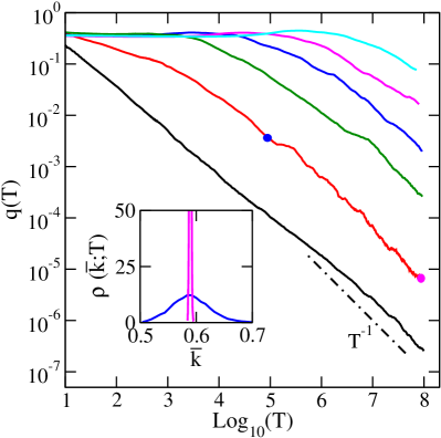
Figure 1: (Color online) a) Fluctuation Index $q(T)$ for energy densities (bottom to top) 0.1 (black) 1.2 (red), 2.4 (green), 3.8 (blue), 5.4 (magenta), and 8.5 (cyan). Inset: $\rho(\overline{k};T)$ for $h=1.2$ and two different times $T=10^{5}$ (blue circle) and $T=10^{8}$ (magenta circle) marked in the main plot. Here $E_{J}=1$ and the number of realizations $R=12$ for all data.

To quantitatively assess the ergodization time $T_{E}$, we compute finite time averages $\overline{k}_{n,T}=\frac{1}{T}\int_{0}^{T}k_{n}(t)dt$ for a set of $R$ different trajectories at given $h,E_{J}$. The corresponding distribution $\rho(\overline{k};T)$ is characterized by its 1st moment $\mu_{k}(T)$ and the standard deviation $\sigma_{k}(T)$. Assuming ergodicity, $\mu_{k}(T\rightarrow\infty)=k$ and $\sigma_{k}(T\rightarrow\infty)=0$, since the distribution $\rho(\overline{k};T\rightarrow\infty)=\delta(\overline{k}-k)$. In the inset of Fig. 1 we show the distributions $\rho(\overline{k};T)$ for $h=1.2$ at two different averaging times $T=10^{5},10^{8}$. As expected the distribution $\rho(\overline{k},T)$ converges to a delta function, centered around $k$. We then use the fluctuation index $q(T)=\frac{\sigma_{k}^{2}(T)}{\mu_{k}^{2}(T)}$ as a quantitative dimensionless measure of the above convergence properties.

In Fig. 1 we show $q(T)$ for different values of $h$ with $E_{J}=1$. We find $q(T\ll T_{E})=q(0)$ and $q(T\gg T_{E})\sim T_{E}/T$ where $T_{E}$ is our definition of the ergodization time scale. We rescale and fit the different curves $q(T)$ and extract $T_{E}$ Sup . The result is plotted in Fig. 3(a) with green squares. $T_{E}$ quickly grows by orders of magnitude upon increasing the energy density $h$ in a rather moderate window of values, close to a power law $T_{E}\sim h^{6}$. When fixing $h=1$ and varying $E_{J}$, we make similar observations Sup , with $T_{E}\sim E_{J}^{-6.5}$ as shown in Fig. 3(b). With our results, we validate ergodic dynamics in the considered system. Previous reports Pino et al. (2016); Escande et al. (1994) were not addressing the quickly growing time scale $T_{E}$ upon approaching the integrable limit.

Figure 2: (Color online) $P_{+}(\tau)$ (solid lines) and $P_{-}(\tau)$ (dashed lines) for various energy densities $h=1.2$ (magenta), $h=2.4$ (blue) and $h=5.4$ (red). Here $E_{J}=1$. The black line corresponds to a power law decay $\tau^{-2}$ and guides the eye. Inset: $\gamma\equiv d(\log_{10}P_{+})/d(\log_{10}\tau)$. The black solid horizontal line guides the eye at value -2.

Let us study the fluctuation statistics of the observables $k_{n}(t)$. Each of them has to fluctuate around their common average $k$. This allows to segment the trajectory of the whole system phase space into consecutive excursions Danieli et al. (2017); Mithun et al. (2018). Note that for each site $n$ the segmenting is different, and we account for all of them. We measure the consecutive piercing times $t_{n}^{i}$ at which $k_{n}(t)=k$. We then compute the excursion times $\tau^{\pm}_{n}(i)=t_{n}^{i+1}-t_{n}^{i}$ for a trajectory of excursion events during which $k(t)>k$ ($\tau^{+}$) and $k(t)<k$ ($\tau^{-}$) respectively. Fig. 2 shows the distributions for $E_{J}=1$ and various energy densities $h$. As $h$ increases both distributions increase their tail weights, with $P_{+}$ dominating over $P_{-}$. Further, the distributions develop intermediate tail structures close to a $1/\tau^{2}$. (inset in Fig.2).

We can now compute the following two time scales: the average excursion time, $\mu_{\tau}$ and the standard deviation $\sigma_{\tau}$ of the distribution $P_{+}$, which are shown in Fig.3(a) (orange diamonds and blue triangles) as functions of $h$. We observe that $\sigma_{\tau}$ equals with $\mu_{\tau}$ at $h\approx 1$ and quickly overgrows $\mu_{\tau}$ for $h>1$, signaling the proximity to an integrable limit, where the dynamics is dominated by fluctuations rather than the means. Indeed, if the distributions $P_{\pm}({\tau})$ asymptotically reach a $1/\tau^{2}$ dependence in the integrable limit, then not only the time scales $\mu_{\tau}$ and $\sigma_{\tau}$ have to diverge, but their ratio $\sigma_{\tau}/\mu_{\tau}$ will diverge as well.

The above time scales are related to the ergodization time scale $T_{E}$ as

$$T_{E}\sim\tau_{q}\equiv\frac{\sigma^{2}_{\tau}}{\mu_{\tau}}.$$ (4)

This relation can be obtained e.g. after approximating the dependence $k_{n}(t)$ by a telegraph random process with excursion time distributions $P_{\pm}$ Sup . We plot $A\tau_{q}$ versus $h$ in Fig.3(a) (black circles) with a fitting parameter $A=130$. The curve is strikingly close to the dependence $T_{E}(h)$ for $h>1$. We thus independently reconfirm that the considered system dynamics is ergodic, yet with quickly growing time scales of ergodization. When fixing $h=1$ and varying $E_{J}$, we make similar observations as shown in Fig. 3(b). The physical origin of $A$ is an interesting and open question for future studies.

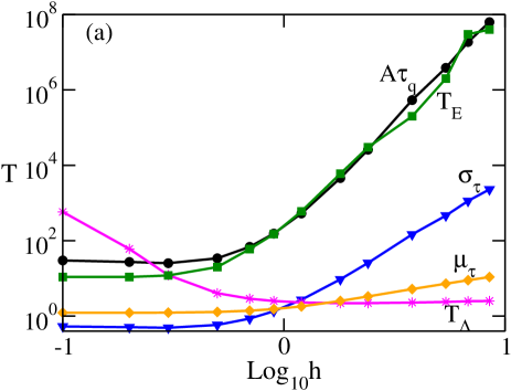
Figure 3: (Color online) (a) Time scales $T_{E}$ (green squares), $A\tau_{q}$ (black circles), Lyapunov time $T_{\Lambda}$ (magenta stars), $\mu_{\tau}$ (orange diamonds) and $\sigma_{\tau}$ (blue triangles) vs the energy density $h$ for $E_{J}=1$ and $A=130$. (b) Same as in (a) but vs $E_{J}$ at the fixed energy density $h=1$. Inset: Rescaled times ($A\tau_{q}$, $T_{E}$, $m_{\tau}$ and $\sigma_{\tau}$) in units of the Lyapunov time $T_{\Lambda}$.

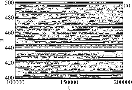
Figure 4: (Color online) (a) Spatiotemporal evolution of a part of the Josephson junction chain for $E_{J}=1$ and $h=5.4$. Black points correspond to events with $k_{n}>k$. (b) Spatiotemporal evolution of nonlinear resonances for the same parameters as in (a). See text for details.

With ergodicity being restored, the question remains: what is the microscopic origin of the enormously fast growing ergodization time? Since the considered system is nonintegrable, its dynamics must be chaotic. Therefore there is a Lyapunov time scale $T_{\Lambda}=1/\Lambda$ dictated by the largest Lyapunov exponent $\Lambda$. $T_{\Lambda}$ can be expected to serve as a lower bound for the ergodization time scale. We compute $\Lambda$ using standard techniques Sup and also compare it with theoretical predictions Casetti et al. (1996, 2000). We plot the Lyapunov time $T_{\Lambda}$ versus $h$ in Fig. 3(a) and versus $E_{J}$ in Fig. 3(b) (magenta stars). The surprising finding is that $T_{\Lambda}\lesssim\mu_{\tau}$ in proximity to the integrable limit. Thus $T_{\Lambda}\ll T_{E}$, e.g. for $E_{J}=1$ and $h=10$ we find $T_{\Lambda}\sim 1$ and $T_{E}\sim 10^{8}$. The inset of Fig. 3(b) demonstrates the above findings where $T_{E}$, $A\tau_{q}$, $\mu_{\tau}$ and $\sigma_{\tau}$ are plotted versus $T_{\Lambda}$ and in units of $T_{\Lambda}$. These are typical features of the novel dynamical glass, which starts at $h\approx E_{J}$.

In order to advance, we analyze the spatiotemporal dynamics of $k_{n}(t)$ in Fig. 4(a). We plot black points during events $k_{n}(t)>k$ for $E_{J}=1$ and $h=5.4$ over a time window of $10^{5}$ and a spatial window of 100 sites. We observe many long lasting events, which slowly diffuse in space. At the same time, regions between these long lasting events appear to be more chaotic, with this chaos however being confined to regions between two events. The events correspond to long-living breather-like excitations Mithun et al. (2018). The existence of chaotic spots was predicted in Refs. Pino et al. (2016); Escande et al. (1994). We then compute the frequency difference $\Delta_{n}=|\omega_{n}-\omega_{n+1}|$ between neighboring grains, where $\omega_{n}=\dot{q}_{n}=p_{n}$. Following Chirikov (1979); Pino et al. (2016); Escande et al. (1994), we define a chaotic resonance if a neighbouring pair $\Delta_{n}<1$ and $\Delta_{n+1}<1$. We plot the spatiotemporal evolution of these nonlinear resonances in Fig. 4(b) with the resonances marked with black dots. We observe a slowly diffusing and meandering network of chaotic puddles.

The large ergodization time $T_{E}$ could be related to a small density of chaotic spots, and/or to a weak interaction between the spots. The density of chaotic spots was calculated in Escande et al. (1994) as $D=\frac{1}{\sqrt{\pi}}\int_{0}^{y}e^{-x^{2}}dx$ where $y=\sqrt{\frac{16\beta}{3}}$ for $E_{J}=1$ and $\beta$ is the inverse temperature Sup . Note that $1/\beta\approx 2h$ for $h\gg 1$. It follows that $D\sim 1/\sqrt{h}$ for $h\gg 1$. This decay is way too slow to explain the rapid increase of the ergodization time $T_{E}$ upon increasing $h$ in Fig. 3(a). There $h$ increases by one order of magnitude, $D$ decreases by a factor of 3, but $T_{E}$ increases by six orders of magnitude. Therefore the ergodization time in the dynamical glass must be controlled by a very weak interaction between chaotic spots, which have to penetrate silent non-chaotic regions formed by breather like events.

To conclude, the classical dynamics of a Josephson junction chain at large temperatures (i.e. energy densities) or likewise at weak Josephson coupling is characterized by a dynamical glass in its proximity to corresponding integrable limits. This dynamical glass is induced by the short range of the nonintegrable perturbation network spanned between the actions which turn integrals of motion at the very integrable limit. The dynamics of the system remains ergodic, albeit with rapidly increasing ergodization time $T_{E}$. We relate $T_{E}$ to time scales extracted from the fluctuations of the actions. We also show, that the Lyapunov time, which is marking the onset of chaos in the system, is orders of magnitude shorter than $T_{E}$. The reason for the rapidly growing ergodization time is rooted in the slowing down of interactions between chaotic spots. By virtue of the short range network we expect our results to hold as well in higher space dimensions. A highly nontrivial and interesting question is the relation of the dynamical glass to the KAM regime Kolmogorov (1954); Arnold (1963); Moser (1962). Common expectations tell that the KAM regime thresholds of a nonintegrable perturbation vanish very fast with an increasing number of degrees of freedom $N$, perhaps even exponentially fast due to proliferating resonances Chierchia and Gallavotti (1982); Benettin et al. (1984); Wayne (1984a, b). The long-lasting regular motion in the dynamical glass is local both in space and time, as manifested by the exponential cutoff tails in Fig.2. The dynamical glass appears to have support from a chaotic component of measure one in the available phase space. This is very different from few degree of freedom systems with a mixed phase space. A quantitative theory for the dependence of the ergodization time on the control parameters in the proximity to the discussed integrable limits is a challenging future task, and as intriguing as the question about the fate of the dynamical glass in the related quantum many body problem.

The authors acknowledge financial support from IBS (Project Code No. IBS-R024-D1). We thank I. Vakulchyk, A. Andreanov, and M. Fistul for helpful discussions.

Supplemental Material

I Statistical Analysis

The energy density $h$ is calculated with the microcanonical partition function

$$Z=\int_{-\infty}^{\infty}\int_{-\pi}^{\pi}\prod_{n}dp_{n}dq_{n}e^{-\beta H}$$ (5)

as

$$h=-\frac{1}{N}\frac{\partial\ln(Z)}{\partial\beta}=\frac{1}{2\beta}+E_{J}\big{(}1-\frac{I_{1}(\beta E_{J})}{I_{0}(\beta E_{J})}\big{)},$$ (6)

with average potential energy density

$$\begin{split}u&=E_{J}\big{(}1-\frac{I_{1}(\beta E_{J})}{I_{0}(\beta E_{J})}\big{)}\end{split}$$ (7)

and average kinetic energy density

$$\begin{split}k&=\frac{1}{2\beta}.\end{split}$$ (8)

In terms of $k$ we rewrite Eq. 6 as

$$h=k+E_{J}\left(1-\frac{I_{1}(E_{J}/2k)}{I_{0}(E_{J}/2k)}\right).$$ (9)

II Integration

We split Eq. 1 in the main text as

$$\small A=\sum_{n=1}^{N}\frac{p_{n}^{2}}{2}\ ,\qquad B=E_{J}\sum_{n=1}^{N}(1-\cos(q_{n+1}-q_{n}))\;.$$ (10)

As discussed in Skokos et al. (2009), this separation leads to a symplectic integration scheme called $\text{SBAB}_{2}$, where

$$\begin{split}e^{\Delta t\mathcal{H}}&=e^{\Delta t(A+B)}\approx e^{d_{1}\Delta tL_{B}}e^{c_{2}\Delta tL_{A}}e^{d_{2}\Delta tL_{B}}\\ \times&e^{c_{2}\Delta tL_{A}}e^{d_{1}\Delta tL_{B}}\\ \end{split}$$ (11)

where $d_{1}=\frac{1}{6}$, $d_{2}=\frac{2}{3}$, $c_{2}=\frac{1}{2}$. The operators $e^{\Delta tL_{A}}$ and $e^{\Delta tL_{B}}$ which propagate the set of initial conditions ($q_{n},p_{n}$) from Eq. (10) at the time $t$ to the final values ($q_{n}^{{}^{\prime}},p_{n}^{{}^{\prime}}$) at the time $t+\Delta t$ are

$$\begin{split}e^{\Delta tL_{A}}&:\left\{\begin{array}[]{ll}q_{n}^{{}^{\prime}}=q_{n}+p_{n}\Delta t\\ p_{n}^{{}^{\prime}}=p_{n}\end{array}\right.\\ e^{\Delta tL_{B}}&:\left\{\begin{array}[]{ll}q_{n}^{{}^{\prime}}=q_{n}\\ p_{n}^{{}^{\prime}}=p_{n}+E_{J}\big{[}\sin(q_{n+1}-q_{n})+\sin(q_{n-1}-q_{n})\big{]}\Delta t\end{array}\right.\end{split}$$ (12)

We then introduce a corrector $C=\{\{A,B\},B\}$. Following Skokos et al. (2009), this term applies

$$\begin{split}\text{SBAB}_{2}C=e^{-\frac{g}{2}\Delta t^{3}L_{C}}\text{SBAB}_{2}e^{-\frac{g}{2}\Delta t^{3}L_{C}}\end{split}$$ (13)

for $g=1/72$. The corrector term is

$$\begin{split}C&=-\sum_{n=1}^{N}\frac{\partial\{A,B\}}{\partial p_{n}}\frac{\partial B}{\partial q_{n}}=\sum_{n=1}^{N}\bigg{(}\frac{\partial B}{\partial q_{n}}\bigg{)}^{2}\\ \quad&=E_{J}^{2}\sum_{n=1}^{N}\big{[}\sin(q_{n+1}-q_{n})+\sin(q_{n-1}-q_{n})\big{]}^{2}.\end{split}$$ (14)

The corrector operator $C$ yields to the following resolvent operator

$$e^{tL_{C}}:\left\{\begin{array}[]{ll}q_{n}^{{}^{\prime}}=q_{n}\\ p_{n}^{{}^{\prime}}=p_{n}+E_{J}^{2}\Big{\{}2\big{[}\sin(q_{n+1}-q_{n})+\sin(q_{n-1}-q_{n})\big{]}\cdot\big{[}\cos(q_{n+1}-q_{n})+\cos(q_{n-1}-q_{n})\big{]}\\ \qquad-2\big{[}\sin(q_{n+2}-q_{n+1})+\sin(q_{n}-q_{n+1})\big{]}\cdot\cos(q_{n}-q_{n+1})\\ \qquad-2\big{[}\sin(q_{n}-q_{n-1})+\sin(q_{n-2}-q_{n-1})\big{]}\cdot\cos(q_{n}-q_{n-1})\Big{\}}\Delta t\end{array}\right.$$

III Calculation of maximal LCE : Tangent map method and Variational Equations

If the autonomous Hamiltonian has the form Skokos et al. (2009)

$$H(\vec{q},\vec{p})=\sum_{n=1}^{N}\bigg{[}\frac{1}{2}\vec{p}_{n}^{2}+V(\vec{q})\bigg{]},$$ (15)

the equations of motion are

$$\begin{bmatrix}\dot{\vec{q}}\\ \dot{\vec{p}}\\ \end{bmatrix}=\begin{bmatrix}\vec{p}\\ -\frac{\partial V(\vec{q})}{\partial\vec{q}}\end{bmatrix}$$ (16)

The corresponding variational Hamiltonian and equations of motion are

$$H_{V}(\vec{\delta q},\vec{\delta p})=\sum_{n=1}^{N}\bigg{[}\frac{1}{2}\delta\vec{p}_{n}^{2}+\frac{1}{2}\sum_{m=1}^{N}D_{V}^{2}(\vec{q})_{nm}\delta\vec{q}_{n}\delta\vec{q}_{m}\bigg{]},$$ (17)

$$\text{and}\leavevmode\nobreak\ \leavevmode\nobreak\ \leavevmode\nobreak\ \begin{bmatrix}\delta\dot{\vec{q}}\\ \delta\dot{\vec{p}}\\ \end{bmatrix}=\begin{bmatrix}\delta\vec{p}\\ -D_{V}^{2}(\vec{q})\delta\vec{q}\end{bmatrix},$$ (18)

respectively. Here,

$$D_{V}^{2}(\vec{q(t)})_{nm}=\frac{\partial^{2}V(\vec{q})}{\partial\vec{q}_{n}\vec{q}_{m}}|_{\vec{q}(t)}$$ (19)

For Eq.(1) in the main text, the variational equations of motion are

$$\begin{bmatrix}\delta\dot{q_{n}}\\ \delta\dot{p_{n}}\\ \end{bmatrix}=\begin{bmatrix}\delta p_{n}\\ -E_{J}\big{[}-\cos(q_{n}-q_{n-1})\delta q_{n-1}+(\cos(q_{n+1}-q_{n})+\cos(q_{n}-q_{n-1}))\delta q_{n}-\cos(q_{n+1}-q_{n})\delta q_{n+1}\big{]}\end{bmatrix},$$ (20)

The corresponding operators are

$$\begin{split}e^{\Delta tL_{AV}}&:\left\{\begin{array}[]{ll}\vec{\delta}q^{{}^{\prime}}=\vec{\delta}q+\vec{\delta}p\Delta t\\ \vec{\delta}p^{{}^{\prime}}=\vec{\delta}p\end{array}\right.\\ \qquad\qquad e^{\Delta tL_{BV}}&:\left\{\begin{array}[]{ll}\vec{\delta}q^{{}^{\prime}}=\vec{\delta}q\\ \vec{\delta}p^{{}^{\prime}}=\vec{\delta}p-D_{V}^{2}(\vec{q})\delta\vec{q}\Delta t\end{array}\right.\end{split}$$ (21)

Following Skokos et al. (2009), the corrector operator $C$ yields the following resolvent operator

$$e^{\Delta tL_{C}}:\left\{\begin{array}[]{ll}\vec{\delta}q^{{}^{\prime}}=\vec{\delta}q\\ \vec{\delta}p^{{}^{\prime}}=\vec{\delta}p-D_{C}^{2}(\vec{q})\delta\vec{q}\Delta t.\end{array}\right.$$ (22)

Here $D_{C}^{2}(\vec{q})=\frac{\partial^{2}C}{\partial q_{n}\partial q_{m}}$ is the Hessian.

From Eq. 22, we get

$$e^{\Delta tL_{C}}:\left\{\begin{array}[]{ll}\delta q_{n}^{{}^{\prime}}=\delta q_{n}\\ \delta p_{n}^{{}^{\prime}}=\delta p_{n}-E_{J}^{2}\Big{\{}\big{[}2\cos(q_{n-2}-q_{n-1})\cos(q_{n}-q_{n-1})\big{]}\delta q_{n-2}\\ \qquad+\big{[}-2\cos(q_{n-1}-2q_{n}+q_{n+1})-4\cos(2(q_{n}-q_{n-1}))-2\cos(q_{n-2}-2q_{n-1}+q_{n})\big{]}\delta q_{n-1}\\ \qquad+\big{[}4\cos(2(q_{n+1}-q_{n}))+4\cos(q_{n-1}-2q_{n}+q_{n+1})+4\cos(2(q_{n-1}-q_{n}))-2\sin(q_{n+2}-q_{n+1})\sin(q_{n}\\ \qquad-q_{n+1})-2\sin(q_{n-2}-q_{n-1})\sin(q_{n}-q_{n-1})\big{]}\delta q_{n}\\ \qquad+\big{[}-4\cos(2(q_{n+1}-q_{n}))-2\cos(q_{n-1}-2q_{n}+q_{n+1})-2\cos(q_{n+2}-2q_{n+1}+q_{n})\big{]}\delta q_{n+1}\\ \qquad+\big{[}2\cos(q_{n+2}-q_{n+1})\cos(q_{n}-q_{n+1})\big{]}\delta q_{n+2}\Big{\}}\Delta t\end{array}\right.$$ (23)

IV Numerical Simulation

We simulate Eqs. 2 in the main text with periodic boundary conditions $p_{1}=p_{N+1}$ and $q_{1}=q_{N+1}$ and time step $\Delta t=0.1$. In the simulation, the relative energy error $\Delta E=|\frac{E(t)-E(0)}{E(0)}|$ is kept lower than $10^{-4}$. The initial conditions follow by fixing the positions to zero $q_{n}=0$ and by choosing the moments $p_{n}$ according Maxwell’s distribution. The total angular momentum $L=\sum_{n=1}^{N}p_{n}$ is set zero by a proper shift of all momenta $p_{n}-L/N$. Finally, we rescale $|p_{n}|\rightarrow a|p_{n}|$ to precisely hit the desired energy (density).

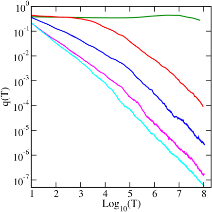
Figure 5: (Color online) Fluctuation index $q$ for fixed the energy density $h=1$ with $R=12$. From top to bottom: $E_{J}=0.1$ (green), $E_{J}=0.5$ (red), $E_{J}=1.0$ (blue), $E_{J}=2.0$ (magenta) and $E_{J}=3.0$ (cyan).

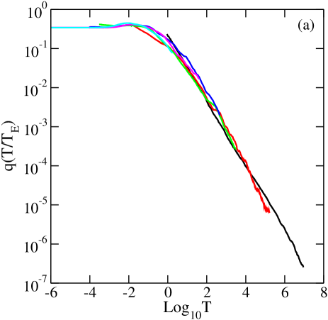
Figure 6: (Color online) a) $q(T/T_{E})$ for fixed $E_{J}=1$ with energy densities 0.1 (black) 1.2 (red), 2.4 (green), 3.8 (blue), 5.4 (magenta), and 8.5 (cyan) (corresponding to Fig. 1 in the main body); b) $q(T/T_{E})$ for fixed energy density $h=1$ with $E_{J}=0.5$, (red), $E_{J}=1.0$, (blue), $E_{J}=2.0$, (magenta) and $E_{J}=3.0$, (cyan) (corresponding to Fig. 5).

V Finite time average for $h=1$

Fig. 5 shows the index $q(T)$ for fixed energy $h=1$ with varying coupling strengths, $E_{J}$. It is similar to Fig.1 from the main text for fixed $E_{J}$ and varying $h$.

VI Evaluation of the ergodization time

We rescale and fit the fluctuation index $q(T)$ shown in Figs. 1 (main body) and 5 (in the supplement). We choose a parameter set with a clearly observed asymptotic $q(T)\approx T_{E}/T$ dependence, and fit this dependence to obtain $T_{E}$. We then rescale the variable $T\rightarrow xT$ for all other lines to obtain the best overlap with the initially chosen line as shown in Fig. 6. The scaling parameters $x$ are then used to compute the corresponding ergodization times.

VII Estimate of the ergodization time $T_{E}$

In the main text, we defined the ergodization time $T_{E}$ as the prefactor of the $1/T$ decay of the fluctuation index: $q(T\ll T_{E})=q(0)$ and $q(T\gg T_{E})\sim T_{E}/T$. We estimate this prefactor by approximating the time-dynamics of the observables $k_{n}(t)$ with telegraphic random process Richard (1972); Chakravarty and Kivelson (1985); Kac et al. (1963).

$$k_{n}(t)\approx\left\{\begin{array}[]{ll}k+\alpha\qquad\text{if}&k_{n}(t)>k\\ k-\beta\qquad\text{if}&k_{n}(t)<k\end{array}\right.$$ (24)

with real constant $\alpha,\beta$ (for example see Fig. 4(a) of the main text, where $\alpha=1-k$ and $\beta=k$). This recast the finite time average $\overline{k}_{n,T}=\frac{1}{T}\int_{0}^{T}k_{n}(t)dt$ of $k_{n}$ to

$$\begin{split}\overline{k}_{n,T}&\approx\frac{k+\alpha}{T}\sum_{i=1}^{M_{n}^{+}}\tau_{n}^{+}(i)+\frac{k-\beta}{T}\sum_{i=1}^{M_{n}^{-}}\tau_{n}^{-}(i)\\ &\equiv k+\frac{1}{T}\left[\alpha S_{n}^{+}-\beta S_{n}^{-}\right]\end{split}$$ (25)

since $T=S_{n}^{+}+S_{n}^{-}$. Here $M_{n}^{\pm}$ denote the number of excursions $\tau^{\pm}$ within a time interval $[0,T]$. As $\mu_{k}(T\rightarrow\infty)=k$ and $\sigma_{k}(T\rightarrow\infty)=0$ (see main text), we focus only on the variance $\sigma_{k}(T)$ to estimate the dependence on $T$ of the fluctuation index $q(T)=\frac{\sigma_{k}^{2}(T)}{\mu_{k}^{2}(T)}$. We first rewrite Eq.(25) in terms of $S_{n}^{+}$ only by adding and subtracting $\beta S_{n}^{+}/T$

$$\begin{split}\overline{k}_{n,T}&\approx\frac{\alpha+\beta}{T}S_{n}^{+}+k-\beta\end{split}$$ (26)

By recalling that $\sigma_{k+B}^{2}(T)=\sigma_{k}^{2}(T)$ and $\sigma_{Bk}^{2}(T)=B^{2}\sigma_{k}^{2}(T)$ for any constant $B$, and by dropping the constant factor $(\alpha+\beta)$ it follows that $\sigma_{k}^{2}(T)$ scales as

$$\sigma_{k}^{2}(T)\sim\frac{1}{T^{2}}\sigma_{S_{n}^{+}}^{2}(T)$$ (27)

As the excursion times $\tau^{+}$ are considered independent variables identically distributed, it follows that

$$\sigma_{S_{n}^{+}}^{2}(T)=M_{n}^{+}(T)\sigma_{\tau}^{2}$$ (28)

with $\sigma_{\tau}^{2}$ the variance of $\tau^{+}$. For $T\gg\mu_{\tau}$ with $\mu_{\tau}$ the first moment of $\tau^{+}$, the number of events $M_{n}^{+}$ grows as $M_{n}^{+}\sim T/\mu_{\tau}$. This yields

$$\sigma_{k}^{2}(T)\sim\frac{\sigma^{2}_{\tau}}{\mu_{\tau}}\frac{1}{T}$$ (29)

and ultimately to Eq. (4) of the main text.

VIII Lyapunov exponent computation

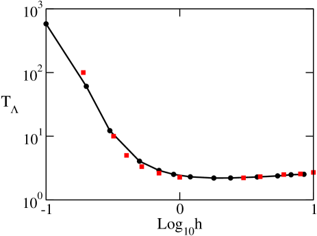
Figure 7: (Color online) Lyapunov time for fixed $E_{J}=1$. The black circles represent our numerical results, and the red squares represent the analytical results from Casetti et al. (1996). The black line guides the eye.

We compute the largest Lyapunov exponent $\Lambda$ by numerically solving the variational equations

$$\dot{w}(t)=\big{[}J_{2N}\cdot D_{H}^{2}(x(t))\big{]}\cdot w(t)$$ (30)

for a small amplitude deviation $w(t)=(\gamma q(t),\gamma p(t))$ coordinates. The largest Lyapunov exponent $\Lambda$ follows

$$\Lambda=\lim_{t\rightarrow\infty}\frac{1}{t}\ln\frac{\|w(t)\|}{\|w(0)\|}.$$ (31)

In Fig. 7 we show the Lyapunov time $T_{\Lambda}=1/\Lambda$ versus energy densities $h$ for given $E_{J}=1$. It matches well with the analytical results obtained in Casetti et al. (1996).

References

- Lichtenberg and Lieberman (1992) A. J. Lichtenberg and M. A. Lieberman, “Regular and Chaotic Dynamics, vol. 38 of,” Applied Mathematical Sciences (1992).
- Gaveau and Schulman (2015) B. Gaveau and L. S. Schulman, “Is ergodicity a reasonable hypothesis for macroscopic systems?” The European Physical Journal Special Topics 224, 891 (2015).
- Biroli and Tarzia (2017) G. Biroli and M. Tarzia, “Delocalized glassy dynamics and many-body localization,” Phys. Rev. B 96, 201114 (2017).
- Pérez-Espigares et al. (2018) C. Pérez-Espigares, F. Carollo, J. P. Garrahan, and P. I. Hurtado, “Dynamical criticality in driven systems: non-perturbative results, microscopic origin and direct observation,” arXiv preprint arXiv:1807.10235 (2018).
- Tong and Tanaka (2018) H. Tong and H. Tanaka, “Revealing Hidden Structural Order Controlling Both Fast and Slow Glassy Dynamics in Supercooled Liquids,” Phys. Rev. X 8, 011041 (2018).
- Senanian and Narayan (2018) A. Senanian and O. Narayan, “Glassy dynamics in disordered oscillator chains,” Phys. Rev. E 97, 062110 (2018).
- Bouchaud (1992) J.-P. Bouchaud, “Weak ergodicity breaking and aging in disordered systems,” Journal de Physique I 2, 1705 (1992).
- Bel and Barkai (2005) G. Bel and E. Barkai, “Weak ergodicity breaking in the continuous-time random walk,” Physical Review Letters 94, 240602 (2005).
- Bel, G. and Barkai, E. (2006) Bel, G. and Barkai, E., “Weak ergodicity breaking with deterministic dynamics,” Europhys. Lett. 74, 15 (2006).
- Rebenshtok and Barkai (2007) A. Rebenshtok and E. Barkai, “Distribution of Time-Averaged Observables for Weak Ergodicity Breaking,” Phys. Rev. Lett. 99, 210601 (2007).
- Rebenshtok and Barkai (2008) A. Rebenshtok and E. Barkai, “Weakly Non-Ergodic Statistical Physics,” J. Stat. Phys. 133, 565 (2008).
- Korabel and Barkai (2009) N. Korabel and E. Barkai, “Pesin-Type Identity for Intermittent Dynamics with a Zero Lyapunov Exponent,” Phys. Rev. Lett. 102, 050601 (2009).
- Schulz and Barkai (2015) J. H. P. Schulz and E. Barkai, “Fluctuations around equilibrium laws in ergodic continuous-time random walks,” Phys. Rev. E 91, 062129 (2015).
- Cataliotti et al. (2001) F. S. Cataliotti, S. Burger, C. Fort, P. Maddaloni, F. Minardi, A. Trombettoni, A. Smerzi, and M. Inguscio, “Josephson Junction Arrays with Bose-Einstein Condensates,” Science 293, 843 (2001).
- Ryu et al. (2013) C. Ryu, P. W. Blackburn, A. A. Blinova, and M. G. Boshier, “Experimental Realization of Josephson junctions for an Atom SQUID,” Phys. Rev. Lett. 111, 205301 (2013).
- Cassidy et al. (2017) M. C. Cassidy, A. Bruno, S. Rubbert, M. Irfan, J. Kammhuber, R. N. Schouten, A. R. Akhmerov, and L. P. Kouwenhoven, “Demonstration of an ac Josephson junction laser,” Science 355, 939 (2017).
- Blackburn et al. (2016) J. A. Blackburn, M. Cirillo, and N. Grønbech-Jensen, “A survey of classical and quantum interpretations of experiments on Josephson junctions at very low temperatures,” Physics Reports 611, 1 (2016).
- Tsygankov and Wiesenfeld (2002) D. Tsygankov and K. Wiesenfeld, “Spontaneous synchronization in a Josephson transmission line,” Phys. Rev. E 66, 036215 (2002).
- El-Nashar et al. (2003) H. F. El-Nashar, Y. Zhang, H. A. Cerdeira, and F. Ibiyinka A., “Synchronization in a chain of nearest neighbors coupled oscillators with fixed ends,” Chaos: An Interdisciplinary Journal of Nonlinear Science 13, 1216 (2003).
- Binder et al. (2000) P. Binder, D. Abraimov, A. V. Ustinov, S. Flach, and Y. Zolotaryuk, “Observation of breathers in Josephson ladders,” Phys. Rev. Lett. 84, 745 (2000).
- Miroshnichenko et al. (2001) A. E. Miroshnichenko, S. Flach, M. V. Fistul, Y. Zolotaryuk, and J. B. Page, “Breathers in Josephson junction ladders: Resonances and electromagnetic wave spectroscopy,” Phys. Rev. E 64, 066601 (2001).
- Fistul et al. (2002) M. V. Fistul, A. E. Miroshnichenko, S. Flach, M. Schuster, and A. V. Ustinov, “Incommensurate dynamics of resonant breathers in Josephson junction ladders,” Phys. Rev. B 65, 174524 (2002).
- Miroshnichenko et al. (2005) A. E. Miroshnichenko, M. Schuster, S. Flach, M. V. Fistul, and A. V. Ustinov, “Resonant plasmon scattering by discrete breathers in Josephson junction ladders,” Phys. Rev. B 71, 174306 (2005).
- Shulga et al. (2018) K. V. Shulga, E. Il’ichev, M. V. Fistul, I. S. Besedin, S. Butz, O. V. Astafiev, U. Hübner, and A. V. Ustinov, “Magnetically induced transparency of a quantum metamaterial composed of twin flux qubits,” Nature Communications 9, 150 (2018).
- Martinis (2004) J. M. Martinis, “Course 13 - Superconducting Qubits and the Physics of Josephson Junctions,” in Quantum Entanglement and Information Processing, Les Houches, Vol. 79, edited by D. Estéve, J.-M. Raimond, and J. Dalibard (Elsevier, 2004) pp. 487 – 520.
- Gendelman and Savin (2000) O. V. Gendelman and A. V. Savin, “Normal Heat Conductivity of the One-Dimensional Lattice with Periodic Potential of Nearest-Neighbor Interaction,” Phys. Rev. Lett. 84, 2381 (2000).
- Giardinà et al. (2000) C. Giardinà, R. Livi, A. Politi, and M. Vassalli, “Finite Thermal Conductivity in 1D Lattices,” Phys. Rev. Lett. 84, 2144 (2000).
- Pino et al. (2016) M. Pino, L. B. Ioffe, and B. L. Altshuler, “Nonergodic metallic and insulating phases of Josephson junction chains,” PNAS 113, 536 (2016).
- Basko et al. (2006) D. Basko, I. Aleiner, and B. Altshuler, “Metal insulator transition in a weakly interacting many-electron system with localized single-particle states,” Annals of Physics 321, 1126 (2006).
- Escande et al. (1994) D. Escande, H. Kantz, R. Livi, and S. Ruffo, “Self-consistent check of the validity of Gibbs calculus using dynamical variables,” Journal of Statistical Physics 76, 605 (1994).
- De Roeck and Huveneers (2014) W. De Roeck and F. Huveneers, “Asymptotic Localization of Energy in Nondisordered Oscillator Chains,” Communications on Pure and Applied Mathematics 68, 1532 (2014).
- Mithun et al. (2018) T. Mithun, Y. Kati, C. Danieli, and S. Flach, “Weakly Nonergodic Dynamics in the Gross-Pitaevskii Lattice,” Phys. Rev. Lett. 120, 184101 (2018).
- Danieli et al. (2017) C. Danieli, D. K. Campbell, and S. Flach, “Intermittent many-body dynamics at equilibrium,” Phys. Rev. E 95, 060202 (2017).
- Casetti et al. (1996) L. Casetti, C. Clementi, and M. Pettini, “Riemannian theory of Hamiltonian chaos and Lyapunov exponents,” Phys. Rev. E 54, 5969 (1996).
- Casetti et al. (2000) L. Casetti, M. Pettini, and E. Cohen, “Geometric approach to Hamiltonian dynamics and statistical mechanics,” Physics Reports 337, 237 (2000).
- Livi et al. (1987) R. Livi, M. Pettini, S. Ruffo, and A. Vulpiani, “Chaotic behavior in nonlinear Hamiltonian systems and equilibrium statistical mechanics,” Journal of Statistical Physics 48, 539 (1987).
- (37) See Supplemental Material at [URL will be inserted by publisher] for additional information, which include Refs.Skokos et al. (2009); Richard (1972); Chakravarty and Kivelson (1985); Kac et al. (1963) .
- Chirikov (1979) B. V. Chirikov, “A universal instability of many-dimensional oscillator systems,” Physics Reports 52, 263 (1979).
- Kolmogorov (1954) A. N. Kolmogorov, “On conservation of conditionally periodic motions for a small change in Hamilton’s function,” Dokl. Akad. Nauk SSSR 98, 527 (1954).
- Arnold (1963) V. Arnold, “A proof of a theorem by a.n. kolmogorov on the invariance of quasi-periodic motions under small perturbations of the hamiltonian,” Russ. Math. Surv. 18, 9 (1963).
- Moser (1962) J. Moser, “On invariant curves of area-preserving mappings of an annulus,” Nachr. Akad. Wiss. Gottingen, II , 1 (1962).
- Chierchia and Gallavotti (1982) L. Chierchia and G. Gallavotti, “Smooth prime integrals for quasi-integrable hamiltonian systems,” Il Nuovo Cimento B 67, 277 (1982).
- Benettin et al. (1984) G. Benettin, L. Galgani, A. Giorgilli, and J. M. Strelcyn, “A proof of kolmogorov’s theorem on invariant tori using canonical transformations defined by the lie method,” Il Nuovo Cimento B 79, 201 (1984).
- Wayne (1984a) C. E. Wayne, “The kam theory of systems with short range interactions, 1,” Comm. Math. Phys. 96, 311 (1984a).
- Wayne (1984b) C. E. Wayne, “The kam theory of systems with short range interactions, 2,” Comm. Math. Phys. 96, 331 (1984b).
- Skokos et al. (2009) C. Skokos, D. O. Krimer, S. Komineas, and S. Flach, “Delocalization of wave packets in disordered nonlinear chains,” Phys. Rev. E 79, 056211 (2009).
- Richard (1972) P. Richard, “Feynman. statistical Mechanics, a set of lectures,” Frontiers in Physics. Perseus Books (1972).
- Chakravarty and Kivelson (1985) S. Chakravarty and S. Kivelson, “Photoinduced macroscopic quantum tunneling,” Phys. Rev. B 32, 76 (1985).
- Kac et al. (1963) M. Kac, G. Uhlenbeck, and P. Hemmer, “On the van der Waals Theory of the Vapor-Liquid Equilibrium. i. Discussion of a One-Dimensional Model,” Journal of Mathematical Physics 4, 216 (1963).