Bayesian Nonparametric Policy Search with Application to Periodontal Recall Intervals

Abstract

Tooth loss from periodontal disease is a major public health burden in the United States. Standard clinical practice is to recommend a dental visit every six months; however, this practice is not evidence-based, and poor dental outcomes and increasing dental insurance premiums indicate room for improvement. We consider a tailored approach that recommends recall time based on patient characteristics and medical history to minimize disease progression without increasing resource expenditures. We formalize this method as a dynamic treatment regime which comprises a sequence of decisions, one per stage of intervention, that follow a decision rule which maps current patient information to a recommendation for their next visit time. The dynamics of periodontal health, visit frequency, and patient compliance are complex, yet the estimated optimal regime must be interpretable to domain experts if it is to be integrated into clinical practice. We combine non-parametric Bayesian dynamics modeling with policy-search algorithms to estimate the optimal dynamic treatment regime within an interpretable class of regimes. Both simulation experiments and application to a rich database of electronic dental records from the HealthPartners HMO shows that our proposed method leads to better dental health without increasing the average recommended recall time relative to competing methods.

Key words: Dirichlet process prior; dynamic treatment regimes; observational data; periodontal disease; practice-based setting; precision medicine; sequential optimization

1 Introduction

Periodontal disease (PD) contributes to eventual tooth loss and remains a major health burden. The ultimate goal of professional periodontal maintenance plans (AAP, 2001) and personal oral care is PD prevention and maintaining teeth in a state of comfort and function. The total dental healthcare spending in the United States in 2013 was a staggering US$ 91.8 billion (Wall, Thomas and Guay, Albert, 2016), and is continually increasing (CDC, 2010). Hence, there is an urgent need to reduce cost without diminishing the quality of care. In the context of dental care, updating periodontal recall recommendations to reflect the individual needs of each patient holds the potential to both improve oral health and reduce cost. The length of periodontal recall intervals has been a topic of research and debate for decades (Lövdal et al., 1961; Axelsson et al., 1991; Fardal et al., 2004; Mettes, 2005; Riley et al., 2013) with recommendations for recall intervals ranging from two weeks (Nyman et al., 1975) to eighteen months (Rosén et al., 1999). The current standard of care, which was advocated as early as 1879 by the American Academy of Dental Science (Teich, 2013), is a recall interval of six months for all patients regardless of individual demographics, oral health, family history, or other risk factors. Existing clinical guidelines recommend that the recall intervals should depend on individual patient characteristics (NCCAC, 2004; Patel et al., 2010; see also Giannobile et al., 2013) but offer little concrete guidance on how to map individual patient characteristics to a recall interval.

The potential effect of altering such intervals on oral health had remained the subject of international debate for almost 3 decades (Mettes, 2005; Riley et al., 2013). Infrequent dental visits might impair the ability to diagnose PD at an early stage, present fewer opportunities for providing oral-care education, and block the opportunities for effective treatments (Davenport et al., 2003). However, unnecessary visits and treatments waste the resources and increase the cost. Therefore, the recall interval should be tailored to individual needs. Patients at high risk may benefit from more frequent visits while less frequent visits might be adequate for subjects without certain risk factors of PD (Giannobile et al., 2013). This provides evidence that a personalized (or precision) medicine approach (Kornman and Duff, 2012; Zanardi et al., 2012) might improve resource allocation for preventive dentistry.

In this paper, we consider adaptive recall intervals that recommend a recall time for each patient at each visit depending on their personal characteristics, including disease history. We formalize a personalized recall interval policy as a function that maps current patient information to a recommended recall interval, which is an example of a dynamic treatment regime, or DTR (Murphy, 2003; Robins, 2004; Chakraborty and Moodie, 2013; Schulte et al., 2014; Kosorok and Moodie, 2015). A DTR is defined as a sequence of decision rules, one per stage of intervention, to make treatment decisions based on the patient’s evolving status. Each decision rule takes the individual’s information up to that time point as the input, and outputs a recommended treatment at that stage. The optimal DTR is defined as the regime that optimizes the mean long-term outcome. The problem we are addressing is to specify a regime that uses a patient’s up-to-date information to tailor recall interval recommendations in such a way that maximizes long-term population-level benefits, and it is thus a DTR problem. DTRs have been applied across a wide range of application domains to estimate data-driven intervention policies (van der Laan and Petersen, 2007; Robins et al., 2008; Shortreed and Moodie, 2012; Laber et al., 2014; Almirall et al., 2014; Wu et al., 2015); however, estimation of an optimal recall intervention policy presents several challenges that make existing estimation methods unsuitable without modification. These challenges include: (i) cost constraints on recall frequency across the entire population; (ii) non-compliance and sparse irregularly spaced clinic visits; (iii) a bounded response with a large point mass on the response of the previous time point due to clinicians carrying forward previous measurements rather than retaking them; and (iv) the requirement that the estimated policy be clinically interpretable, despite complex disease dynamics. Existing methods for cost-constrained DTRs include cost-constrained IQ-learning (Linn et al., 2016) which only applies for two decision points; cost-sensitive DTRs (Luedtke and van der Laan, 2016) which constrain the proportion of individuals who can receive treatment; set-valued DTRs (Laber et al., 2014; Lizotte and Laber, 2016) which allow for multivariate outcomes, e.g., cost and efficacy, but do not permit constrained estimation. Functional and longitudinal methods for DTRs can accommodate sparse and irregularly-spaced observation times (Ciarleglio et al., 2015; Lu et al., 2016; Laber and Staicu, 2016), however, these methods are not designed for application with many, possibly outcome-driven, follow-up times, nor can they deal with non-compliance.

Policy-search is a common method for estimation of a DTR, and is particularly well-suited to constrained problems (Chakraborty and Moodie, 2013; Wang et al., 2018; Laber et al., 2018). Policy-search methods postulate a model for the marginal mean outcome under each policy within a pre-specified class of policies and choose the maximizer as the estimated optimal policy (Robins et al., 2008; Orellana et al., 2010; Zhang et al., 012a; Zhang et al., 012b; Zhao et al., 2012; Zhang et al., 2013; Zhao et al., 2015; Kosorok and Moodie, 2015; Guan et al., 2016; Zhou and Kosorok, 2017). An advantage of policy-search methods is that models for the underlying disease progression can be decoupled from the class of policies, thereby allowing for complex disease models with parsimonious, interpretable, or cost-constrained estimated optimal policies (Zhang et al., 2015; Laber and Zhao, 2015; Lakkaraju and Rudin, 2016). However, existing methods for policy-search are difficult to implement for complex data structures, like the one we consider here.

We use a Bayesian nonparametric (BNP) disease dynamics model and g-computation (Robins, 1986) to construct an estimator of the marginal mean outcome and cost under any policy within a pre-specified class, and then use stochastic optimization to approximate the maximizer of the mean outcome under a constraint on cost. The marginal mean outcome is cumulative, and accounts for disease progression and delayed effects of treatment. We estimate this marginal mean outcome using g-computation, which accounts for these effects and other time-varying causal confounding. The proposed dynamics model is sufficiently flexible to accommodate non-compliance, sparse and irregularly-spaced visits; however, our class of policies is based on a clinically interpretable risk score. BNP methods have recently been used in the context of estimating optimal treatment regimes (Arjas and Saarela, 2010; Xu et al., 2016; Murray et al., 2017), but they did not consider regimes that adapt to the evolving health status of each individual patient, or cost constraints.

The motivation for establishing this (recall) recommendation engine comes from analyzing an observational database in a dental practice-based setting, collected by the HealthPartners®(HP) Institute at Minneapolis, Minnesota. In Section 2, we review the HP data. In Section 3, we formalize the recall estimation problem using a decision theoretic framework. In Section 4, we present a BNP formulation of the disease dynamics and in Section 5, we combine this model with a stochastic optimization algorithm to construct an estimator of the optimal intervention policy subject to constraints on cost. In Section 6, we evaluate the finite sample performance of the proposed methods using a suite of simulation experiments. We analyze the motivating HP dataset and summarize the fitted policy in Section 7. Finally, we conclude with a brief discussion in Section 8.

2 HealthPartners Data

The motivating longitudinal HP dataset were collected from routine dental practice in the Minneapolis area. We include only adult subjects with at least two visits, giving 24,731 subjects with as many as 8 years of irregular longtitudinal follow-up, with an average of 8.6 visits. For each subject, we use the data from the first visit until the last visit to fit the model proposed in Section 3, and so the follow-up window varies by subject. During each visit, periodontal pocket depth (PPD) is recorded at six pre-specified sites per tooth (excluding the third molars) giving 168 measurements for a full mouth without any missing tooth. In concordance with the proposed standards from the joint EU/USA Periodontal Working Group (Holtfreter et al., 2015), we use the proportion of diseased/affected tooth sites (with PPD $>$ 3mm, or missing tooth) per mouth, henceforth PMU, as our response to measure the extent (severity) of PD. Note, when the tooth is missing, we assume the missing is due to PD and we classify all sites associated with the missing tooth are diseased tooth sites. So each missing tooth contributes to 6 diseased tooth sites in the calculation. Demographic information and medical history are also collected, including age (ranging from 19 to 97 years, with mean 55 years), gender (49% male, 51% female), race (85% white, 15% non white), diabetes status (8% with diabetes, 92% without diabetes), smoking status (9% current tobacco user, 91% not current user), and insurance information (80% with commercial insurance, 20% without commercial insurance).

Figure 1 plots the longitudinal profiles for 10 subjects. Although there are some short-term decreases, there is a clear population-level increasing trend. A high proportion of the responses are identical to the previous response, reflecting the common practice of carrying the previous values forward in the dental record if there is no apparent change in disease status. During each visit, the recommended time until the next visit ($A$) is also recorded, and the actual time between two visits ($\delta$) is computed. HP uses an algorithm to classify subjects as low, medium or high risk of PD and caries, and this risk score is taken into consideration when recommending the next visit time. However, this risk score is not optimized for recall recommendations, and dentists are not obliged to use it. The range of $A$, as indicated in Figure 2, varies significantly from 3 months to 18 months. The figure also illustrates the partial controllability, with a strong but imperfect relationship between observed and recommended recall times ($A$) between visits.

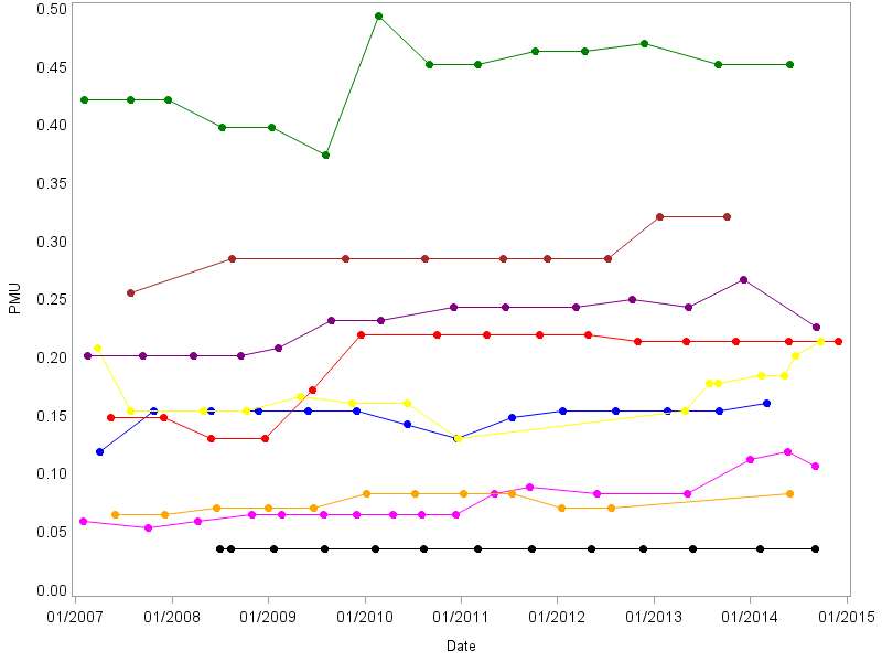
Figure 1: The proportion of sites with unhealthy PPD (pocket depth exceeding 3mm) or missing tooth, denoted by PMU, over time, for 10 randomly chosen subjects.

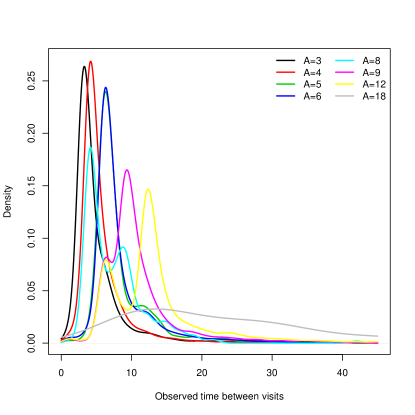
Figure 2: Density plots of actual time between visits ($\delta$ months) for each level of recommended recall interval ($A$ months).

3 Problem statement

The data at baseline for subject $i=1,\ldots,n$ include the $p$-vector of covariates, $\mbox{\bf X}_{i}$ and the scalar baseline response, $Y_{i0}$. At the baseline visit, a recommended number of months until the first follow-up visit $A_{i1}(>0)$ is given. The subject returns for the first following visit $\delta_{i1}(>0)$ months after the baseline visit, and the subject’s response, $Y_{i1}$, is recorded. This process is repeated for $N_{i}$ follow-up visits for the subject $i$. The data available after visit $t$ for subject $i$ are $\mbox{\bf H}_{it}=\{\mbox{\bf X}_{i},Y_{i0},A_{i1},\delta_{i1},Y_{i1},\ldots,A_{it_{i}},\delta_{it},Y_{it}\}$, and $\mbox{\bf H}_{i}\equiv\mbox{\bf H}_{iN_{i}}$ is the entire history for subject $i$. The subscript $i$ is suppressed to denote a generic trajectory $\mbox{\bf H}_{t}=\{\mbox{\bf X},Y_{0},A_{1},\delta_{1},Y_{1},\ldots,A_{t},\delta_{t},Y_{t}\}$.

Our objective is to use these data to determine a policy for recommending the time between visits. A policy $\pi$ is a deterministic function that maps the available data to a recommendation, i.e., under $\pi$,

$$A_{t}=\pi(\mbox{\bf H}_{t};\mbox{\boldmath$\alpha$}).$$ (1)

The policy is parameterized in terms of the unknown vector $\mbox{\boldmath$\alpha$}=(\alpha_{1},\ldots,\alpha_{q})^{T}$. For interpretability, we assume that the policy is a function of a risk score that is a linear combination of features constructed from $\mbox{\bf H}_{t}$, $\mbox{\bf f}(\mbox{\bf H}_{t})=[f_{1}(\mbox{\bf H}_{t}),\ldots,f_{q}(\mbox{\bf H}_{t})]^{T}$. There is great flexibility in constructing the features; they can include the covariates themselves, $f_{k}(\mbox{\bf H}_{t})=X_{j}$, or composites such as change from baseline $f_{k}(\mbox{\bf H}_{t})=Y_{t}-Y_{0}$, or even summaries of the posterior predictive distribution. The risk score is then $R_{t}=\mbox{\bf f}(\mbox{\bf H}_{t})^{T}\mbox{\boldmath$\alpha$}$, and subjects with high risk scores are recommended to have small $A_{t}$, whereas subjects with low risk are recommended to a larger $A_{t}$. While including many features can give a rich class of policies, we consider a small value of $q$ so that the subclass of policies is interpretable, and the optimization problem reduces to estimating the low-dimensional vector $\alpha$. We use $\Pi$ to denote the above pre-specified class of policies that are parameterized by $\alpha$.

We formalize the optimal recall interval recommendation policy within the class $\Pi$ using potential outcomes. Define $Y_{t}^{\star}(\overline{a}_{t})$ and $\delta_{t}^{\star}(\overline{a}_{t})$ to be the potential PMU outcome at visit $t$ and potential time between visit $t$ and visit $t-1$, respectively, if the sequence of recall recommendations $\overline{a}_{t}$ would be given to a subject since baseline visit, where $\overline{a}_{t}=\{a_{1},\dots,a_{t}\}$ denotes the history of recall interval recommendations up to visit $t$ . Define $Y_{t}^{\star}(\pi)$, $\delta_{t}^{\star}(\pi)$ to be the potential outcomes at visit $t$ under recall interval recommendation policy $\pi$. The value associated with a policy can be defined as the expectation of a function of potential outcomes under the policy, e.g., $V(\pi)=\mathbb{E}\{[1/J^{\star}(\pi)]\sum_{t=1}^{J^{\star}(\pi)}Y_{t}^{\star}(\pi)\}$, where $J^{\star}(\pi)$ is the number of visits within a pre-specified time period under policy $\pi$. The optimal policy within the pre-specified class of policies is $\pi_{opt}=\underset{\pi\in\Pi}{\arg\max}\ V(\pi)$. In order to estimate the optimal recall interval recommendation policy within the pre-specified class using the observed data, we make the following assumptions: (1) no unmeasured confounders (or sequential ignorability) (Robins, 2004), $\{(Y_{k}^{\star}(\overline{a}_{k}),\delta_{k}^{\star}(\overline{a}_{k})):\text{ for all }\overline{a}_{k}\in\overline{\mathscr{A}_{k}}\}_{k\geq 1}\perp\!\!\!\perp A_{t}|\mbox{\bf H}_{t}$ for $t=1,\dots,N$, where $\overline{\mathscr{A}_{k}}=\mathscr{A}_{1}\times\dots\times\mathscr{A}_{k}$ is the set of all possible recall interval recommendations up to visit $k$; (2) consistency, $Y_{t}=Y^{\star}(\overline{A}_{t})$ and $\delta_{t}=\delta^{\star}(\overline{A}_{t})$, where $\overline{A}_{t}$ is the sequence of observed recommended recall intervals up to visit $t$, i.e., the observed outcomes are the potential outcomes under the actual given recall interval recommendation; (3) positivity, there exists $\epsilon>0$ so that $P(A_{t}=a_{t}|\mbox{\bf H}_{t}=h_{t})\geq\epsilon$ for all $a_{t}\in\Psi_{t}(h_{t})$ and for all $h_{t}$, where $\Psi_{t}(h_{t})$ is the set of possible recall interval recommendations for a subject with realized history information $h_{t}$, $t=1,\dots,N$. Under those assumptions, our framework of estimating optimal policy is causally interpretable (Robins, 2004; Schulte et al., 2014), and we use the notation of the generic trajectory instead of potential outcomes hereafter.

To compare policies, we use a utility function $U(\mbox{\bf H})$, which is considered the primary outcome to be optimized. Based on the underlying clinical science and logistical constraints, we chose 5-year mean reduction in the proportion of unhealthy sites as one of our primary outcomes; however, the proposed methodology can be extended to other time horizons, or other summaries of a patient’s health trajectory. We desire a policy that applies to all subjects, and we therefore compare the population mean utility, called the value, $V(\mbox{\boldmath$\alpha$})=\mathbb{E}_{\mbox{\boldmath$\alpha$}}[U(\mbox{\bf H})]$. The expectation averages over the entire distribution of H, including the baseline covariates, the visit times as determined by $\delta_{t}$, and the PMU trajectory $Y_{0},\ldots,Y_{N}$. The policy vector $\alpha$ alters the value indirectly via the recommendation times $A_{t}$ which subsequently affect the time courses of $\delta_{t}$ and dental health state $Y_{t}$. Therefore, estimating the value of the policy requires determining compliance relationship (the distribution of $\delta_{t}$ given $A_{t}$), and the effect of recall on PD (the distribution of $Y_{t}$ given $\delta_{t}$). In addition to value, policies must be compared in terms of their cost because it is not feasible to recommend a short time between visits for all subjects. We control cost by constraining the average recommended recall time to be $T$, $C(\mbox{\boldmath$\alpha$})=\mathbb{E}_{\mbox{\boldmath$\alpha$}}(A_{t})=T$.

The objective is to identify an $\alpha$ which maximizes the value $V(\mbox{\boldmath$\alpha$})$ while maintaining cost constraint $C(\mbox{\boldmath$\alpha$})=T$. Rather than attempting to estimate $\alpha$ directly from the data, our approach is to first estimate the distribution of H as a function of $\alpha$ using a BNP model (Section 4). Given this model, we can then simulate from the process to obtain Monte Carlo estimates of $V(\mbox{\boldmath$\alpha$})$ and $C(\mbox{\boldmath$\alpha$})$ for any $\alpha$, and use this simulation as a basis for determining the optimal $\alpha$ (Section 5).

4 Bayesian model for disease progression

For our application, we build a Dirichlet Process Mixture (DPM) model that is parsimonious enough to fit large data sets and facilitate the extensive simulation required for policy evaluation, yet flexible enough to capture the complex dynamics of the HP data. Heterogeneity across subjects is captured with subject random effects $\Theta_{i}=\{\mbox{\boldmath$\theta$}_{i0},\mbox{\boldmath$\theta$}_{i1},\mbox{\boldmath$\theta$}_{i2}\}$ that includes random effects for baseline status ($\mbox{\boldmath$\theta$}_{i0}$), compliance ($\mbox{\boldmath$\theta$}_{i1}$), and disease progression ($\mbox{\boldmath$\theta$}_{i2}$), and is modeled using Bayesian nonparametrics as described below. Given the random effects, we propose a Markov outcome-dependent follow-up model (Ryu et al., 2007) for $\mbox{\bf H}_{i}$,

$$(\mbox{\bf X}_{i}^{T},Y_{i0})^{T}|\Theta_{i} \sim \mbox{Normal}(\mbox{\boldmath$\theta$}_{i0},\mbox{\boldmath$\Sigma$}_{0})$$ (2)

$$\log(\delta_{it})|\Theta_{i},\mbox{\bf X}_{i},Y_{it-1},A_{it} \sim \mbox{Normal}({\cal X}_{it}^{T}\mbox{\boldmath$\theta$}_{i1},\sigma_{1}^{2})$$

$$Y_{it}|\Theta_{i},\mbox{\bf X}_{i},Y_{it-1},\delta_{it} \sim \mbox{Normal}({\cal Z}_{it}^{T}\mbox{\boldmath$\theta$}_{i2},\sigma_{2}^{2})$$

where ${\cal X}_{it}=[\mbox{\bf X}_{i}^{T},Y_{it-1},\log(A_{it}),\mbox{\bf X}_{i}^{T}\log(A_{it}),Y_{it-1}\log(A_{it})]^{T}$ and ${\cal Z}_{it}=(\mbox{\bf X}_{i}^{T},Y_{it-1},\delta_{it},\mbox{\bf X}_{i}^{T}\delta_{it},Y_{it-1}\delta_{it})^{T}$.

Although this first-stage model is relatively simple, the overall model is flexible when integrated over the random effects $\Theta_{i}$. For example, compliance $\delta_{it}/A_{it}$ depends on both covariates and current disease status, and these relationships are individualized through $\mbox{\boldmath$\theta$}_{i1}$. Similarly, the individualized treatment effect is controlled by $\mbox{\boldmath$\theta$}_{i2}$ and the induced relationship between $\delta_{it}$, $Y_{it-1}$, and $Y_{it}$. Also, prior correlation between $\mbox{\boldmath$\theta$}_{i0}$ and $\mbox{\boldmath$\theta$}_{i2}$ can accommodate effect modification between the baseline covariates and time between visits in the PMU model. Of course, even more flexible models can be constructed using non-linear terms in ${\cal X}_{it}$ and ${\cal Z}_{it}$ and higher-order lags in the Markov model.

Let $g$ be the random effects density, such that $\Theta_{i}\stackrel{{\scriptstyle iid}}{{\sim}}g(\Theta)$. Rather than selecting a parametric model for $g$, we treat the density as an unknown quantity to be estimated from the data. The prior for $g$ is modeled using the Dirichlet process prior (Ferguson, 1973; Sethuraman, 1994), which can be written as $g(\Theta)=\sum_{l=1}^{L}\omega_{l}\mathbbm{1}_{\Delta_{l}}(\Theta)$, where $L=\infty$, the mixture probabilities $\omega_{l}>0$ satisfy $\sum_{l=1}^{\infty}\omega_{l}=1$, $\Delta_{l}=(\mbox{\boldmath$\theta$}_{0l}^{\star T},\mbox{\boldmath$\theta$}^{\star T}_{1l},\mbox{\boldmath$\theta$}_{2l}^{\star T})^{T}\sim\text{Normal}(\bm{m}_{b},\mbox{\boldmath$\Sigma$}_{b})$, and $\mathbbm{1}_{\Delta_{l}}(\cdot)$ is the indicator function with a point mass at $\Delta_{l}$. The mixture probabilities can be generated from the stick-breaking process: $\omega_{l}=V_{l}\prod_{h<l}(1-V_{h})$, $V_{l}\sim\text{Beta}(1,\alpha_{0})$. The covariance matrix $\mbox{\boldmath$\Sigma$}_{b}$ is taken to be block diagonal with $\mbox{Cov}(\mbox{\boldmath$\theta$}_{jl}^{\star})=\mbox{\boldmath$\Sigma$}_{bj}$ and $\mbox{Cov}(\mbox{\boldmath$\theta$}_{jl}^{\star},\mbox{\boldmath$\theta$}_{kl}^{\star})=0$. For priors, we select $\bm{m}_{b}\sim\mbox{Normal}(0,I)$ and $\mbox{\boldmath$\Sigma$}_{bj}\sim\mbox{InvWishart}(p_{j}+1,(p_{j}+1)I_{p_{j}})$, where $p_{j}$ is the dimension of $\mbox{\boldmath$\theta$}^{\star}_{jl}$. With these priors and truncation at a finite $L$, all full conditional distributions are conjugate and so we use Gibbs sampling to obtain posterior samples as described in the supplemental material.

5 Policy search

Although other classes of policies are possible, such as trees (Laber and Zhao, 2015) and lists (Zhang et al., 2015), we consider policies defined by a linear risk score. Let the risk score be $R_{t}=\mbox{\bf f}(\mbox{\bf H}_{t})^{T}\mbox{\boldmath$\alpha$}$, where $\mbox{\bf f}(\mbox{\bf H}_{t})$ is a $q$-vector of features and $\mbox{\boldmath$\alpha$}=(\alpha_{1},\ldots,\alpha_{q})^{T}$ are their weights. Our general framework can easily accommodate non-linear relationships between patient characteristics and the risk score by including non-linear summaries of the characteristics as features. As an extreme example, we could include B-spline basis or tree expansion of a variable as features to give an arbitrarily flexible risk score. We could also include an interaction between a characteristic and disease status to account for different importance of the characteristic as the disease progresses. However, our goal is to develop a policy that is interpretable to domain experts so that it can be integrated to the clinical practice. Hence, we decided to keep the risk score simple. We describe the method assuming two possible recommendations, $a_{1}$ and $a_{2}$. The policy takes the form

$$A_{t}=\pi(\mbox{\bf H}_{t};\mbox{\boldmath$\alpha$})=\begin{cases}a_{1}&R_{t}>\kappa(\mbox{\boldmath$\alpha$})\\ a_{2}&R_{t}\leq\kappa(\mbox{\boldmath$\alpha$})\end{cases}$$ (3)

where $\kappa(\mbox{\boldmath$\alpha$})$ is the risk threshold that depends on $\alpha$; more than two treatments could be accommodated using multiple thresholds. With only a single threshold, the scale of $\alpha$ is irrelevant, and so we impose the restriction $||\mbox{\boldmath$\alpha$}||=(\sum_{j=1}^{q}\alpha_{j}^{2})^{1/2}=1$. Figure 3 illustrates how the proposed method is used when a sequence of recall intervals needs to be optimized under a given policy in terms of $\alpha$.

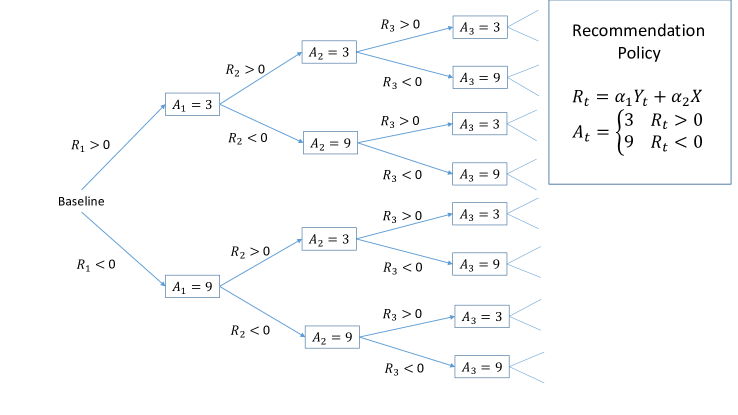
Figure 3: Illustration of how to optimize a sequence of recall intervals under a given policy using the proposed method. In this hypothetical example, the risk score $R_{t}$ is a linear combination of the current disease statue ($Y_{t}$) and a single covariate (X), and the two actions are to return in 3 or 9 months.

We select the policy parameters $\alpha$ so that when the population of patients follows this rule over time, the long-term average reward is high. Given the posterior of the random effects distribution $g$ and covariance parameters ${\cal S}=\{\Sigma,\sigma_{1},\sigma_{2}\}$, the optimal feature weight $\alpha$ is given by

$$\mbox{\boldmath$\alpha$}_{opt}=\underset{\mbox{\boldmath$\alpha$}}{\arg\max}\ V(\mbox{\boldmath$\alpha$})\mbox{\ \ such that \ \ }C(\mbox{\boldmath$\alpha$})=T.$$ (4)

However, this is a challenging optimization problem, because both $V(\mbox{\boldmath$\alpha$})$ and $C(\mbox{\boldmath$\alpha$})$ are expectations with respect to the predictive distribution of H given $g$ and ${\cal S}$. Both $V(\mbox{\boldmath$\alpha$})$ and $C(\mbox{\boldmath$\alpha$})$ are approximated using Monte Carlo sampling. The MCMC algorithm described in Section 4 produces $J$ posterior draws $\{g^{(j)},{\cal S}^{(j)};j=1,\ldots,J\}$. For each candidate $\alpha$ and $\kappa(\mbox{\boldmath$\alpha$})$, we simulate subject $i=1,\ldots,n_{0}$ by first sampling $j$ randomly from $\{1,\ldots,J\}$, then $\Theta_{i}\sim g^{(j)}$, and finally $\mbox{\bf H}_{i}$ from (2) given $\Theta_{i}$ and ${\cal S}^{(j)}$, with recommendations given by $\pi(\mbox{\bf H}_{it};\mbox{\boldmath$\alpha$})$. Note that in these simulations, the actions taken affect the future outcomes & thus future recommendtaions, and in this way the method can allow for delayed effects.

For each candidate $\alpha$, we first identify the threshold $\kappa(\mbox{\boldmath$\alpha$})$ that satisfies the cost constraint $C(\mbox{\boldmath$\alpha$})\approx T$, and then estimate the value $V(\mbox{\boldmath$\alpha$})$ given this threshold. We estimate $C(\mbox{\boldmath$\alpha$})$ separately for a grid of 10 thresholds spanning the range of $R_{t}$ in the training data, smooth the estimates using LOESS (Cleveland and Devlin, 1988), and then compute the $\kappa$ that gives $C(\mbox{\boldmath$\alpha$})\approx T$. For each of the 10 candidate thresholds, we draw $n_{1}=2,000$ independent subjects’ $\mbox{\bf H}_{i}$ and use the sample mean of the $n_{1}$ averaged recommended recall time as the estimate of $C(\mbox{\boldmath$\alpha$}$). Given the threshold $\kappa(\mbox{\boldmath$\alpha$})$, the value $V(\mbox{\boldmath$\alpha$})$ is approximated by another round of Monte Carlo simulation of $n_{2}=20,000$ subjects.

We utilize response-surface sequential optimization methodology (Mason et al., 2003) to identify the value of $\alpha$ that maximizes $V(\mbox{\boldmath$\alpha$})$. The objective function of this optimization is noisy because only a Monte Carlo estimate of the value is available. In the first stage, we evaluate the value using a central composite design for $\alpha$ (Montgomery, 2008), scaled to $||\mbox{\boldmath$\alpha$}||=1$. That is, we consider the $M_{1}=5^{q}-1$ unconstrained values ${\tilde{}\mbox{\boldmath$\alpha$}}\in\{-2,-1,0,1,2\}^{q}$ (excluding the zero vector), and then the corresponding constrained vectors $\mbox{\boldmath$\alpha$}_{l}=(\alpha_{l1},\ldots,\alpha_{lq})^{T}$ formed by setting $\alpha_{lj}=\tilde{\alpha}_{lj}/\sqrt{\sum_{h=1}^{q}{\tilde{\alpha}}_{lh}^{2}}$, such that $||\mbox{\boldmath$\alpha$}_{l}||=1$. A Monte Carlo estimate of the value ${\hat{V}}_{l}$ is computed for each $\mbox{\boldmath$\alpha$}_{l}$, giving $M_{1}$ pairs $\{\mbox{\boldmath$\alpha$}_{l},{\hat{V}}_{l}\}$.

For a given $\alpha$, the value can be estimated using extensive simulation from the DPM model. However, when searching for the next $\alpha$ to consider, we need a quick approximation to the value to avoid spending too much time simulating the value for poor policies. Using these training data, we fit a Gaussian process regression model to quickly predict the value of a new policy (via $\alpha$), and guide the remaining optimization steps. The value is modeled as a Gaussian process with $\mbox{E}({\hat{V}}_{l})=\mu_{V}$, $\mbox{Var}({\hat{V}}_{l})=\sigma_{V}^{2}$, and correlation $\mbox{Cor}({\hat{V}}_{l},{\hat{V}}_{k})=(1-r)\mbox{I}(l=k)+r\exp[-\sum_{j=1}^{q}\phi_{j}(\alpha_{lj}-\alpha_{kj})^{2}]$. We set $\mu_{V}$ and $\sigma_{V}^{2}$ to the sample mean and variance of ${\hat{V}}_{l}$, respectively. The correlation parameter $r$ is set to 0.99; the maximum likelihood estimates of $r$ were near one which led to computational issues with singular covariance matrices, that where alleviated by setting $r=0.99$ (Gramacy and Lee, 2012). With these parameters fixed, we compute maximum likelihood estimates $\phi_{1},\ldots,\phi_{q}$.

We simulate the values ${\hat{V}}_{M_{1}+1}$,…,${\hat{V}}_{M_{1}+M_{2}}$ corresponding to an additional $M_{2}=200$ feature weights $\mbox{\boldmath$\alpha$}_{M_{1}+1}$,…,$\mbox{\boldmath$\alpha$}_{M_{1}+M_{2}}$ using the sequential optimization criteria of Jones et al. (1998). The policy weights at step $l>M_{1}$ are selected to optimize the expected gain in the optimal value. Let ${\tilde{V}}_{l}=\max\{{\hat{V}}_{1},\ldots,{\tilde{V}}_{l-1}\}$ be the maximum value observed prior to step $l$, and define the expected increase in the maximum value if we take an additional sample at $\alpha$ as

$$G(\mbox{\boldmath$\alpha$})=\Phi\left[\frac{m(\mbox{\boldmath$\alpha$})-{\tilde{V}}_{l}}{s(\mbox{\boldmath$\alpha$})}\right]\left[m(\mbox{\boldmath$\alpha$})-{\tilde{V}}_{l}\right]+s(\mbox{\boldmath$\alpha$})\phi\left[\frac{m(\mbox{\boldmath$\alpha$})-{\tilde{V}}_{l}}{s(\mbox{\boldmath$\alpha$})}\right],$$

where $m(\mbox{\boldmath$\alpha$})$ and $s(\mbox{\boldmath$\alpha$})$ are the predictive mean and standard deviation of ${\hat{V}}$ at $\alpha$ from the Gaussian process regression model using the first $l-1$ observations, and $\Phi$ and $\phi$ are the standard normal distribution and density functions. To approximate the maximizer of $G(\mbox{\boldmath$\alpha$})$, we randomly generate 1,000 $\alpha$, scale them so $||\mbox{\boldmath$\alpha$}||=1$, compute $G(\mbox{\boldmath$\alpha$})$ for each $\alpha$, and take $\mbox{\boldmath$\alpha$}_{l}$ to be the $\alpha$ with the largest $G(\mbox{\boldmath$\alpha$})$. The final estimate is the $\alpha$ that maximizes $m(\mbox{\boldmath$\alpha$})$, the predictive mean from Gaussian process regression given the $M_{1}+M_{2}$ training points. This optimization is approximated by sampling $M_{3}=20,000$ weights $\mbox{\boldmath$\alpha$}_{1},\ldots,\mbox{\boldmath$\alpha$}_{M_{3}}$, scaling them so that $||\mbox{\boldmath$\alpha$}||=1$, and computing

$$\mbox{\boldmath$\alpha$}_{opt}\approx\underset{\mbox{\boldmath$\alpha$}\in\{\mbox{\boldmath$\alpha$}^{\prime}_{1},\ldots,\mbox{\boldmath$\alpha$}^{\prime}_{M_{3}}\}}{\operatorname{{\mathop{\rm arg\,max}}}}m(\mbox{\boldmath$\alpha$}).$$ (5)

With these specifications, the optimization requires approximately 75 minutes on a standard desktop computer for the simulated cases described in Section 6. However, this rudimentary R code does not exploit the obvious opportunities to parallelize over the subjects within the Monte Carlo simulations for a given $\alpha$ or across simulations for different $\alpha$. Therefore, it should be possible to scale this approach up to larger problems than those considered here. The R package DiceOptim (Roustant et al., 2012) performs stochastic optimization using similar steps as our algorithm, so users may be able to use this package to avoid extensive coding for some of the proposed optimization steps.

MCMC produces posterior draws of the random effects distribution and covariance parameters, $f^{(s)}$ and ${\cal S}^{(s)}$, for $s=1,\ldots,S$ MCMC samples. Each posterior sample corresponds to a different ${\mbox{\boldmath$\alpha$}}_{opt}$. Applying this optimization for each posterior draws produces a posterior distribution for ${\mbox{\boldmath$\alpha$}}_{opt}$, which is used for uncertainty quantification.

6 Simulation study

Each dataset consists of $n$ subjects generated independently from (2). There are $p=2$ baseline covariates, the variance parameters are $\sigma_{1}=0.1$ and $\sigma_{2}=0.5$, and $\mbox{\boldmath$\Sigma$}_{0}$ is the correlation matrix with 0.5 for all off-diagonal elements. Subjects are generated from two groups, with the group identifier for subject $i$ denoted $G_{i}\in\{1,2\}$. Subjects from the first group are generated as

$$(\mbox{\bf X}_{i}^{T},Y_{i0})^{T}|G_{i}=1 \sim \mbox{Normal}(0,\mbox{\boldmath$\Sigma$}_{0})$$ (6)

$$\log(\delta_{it})|Y_{it-1},A_{it},G_{i}=1 \sim \mbox{Normal}\left[\log(A_{it})(0.9+0.1X_{i1}),\sigma_{1}^{2}\right]$$

$$Y_{it}|Y_{it-1},\delta_{it},G_{i}=1 \sim \mbox{Normal}\left[0.1+0.2X_{i2}+0.2(\delta_{it}-6)+0.9Y_{it-1}+0.02(\delta_{it}-6)Y_{it-1},\sigma_{2}^{2}\right].$$

Subjects from the second group are generated as

$$(\mbox{\bf X}_{i}^{T},Y_{i0})^{T}|G_{i}=2 \sim \mbox{Normal}\left[(1,0,0)^{T},\mbox{\boldmath$\Sigma$}_{0}\right]$$ (7)

$$\log(\delta_{it})|Y_{it-1},A_{it},G_{i}=2 \sim \mbox{Normal}\left[\log(5.3),\sigma_{1}^{2}\right]$$

$$Y_{it}|Y_{it-1},(\delta_{it}-6),G_{i}=2 \sim \mbox{Normal}\left[0.1+0.3X_{i1}-0.2(\delta_{it}-6)+0.9Y_{it-1},\sigma_{2}^{2}\right].$$

Unlike the first group, the second group of subjects are non-compliers in that the recommendation $A_{it}$ does not affect the distribution of the time until next visit. For simulated training data, recommendations are either $A_{it}\in\{3,9\}$ with $\mbox{logit}[\mbox{Prob}(A_{it}=3)]=Y_{it-1}$. For each subject, we simulate observations until the subject has been in the study for five years. We consider two scenarios by varying the cluster assignment probability. The cluster assignment is either “Single group” with $\mbox{Prob}(G_{i}=1)=1$ or “Mixture model” with $\mbox{Prob}(G_{i}=1)=0.8$. The sample size is $n=1,000$. We simulate 100 datasets from each scenario. The supplemental materials include additional simulations with binary covariates and misspecified models.

We consider two different utility functions: $U(\mbox{\bf H})=-1/N\sum_{t=1}^{N}Y_{t}$ (“average”), which focuses the policy to reduce large values of $Y_{t}$; $U(\mbox{\bf H})=Y_{0}-Y_{T_{60}}$ (“reduction”), which aims to maximize the reduction of PMU in 5 years from baseline, where $Y_{T_{60}}$ is the response for a subject in 5 years (60 months) since baseline visit (if no visit occurs at the exact time point, interpolation is used to estimate the response value). We compare four methods. The “baseline” policy recommends $A_{t}=6$ months between visits for all subjects and $t$. The remaining three methods use the policy in (3) with $a_{1}=3$ and $a_{2}=9$. The risk score is a linear combination of $q=4$ features representing the two baseline covariates ($X_{1}$ and $X_{2}$), non-compliance (via $\log(|\delta_{t-1}-A_{t-1}|+1)$), and disease status (via $Y_{t-1}$):

$$R_{t}=X_{1}\alpha_{1}+X_{2}\alpha_{2}+\log(|\delta_{t-1}-A_{t-1}|+1)\alpha_{3}+Y_{t-1}\alpha_{4}$$

with $A_{0}=\delta_{0}=6$. We compare two methods that estimate $\alpha$ and $\kappa(\mbox{\boldmath$\alpha$})$ by fitting the $n$ training observations with either a “Gaussian” model or “DPM” model, and then approximating the value using the posteriors of $g$ and ${\cal S}$ as described in Section 5. For the DPM model, we use $L=5$ mixture components, and for the Gaussian model, we use the DPM model with $L=1$. We also compare the “oracle” policy which computes $\alpha$ and $\kappa(\mbox{\boldmath$\alpha$})$ by simulation assuming the true values of the model parameters in (6) and (7). Of course, in a real data analysis, this would be impossible, but we include this in the simulation study as a reference. The hyperparameter values and MCMC details are described in the supplemental material.

The Gaussian and DPM models are fitted to the data using MCMC sampling with $J=5000$ iterations. For these methods, the policy via $\alpha$ and $\kappa(\mbox{\boldmath$\alpha$})$ is computed using Monte Carlo simulation given posterior samples, using the fit to the training data. After estimating the policy, the averaged recommended recall time and value of these methods are approximated using sample means over 1,000,000 Monte Carlo draws, assuming the true parameter values in (6) and (7). For each of the 100 simulated datasets, we estimate one optimal policy and the value corresponding to the estimated optimal policy for each utility function. Table 1 reports the mean of the 100 values and average recommended recall time over the 100 simulated datasets for each scenario and each utility function. Since the standard error is bounded by 0.01, we present the sample means by rounding them to two decimal places. For the baseline policy, there are no policy parameters to be estimated, hence the value is simply approximated using sample means over 1,000,000 Monte Carlo draws given the true parameter values. The oracle model requires estimating $\alpha$ and $\kappa(\mbox{\boldmath$\alpha$})$, but the estimates $\alpha$ and $\kappa(\mbox{\boldmath$\alpha$})$ do not depend on the training data.

All three adaptive policies have larger (better) value than the static baseline policy in all cases. For data generated from a single group, the Gaussian model is correct and produces value nearly identical to the oracle policy. The DPM approach is also nearly identical to the oracle model in this case, showing that little is lost in fitting a complex model in this simple case. When data are generated from the two-component mixture model that includes non-compliers, the misspecified Gaussian model gives a policy with suboptimal value and averaged recommended recall time that exceeds the six-month threshold. For the mixture model, the DPM approach provides a substantial improvement over the Gaussian model.

Table 1: Simulation study results comparing the baseline model with 6-month recommendation for all subjects, policy search methods based on Gaussian and Dirichlet process mixture (DPM) fits, and the oracle model which uses the true data-generating model to estimate the policy. The standard errors of the sample means are all less than 0.01.

Cluster	Utility	Value (larger is preferred)
Allocation	Function	Baseline	Gaussian	DPM	Oracle
Single	Average	-0.67	-0.09	-0.09	-0.09
Single	Reduction	-0.87	-0.05	-0.05	-0.05
Mixture	Average	-1.01	-0.63	-0.58	-0.58
Mixture	Reduction	-1.42	-0.86	-0.83	-0.83
Cluster	Utility	Average recommended recall time
Allocation	Function	Baseline	Gaussian	DPM	Oracle
Single	Average	6.00	5.99	5.99	6.00
Single	Reduction	6.00	5.99	5.99	6.00
Mixture	Average	6.00	6.07	5.99	6.00
Mixture	Reduction	6.00	6.07	5.99	6.00

To gain further insight about the effects of model misspecification, Figure 4 plots the sampling distribution of the estimated policy weights $\mbox{\boldmath$\alpha$}_{opt}$ for each method, scenario and utility function. Both the Gaussian and DPM methods give $\mbox{\boldmath$\alpha$}_{opt}$ near the oracle model for the single-group scenario. In this case, the previous value of $Y$ is the most important feature and thus the policy is to recommend shorter recall times for unhealthy subjects. The estimated $\mbox{\boldmath$\alpha$}_{opt}$ under the Gaussian model disagree with the oracle policy for data generated under the mixture model. For example, the importance of non-compliance is underestimated. In contrast, the oracle model in Figure 4 (c) gives considerable weight to non-compliance to account for non-compliers.

Model misspecification for the Gaussian case also affects the estimated value and average recommended recall time of the policy. Figure 5(a) shows that the value is generally larger, thus overly optimistic when evaluated using Monte Carlo simulations under the incorrectly fitted model than the true mixture model. In practice, value must be estimated under the fitted model, which can be misleading if the model is incorrect.

Figure 4: Estimated optimal feature weights $\mbox{\boldmath$\alpha$}_{opt}$ for the simulation study. The boxplots for the Gaussian and DPM methods show the estimated $\mbox{\boldmath$\alpha$}_{opt}$ over the 100 simulated datasets; the solid points represent $\mbox{\boldmath$\alpha$}_{opt}$ for the Oracle policy. The risk score is a linear combination the two baseline covariates ($X_{1}$ and $X_{2}$), non-compliance (“Non-comp”; $\log(|\delta_{t-1}-A_{t-1}|+1)$), and disease status (“Cur Y”; $Y_{t-1}$):

Figure 5: Value and average recommended recall time for the 100 datasets for the policy (via $\mbox{\boldmath$\alpha$}_{opt}$) estimated using the Gaussian model or DPM model for data generated from a two-component mixture model with $n=1,000$ subjects using reduction utility function. The value and average recommended recall time of the policy are evaluated using Monte Carlo samples under the true model used to generate the data and the estimated Gaussian model or DPM model.

(a) Gaussian model

(b) DPM model

The optimal $\alpha$ in (4) is a deterministic function of the model parameters $g$ and ${\cal S}$. Thus far, we have been averaging over uncertainty in $g$ and ${\cal S}$ to obtain an optimal policy. However, to quantify uncertainty in the policy, we can inspect the posterior distribution of $\mbox{\boldmath$\alpha$}_{opt}$ induced by the posterior distribution of $g$ and ${\cal S}$. To illustrate, we simulate 100 datasets generated from the two-component mixture model. We randomly select posterior samples $\{g^{(j)},{\cal S}^{(j)};j=1,\ldots,20\}$ from all $J$ posterior draws produced by fitting the DPM model to the data. Given each selected posterior sample of model parameters, a posterior $\mbox{\boldmath$\alpha$}_{opt}$ is estimated using reduction utility function. We estimate 90% credible intervals of $\mbox{\boldmath$\alpha$}_{opt}$ for each of the 100 simulated datasets. More specifically, for each simulated dataset, we estimate the optimal policy corresponding to each of the posterior draw of $g$ and ${\cal S}$ to obtain the posterior distribution of the optimal weight $\mbox{\boldmath$\alpha$}_{opt}$. The coverage rates of credible intervals for optimal $\alpha_{1}$, $\alpha_{2}$, $\alpha_{3}$, $\alpha_{4}$ are 96%, 95%, 98%, 100% respectively, which indicates that our estimated credible intervals are conservative and reliable.

7 Analysis of the HealthPartners data

7.1 Tailoring the BNP model to the HP data

The DPM model in (2) must be generalized to incorporate the complexities of the HP data. In the HP data, the baseline covariate vector $\mbox{\bf X}_{i}$ includes gender $(X_{i1})$, race $(X_{i2})$, standardized age $(X_{i3})$, diabetes status $(X_{i4})$, smoking status $(X_{i5})$ and commercial insurance indicator $(X_{i6})$. In the final model, we include covariates, such that ${\cal X}_{it}=[\mbox{\bf X}_{i}^{T},Y_{it-1},\log(A_{it}),\mbox{\bf X}_{i}^{T}\log(A_{it}),Y_{it-1}\log(A_{it})]^{T}$ and ${\cal Z}_{it}=[\mbox{\bf X}_{i}^{T},Y_{it-1},\log(\delta_{it}),\mbox{\bf X}_{i}^{T}\log(\delta_{it}),Y_{it-1}\log(\delta_{it})]^{T}$. Because $X_{i1}$, $X_{i2}$, $X_{i4}$, $X_{i5}$ and $X_{i6}$ are binary, we introduce latent continuous variables $\mbox{\bf X}_{i}^{\star}$ to link the binary covariates to the DPM model, $X_{ij}=I(X_{ij}^{\star}>0)$ for $j=1,2,4,5,6$. For identification, we restrict the variance of $X_{i1}^{\star}$, $X_{i2}^{\star}$, $X_{i4}^{\star}$, $X_{i5}^{\star}$, $X_{i6}^{\star}$ to be $1$. Also, with responses taking values only in $[0,1]$, we use the Tobit model (Tobin, 1958) to link the response to a continuous latent variable $Y^{\star}$ whose support is $(-\infty,\infty)$, and the observed variable is related to the continuous variable as $\tilde{Y}_{it}=Y^{\star}_{it}$ if $0\leq Y^{\star}_{it}\leq 1$, $\tilde{Y}_{it}=0$ if $Y^{\star}_{it}<0$ and, $\tilde{Y}_{it}=1$ if $Y^{\star}_{it}>1$.

Then $(\mbox{\bf X}_{i}^{\star T},Y^{\star}_{i0})^{T}\sim\mbox{Normal}(\mbox{\boldmath$\theta$}_{i0},\mbox{\boldmath$\Sigma$}_{0})$ and $Y_{it}^{\star}\sim\mbox{Normal}({\cal Z}_{it}^{T}\mbox{\boldmath$\theta$}_{i2},\sigma_{2}^{2})$.

After fitting the model to the HP data, diagnostic checks revealed evidence against the normality assumption. Therefore, we use scale mixtures of normals to accommodate the heavier-tailed residual distributions, such that

$$\log(\delta_{it})|\Theta_{i},\mbox{\bf X}_{i},Y_{it-1},A_{it} \sim \mbox{Normal}({\cal X}_{it}^{T}\mbox{\boldmath$\theta$}_{i1},\lambda_{it1}\sigma_{1}^{2})$$

$$Y_{it}^{\star}|\Theta_{i},\mbox{\bf X}_{i},Y_{it-1},\delta_{it} \sim \mbox{Normal}({\cal Z}_{it}^{T}\mbox{\boldmath$\theta$}_{i2},\lambda_{it2}\sigma_{2}^{2})$$

where $\lambda_{it1}\sim\text{Inv-Gamma}(\nu_{1}/2,\nu_{1}/2)$, $\lambda_{it2}\sim\text{Inv-Gamma}(\nu_{2}/2,\nu_{2}/2)$. Also, as shown in Figure 1, there are number of observations with $y_{it}=y_{it-1}$. To account for this, we adjust the disease-progression model such that $Y_{it}$ can have excess probability $p_{it}$ on $y_{it-1}$,

$$f(y|Y_{it-1}=y_{it-1})=p_{it}\mathbbm{1}_{y_{it-1}}(y)+(1-p_{it})\phi^{\star}(y|{\cal Z}_{it}^{T}\mbox{\boldmath$\theta$}_{i2},\lambda_{it2}\sigma_{2}^{2})$$

where $p_{it}=\Phi({\cal Z}_{it}^{T}\mbox{\boldmath$\theta$}_{i3})$, $\mathbbm{1}_{y_{it-1}}(\cdot)$ is the indicator function with a point mass at $y_{it-1}$, and $\phi^{\star}(y|{\cal Z}_{it}^{T}\mbox{\boldmath$\theta$}_{i2},\lambda_{it2}\sigma_{2}^{2})$ is the density of the response variable $\tilde{Y_{it}}$ in the Tobit model with mean ${\cal Z}_{it}^{T}\mbox{\boldmath$\theta$}_{i2}$ and variance $\lambda_{it2}\sigma_{2}^{2}$, which corresponds to a normal distribution for the latent response variable $Y^{\star}_{it}$. We assign the Dirichlet process prior for the distribution of $\Theta_{i}=\{\mbox{\boldmath$\theta$}_{i0},\mbox{\boldmath$\theta$}_{i1},\mbox{\boldmath$\theta$}_{i2},\mbox{\boldmath$\theta$}_{i3}\}$. The hyperparameter values and MCMC details are described in the supplemental material. The supplemental materials also include model comparisons and goodness of fit diagnostics. We find that the DPM model described in this section with $L=10$ mixture components fits well and outperforms simpler methods. Therefore we use this model for the remainder of the analysis.

7.2 Summarizing the fitted model

The posterior mean and standard deviation for average of $(\mbox{\boldmath$\theta$}_{1l}^{\star T},\mbox{\boldmath$\theta$}^{\star T}_{2l},\mbox{\boldmath$\theta$}_{3l}^{\star T})^{T}$ weighted by the mixture probabilities $w_{l}$ for $l=1,2,\ldots,10$ are listed in Table 2. As expected, the recommended recall interval ($A_{it}$) is the most important factor to determine the actual recall time ($\delta_{it}$), and current disease status ($Y_{it-1}$) is the most important predictor to predict the disease status during next visit ($Y_{it}$). The disease progression between two visits is associated with the actual time between two visits, and the significantly positive interaction effect between current disease status and actual recall time on $Y_{it}^{\star}$ indicates that time effect is larger for subjects with worse disease status. Also, most of the baseline covariates have significant effect on either the actual recall time or disease progression.

Table 2: The posterior mean $\times 100$ and standard deviation $\times 100$ for weighted average of random effects with $\log(\delta_{it})$, $Y_{it}^{\star}$ and $\Phi^{-1}(p_{it})$ as responses, respectively. The posterior mean with “$\star$” represents the corresponding $95\%$ credible intervals that excludes zero.

Response	Recall time ($\log(\delta_{it})$)			PMU ($Y_{it}^{\star}$)		Prob equal ($\Phi^{-1}(p_{it})$)
	Mean	SD		Mean	SD	Mean	SD
Intercept	84.63⋆	6.41	Intercept	-1.76⋆	0.38	-47.83⋆	9.10
Gender	-0.41	1.43	Gender	-0.16	0.11	6.84	3.44
Race	24.75⋆	2.81	Race	-0.25	0.20	1.42	5.33
Age	-10.41⋆	0.92	Age	0.47⋆	0.08	-1.08	2.55
Diabetes	-4.16	4.98	Diabetes	-0.36	0.26	-13.87	6.99
Smoking	-17.87⋆	3.02	Smoking	0.98⋆	0.23	-9.89	6.77
Insurance	-23.10⋆	5.65	Insurance	2.44⋆	0.30	7.71	7.66
$Y_{it-1}$	-37.24⋆	8.43	$Y_{it-1}$	89.67⋆	0.72	92.70⋆	16.68
$\log(A_{it})$	63.92⋆	3.45	$\log(\delta_{it})$	1.33⋆	0.17	16.36⋆	4.37
Gender$*\log(A_{it})$	0.21	0.67	Gender$*\log(\delta_{it})$	0.15⋆	0.05	3.36⋆	1.54
Race$*\log(A_{it})$	-11.95⋆	1.32	Race$*\log(\delta_{it})$	0.00	0.09	-3.72	2.49
Age$*\log(A_{it})$	3.12⋆	0.45	Age$*\log(\delta_{it})$	-0.03	0.04	0.07	1.25
Diabetes$*\log(A_{it})$	2.33	2.73	Diabetes$*\log(\delta_{it})$	0.26⋆	0.12	7.62⋆	3.04
Smoking$*\log(A_{it})$	9.47⋆	1.63	Smoking$*\log(\delta_{it})$	-0.14	0.11	10.50⋆	3.33
Insurance$*\log(A_{it})$	10.63	3.14	Insurance$*\log(\delta_{it})$	-1.28⋆	0.15	1.31	3.72
$Y_{it-1}*\log(A_{it})$	17.76⋆	4.05	$Y_{it-1}*\log(\delta_{it})$	3.61⋆	0.31	2.77	7.52

7.3 Summarizing the fitted policy

While analyzing HP data, we use the policy in (3) with $a_{1}=3$ and $a_{2}=9$, and a linear combination of $q=4$ features representing standardized age ($X_{3}$), diabetes status ($X_{4}=0$ for subjects without diabetes, and $X_{4}=1$ for subjects with diabetes), non-compliance (via $\log(|\delta_{t-1}-A_{t-1}|+1)$) and disease status (via $Y_{t-1}$). As the scale of $Y_{t-1}$ is much smaller than the other three features, we use $10Y_{t-1}$ in the risk score to get more stable estimates of the feature weights:

$$R_{t}=X_{3}\alpha_{1}+X_{4}\alpha_{2}+\log(|\delta_{t-1}-A_{t-1}|+1)\alpha_{3}+10Y_{t-1}\alpha_{4}.$$

We have also tried replacing diabetes status ($X_{4}$) with gender ($X_{1}$) or smoking status ($X_{5}$) in the construction of the risk score, and this does not improve the value $V$. We define the utility function as the reduction in proportion of unhealthy sites in 5 years from baseline $U(\mbox{\bf H})=Y_{0}-Y_{T_{60}}$, where $Y_{T_{60}}$ is the response for a subject in 5 years (60 months) since baseline visit (if no visit occurs at the exact time point, interpolation is used to estimate the response value), and control the cost by constraining average recommended recall time to be $C(\mbox{\boldmath$\alpha$})=6$ months. We use $5,000$ iterations in Gibbs sampling, and discard first $3,000$ burn-in samples to obtain $2,000$ posterior samples by fitting the DPM model. We randomly draw 100 posterior samples of $g$ and ${\cal S}$ and estimate optimal policy in terms of $\mbox{\boldmath$\alpha$}_{opt}$ given each selected posterior draw.

Figure 6 plots the posterior of $\mbox{\boldmath$\alpha$}_{opt}$. The posterior mean weights for diabetes and non-compliance are positive. This suggests that subjects with diabetes and non-compliers should be recommended to come back to the dental clinic in a shorter time, reconfirming earlier findings on the link between diabetes and PD (Mealey and Oates, 2006), and between recall compliance and medium to long-term PD therapy (Fenol and Mathew, 2010). However, the posterior distribution of the weight for diabetes has a large variance. The weight for the current disease status is significantly positive with high value, which indicates that the current disease status is an important feature in determining recommendation decision, and the subject with a higher proportion of diseased sites has a higher risk score and should be assigned shorter recall time. The negative estimated weight for age indicates that younger subjects should have more frequent visits. It may be that younger subjects are less stable, and so providing more visit opportunities to younger subjects might improve population-level benefits.

We also estimate one final optimal policy $\mbox{\boldmath$\alpha$}_{opt}$ averaging over uncertainty in $g$ and ${\cal S}$, which gives the risk score function $R_{t}=-0.17X_{3}+0.50X_{4}+0.22\log(|\delta_{t-1}-A_{t-1}|+1)+8.2Y_{t-1}$ with a threshold $1.06$. This risk score function suggests that subjects with diabetes tend to have higher risk than subjects without diabetes, and the disease status is the most important feature that decides the recommended recall time. For example, a subject with diabetes, average age ($X_{3}=0$) and perfect compliance ($\delta_{t-1}=A_{t-1}$) should come back in 3 months if his/her proportion of unhealthy sites is higher than $6.8\%$. A subject without diabetes and with average age and perfect compliance should come back in 3 months if his/her proportion of unhealthy sites is higher than $12.9\%$.

The value corresponding to the estimated optimal policy is $V(\mbox{\boldmath$\alpha$}_{opt})=-0.0102$ with standard error $0.0002$, which is estimated by Monte Carlo Simulation with $100,000$ simulated subjects. Compared to the ‘baseline’ policy which recommends $A_{t}=6$ months between visits for all subjects and $t$ and with estimated $V=-0.0170$ with standard error $0.00018$, the utility value averaging over the entire distribution of H increases by about $40\%$. This is a substantial improvement, especially when the improvement of expected value is multiplied by the number of people in the population.

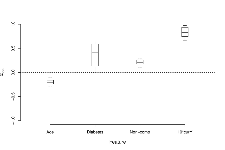
Figure 6: Posterior distribution (5th, 25th, 50th, 75th, 95th percentiles) of optimal feature weights $\mbox{\boldmath$\alpha$}_{opt}$ for the HP data analysis. The features are age (standardized), diabetes (with diabetes=1 and without diabetes=0) non-compliance ($\log(|\delta_{t-1}-A_{t-1}|+1))$, and current response ($Y_{t-1}$).

Furthermore, to explore the effects of choosing a linear function of the subject characteristics and current disease status as the risk score, we updated the policy with a quadratic term of current disease status (the most important feature) in constructing the risk score. The estimated risk score is $R_{t}=-0.38X_{3}+0.55X_{4}+0.25\log(|\delta_{t-1}-A_{t-1}|+1)+3.2Y_{t-1}+63Y_{t-1}^{2}$, with the value $-0.0101$, which is very close to the value $-0.0102$ corresponding to the optimal policy under the class of policies with only linear function of the features. Hence, we advocate using only linear features for this dataset.

8 Conclusions

Motivated to address the shortcomings of the classic 6-month recall interval in periodontal treatment allocations, we present a policy-optimized recommendation engine using BNP that exhibits superior performance, compared to alternatives. We show using simulation studies that the proposed method provides a valid posterior inference, and can reliably identify the optimal policy. Applying the method to the HP data, we find that the optimal policy recommends more frequent visits for young, unhealthy non-compliers, and that following this policy could lead to a substantial reduction in PD.

A number of computerized periodontal risk assessment tools are currently available (Page et al., 2003; Persson et al., 2003). For example, the Cigna PD self-assessment tool available at https://www.cigna.com/healthwellness/tools/periodontal-quiz-en considers subject-specific inputs through a questionnaire, and combines information from the PD fact sheet of the American Academy of Periodontology to calculate a simple ordinal risk score (low, low to moderate, moderate, or high), without any guidance towards recall intervals. There exists a number of popular chairside software in practice-based dentistry (such as Patterson’s Eaglesoft®) that record and display data. Supplementing these tools with an evidence-based recommendation system for periodontal recalls would aid practitioners.

A limitation of our analysis is that we use periodontal pocket depth (PPD) rather than the most reliable endpoint (AAP, 2005), the clinical attachment level (CAL). Site-level full mouth CAL assessment in a practice-based observational data setting like ours is time-consuming and technically demanding (Michalowicz et al., 2013). For example, in the HP dataset, CAL is computed only for the mid-buccal and mid-lingual sites, whereas, the PPD is calculated for all 6 sites on each tooth (if that tooth is present). Also, since CAL is computed from two other measures, it is more prone to error, and less reproducible than PPD (Osbom et al., 1992; Hill et al., 2006). Hence, we considered thresholded site-level PPD in addition to missing tooth to compute the proportion subject-level endpoints. The missing tooth in our analysis is assumed missing due to past incidence of PD, and the error generated from the apparent misclassification of the missingness source (such as, tooth falling out due to mechanical injury) is usually negligible while analyzing large observational databases. Should CAL and PPD measures become available for all sites (in other databases), our framework can readily incorporate this information. In addition, to reduce computational burden, our present policy only considers recall intervals of 3 and 9 months. Our method can be easily extended to more than two possible actions by adding thresholds to the risk score. Computationally, estimating an optimal threshold parameter should be similar to estimating a feature weight. Therefore, the proposed decision framework is quite general, and can be adapted to the specific needs of the practitioner.

To the best of our knowledge, this is the first study to cast the century-old debate on periodontal recall intervals into a DTR stochastic framework. Our recommendation tool is derived from a specific US midwestern population, and it’s generalizability should be tried with caution. Longitudinal PD databases from other practice-based settings (such as Kaiser Permanente®) maybe combined with the current HP database to refine findings. Furthermore, our present recall engine is geared exclusively towards PD assessment; and do not include (dental) caries risk, although evidence suggest that they may occur simultaneously (Mattila et al., 2010). These are potential directions for future work, to be pursued elsewhere.

References

- AAP (2001) AAP (2001). Glossary of Periodontal Terms. American Academy of Periodontology, Chicago, IL, 4 edition.
- AAP (2005) AAP (2005). American academy of periodontology task force report on the update to the 1999 classification of periodontal diseases and conditions. Journal of Periodontology 86, 835–838.
- Almirall et al. (2014) Almirall, D., Nahum-Shani, I., Sherwood, N. E., and Murphy, S. A. (2014). Introduction to SMART designs for the development of adaptive interventions: With application to weight loss research. Translational Behavioral Medicine 4, 260–274.
- Arjas and Saarela (2010) Arjas, E. and Saarela, O. (2010). Optimal dynamic regimes: Presenting a case for predictive inference. The International Journal of Biostatistics 6, Article 10.
- Axelsson et al. (1991) Axelsson, P., Lindhe, J., and Nyström, B. (1991). On the prevention of caries and periodontal disease. Journal of Clinical Periodontology 18, 182–189.
- CDC (2010) CDC (2010). Oral health: Preventing cavities, gum disease, tooth loss, and oral cancers at a glance 2011. CDC, Division of Oral Health, National Center for Chronic Disease Prevention and Health Promotion, Atlanta, GA .
- Chakraborty and Moodie (2013) Chakraborty, B. and Moodie, E. E. (2013). Statistical Methods for Dynamic Treatment Regimes. Springer.
- Ciarleglio et al. (2015) Ciarleglio, A., Petkova, E., Ogden, R. T., and Tarpey, T. (2015). Treatment decisions based on scalar and functional baseline covariates. Biometrics 71, 884–894.
- Cleveland and Devlin (1988) Cleveland, W. S. and Devlin, S. J. (1988). Locally weighted regression: an approach to regression analysis by local fitting. Journal of the American Statistical Association 83, 596–610.
- Davenport et al. (2003) Davenport, C., Elley, K., Fry-Smith, A., Taylor-Weetman, C., and Taylor, R. (2003). The effectiveness of routine dental checks: a systematic review of the evidence base. British Dental Journal 195, 87–98.
- Fardal et al. (2004) Fardal, Ø., Johannessen, A. C., and Linden, G. J. (2004). Tooth loss during maintenance following periodontal treatment in a periodontal practice in norway. Journal of Clinical Periodontology 31, 550–555.
- Fenol and Mathew (2010) Fenol, A. and Mathew, S. (2010). Compliance to recall visits by patients with periodontitis – Is the practitioner responsible? Journal of Indian Society of Periodontology 14, 106–108.
- Ferguson (1973) Ferguson, T. S. (1973). A Bayesian analysis of some nonparametric problems. The Annals of Statistics 1, 209–230.
- Giannobile et al. (2013) Giannobile, W. V., Braun, T. M., Caplis, A. K., Doucette-Stamm, L., Duff, G. W., and Kornman, K. S. (2013). Patient stratification for preventive care in dentistry. Journal of Dental Research 92, 694–701.
- Gramacy and Lee (2012) Gramacy, R. B. and Lee, H. K. (2012). Cases for the nugget in modeling computer experiments. Statistics and Computing 22, 713–722.
- Guan et al. (2016) Guan, Q., Laber, E. B., and Reich, B. J. (2016). Discussion of “Bayesian nonparametric estimation for dynamic treatment regimes with sequential transition times”. Journal of the American Statistical Association 111, 936–942.
- Hill et al. (2006) Hill, E. G., Slate, E. H., Wiegand, R. E., Grossi, S. G., and Salinas, C. F. (2006). Study design for calibration of clinical examiners measuring periodontal parameters. Journal of Periodontology 77, 1129–1141.
- Holtfreter et al. (2015) Holtfreter, B., Albandar, J. M., Dietrich, T., Dye, B. A., Eaton, K. A., Eke, P. I., Papapanou, P. N., and Kocher, T. (2015). Standards for reporting chronic periodontitis prevalence and severity in epidemiologic studies: Proposed standards from the joint eu/usa periodontal epidemiology working group. Journal of Clinical Periodontology 42, 407–412.
- Jones et al. (1998) Jones, D. R., Schonlau, M., and Welch, W. J. (1998). Efficient global optimization of expensive black-box functions. Journal of Global Optimization 13, 455–492.
- Kornman and Duff (2012) Kornman, K. and Duff, G. (2012). Personalized medicine will dentistry ride the wave or watch from the beach? Journal of Dental Research 91, S8–S11.
- Kosorok and Moodie (2015) Kosorok, M. R. and Moodie, E. E. (2015). Adaptive Treatment Strategies in Practice: Planning Trials and Analyzing Data for Personalized Medicine, volume 21. SIAM.
- Laber and Zhao (2015) Laber, E. and Zhao, Y. (2015). Tree-based methods for individualized treatment regimes. Biometrika 102, 501–514.
- Laber et al. (2014) Laber, E. B., Lizotte, D. J., and Ferguson, B. (2014). Set-valued dynamic treatment regimes for competing outcomes. Biometrics 70, 53–61.
- Laber et al. (2014) Laber, E. B., Lizotte, D. J., Qian, M., Pelham, W. E., and Murphy, S. A. (2014). Dynamic treatment regimes: Technical challenges and applications. Electronic Journal of Statistics 8, 1225–1272.
- Laber and Staicu (2016) Laber, E. B. and Staicu, A.-M. (2016). Functional feature construction for personalized treatment regimes. Submitted 1, 1–30.
- Laber et al. (2018) Laber, E. B., Wu, F., Munera, C., Lipkovich, I., Colucci, S., and Ripa, S. (2018). Identifying optimal dosage regimes under safety constraints: An application to long term opioid treatment of chronic pain. Statistics in Medicine 37, 1407–1418.
- Lakkaraju and Rudin (2016) Lakkaraju, H. and Rudin, C. (2016). Learning cost-effective treatment regimes using Markov decision processes. arXiv preprint arXiv:1610.06972 .
- Linn et al. (2016) Linn, K., Laber, E., and Stefanski, L. (2016). Estimation of dynamic treatment regimes for complex outcomes: Balancing benefits and risks. In Kosorok, M. R. and Moodie, E. E. M., editors, Adaptive Treatment Strategies in Practice: Planning Trials and Analyzing Data for Personalized Medicine, chapter 15, pages 249–262. ASA-SIAM, Philadelphia.
- Lizotte and Laber (2016) Lizotte, D. J. and Laber, E. B. (2016). Multi-objective Markov decision processes for data-driven decision support. Journal of Machine Learning Research 17, 1–28.
- Lövdal et al. (1961) Lövdal, A., Arno, A., Schei, O., and Werhaug, J. (1961). Combined effect of subgingival scaling and controlled oral hygiene on the incidence of gingivitis. Acta Odontologica Scandinavica 19, 537–555.
- Lu et al. (2016) Lu, X., Nahum-Shani, I., Kasari, C., Lynch, K. G., Oslin, D. W., Pelham, W. E., Fabiano, G., and Almirall, D. (2016). Comparing dynamic treatment regimes using repeated-measures outcomes: modeling considerations in SMART studies. Statistics in Medicine 35, 1595–1615.
- Luedtke and van der Laan (2016) Luedtke, A. R. and van der Laan, M. J. (2016). Optimal individualized treatments in resource-limited settings. The International Journal of Biostatistics 12, 283–303.
- Mason et al. (2003) Mason, R. L., Gunst, R. F., and Hess, J. L. (2003). Statistical Design and Analysis of Experiments: With Applications to Engineering and Science, volume 474. John Wiley & Sons, 2 edition.
- Mattila et al. (2010) Mattila, P. T., Niskanen, M. C., Vehkalahti, M. M., Nordblad, A., and Knuuttila, M. L. (2010). Prevalence and simultaneous occurrence of periodontitis and dental caries. Journal of Clinical Periodontology 37, 962–967.
- Mealey and Oates (2006) Mealey, B. L. and Oates, T. W. (2006). Diabetes mellitus and periodontal diseases. Journal of Periodontology 77, 1289–1303.
- Mettes (2005) Mettes, D. (2005). Insufficient evidence to support or refute the need for 6-monthly dental check-ups. Evidence-based Dentistry 6, 62–63.
- Michalowicz et al. (2013) Michalowicz, B. S., Hodges, J. S., and Pihlstrom, B. L. (2013). Is change in probing depth a reliable predictor of change in clinical attachment loss? The Journal of the American Dental Association 144, 171–178.
- Montgomery (2008) Montgomery, D. C. (2008). Design and Analysis of Experiments. John Wiley & Sons.
- Murphy (2003) Murphy, S. A. (2003). Optimal dynamic treatment regimes. Journal of the Royal Statistical Society: Series B (Statistical Methodology) 65, 331–355.
- Murray et al. (2017) Murray, T. A., Thall, P. F., Yuan, Y., McAvoy, S., and Gomez, D. R. (2017). Robust treatment comparison based on utilities of semi-competing risks in non-small-cell lung cancer. Journal of the American Statistical Association 112, 11–23.
- Nyman et al. (1975) Nyman, S., Rosling, B., and Lindhe, J. (1975). Effect of professional tooth cleaning on healing after periodontal surgery. Journal of Clinical Periodontology 2, 80–86.
- Orellana et al. (2010) Orellana, L., Rotnitzky, A., and Robins, J. M. (2010). Dynamic regime marginal structural mean models for estimation of optimal dynamic treatment regimes, part I: Main content. The International Journal of Biostatistics 6, Article 8.
- Osbom et al. (1992) Osbom, J. B., Stoltenberg, J. L., Huso, B. A., Aeppli, D. M., and Pihlstrom, B. L. (1992). Comparison of measurement variability in subjects with moderate periodontitis using a conventional and constant force periodontal probe. Journal of Periodontology 63, 283–289.
- Page et al. (2003) Page, R. C., Martin, J., Krall, E. A., Mancl, L., and Garcia, R. (2003). Longitudinal validation of a risk calculator for periodontal disease. Journal of Clinical Periodontology 30, 819–827.
- Persson et al. (2003) Persson, G. R., Mancl, L. A., Martin, J., and Page, R. C. (2003). Assessing periodontal disease risk: a comparison of clinicians’ assessment versus a computerized tool. The Journal of the American Dental Association 134, 575–582.
- Riley et al. (2013) Riley, P., Worthington, H. V., Clarkson, J. E., and Beirne, P. V. (2013). Recall intervals for oral health in primary care patients (Review). The Cochrane Library: Cochrane Database of Systematic Reviews 12, 1–31.
- Robins (1986) Robins, J. (1986). A new approach to causal inference in mortality studies with a sustained exposure period application to control of the healthy worker survivor effect. Mathematical Modelling 7, 1393–1512.
- Robins et al. (2008) Robins, J., Orellana, L., and Rotnitzky, A. (2008). Estimation and extrapolation of optimal treatment and testing strategies. Statistics in Medicine 27, 4678–4721.
- Robins (2004) Robins, J. M. (2004). Optimal structural nested models for optimal sequential decisions. In Proceedings of the second Seattle Symposium in Biostatistics, pages 189–326. Springer.
- Rosén et al. (1999) Rosén, B., Olavi, G., Badersten, A., Rönström, A., Söderholm, G., and Egelberg, J. (1999). Effect of different frequencies of preventive maintenance treatment on periodontal conditions. 5-year observations in general dentistry patients. Journal of Clinical Periodontology 26, 225–233.
- Roustant et al. (2012) Roustant, O., Ginsbourger, D., and Deville, Y. (2012). Dicekriging, diceoptim: Two r packages for the analysis of computer experiments by kriging-based metamodelling and optimization. Journal of Statistical Software 51, 54p.
- Ryu et al. (2007) Ryu, D., Sinha, D., Mallick, B., Lipsitz, S. R., and Lipshultz, S. E. (2007). Longitudinal studies with outcome-dependent follow-up: Models and Bayesian regression. Journal of the American Statistical Association 102, 952–961.
- Schulte et al. (2014) Schulte, P. J., Tsiatis, A. A., Laber, E. B., and Davidian, M. (2014). Q-and A-learning methods for estimating optimal dynamic treatment regimes. Statistical Science 29, 640–661.
- Sethuraman (1994) Sethuraman, J. (1994). A constructive definition of Dirichlet priors. Statistica Sinica 4, 639–650.
- Shortreed and Moodie (2012) Shortreed, S. M. and Moodie, E. E. (2012). Estimating the optimal dynamic antipsychotic treatment regime: evidence from the sequential multiple-assignment randomized Clinical Antipsychotic Trials of Intervention and Effectiveness schizophrenia study. Journal of the Royal Statistical Society: Series C (Applied Statistics) 61, 577–599.
- Teich (2013) Teich, S. T. (2013). Risk assessment-based individualized treatment (RABIT): a comprehensive approach to dental patient recall. Journal of Dental Education 77, 448–457.
- Tobin (1958) Tobin, J. (1958). Estimation of relationships for limited dependent variables. Econometrica: Journal of the Econometric Society 26, 24–36.
- van der Laan and Petersen (2007) van der Laan, M. J. and Petersen, M. L. (2007). Causal effect models for realistic individualized treatment and intention to treat rules. The International Journal of Biostatistics 3, Article 3.
- Wall, Thomas and Guay, Albert (2016) Wall, Thomas and Guay, Albert (2016). The Per-Patient Cost of Dental Care, 2013: A Look Under the Hood. available at: http://www.ada.org/~/media/ADA/Science%20and%20Research/HPI/Files/HPIBrief_0316_4.pdf (Health Policy Institute Research Brief, American Dental Association, March 2016).
- Wang et al. (2018) Wang, Y., Fu, H., and Zeng, D. (2018). Learning optimal personalized treatment rules in consideration of benefit and risk: with an application to treating type 2 diabetes patients with insulin therapies. Journal of the American Statistical Association 113, 1–13.
- Wu et al. (2015) Wu, F., Laber, E. B., Lipkovich, I. A., and Severus, E. (2015). Who will benefit from antidepressants in the acute treatment of bipolar depression? A reanalysis of the STEP-BD study by Sachs et al. 2007, using Q-learning. International Journal of Bipolar Disorders 3, 1–11.
- Xu et al. (2016) Xu, Y., Müller, P., Wahed, A. S., and Thall, P. F. (2016). Bayesian nonparametric estimation for dynamic treatment regimes with sequential transition times. Journal of the American Statistical Association 111, 921–950.
- Zanardi et al. (2012) Zanardi, G., Proffit, W. R., and Frazier-Bowers, S. A. (2012). The future of dentistry: how will personalized medicine affect orthodontic treatment? Dental Press Journal of Orthodontics 17, 3–6.
- Zhang et al. (012b) Zhang, B., Tsiatis, A. A., Davidian, M., Zhang, M., and Laber, E. (2012b). Estimating optimal treatment regimes from a classification perspective. Stat 1, 103–114.
- Zhang et al. (012a) Zhang, B., Tsiatis, A. A., Laber, E. B., and Davidian, M. (2012a). A robust method for estimating optimal treatment regimes. Biometrics 68, 1010–1018.
- Zhang et al. (2013) Zhang, B., Tsiatis, A. A., Laber, E. B., and Davidian, M. (2013). Robust estimation of optimal dynamic treatment regimes for sequential treatment decisions. Biometrika 100, 681–694.
- Zhang et al. (2015) Zhang, Y., Laber, E. B., Tsiatis, A., and Davidian, M. (2015). Using decision lists to construct interpretable and parsimonious treatment regimes. Biometrics 71, 895–904.
- Zhao et al. (2012) Zhao, Y., Zeng, D., Rush, A. J., and Kosorok, M. R. (2012). Estimating individualized treatment rules using outcome weighted learning. Journal of the American Statistical Association 107, 1106–1118.
- Zhao et al. (2015) Zhao, Y.-Q., Zeng, D., Laber, E. B., and Kosorok, M. R. (2015). New statistical learning methods for estimating optimal dynamic treatment regimes. Journal of the American Statistical Association 110, 583–598.
- Zhou and Kosorok (2017) Zhou, X. and Kosorok, M. R. (2017). Augmented outcome-weighted learning for optimal treatment regimes. arXiv preprint arXiv:1711.10654 .