The Fundamental Theorem of Algebra in ACL2

Abstract

We report on a verification of the Fundamental Theorem of Algebra in ACL2(r). The proof consists of four parts. First, continuity for both complex-valued and real-valued functions of complex numbers is defined, and it is shown that continuous functions from the complex to the real numbers achieve a minimum value over a closed square region. An important case of continuous real-valued, complex functions results from taking the traditional complex norm of a continuous complex function. We think of these continuous functions as having only one (complex) argument, but in ACL2(r) they appear as functions of two arguments. The extra argument is a “context”, which is uninterpreted. For example, it could be other arguments that are held fixed, as in an exponential function which has a base and an exponent, either of which could be held fixed. Second, it is shown that complex polynomials are continuous, so the norm of a complex polynomial is a continuous real-valued function and it achieves its minimum over an arbitrary square region centered at the origin. This part of the proof benefits from the introduction of the “context” argument, and it illustrates an innovation that simplifies the proofs of classical properties with unbound parameters. Third, we derive lower and upper bounds on the norm of non-constant polynomials for inputs that are sufficiently far away from the origin. This means that a sufficiently large square can be found to guarantee that it contains the global minimum of the norm of the polynomial. Fourth, it is shown that if a given number is not a root of a non-constant polynomial, then it cannot be the global minimum. Finally, these results are combined to show that the global minimum must be a root of the polynomial. This result is part of a larger effort in the formalization of complex polynomials in ACL2(r).

1 Introduction

In this paper, we describe a verification of the Fundamental Theorem of Algebra (FTA) in ACL2(r). That is, we prove that if $p$ is a non-constant, complex polynomial with complex coefficients, then there is some complex number $z$ such that $p(z)=0$. The proof follows the outline of the first proof in [4], and it is a formal version of d’Alembert’s proof of 1746 [2], which is illustrated (literally) in [12].

Figure 1 provides an outline of the proof, which comprises three main strands. First (step 1 in Figure 1), we show that continuous functions from the complex plane to the reals always achieve a minimum value in a closed, bounded, rectangular region. The consequence to the FTA is that if $p$ is a complex polynomial, then the function mapping $z\in\mathbb{C}$ to $||p(z)||$, where $||\cdot||$ denotes the traditional complex norm, achieves a minimum value in a square region centered at the origin (steps 2, 3, and 5). Second (step 4), we show that the norm of polynomials is dominated by the term of highest power. In particular, if $p(z)=a_{\_}nz^{n}+a_{\_}{n-1}z^{n-1}+\cdots+a_{\_}0$, then $\frac{1}{2}||a_{\_}n||\,||z||^{n}<||p(z)||<\frac{3}{2}||a_{\_}n||\,||z||^{n}$ for sufficiently large $z$. These two facts can be combined to show that the global minimum of a polynomial (norm) must be enclosed in a possibly large region around the origin, so the polynomial must achieve this global minimum. The third strand (step 6), known as d’Alembert’s Lemma, states that if $p$ is a complex polynomial and $z$ is such that $p(z)\neq 0$, then there is some $z_{\_}0$ such that $||p(z_{\_}0)||<||p(z)||$. This implies that the global minimum guaranteed by the previous lemmas must be a root of the polynomial (step 7).

To our knowledge, this is the first proof of the Fundamental Theorem of Algebra in the Boyer–Moore family of theorem provers, but it has been proved earlier in other theorem provers, e.g., Mizar [10], HOL [9], and Coq [8].

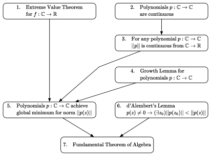
Figure 1: Proof Outline

2 Continuity and the Extreme Value Theorem

2.1 Continuous Functions

We begin the proof of the FTA with a proof of the Extreme Value Theorem for complex functions. The first step is to define the notion of continuity for complex functions, and this follows the pattern used before for real functions [7]. In particular, we say that $f$ is continuous if for any standard number $z$, $f(z)$ is close to $f(z_{\_}*)$ for any $z_{\_}*$ that is close to $z$. To be precise, two complex numbers are “close” if both the real and imaginary parts of their difference are infinitesimal. This also implies that the distance between the two points is infinitesimal.

We also introduced in ACL2(r) the notion of a continuous function from the complex to the real numbers, and we proved that if both $f:\mathbb{C}\rightarrow\mathbb{C}$ and $g:\mathbb{C}\rightarrow\mathbb{R}$ are continuous, then so is $g\circ f:\mathbb{C}\rightarrow\mathbb{R}$. Moreover, we proved that the function given by the traditional complex norm, $||a+bi||=\sqrt{a^{2}+b^{2}}$, is continuous. So for any continuous function $f:\mathbb{C}\rightarrow\mathbb{C}$, the function from $\mathbb{C}$ to $\mathbb{R}$ given by $h(z)=||f(z)||$ is continuous.

An important difference from the development in [7] is that continuous functions in this paper have two arguments in ACL2, even though we think of them as functions of only one variable. This is similar to the way the function $x^{n}$ and $a^{x}$ are introduced in elementary calculus. Those functions are thought of as functions of the single variable $x$, and the derivatives are given as $nx^{n-1}$ and $a^{x}\ln{a}$, even though both functions are simply slices of the bivariate function $x^{y}$.

In ACL2(r), we introduce the continuous function ccfn using encapsulate as (ccfn context z), where the argument z is the one that is allowed to vary, whereas context is the argument that is held fixed. The non-standard definition of continuity that we use here requires that close points be mapped to close values, but only for standard z. Similarly, we require that close points are mapped to close values only when both z and context are standard.

The context argument plays an important role, which can be illustrated by the continuity of polynomials. Consider, for example, a proof that the function $x^{n}$ is continuous. This would appear to be easy to prove by induction as follows:

1. $x^{0}$ is a constant function, so it is definitely continuous.

2. $x^{n}=x^{n-1}\cdot x$, and $x^{n-1}$ is continuous from the induction hypothesis, and so is the product of continuous functions.

However, this does not work. The formal definition of continuity uses the non-classical notions of $close$: $standard(x)\wedge close(x,x_{\_}0)\rightarrow close(x^{n},x_{\_}0^{n})$. But ACL2(r) restricts induction on non-classical functions to standard values of the arguments. In this particular case, we could prove that $x^{n}$ is continuous, but only for standard values of $n$, as was done in [11].

Setting that aside for now, we can imagine what would happen if we could establish (somehow) that complex polynomials are continuous. The next step in the proof would be to show that since $p(z)$ is continuous in the complex plane, then $||p(z)||$ is continuous from $\mathbb{C}$ to $\mathbb{R}$, and this could be done by functionally instantiating the previous result about norms of continuous functions. Once more, however, we run into a major complication. The problem is that we want to say this about all polynomials, not just about a specific polynomial $p$. For example, we could use this approach to show that the norm of the following polynomial is continuous:

⬇

(defun p(z)

(+ 1 (* #c(0 1) z) (* 3 z z)))

But that would lead to a proof that the polynomial $p$ has a root, not that all polynomials have roots. To reason about all polynomials, we use a data structure that can represent any polynomial and an evaluator function that can compute the value of a given polynomial at a given point. For example, the polynomial above is represented with the list (1 #c(0 1) 3), and the function eval-polynomial is defined so that (eval-polynomial ’(1 #c(0 1) 3) z) = (p z). But we cannot use functional instantiation to show that the norm of eval-polynomial is continuous, because the formal statement of continuity uses the non-classical notion of $close$. ACL2(r) restricts functional instantiation so that pseudo-lambda expressions cannot be used in place of functions when the theorem to be proved uses non-classical functions.

It should be noted that both of these restrictions are necessary! For example, $x^{n}$ is “obviously” continuous, but what happens when $n$ is large? Suppose that $x=1+\epsilon$, where $\epsilon$ is small, so that $1$ and $1+\epsilon$ are close. From the binomial theorem, $(1+\epsilon)^{n}=1+n\epsilon+\cdots$. The thing is that if $n$ is large, $n\epsilon$ is not necessarily small. For instance, if $n=1/\epsilon$, then $n\epsilon=1$, and $(1+\epsilon)^{n}>2$, so it is not close to $1^{n}=1$. Yes, $x^{n}$ is continuous, but the non-standard definition of continuity only applies when $x$ and $n$ are standard.

Similarly, the restriction for pseudo-lambda expressions is crucial. Consider, for example, the theorem that $f(x)$ is standard when $x$ is standard. This is true, but we could not use it to show that $x+y$ is standard when $x$ is standard by functionally instantiating $\lambda x.x+y$ for $f$. The proposed theorem is just not true when, for example, $x=0$ and $y=\epsilon$.

So these restrictions are important for soundness, and we have to find a way to live with them. In both cases, the key to doing so is the context argument. Consider eval-polynomial, which has two arguments: the polynomial poly and the point z. Here, poly plays the role of context. Notice how poly is “held fixed” when we say that a polynomial is continuous over the complex numbers. Because the context argument is used to refer to an arbitrary polynomial, there is no need to use a pseudo-lambda expression to introduce poly, so we can instantiate the theorem that $||eval\text{-}polynomial(poly,z)||$ is continuous from $\mathbb{C}$ to $\mathbb{R}$ without running afoul of the restriction on free variables in functional instantiation of non-classical formulas.

That leaves the continuity of polynomial functions to deal with. Here we want to show that when $z$ is standard and close to $z_{\_}0$, $eval\text{-}polynomial(poly,z)$ is also close to $eval\text{-}polynomial(poly,z_{\_}0)$. Again, the context argument plays a major role, because the proof obligation of the encapsulate is actually weaker. It says that $eval\text{-}polynomial(poly,z)$ must be close to $eval\text{-}polynomial(poly,z_{\_}0)$ only when both $poly$ and $z$ are standard—and in that case we can use induction to prove the result. But notice that $poly$ is a list, so it is standard when it consists of standard elements and has standard length, which is not the case for all polynomials. As was the case before, this is the best we could expect. Consider, for instance, the polynomial $p(z)=Nz$ where $N$ is a large constant. Then $p(0)=0$ but $p(\epsilon)=N\epsilon$ is not necessarily close to $0$.

But what about the Fundamental Theorem of Algebra? Does this mean that we can only prove this theorem for standard arguments? Thankfully, that is not the case. We can proceed with the proof of the Fundamental Theorem of Algebra for all polynomials because of the principle of transfer. This works because the statement of the Fundamental Theorem of Algebra is classical: if $p$ is a non-constant, complex polynomial with complex coefficients, then there is some complex number $z$ such that $p(z)=0$. Notice that statement does not mention concepts like $standard$, $close$, or $small$. So if it holds for all standard polynomials $poly$, it also holds for all polynomials, even the non-standard ones. The same holds for other classical properties, such as the Extreme Value Theorem.

We believe that this approach is significantly cleaner than what we have done before. For example, in [11] we used something similar to the context argument, but the extra arguments were numbers. This means we were reasoning about functions of, say, 10 variables while holding 9 fixed, and if another fixed parameter was needed, we would have to redefine the constrained continuous function. In contrast, the context parameter is only required to be standard, not necessarily a number. So we could use it, for example, to hold a list of 9 fixed dimensions in one setting, and 10 fixed dimensions in another one. The constrained function does not need to change to accommodate the extra dimension, and nor do any of the generic theorems that were previously proved, e.g., the Extreme Value Theorem. As long as all the other dimensions are fixed, they can be added to the context.

A more traditional way of dealing with this problem is to realize that continuity itself is a classical notion, so we can use a classical constrained function to introduce the notion in ACL2(r). This is what we did in [3] where we explored equivalent definitions of continuity and showed how versions of theorems like the Intermediate Value Theorem could be proved for the classical and non-classical definitions of continuity. But we also think that the approach used here works better, because there is no need to have both classical and non-classical versions of all the theorems. Rather, the necessary theorems can be proved using the non-classical definitions, which are simpler to use in a theorem prover known for rewriting and induction, and then instantiating these (classical) theorems when needed. That is exactly what we do here, where we prove the Extreme Value Theorem using the intuitive notions of $close$, and then instantiate this theorem for all polynomials using the fixed context parameter—without having to establish that polynomials satisfy the $\epsilon$–$\delta$ definition of continuity.

2.2 Proof of the Extreme Value Theorem

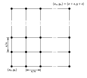
Figure 2: Proof of Extreme Value Theorem

We now turn attention to the proof of the Extreme Value Theorem for continuous functions from the complex to the real numbers. The proof is similar in principle to the analogous theorem for real functions, although it is more complicated since the relevant region is a square instead of an interval. In both proofs, we use a constrained function to stand for all possible continuous functions. In the earlier proof, we used rcfn to stand for a real continuous function. We also use the name ccfn to stand for an arbitrary complex continuous function. In this section, we will be using crvcfn which is a constrained complex, real-valued, continuous function.

Figure 2 shows the basic idea of the proof. The square of size $s\times s$ is subdivided into regions and the value of the function is found at the points in an $(n+1)\times(n+1)$ grid. Using recursion, it is straightforward to find the point on the grid where the function $f$ has a minimal value, say $z_{\_}m=(x_{\_}i,y_{\_}j)$.

At this point, we can assume that $(x_{\_}0,y_{\_}0)$ and $s$ are both standard, so the square defined by the points $(x_{\_}0,y_{\_}0)$ and $(x_{\_}n,y_{\_}n)$ is also standard. This means that if $z$ is inside the square, so is the standard part of $z$. In particular, the standard part of any of the points in the grid must be inside the square region. And from this point on, we can also assume that $n$ is a large number, so that adjacent points on the grid are a distance at most $\sqrt{2}\,s/n$ apart, hence close to each other.

Since all the grid points are inside a standard square, they must be limited. This justifies using the non-standard definitional principle defun-std to define the minimum as the standard part of $z_{\_}m$, written as ${}^{*}z_{\_}m$ or $standardpart(z_{\_}m)$. The non-standard definitional principle assures us that the minimum is precisely ${}^{*}z_{\_}m$, but only when $x_{\_}0$, $y_{\_}0$, and $s$ are standard.

Now, consider any standard point $z$ that lies inside the square region. It must be inside one of the grid cells, and since adjacent grid points are close to each other, $z$ must also be close to the grid points in the enclosing cell, and since it is standard it must be the standard part of those grid points—points that are close to each other have the same standard part. So suppose that $z$ is close to $(x_{\_}k,y_{\_}l)$—as just observed, it must be close to some point on the grid. There are two cases to consider. If this point happens to be equal to $z_{\_}m=(x_{\_}i,y_{\_}j)$, the minimum point on the grid, then as just observed, it must be the case that its standard part ${}^{*}z_{\_}m$, must be equal to $z$. So it follows trivially that $f({}^{*}z_{\_}m)\leq f(z)$. Conversely, if $(x_{\_}k,y_{\_}l)\neq(x_{\_}i,y_{\_}j)=z_{\_}m$, then it must be the case that $f(z_{\_}m)=f(x_{\_}i,y_{\_}j)\leq f(x_{\_}k,y_{\_}l)$, because $z_{\_}m$ was chosen as the minimum point on the grid. Taking standard parts of both sides shows that ${}^{*}f(z_{\_}m)={}^{*}f(x_{\_}i,y_{\_}j)\leq{}^{*}f(x_{\_}k,y_{\_}l)$. It is only necessary to prove that ${}^{*}f(z_{\_}0)=f({}^{*}z_{\_}0)$ for all $z_{\_}0$, and again we have established that $f({}^{*}z_{\_}m)\leq f(z)$. So in either case, $f({}^{*}z_{\_}m)$ is at most the value of $f(z)$ for any standard $z$ in the square. Using the transfer principle with defthm-std, we generalized this statement to prove that ${}^{*}z_{\_}m$ is the minimum value over all points in the square region from $(x_{\_}0,y_{\_}0)$ to $(x_{\_}0+s,y_{\_}0+s)$, for all values of $x_{\_}0$, $y_{\_}0$, and $s$, not just the standard ones.

Although this proof is carried out for arbitrary continuous functions, the intent is to use functional instantiation to show that some specific function achieves its minimum. Thus, it is very helpful to use quantifiers to state the Extreme Value Theorem, so that a future use via functional instantiation does not need to recreate the functions used to search the grid, for example. The following definition captures what it means for the point zmin to be the minimum point inside the square or side length s with lower-left corner at z0:

⬇

(defun-sk is-minimum-point-in-region (context zmin z0 s)

(forall (z)

(implies (and (acl2-numberp z)

(acl2-numberp z0)

(realp s)

(< 0 s)

(inside-region-p

z

(cons (interval (realpart z0)

(+ s (realpart z0)))

(interval (imagpart z0)

(+ s (imagpart z0))))))

(<= (crvcfn context zmin) (crvcfn context z)))))

The Extreme Value Theorem, then, simply adds that there is some value of zmin that makes this true. The existence is captured with the following definition:

⬇

(defun-sk achieves-minimum-point-in-region (context z0 s)

(exists (zmin)

(implies (and (acl2-numberp z0)

(realp s)

(< 0 s))

(and (inside-region-p

zmin

(cons (interval (realpart z0)

(+ s (realpart z0)))

(interval (imagpart z0)

(+ s (imagpart z0)))))

(is-minimum-point-in-region context

zmin z0 s)))))

Using this definition, the Extreme Value Theorem can be stated simply as follows:

⬇

(defthm minimum-point-in-region-theorem-sk

(implies (and (acl2-numberp z0)

(realp s)

(< 0 s)

(inside-region-p z0 (crvcfn-domain))

(inside-region-p (+ z0 (complex s s)) (crvcfn-domain)))

(achieves-minimum-point-in-region context z0 s))

:hints ...)

It is then a simple matter to functionally instantiate this theorem for any polynomial.

3 Growth Lemma for Polynomials

In the previous section, we proved the Extreme Value Theorem for continuous functions from $\mathbb{C}$ to $\mathbb{R}$. In this section, we turn our attention to the values $||p(z)||$ for polynomials $p$, and we are primarily interested in $||p(z)||$ when $z$ is sufficiently far from the origin.

Let $p(z)$ be given by $p(z)=a_{\_}0+a_{\_}1z+a_{\_}2z^{2}+\cdots+a_{\_}nz^{n}$, where $a_{\_}n\neq 0$. It follows that

$$||p(z)||=||a_{\_}0+a_{\_}1z+a_{\_}2z^{2}+\cdots+a_{\_}nz^{n}||.$$

Using induction and the triangle inequality for $||\cdot||$, we proved that

$$||p(z)||\leq||a_{\_}0||+||a_{\_}1z||+||a_{\_}2z^{2}||+\cdots+||a_{\_}nz^{n}||.$$

The norm $||\cdot||$ behaves nicely with products. In particular, we proved that $||xy||=||x||\,||y||$, so

$$||p(z)||\leq||a_{\_}0||+||a_{\_}1||\,||z||+||a_{\_}2||\,||z^{2}||+\cdots+||a_{\_}n||\,||z^{n}||.$$

Letting $A=\max||a_{\_}i||$, it is easy to prove that

$$||p(z)||\leq A\left(||z^{0}||+||z^{1}||+||z^{2}||+\cdots+||z^{n}||\right).$$

We are only interested in the value of $||p(z)||$ when $z$ is sufficiently large, so we can limit the discussion to those values of $z$ with $||z||\geq 1$. A simple induction shows that for those $z$, $||z||\leq||z^{n}||$, so

$$||p(z)||\leq A\left(||z^{n}||+||z^{n}||+||z^{n}||+\cdots+||z^{n}||\right)=A(n+1)||z^{n}||.$$

Another simple induction shows that $||z^{n}||=||z||^{n}$, so we have that

$$||p(z)||\leq A(n+1)||z||^{n}.$$

Now, suppose that $\frac{A(n+1)}{K}\leq||z||$ for an arbitrary, real number $K$—clearly, for any fixed $K$, we can always find a $z$ large enough to make this true, since $A$ and $n$ are always fixed. Then $A(n+1)\leq K||z||$, and we have

$$||p(z)||\leq A(n+1)||z||^{n}\leq K||z||^{n+1}.$$

The last result holds for all polynomials $p$. Now we use that result to get both lower and upper bounds for any polynomial $q$. In particular, let $q(z)=a_{\_}0+a_{\_}1z+a_{\_}2z^{2}+\cdots+a_{\_}nz^{n}$. Then $q$ can be written as $q(z)=(a_{\_}0+a_{\_}1z+a_{\_}2z^{2}+\cdots+a_{\_}{n-1}z^{n-1})+a_{\_}nz^{n}.$ Applying the previous result to the polynomial in parentheses, we have that

$$q(z)\leq K||z||^{n}+||a_{\_}n||\,||z||^{n},$$

for any $K$ and $z$ such that $An\leq K||z||$. Choosing $K=||a_{\_}n||/2$, we have that

$$q(z)\leq K||z||^{n}+||a_{\_}n||\,||z||^{n}=\frac{||a_{\_}n||}{2}||z||^{n}+||a_{\_}n||\,||z||^{n}=\frac{3}{2}||a_{\_}n||\,||z||^{n}.$$

That provides a nice upper bound for $||q(z)||$. In ACL2, this can be shown as follows.

⬇

(defthm upper-bound-for-norm-poly

(implies (and (polynomial-p poly)

(< 1 (len poly))

(not (equal (leading-coeff poly) 0))

(acl2-numberp z)

(<= 1 (norm2 z))

(<= (/ (* 2

(max-norm2-coeffs (all-but-last poly))

(1- (len poly)))

(norm2 (leading-coeff poly)))

(norm2 z)))

(<= (norm2 (eval-polynomial poly z))

(* 3/2

(norm2 (leading-coeff poly))

(expt (norm2 z) (1- (len poly))))))

:hints ...)

We can find a lower bound on $||q(z)||$ by observing that

$$q(z)=a_{\_}nz^{n}-(-a_{\_}0-a_{\_}1z-a_{\_}2z^{2}+\cdots-a_{\_}{n-1}z^{n-1}),$$

and using the variant of the triangle inequality $||a-b||\geq||a|-||b||$, we have that

$$||q(z)||\geq||a_{\_}nz^{n}||-||-a_{\_}0-a_{\_}1z-a_{\_}2z^{2}+\cdots-a_{\_}{n-1}z^{n-1}||.$$

Further, since multiplying a value by $-1$ does not change its norm, we can write this as

$$||q(z)||\geq||a_{\_}nz^{n}||-||a_{\_}0+a_{\_}1z+a_{\_}2z^{2}+\cdots+a_{\_}{n-1}z^{n-1}||.$$

As we saw previously, $||a_{\_}0+a_{\_}1z+a_{\_}2z^{2}+\cdots+a_{\_}{n-1}z^{n-1}||\leq\frac{||a_{\_}n||}{2}||z||^{n}$, so

$$||q(z)||\geq||a_{\_}nz^{n}||-||a_{\_}0+a_{\_}1z+a_{\_}2z^{2}+\cdots+a_{\_}{n-1}z^{n-1}||\geq||a_{\_}nz^{n}||-\frac{||a_{\_}n||}{2}||z||^{n}=\frac{1}{2}||a_{\_}n||\,||z||^{n}.$$

This can be shown in ACL2 as follows:

⬇

(defthm lower-bound-for-norm-poly

(implies (and (polynomial-p poly)

(< 1 (len poly))

(not (equal (leading-coeff poly) 0))

(acl2-numberp z)

(<= 1 (norm2 z))

(<= (/ (* 2

(max-norm2-coeffs (all-but-last poly))

(1- (len poly)))

(norm2 (leading-coeff poly)))

(norm2 z)))

(<= (* 1/2

(norm2 (leading-coeff poly))

(expt (norm2 z) (1- (len poly))))

(norm2 (eval-polynomial poly z))))

:hints ...)

Combining the previous two results, we have shown that

$$\frac{1}{2}||a_{\_}n||\,||z||^{n}\leq||q(z)||\leq\frac{3}{2}||a_{\_}n||\,||z||^{n},$$

for values of $z$ with sufficiently large $||z||$.

Since the results hold for all $z$ with sufficiently large $||z||$, we can restrict ourselves to $z$ such that $||z||\geq 2\frac{||a_{\_}0||}{||a_{\_}n||}$. In this case, we have that

$$q(z)\geq\frac{1}{2}||a_{\_}n||\,||z||^{n}\geq\frac{1}{2}||a_{\_}n||\,||z||\geq\frac{1}{2}||a_{\_}n||\left(2\frac{||a_{\_}0||}{||a_{\_}n||}\right)=||a_{\_}0||.$$

But observe that $q(0)=a_{\_}0$, so $||q(z)||\geq||q(0)||$.

The situation is summarized in Figure 3. All points in the gray area—that is, outside of the circle—are large enough that $||q(z)||\geq||a_{\_}0||=||q(0)||$. On the other hand, the minimum point $z_{\_}m$ guaranteed by the Extreme Value Theorem lies inside the square, and since it is the minimum point inside the square, it holds that $||q(z_{\_}m)||\leq||q(0)||=||a_{\_}0||$. Combining these two statements, we have that $||q(z_{\_}m)||\leq||q(z)||$ for all $z$ whether they are inside or outside of the circle. In other words, $z_{\_}m$ is not just a minimum inside the square region. It is a global minimum for $q$.

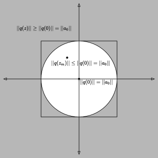
Figure 3: Local Minimum Is a Global Minimum

4 d’Alembert’s Lemma

We now prove d’Alembert’s Lemma, which states that for a non-constant polynomial $p$, if $z$ is such that $p(z)\neq 0$, then there is some $z_{\_}0$ such that $||p(z_{\_}0)||<||p(z)||$. In particular, if $p(z)\neq 0$ then $z$ cannot be a global minimum of $||p(\cdot)||$.

We prove this lemma by proceeding in a series of special cases. First, let’s assume that $a_{\_}0=1$ so that

$$p(z)=1+a_{\_}1z+a_{\_}2z^{2}+\cdots+a_{\_}nz^{n}.$$

Let $k$ be the largest index such that $a_{\_}1=a_{\_}2=\cdots=a_{\_}{k-1}=0$. We note that $k\leq n$, since we assume throughout this paper that $a_{\_}n\neq 0$. Then,

$$p(z) =1+a_{\_}kz^{k}+a_{\_}{k+1}z^{k+1}+\cdots+a_{\_}nz^{n}$$

$$=1+a_{\_}kz^{k}+z^{k+1}q(z)$$

where $q$ is a particular polynomial. Of course, this means that

$$||p(z)|| =||1+a_{\_}kz^{k}+z^{k+1}q(z)||$$

$$\leq||1+a_{\_}kz^{k}||+||z^{k+1}q(z)||$$

Suppose that $s$ is real number such that $0<s<1$, and let $z_{\_}s=\sqrt[k]{-\frac{s}{a_{\_}k}}$. We note in passing that the existence of such a $z_{\_}s$ is guaranteed by de Moivre’s lemma, which we proved as part of this effort, using the principal logarithmic function defined in [6].

⬇

(defthm de-moivre-1

(implies (and (acl2-numberp z)

(natp n))

(equal (expt z n)

(* (expt (radiuspart z) n)

(acl2-exp (* #c(0 1) n (anglepart z))))))

:hints ...)

(defthm de-moivre-2

(implies (and (acl2-numberp z)

(posp n))

(equal (expt (nth-root z n) n) z))

:hints ...)

Since $z_{\_}s=\sqrt[k]{-\frac{s}{a_{\_}k}}$, we have that

$$a_{\_}kz_{\_}s^{k}=a_{\_}k\left(\sqrt[k]{-\frac{s}{a_{\_}k}}\right)^{k}=-s.$$

So $||1+a_{\_}kz_{\_}s^{k}||=||1-s||=|1-s|=1-s$, since $s$ is real and $0<s<1$. This means that

$$||p(z_{\_}s)|| \leq||1+a_{\_}kz_{\_}s^{k}||+||z_{\_}s^{k+1}q(z_{\_}s)||$$

$$=1-s+||z_{\_}s^{k+1}q(z_{\_}s)||$$

$$=1-s+||z_{\_}s||^{k}\,||z_{\_}s||\,||q(z_{\_}s)||$$

$$=1-s+\frac{s}{||a_{\_}k||}\,||z_{\_}s||\,||q(z_{\_}s)||$$

$$=1-s\left(1-\frac{||z_{\_}s||}{||a_{\_}k||}||q(z_{\_}s)||\right)$$

It’s obvious that the term in parentheses is real and at most 1. What we want to show now is that it is actually positive and at most 1 for at least one choice of $s$, and hence $z_{\_}s$. That is, we will show that there is an $s$ such that $\frac{||z_{\_}s||}{||a_{\_}k||}||q(z_{\_}s)||<1$.

We find this $s$ by observing that whenever $z$ is such that $0<||z||<1$, then $||q(z)||\leq M(n+1)$, where $M$ is the maximum norm of the coefficients, i.e., $M=\max||a_{\_}i||$. Let $r=\frac{||z||}{||a_{\_}k||}||q(z)||$. If $q(z)=0$, then $r=0<1$. Otherwise, as long as $0<||z||<1$ and $0<||z||<\frac{||a_{\_}k||}{M(n+1)}$, we have that $r=\frac{||z||}{||a_{\_}k||}||q(z)||<\frac{||a_{\_}k||}{||a_{\_}k||M(n+1)}||q(z)||\leq\frac{1}{M(n+1)}M(n+1)=1$. So as long as $0<||z||<1$ and $0<||z||<\frac{||a_{\_}k||}{M(n+1)}$, $0\leq r<1$ (regardless of the value of $q(z)$.) Therefore,

$$||p(z)|| \leq 1-s\left(1-\frac{||z||}{||a_{\_}k||}||q(z)||\right)$$

$$\leq 1-s\left(1-r\right)$$

$$<1.$$

The last inequality follows since $0\leq r<1$, so $1-r>0$ and $s>0$. So it remains only to choose an $s$ such that $0<||z_{\_}s||<\frac{||a_{\_}k||}{M(n+1)}$. Since $z_{\_}s=\sqrt[k]{-\frac{s}{a_{\_}k}}$ this is equivalent to finding a positive number $s$ small enough such that $s<\frac{||a_{\_}k||^{k+1}}{M^{k}(n+1)^{k}}$, which is obviously possible since the right-hand side is positive. This is summarized in the ACL2 theorem below:

⬇

(defthm lowest-exponent-split-10

(implies (and (polynomial-p poly)

(equal (car poly) 1)

(< 1 (len poly))

(not (equal (leading-coeff poly) 0))

(equal (car poly) 1)

)

(< (norm2 (eval-polynomial

poly

(fta-bound-1 poly

(input-with-smaller-value

poly))))

1))

:hints ...)

The function fta-bound-1 corresponds to the choice of $x_{\_}s$, and input-with-smaller-value finds a suitable value of $s$.

To complete the proof, observe that since $||p(z_{\_}s)||<1=p(0)$, we have that 0 cannot be the global minimum. It is worth remembering that the only thing we assumed about this polynomial is that $a_{\_}0=p(0)=1$. We generalize this proof by removing this assumption and letting $a_{\_}0\neq 1$. If it happens that $a_{\_}0=0$, then $p(0)=a_{\_}0=0$ and the polynomial has a root. Otherwise, $a_{\_}0\neq 0$ and we can define the new polynomial

$$p_{\_}1(z)=1+\frac{a_{\_}1}{a_{\_}0}z+\frac{a_{\_}2}{a_{\_}0}z^{2}+\cdots+\frac{a_{\_}n}{a_{\_}0}z^{n}.$$

Notice that $p_{\_}1(z)=p(z)/a_{\_}0$, so $||p_{\_}1(z)||=||p(z)||/||a_{\_}0||$. This means that if $0$ is not a global minimum of $||p||$, it cannot be a global minimum of $||p_{\_}1||$, either.

Finally, we remove the assumption that it is at the point $z=0$ that $p(z)\neq 0$. Suppose, in fact, that $p(z_{\_}0)\neq 0$, and define

$$p_{\_}2(z) =p(z+z_{\_}0)$$

$$=a_{\_}0+a_{\_}1(z+z_{\_}0)+a_{\_}2(z+z_{\_}0)^{2}+\cdots+a_{\_}n(z+z_{\_}0)^{n}$$

$$=b_{\_}0+b_{\_}1z+b_{\_}2z^{2}+\cdots+b_{\_}nz^{n}$$

This is a more complicated transformation than the one defining $p_{\_}1$, but we showed that $p_{\_}2$ is in fact a polynomial, that its highest exponent is $n$, and that if $a_{\_}n\neq 0$ then $b_{\_}n\neq 0$ (in fact, $b_{\_}n=a_{\_}n$). That means that $p_{\_}2(0)=p(z_{\_}0)\neq 0$, and we can apply the previous theorem to show that $z_{\_}0$ is not a global minimum of $||p_{\_}2||$.

There is one remaining assumption. Throughout this paper, we have been assuming that the leading coefficient $a_{\_}n\neq 0$. But what about a polynomial such as

$$p(z)=a_{\_}0+a_{\_}1z+a_{\_}2z^{2}+\cdots+a_{\_}{n-1}z^{n-1}+0z^{n}$$

To generalize the results to this polynomial, we construct a new polynomial $trunc(p)$ that simply removes all terms $a_{\_}i$ where $a_{\_}i=a_{\_}{i+1}=\cdots=a_{\_}n=0$. It is easy to show that $trunc(p)$ is a polynomial and that it agrees with $p$ at all values of $z$. Moreover, we say that a polynomial $p$ is not constant if at least one of $a_{\_}1$, $a_{\_}2$, …, $a_{\_}n$ is not equal to 0. Then it is easy to prove that $trunc(p)$ is also a non-constant polynomial, such that its leading coefficient is not zero. That means that the theorems above apply to $trunc(p)$, and thus to $p$.

This completes the proof of d’Alembert’s Lemma: if $p$ is a polynomial and $z$ is such that $p(z)\neq 0$, then $z$ is not a global minimum of $p$. It is then trivial to prove the Fundamental Theorem of Algebra. Since we already know that there is a $z_{\_}m$ such that $||p(\cdot)||$ has a minimum at $z_{\_}m$, it must be the case that $p(z_{\_}m)=0$.

In ACL2, we can write the condition that a given polynomial has a root using the following Skolem definition:

⬇

(defun-sk polynomial-has-a-root (poly)

(exists (z)

(equal (eval-polynomial poly z) 0)))

The Fundamental Theorem of Algebra can then be stated as follows:

⬇

(defthm fundamental-theorem-of-algebra-sk

(implies (and (polynomial-p poly)

(not (constant-polynomial-p poly)))

(polynomial-has-a-root poly))

:hints ...)

5 Conclusion

We have shown a proof in ACL2(r) of the Fundamental Theorem of Algebra. Table 1 gives an indication of the size of the proof in ACL2(r). The proof follows the 1746 proof of d’Alembert, which was maligned by Gauss on the grounds that it was not sufficiently rigorous. Gauss was right, in that it took another hundred years for the notion of continuity to be sufficiently rigorous to prove the Extreme Value Theorem, on which the proof depends. Gauss offered a solution to d’Alembert’s dilemma, in the form of a more formal proof of the Fundamental Theorem of Algebra, which nevertheless suffered from its own lack of rigor with respect to algebraic curves. Aware of this, Gauss proceeded to offer three other proofs of the Fundamental Theorem of Algebra, all essentially correct. We are in the midst of studying complex polynomials in ACL2, and Gauss’s proofs offer a fertile playground for this purpose, so we expect to formalize some of those proofs in ACL2(r) in the future.

File	Description	#Definitions	#Theorems
norm2	Basic facts about the complex norm	2	72
complex-lemmas	Basic facts from complex analysis	0	25
de-moivre	deMoivre’s theorem	2	36
complex-continuity	Extreme value theorem for complex functions	19	96
complex-polynomials	Polynomials are continuous, achieve a minimum in a closed area, and have arbitrarily large values for large enough arguments; d’Alembert’s Lemma; and Fundamental Theorem of Algebra	41	197
Total		64	426

Table 1: Proof Statistics

References

- [1]
- [2] Harel Cain (2018): C. F. Gauss’s Proofs of the Fundamental Theorem of Algebra. Available at http://math.huji.ac.il/~ehud/MH/Gauss-HarelCain.pdf.
- [3] J. Cowles & R. Gamboa (2014): Equivalence of the Traditional and Non-Standard Definitions of Concepts from Real Analysis. In: Proceedings of the 12th International Workshop of the ACL2 Theorem Prover and its Applications, 10.1007/3-540-36126-X17.
- [4] B. Fine & G. Rosenberger (1997): The Fundamental Theorem of Algebra. Undergraduate Texts in Mathematics, Springer New York, 10.1007/978-1-4612-1928-6.
- [5] Fundamental theorem of algebra (2001): Fundamental theorem of algebra — Wikipedia, The Free Encyclopedia. Available at https://en.wikipedia.org/wiki/Fundamental_theorem_of_algebra.
- [6] R. Gamboa & J. Cowles (2009): Inverse Functions in ACL2(r). In: Proceedings of the Eighth International Workshop of the ACL2 Theorem Prover and its Applications (ACL2-2009), 10.1145/1637837.1637846.
- [7] R. Gamboa & M. Kaufmann (2001): Nonstandard analysis in ACL2. Journal of Automated Reasoning 27(4), pp. 323–351, 10.1023/A:1011908113514.
- [8] H. Geuvers, F. Wiedijk, J. Zwanenburg, R. Pollack & Ha Barendregt: The “Fundamental Theorem of Algebra” Project. Available at http://www.cs.kun.nl/~freek/fta/index.html.
- [9] J. Harrison (2001): Complex Quantifier Elimination in HOL. In: TPHOLs 2001: Supplemental Proceedings, pp. 159–174. Available at http://www.inf.ed.ac.uk/publications/online/0046/b159.pdf.
- [10] R. Milewski (2000): Fundamental Theorem of Algebra. In: Journal of Formalized Mathematics, 12.
- [11] J. Sawada & R. Gamboa (2002): Mechanical Verification of a Square Root Algorithm using Taylor’s Theorem. In: Formal Methods in Computer-Aided Design (FMCAD’02), 10.1007/3-540-36126-X17.
- [12] Daniel J. Velleman (2015): The Fundamental Theorem of Algebra: A Visual Approach. The Mathematical Intelligencer 37(4), pp. 12–21, 10.1007/s00283-015-9572-7.