Trapezoidal Generalization over Linear Constraints

Abstract

We are developing a model-based fuzzing framework that employs mathematical models of system behavior to guide the fuzzing process. Whereas traditional fuzzing frameworks generate tests randomly, a model-based framework can deduce tests from a behavioral model using a constraint solver. Because the state space being explored by the fuzzer is often large, the rapid generation of test vectors is crucial. The need to generate tests quickly, however, is antithetical to the use of a constraint solver. Our solution to this problem is to use the constraint solver to generate an initial solution, to generalize that solution relative to the system model, and then to perform rapid, repeated, randomized sampling of the generalized solution space to generate fuzzing tests. Crucial to the success of this endeavor is a generalization procedure with reasonable size and performance costs that produces generalized solution spaces that can be sampled efficiently. This paper describes a generalization technique for logical formulae expressed in terms of Boolean combinations of linear constraints that meets the unique performance requirements of model-based fuzzing. The technique represents generalizations using trapezoidal solution sets consisting of ordered, hierarchical conjunctions of linear constraints that are more expressive than simple intervals but are more efficient to manipulate and sample than generic polytopes. Supporting materials contain an ACL2 proof that verifies the correctness of a low-level implementation of the generalization algorithm against a specification of generalization correctness. Finally a post-processing procedure is described that results in a restricted trapezoidal solution that can be sampled (solved) rapidly and efficiently without backtracking, even for integer domains. While informal correctness arguments are provided, a formal proof of the correctness of the restriction algorithm remains as future work.

1 Motivation

Fuzzing is a form of robustness testing in which random, invalid or unusual inputs are applied while monitoring the overall health of the system. Model-based fuzzing is a fuzzing technique that employs a mathematical model of system behavior to guide the fuzzing process and explore behaviors that would be difficult to reach by chance. Whereas many fuzzing frameworks generate tests randomly, a model-based framework can deduce tests from a behavioral model using a constraint solver. Because the state space being explored by the fuzzer is generally large, the rapid generation of test vectors is crucial. Unfortunately, the need to generate tests quickly is antithetical to the use of a constraint solver. Our solution to this problem is to use a constraint solver to generate an initial solution and then to generalize that solution relative to the constraint. Test generation in our model-based fuzzing framework, therefore, consists of repeated, randomized sampling of the generalized solution space. Generalization is crucial to the performance of our framework because it allows us to decouple constraint solving (slow) from test generation (fast).

while True do

       $L\longleftarrow nextConstraint()$

       $\vec{v},SAT\longleftarrow solve(L)$

       if SAT then

             $T\longleftarrow generalize(L,\vec{v})$

             $T^{\prime},\sigma\longleftarrow restrict(T,\vec{v})$

             for A While do

                   $\vec{w}\longleftarrow sample(T^{\prime},\sigma)$

                   $fuzzTarget(\vec{w})$

                  

             end for

            

       end if

      

end while

Algorithm 1 Conceptual Model-Based Fuzzing Algorithm

The fuzzing algorithm, outlined in Algorithm 1, begins by identifying an appropriate logical constraint, selected according to some testing heuristic. A constraint solver then attempts to generate a variable assignment that satisfies the constraint. If it succeeds, the solution is generalized relative to the constraint. The generalization is then restricted so that it can be sampled efficiently. The restricted generalization is then repeatedly sampled to generate random vectors (known to satisfy the constraint) that are then applied to the fuzzing target. This process is repeated for the duration of the fuzzing session.

Trapezoidal generalization is uniquely suited for use in model-based fuzzing. The trapezoidal generalization process is reasonably efficient, both in terms of speed and the size of the final representation. Unlike interval generalization, trapezoidal generalization is capable of representing many linear model features exactly, allowing sampled tests to better target relevant model behaviors. Finally, unlike generic polytope generalization, trapezoidal generalization supports efficient sampling of the solution space, enabling rapid test generation and addressing the performance requirements of model-based fuzzing.

This paper provides details on our trapezoidal generalization, restriction, and sampling algorithms and the supporting material includes an ACL2 proof of the correctness of a low-level implementation of generalization. Section 2 describes the trapezoidal data structure and show how it can be used to generalize solutions relative to logical formulae expressed as Boolean combinations of linear constraints. It includes a formal specification of generalization correctness and an outline of crucial aspects of the correctness proof for our generalization algorithm. Section 3 describes sampling and provides details of the restriction process that refines a trapezoid so that it can be rapidly and efficiently sampled (solved) without backtracking, even for integer domains. While informal correctness arguments are provided, a formal proof of the correctness of the restriction algorithm remains as future work. Section LABEL:sec:Formalization provides background on our implementation and formalization of trapezoidal generalization and Section LABEL:sec:Related compares our experience using both trapezoidal and interval generalization and provides an overview of related work in the field.

1.1 Problem Syntax

Let $x_{\_}1,\ldots,x_{\_}n$ be variables of mixed integer and rational types. Each variable has an associated numeric dimension, denoted by the variable subscript, that establishes a complete ordering among the variables. Numeric expressions are represented as polynomials (P) over variables having the form $c_{\_}nx_{\_}n+\cdots c_{\_}1x_{\_}1+c_{\_}0$ where each $c_{\_}i$ is a rational constant. We specifically restrict our attention to linear, rational, multivariate polynomials.

$$P\equiv c_{\_}nx_{\_}n+\cdots c_{\_}1x_{\_}1+c_{\_}0$$

The largest $k$ for which $c_{\_}k$ is non-zero is called the dimension of a polynomial. We sometimes write $P_{\_}k$ to explicitly identify the dimension of a polynomial, $\dim(P_{\_}k)=k$. Note that constants have dimension 0.

A vector is a sequence of values ordered by dimension. Given a vector $\vec{v}=v_{\_}n,\ldots,v_{\_}1$, we write $E[\vec{v}]$ to denote the evaluation of an expression $E$ where each $x_{\_}i$ in that expression is replaced by $v_{\_}i$. We assume that every variable has an associated value in the vector and consider only consistent vectors, vectors where each dimension’s value is consistent with it’s corresponding variable’s type, either rational or integral. Constants are self-evaluating and the evaluation operation distributes over the standard operations in the expected ways.

The atoms in our formulae are linear constraints. A linear constraint (L) is an equality or inequality over polynomials. We will often write $\prec$ to stand for either $<$ or $\leq$ and $\succ$ to stand for either $>$ or $\geq$.

$$L\equiv P_{\_}i=P_{\_}j\;|\;P_{\_}i>P_{\_}j\;|\;P_{\_}i\geq P_{\_}j\;|\;P_{\_}i<P_{\_}j\;|\;P_{\_}i\leq P_{\_}j$$

Logical formulae (F) are defined over linear constraints using conjunction, disjunction, and negation.

$$F\equiv F\land F\;|\;F\lor F\;|\;\,^{\lnot}F\;|\;L$$

We define a variable bound (B) as a linear constraint on a single variable. The dimension of a variable bound is the dimension of the bound variable. We say that a variable bound is normalized if the dimension of the variable is greater than the dimension of the bounding polynomial, $n>m$.

$$B_{\_}n\equiv(x_{\_}n\prec P_{\_}m)\;|\;(x_{\_}n\succ P_{\_}m)\;|\;(x_{\_}n=P_{\_}m)$$

We define a trapezoid (T) as a (possibly empty) set of variable bounds. A trapezoid can be interpreted logically as the conjunction of all of its variable bounds or geometrically as the intersection of the volumes defined by the planes bounding each variable. We say that a vector satisfies a trapezoid if it is a consistent vector and the logical interpretation of the trapezoid evaluates to True at the vector. A trapezoid is satisfiable if a consistent vector exists for which it evaluates to True. Equivalently, we can say that a trapezoid contains a vector if the point defined by that vector resides inside of the volumes defined by its geometric interpretation. A satisfiable trapezoid contains at least one point. Below is a grammar for trapezoids expressed in terms of the intersection of variable bounds.

$$T\equiv\ B\cap T\;|\;B\;|\;\varnothing$$

In addition the above syntactic restrictions, we also require that the constituent bounds of a trapezoid satisfy the following three properties:

1. All variable bounds must be normalized

2. The set of bounds must be simultaneously satisfiable as witnessed by a consistent reference vector $\vec{v}$

3. Each $x_{\_}n$ is either unbound or is bound by either a single equality or at most one upper bound and at most one lower bound.

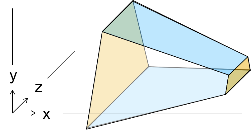
Figure 1: 3-d Trapezoidal Volume

We call this data structure a trapezoid because, for every dimension greater than one, the bounds on the variable of that dimension are, in general, linear relations expressed in terms of the preceding variable. Holding all other variables constant, such linear bounds describe trapezoidal regions; hence the name.

The data structure we use to represent generalizations is a region. A region is defined as either a trapezoid or the complement of a trapezoid:

$$R\equiv\{T\}\;|\;\,^{\sim}\{T\}$$

2 Generalization

An ACL2 proof that a low-level implementation of the following generalization procedure satisfies our notion of generalization correctness is provided in the supporting materials accompanying this paper. The following presentation provides an overview of the generalization process but limits discussion of correctness to observations concerning key steps in this proof along with references to the supporting materials.

2.1 Generalization Correctness

Given a formula $F$ and a consistent reference vector $\vec{v}=v_{\_}n,\ldots,v_{\_}1$, the objective is to compute a region $R$ which correctly generalizes $\vec{v}$ with respect to $F$. We say that a generalization is correct if it satisfies the following properties:

• Invariant 1$\ \ F[\vec{v}]=R[\vec{v}]$

• Invariant 2.a If $F[\vec{v}]$, then $\forall\vec{w}.~{}R[\vec{w}]\Rightarrow F[\vec{w}]$

• Invariant 2.b If not $F[\vec{v}]$, then $\forall\vec{w}.~{}F[\vec{w}]\Rightarrow R[\vec{w}]$

The first invariant ensures that the reference vector is contained in the generalization iff the vector satisfies the original formula. The second two invariants ensure that the generalized result is a conservative under-approximation of the original formula. Together they guarantee that the state space that contains the reference vector in the generalized result is a subset of the state space that contains the reference vector in the original formula.

2.2 Generalization Process

The generalization process involves transforming a reference vector and a logical formula into a trapezoidal region. Generalizing relative to linear formula (Section 2.6) begins by transforming linear relations into regions (Section 2.3) and it proceeds by alternately intersecting and complementing the resulting regions (Section 2.5). The process of intersecting regions may further involve generalizing the intersection of sets of linear bounds into trapezoids (Section 2.4). The rules for each of these operations is presented in a bottom-up fashion.

2.3 Generalizing Linear Relations

We use $\left\langle{\left\langle{L}\right\rangle}\right\rangle\overset{\vec{v}}{\longrightarrow}R$ to represent the generalization of a linear relation ($L$) into a trapezoidal region ($R$), a process which may involve several steps. First, arbitrary linear relations between two polynomials can be expressed as linear relations between a polynomial and zero.

$$\left\langle{\left\langle{P_{\_}i\prec P_{\_}j}\right\rangle}\right\rangle\overset{\vec{v}}{\longrightarrow}\left\langle{\left\langle{P_{\_}i-P_{\_}j\prec 0}\right\rangle}\right\rangle\hskip 8.0pt\left\langle{\left\langle{P_{\_}i\succ P_{\_}j}\right\rangle}\right\rangle\overset{\vec{v}}{\longrightarrow}\left\langle{\left\langle{P_{\_}j-P_{\_}i\prec 0}\right\rangle}\right\rangle\hskip 8.0pt\left\langle{\left\langle{P_{\_}i=P_{\_}j}\right\rangle}\right\rangle\overset{\vec{v}}{\longrightarrow}\left\langle{\left\langle{P_{\_}i-P_{\_}j=0}\right\rangle}\right\rangle$$

Constant linear relations normalize into either the true (empty) trapezoid or its complement.

$$\left\langle{\left\langle{c_{\_}0\prec 0}\right\rangle}\right\rangle \overset{\vec{v}}{\longrightarrow}\ \{\}\hskip 10.0pt\mbox{if $c_{\_}0\prec 0$}\hskip 55.0pt\left\langle{\left\langle{c_{\_}0=0}\right\rangle}\right\rangle\overset{\vec{v}}{\longrightarrow}\ \{\}\hskip 10.0pt\mbox{if $c_{\_}0=0$}$$

$$\left\langle{\left\langle{c_{\_}0\prec 0}\right\rangle}\right\rangle \overset{\vec{v}}{\longrightarrow}\,^{\sim}\{\}\hskip 10.0pt\mbox{if $\,{}^{\lnot}(c_{\_}0\prec 0)$}\hskip 35.0pt\left\langle{\left\langle{c_{\_}0=0}\right\rangle}\right\rangle\overset{\vec{v}}{\longrightarrow}\,^{\sim}\{\}\hskip 10.0pt\mbox{if $\,{}^{\lnot}(c_{\_}0=0)$}$$

Non-constant linear relations between polynomials and zero are normalized so that they relate the variable with the largest dimension to a polynomial consisting only of smaller variables and constants.

$$\left\langle{\left\langle{P_{\_}n<0}\right\rangle}\right\rangle \overset{\vec{v}}{\longrightarrow}\left\langle{\left\langle{x_{\_}n<-(P_{\_}n/c_{\_}n-x_{\_}n)}\right\rangle}\right\rangle\hskip 35.0pt\mbox{if $c_{\_}n>0$}$$

$$\left\langle{\left\langle{P_{\_}n<0}\right\rangle}\right\rangle \overset{\vec{v}}{\longrightarrow}\left\langle{\left\langle{-(P_{\_}n/c_{\_}n-x_{\_}n)<x_{\_}n}\right\rangle}\right\rangle\hskip 35.0pt\mbox{if $c_{\_}n<0$}$$

$$\left\langle{\left\langle{P_{\_}n\leq 0}\right\rangle}\right\rangle \overset{\vec{v}}{\longrightarrow}\left\langle{\left\langle{x_{\_}n\leq-(P_{\_}n/c_{\_}n-x_{\_}n)}\right\rangle}\right\rangle\hskip 35.0pt\mbox{if $c_{\_}n>0$}$$

$$\left\langle{\left\langle{P_{\_}n\leq 0}\right\rangle}\right\rangle \overset{\vec{v}}{\longrightarrow}\left\langle{\left\langle{-(P_{\_}n/c_{\_}n-x_{\_}n)\leq x_{\_}n}\right\rangle}\right\rangle\hskip 35.0pt\mbox{if $c_{\_}n<0$}$$

$$\left\langle{\left\langle{P_{\_}n=0}\right\rangle}\right\rangle \overset{\vec{v}}{\longrightarrow}\left\langle{\left\langle{x_{\_}n=-(P_{\_}n/c_{\_}n-x_{\_}n)}\right\rangle}\right\rangle\hskip 35.0pt\mbox{}$$

Normalized linear relations that are true at the reference vector simply become singleton trapezoidal regions.

$$\left\langle{\left\langle{x_{\_}n\prec P}\right\rangle}\right\rangle\overset{\vec{v}}{\longrightarrow}\{(x_{\_}n\prec P)\}\hskip 35.0pt\mbox{if $x_{\_}n[\vec{v}]\prec P[\vec{v}]$}$$

$$\left\langle{\left\langle{P\prec x_{\_}n}\right\rangle}\right\rangle\overset{\vec{v}}{\longrightarrow}\{(P\prec x_{\_}n)\}\hskip 35.0pt\mbox{if $P[\vec{v}]\prec x_{\_}n[\vec{v}]$}$$

$$\left\langle{\left\langle{x_{\_}n=P}\right\rangle}\right\rangle\overset{\vec{v}}{\longrightarrow}\{(x_{\_}n=P)\}\hskip 35.0pt\mbox{if $x_{\_}n[\vec{v}]=P[\vec{v}]$}$$

A normalized linear relation that evaluates to false at the reference vector, however, is expressed as a negated trapezoidal region containing a single linear relation that is true at the reference vector.

$$\left\langle{\left\langle{x_{\_}n<P}\right\rangle}\right\rangle \overset{\vec{v}}{\longrightarrow}\,^{\sim}\{(P\leq x_{\_}n)\}\hskip 35.0pt\mbox{if $\,{}^{\lnot}(x_{\_}n[\vec{v}]<P[\vec{v}])$}$$

$$\left\langle{\left\langle{x_{\_}n\leq P}\right\rangle}\right\rangle \overset{\vec{v}}{\longrightarrow}\,^{\sim}\{(P<x_{\_}n)\}\hskip 35.0pt\mbox{if $\,{}^{\lnot}(x_{\_}n[\vec{v}]\leq P[\vec{v}])$}$$

$$\left\langle{\left\langle{P<x_{\_}n}\right\rangle}\right\rangle \overset{\vec{v}}{\longrightarrow}\,^{\sim}\{(x_{\_}n\leq P)\}\hskip 35.0pt\mbox{if $\,{}^{\lnot}(x_{\_}n[\vec{v}]>P[\vec{v}])$}$$

$$\left\langle{\left\langle{P\leq x_{\_}n}\right\rangle}\right\rangle \overset{\vec{v}}{\longrightarrow}\,^{\sim}\{(x_{\_}n<P)\}\hskip 35.0pt\mbox{if $\,{}^{\lnot}(x_{\_}n[\vec{v}]\geq P[\vec{v}])$}$$

$$\left\langle{\left\langle{x_{\_}n=P}\right\rangle}\right\rangle \overset{\vec{v}}{\longrightarrow}\,^{\sim}\{(P<x_{\_}n)\}\hskip 35.0pt\mbox{if $(x_{\_}n[\vec{v}]>P[\vec{v}])$}$$ (neq.1)

$$\left\langle{\left\langle{x_{\_}n=P}\right\rangle}\right\rangle \overset{\vec{v}}{\longrightarrow}\,^{\sim}\{(x_{\_}n<P)\}\hskip 35.0pt\mbox{if $(x_{\_}n[\vec{v}]<P[\vec{v}])$}$$ (neq.2)

Normalizing linear relations in this way ensures that every variable bound contained in the body of a trapezoid is true at the reference vector. It also ensures that regions that contain the reference vector simplify into simple trapezoids while those that do not are expressed as the complement of a trapezoid that does.

With the exception of rules neq.1 and neq.2, the rules for generalizing linear relations ensure that the generalization is equal to the original formula (i.e. $\forall w.~{}F[\vec{w}]=L[\vec{w}]$), trivially satisfying our correctness invariants. Crucially, rules neq.1 and neq.2 do satisfy Invariants 1 and 2.b (and, trivially, 2.a) as expressed in Section 2.1, ensuring that, in all cases, our generalization of linear constraints is correct. See the functions normalize-equal-0 and normalize-gt-0 and their associated lemmas in the file top.lisp of the supporting materials.

2.4 Generalizing Bound Intersections

Let $C$ be a set of normalized bounds known to be satisfiable as witnessed by the consistent reference vector $\vec{v}$. The relation $C\mathrel{\overset{\vec{v}}{\longrightarrow}\!\!{}^{*}}T$ represents the fixed-point of intersecting and reducing the various bounds contained in $C$ into a trapezoidal region. The following collection of rules govern the individual intersections of the members of such a set of bounds to produce a trapezoid. The rules of the rewrite system operate on an un-ordered set of bounds, allowing for arbitrary reordering of the bounds. The key to this process are rules for eliminating multiple bounds on the same variable. The rules for eliminating multiple upper bounds are shown below. The rules for multiple lower bounds are symmetric.

$$(x_{\_}n<P)\cap(x_{\_}n<Q)\overset{\vec{v}}{\longrightarrow}(x_{\_}n<P)\cap\left\langle{\left\langle{P\leq Q}\right\rangle}\right\rangle\hskip 35.0pt\mbox{if $P[\vec{v}]\leq Q[\vec{v}]$}$$ (lt-int.1)

$$(x_{\_}n<P)\cap(x_{\_}n\leq Q)\overset{\vec{v}}{\longrightarrow}(x_{\_}n<P)\cap\left\langle{\left\langle{P\leq Q}\right\rangle}\right\rangle\hskip 35.0pt\mbox{if $P[\vec{v}]\leq Q[\vec{v}]$}$$ (lt-int.2)

$$(x_{\_}n\leq P)\cap(x_{\_}n<Q)\overset{\vec{v}}{\longrightarrow}(x_{\_}n\leq P)\cap\left\langle{\left\langle{P<Q}\right\rangle}\right\rangle\hskip 35.0pt\mbox{if $P[\vec{v}]<Q[\vec{v}]$}$$ (lt-int.3)

$$(x_{\_}n\leq P)\cap(x_{\_}n\leq Q)\overset{\vec{v}}{\longrightarrow}(x_{\_}n\leq P)\cap\left\langle{\left\langle{P\leq Q}\right\rangle}\right\rangle\hskip 35.0pt\mbox{if $P[\vec{v}]\leq Q[\vec{v}]$}$$ (lt-int.4)

Note that while $\left\langle{\left\langle{P\prec Q}\right\rangle}\right\rangle$ normalizes the linear relation as described in Section 2.3 this bound will never evaluate to false due to the rules’ side-conditions. Consequently the result will always be a simple trapezoid which is either empty (if both bounds are constant) or contains a single normalized bound on a variable whose dimension is less than that of $x_{\_}n$. Similar observations apply to the rules for simplifying bounds involving equality, as shown below. This process and it’s correctness is captured by the function andTrue-variableBound-variableBound and its associated lemmas (generated by the def::trueAnd macro) in the file poly-proofs.lisp of the supporting materials.

$$(x_{\_}n=P)\cap(x_{\_}n\prec Q)\overset{\vec{v}}{\longrightarrow}(x_{\_}n=P)\cap\left\langle{\left\langle{P\prec Q}\right\rangle}\right\rangle$$ (eq-int.1)

$$(x_{\_}n=P)\cap(Q\prec x_{\_}n)\overset{\vec{v}}{\longrightarrow}(x_{\_}n=P)\cap\left\langle{\left\langle{Q\prec P}\right\rangle}\right\rangle$$ (eq-int.2)

$$(x_{\_}n=P)\cap(x_{\_}n=Q)\overset{\vec{v}}{\longrightarrow}(x_{\_}n=P)\cap\left\langle{\left\langle{P=Q}\right\rangle}\right\rangle$$ (eq-int.3)

Lemma 2.1.

The intersection rules are terminating.

Proof.

Define a measure on the conjunction of bounds to be the sum of the dimension of each bound. Each rule of the intersection rewrite system reduces this measure. For example, consider rule lt-int.1. We know $dim(x)>dim(P)$ and $dim(x)>dim(Q)$, and thus $dim(x)>dim(\langle P\leq Q\rangle)$ and in particular $dim(x<Q)>dim(\langle P\leq Q\rangle)$. Since the measure is always non-negative, the intersection rules are terminating. See the def::total event for the function intersect in the file intersection.lisp of the supporting materials for a proof of termination for ordered (not un-ordered, see Section 3.0.1) bounds. ∎

Lemma 2.2.

When run to completion, the intersection rules result in a trapezoid.

Proof.

The intersection rules apply to a set of bounds that are normalized and satisfiable. To qualify as a trapezoid the only missing requirement is that there may be multiple upper, lower, and equality bounds on each variables. For multiple upper bounds, note that the 4 rules above cover all cases. Although rule lt-int.3 does not cover the case when $P[\vec{v}]=Q[\vec{v}]$, that case will in fact be covered by rule lt-int.2 since then $Q[\vec{v}]\leq P[\vec{v}]$. The case of multiple lower bounds is symmetric. Therefore, the rewrite rules will eliminate all multiple and lower and upper bounds so that the result is a trapezoid. See lemma trapezoid-p-intersect in the file intersection.lisp of the supporting materials. ∎

While, in general, the the fixed-point resulting from intersecting and reducing a set of bounds will differ from the original set, each rule that we apply to perform this normalization satisfies Invariants 1 and 2.a (and trivially 2.b) as expressed in Section 2.1, ensuring the correctness of this process.

2.5 Generalizing Region Intersections and Complements

The relation $R^{a}\cap R^{b}\overset{\vec{v}}{\rightarrowtail}R^{c}$ indicates that region $R^{c}$ is a generalized intersection of regions $R^{a}$ and $R^{b}$ relative to $\vec{v}$ and $\,{}^{\sim}R^{a}\overset{\vec{v}}{\rightarrowtail}R^{b}$ to indicate that $R^{b}$ is the generalized complement of $R^{a}$. We characterize the behavior of region intersection and complement with the following set of rules:

$$\,{}^{\sim}{\,{}^{\sim}{\{T\}}}\overset{\vec{v}}{\rightarrowtail}\{T\}\hskip 35.0pt\{T^{a}\}\cap\{T^{b}\}\overset{\vec{v}}{\rightarrowtail}\{T^{c}\}T^{a}\cap T^{b}\mathrel{\overset{\vec{v}}{\longrightarrow}\!\!{}^{*}}T^{c}$$

$$\,{}^{\sim}{\{T\}}\cap R\overset{\vec{v}}{\rightarrowtail}\,^{\sim}{\{T\}}\hskip 35.0ptR\cap\,^{\sim}{\{T\}}\overset{\vec{v}}{\rightarrowtail}\,^{\sim}{\{T\}}$$

While perhaps surprising, the rules cint.1 and cint.2 not only simplify the region intersection process, they are also both consistent with and essential for preserving generalization correctness (specifically, Invariant 2.b) as described in Section 2.1. See the functions and-regions and not-region and their associated lemmas in the file top.lisp from the supporting materials.

2.6 Generalizing Linear Formulae

We write $F\overset{\vec{v}}{\Rightarrow}R$ to mean that region $R$ generalizes $\vec{v}$ with respect to formula $F$. In general, conjunction generalizes into region intersection, negation generalizes into region complement, and disjunction generalizes into a complement of the intersection of the complements of the generalized arguments. The generalization relation is defined inductively over the structure of the formula $F$.

$$L\overset{\vec{v}}{\Rightarrow}R\left\langle{\left\langle{L}\right\rangle}\right\rangle\overset{\vec{v}}{\longrightarrow}R\hskip 35.0ptF_{\_}1\land F_{\_}2\overset{\vec{v}}{\Rightarrow}R_{\_}1\cap R_{\_}2\lx@proof@logical@and F_{\_}1\overset{\vec{v}}{\Rightarrow}R_{\_}1F_{\_}2\overset{\vec{v}}{\Rightarrow}R_{\_}2$$

$$\,{}^{\lnot}F\overset{\vec{v}}{\Rightarrow}\,^{\sim}RF\overset{\vec{v}}{\Rightarrow}R\hskip 35.0ptF_{\_}1\lor F_{\_}2\overset{\vec{v}}{\Rightarrow}\,^{\sim}(\,^{\sim}R_{\_}1\cap\,^{\sim}R_{\_}2)\lx@proof@logical@and F_{\_}1\overset{\vec{v}}{\Rightarrow}R_{\_}1F_{\_}2\overset{\vec{v}}{\Rightarrow}R_{\_}2$$

This procedure can be shown to satisfy our correctness invariants by induction over the structure of a linear formula and by appealing to the correctness of the generalization of linear relations and region intersection. See the definition generalize-ineq and the theorems inv1-generalize-ineq and inv2-generalize-ineq in the file top.lisp of the supporting materials.

3 Sampling

Sampling is the process of identifying randomized, concrete, type-consistent variable assignments (vectors) that satisfy all of the variable bounds in a trapezoid . We call this process sampling, rather than solving, to emphasize the fact that it is intended to be randomized, simple, and efficient. Indeed, the structure of a trapezoid lends itself to a simple and efficient sampling algorithm. The trapezoidal structure ensures that the variable with the smallest dimension is bounded only by constants. Sampling of the smallest dimension variable therefore involves simply choosing a value consistent with its type and constant bounds. Because each normalized variable bound is expressed strictly in terms of variables of smaller dimension, sampling the variables by proceeding from the smallest to the largest dimension guarantees that the bounds on each subsequent variable will evaluate to constants relative to variables already assigned. Sampling each variable from the smallest to the largest dimension, therefore, involves nothing more than choosing a value for each variable consistent with type and constant bounds computed based on the previous variable assignments.

While the above algorithm is certainly simple and efficient, the trapezoidal data structure as defined is not sufficient to guarantee that every variable assignment that satisfies the first $N$ bounds will satisfy the $N+1^{th}$ bound. A given set of variable assignments may result in an upper bound that is smaller than a lower bound or, more subtly, an integer variable may be constrained by bounds that do not permit an integral solution. While backtracking and attempting different sets of variable assignments is possible in such cases, it can also be very inefficient.

To address this concern we present an overview of a post-processing step for trapezoids, performed before sampling, that results in a restricted trapezoid with properties that ensure that the simple and efficient sampling algorithm presented above will never encounter a bound that cannot be satisfied (even for integer variables) and thus never needs to backtrack. While the following procedure has not been mechanically verified, we sketch selected aspects of the informal proof with the long term objective of formalizing and verifying its correctness in ACL2.

3.0.1 Ordered Trapezoids

To better explain our post-processing approach we first introduce a more refined representation for trapezoids, beginning with the concept of variable intervals. A variable interval is either a single variable bound or a pair of bounds consisting of an upper and lower bound on the same variable. The dimension of an interval is simply the dimension of the bound variable. Variable intervals allow us to gather all of the linear bounds relevant to each variable in one place.

$$I_{\_}n\equiv B_{\_}n\;|\;(P^{L}\prec x_{\_}n)\cap(x_{\_}n\prec P^{U})$$

Variable intervals can be used to construct ordered trapezoids. An ordered trapezoid is simply a sequence of variable intervals organized in descending order based on dimension, terminating in the empty trapezoid. Note that these new syntactic constructs do not change in any way the nature of trapezoids other than to impose additional ordering constraints on their representation.

$$T_{\_}n \equiv\ I_{\_}n\cap T_{\_}m\ \ \mbox{where $n>m$}$$

$$T_{\_}0 \equiv\varnothing$$

Using ordered trapezoids, we can define the process for sampling a trapezoid, $\epsilon(T)$ to produce a consistent vector that satisfies the trapezoid. Note that $\epsilon(I_{\_}n[\vec{w}])$ represents a random choice of a value consistent in type with variable $n$ and satisfying the interval $I_{\_}n$ evaluated at the vector $\vec{w}$ (assuming such a value exists), $\{\}$ represents an empty vector, and $\vec{w}[i]=x$ represents an update of vector $\vec{w}$ such that dimension $i$ is equal to the value $x$.

$$\epsilon(\varnothing)\rightarrow\{\}\hskip 35.0pt\epsilon(I_{\_}n\cap T_{\_}m)\rightarrow\vec{w}[n]=\epsilon(I_{\_}n[\vec{w}])\epsilon(T_{\_}m)\rightarrow\vec{w}$$

3.1 Restriction

The purpose of post-processing is to restrict the domain of values that can be assigned to selected variables in the trapezoid to ensure that the sampling process can proceed without backtracking. We call the trapezoidal post-processing step restriction. The restriction process takes as input a trapezoid, a change of basis ($\sigma$, initially an identity function), and a consistent reference vector. The output of the restriction process is a new (restricted) trapezoid and a change of basis that maps vectors sampled from the restricted trapezoid back into the vector space of the original trapezoid.

$$T,\,\sigma,\,\vec{v}\overset{\textit{R}}{\longrightarrow}T^{\prime},\,\sigma^{\prime}$$

The restriction process is specified as a single pass over the trapezoid intervals, starting with the largest interval and proceeding to the smallest. Each interval in the trapezoid is restricted by applying the steps summarized below.

• Bound Fixing (BF) Ensures that linear bounds are expressed only in terms of $\geq$ and $\leq$.

• Integer Equality (IE) Ensures that equalities involving integer variables are always satisfiable.

• Interval Restriction (IR) Ensures that intervals are always satisfiable.

Each interval in the trapezoid may suggest a domain restriction, in the form of a set of linear constraints, and a change of basis in the form of a linear transformation. Domain restrictions are intersected with the remaining trapezoid before it, too, is restricted. Changes of base are accumulated and applied to the current interval, the remaining trapezoid, and the reference vector. When complete, the final restricted trapezoid and the final change of basis are returned.

$$\varnothing,\,\sigma,\,\vec{v}\overset{\textit{R}}{\longrightarrow}\varnothing,\,\sigma$$

Therestrictedtrapezoidcanth