Detection and Mitigation of Biasing Attacks on Distributed Estimation Networks

Abstract

The paper considers a problem of detecting and mitigating biasing attacks on networks of state observers targeting cooperative state estimation algorithms. The problem is cast within the recently developed framework of distributed estimation utilizing the vector dissipativity approach. The paper shows that a network of distributed observers can be endowed with an additional attack detection layer capable of detecting biasing attacks and correcting their effect on estimates produced by the network. An example is provided to illustrate the performance of the proposed distributed attack detector.

1 Introduction

Recent developments in the area of networked control and estimation have been increasingly focused on resilience of networked control systems to intentional malicious input attacks aiming to compromise stability and performance of control systems. Owing to the networked nature of such control systems, typically not all measurements are available at nodes of the network to allow efficient attack and fault detection [7, 21]; this has made distributed approaches particularly attractive. For instance, [25] considers distributed fault detection for second order dynamics at each node. Each node has the model of the entire network or the model of its neighbourhood; in the latter case interconnections of the neighbours to the agents outside the neighbourhood are treated as undesirable disturbances to be rejected. A bank of fault observers is constructed for each fault model. The situation is considered where the network topology is uncertain, and can be captured as a norm-bounded uncertain perturbation of the global network model.

Another fault detection algorithm is proposed in [10] which considers a fault input to the plant with multiple randomly failing sensors (random packet drop-out) for a discrete-time system. A discrete-time system model is also considered in [8], and it is assumed that both plant and sensors are subject to Markovian switching. The reference considers a fault input to the plant and uses sensor information fusion from several nodes to generate the residuals for fault detection.

A considerable progress on the problem has been achieved in [20] which not only considered the problem of residual generation for linear systems given in a quite general descriptor form, but also has characterized system vulnerabilities from the system theoretic perspective of attack input detectability. We also refer to [21] where connections have been drawn between the network topology and attack input detectability.

This paper considers the problem of detecting attacks on consensus-based distributed estimation networks. The topic of distributed estimation has gained considerable attention in the literature, in a bid to reduce communication bottlenecks and improve reliability and fidelity of centralized state observers. Filter cooperation and consensus ideas have proved to be instrumental in the design of distributed state observers [17, 24, 27]. At the same time, consensus-based systems are particularly vulnerable to intentional attacks since the compromised agents can interfere with the functions of the entire network in a significant way [19]. Uncertainty and noise represent another challenge from the attack detection viewpoint — state observers are typically required in applications where uncertainty and noise make accessing the system state difficult; this may allow the attackers to remain undetected by injecting signals compatible with the noise statistics [20]. This motivates an increased interest in detection of rogue behaviours of state observers [14].

In this paper, we are concerned with resilience properties of a general class of distributed state estimation networks considered, for example, in [24, 27, 29]. The attack model assumes that the state observers at the compromised nodes are driven by certain attack/fault inputs. Referring to conventional false-data injection models [26], the model considered here is quite general, with several noteworthy features. Firstly, we consider the attacks that force a rogue behaviour at the affected node by interfering with the data processing algorithm. Similar to bias injection attacks considered in [26], the attack inputs are not assumed to be constant and can include an uncertain transient component to reflect the adversary’s desire to make the attack stealthy. The purpose of the attack under consideration is to force the compromised node to produce biased state estimates and then exploit interconnections within the network to propagate those estimates across the network.

In terms of resources required to launch an attack, the adversary does not require any knowledge of the system model to carry out the attack, it relies on the misappropriated observer to produce rogue messages which are then injected into other nodes of the network through existing network communications. Our interest in this paper is in detecting and tracking attack/fault inputs causing such a rogue behaviour. For this, the paper proposes to introduce additional filters in the attack detectors at every network node. The idea behind the introduction of such filters is to differentiate imminently dangerous components of the attack inputs from components whose effect is akin to that of ‘ever-present disturbances’. Since distributed $H_{\infty}$ observers such as those considered in [24, 27, 29] are constructed to attenuate disturbances, by design they are less sensitive to exogenous ‘disturbance-like’ inputs. On the other hand, low-frequency biasing inputs such as constant inputs do not directly fit within the class of ‘finite-energy disturbances’ typically considered within the $H_{\infty}$ design. Such inputs may cause node observers to produce biased state estimates, therefore they are of primary concern. The proposed filters are to assist with monitoring the node observers to detect biases caused by such inputs.

Tracking disturbances in a large-scale system is not uncommon. E.g., in [23] distributed integral action controllers were used for averaging constant disturbances to enable all agents in the system to synchronize to a common reference system governed by the averaged constant disturbance. In contrast, in this paper we aim at tracking and suppressing individual attack inputs applied at certain observer nodes, rather than tracking an averaged attack vector. Additional filter dynamics introduced in the fault detectors are instrumental to solve that task.

From the viewpoint of fault detection/input estimation, the system subject to attack is distributed itself. This problem setting is similar to [25], but is different from [10, 8] which were focused on detecting faults in the plant. Overall, the techniques developed in this paper have a number of distinct features:

1. We are concerned with resilience of general multidimensional consensus-based observers to biasing attacks that target estimation algorithms at misappropriated observer nodes rather than sensor measurements or communication channels.

2. The proposed attack detector is distributed and the node detectors interact to detect and mitigate the attack.

3. Our approach utilizes methodologies of vector dissipativity and $H_{\infty}$ estimation. This allows us to accommodate uncertainties in the sensors and the plant model.

4. The proposed attack detectors utilize the same plant measurements and the same communication channels that are used by the networked observer to solve the original plant estimation task. But extra information needs to be communicated between the neighbour agents. This allows us to determine which of the node observers is compromised, without introducing additional communication sensors or communication channels.

The paper is an extended version of the conference paper [5]. Compared with the conference version, the paper has been substantially extended. The present version includes complete proofs and an example which were not included in the preliminary version. The presentation has been substantially revised, to show that the results hold under somewhat less restrictive design conditions. Also, two new sections have been added which discuss the detectability conditions of the network and show that the proposed attack detectors can be used for countering biasing attacks on a network of distributed observers under consideration, providing the distributed estimation algorithms under consideration with an additional level of resilience.

The paper is organised as follows. In Section 2, a background on distributed consensus based estimation is presented, and the model of attack is introduced. The class of biasing attacks is formally defined in Section 3, and the attack detection problem is also formulated in that section. The main results are given in Section 4, where sufficient conditions in terms of coupled linear matrix inequalities are expressed to enable the design of a networked attack detector. In Section 5, we show that the outputs of the proposed attack detectors can be used for correcting biased state estimates. This allows the system to remain operational under attack, meeting the objective of resilient system design. Conditions on detectability of the network are discussed in Section 6. An illustrative example is presented in Section 7, and finally some concluding remarks are given in Section 8.

Notation: $\mathbf{R}^{n}$ denotes the real Euclidean $n$-dimensional vector space, with the norm $\|x\|=(x^{\prime}x)^{1/2}$; here the symbol ^′ denotes the transpose of a matrix or a vector. The symbol $I$ denotes the identity matrix, and $0_{m\times n}$ denotes the zero matrix of size $m\times n$. We will occasionally use $I$ and $0$ for notational convenience if no confusion is expected. The symbols $|\cdot|$ and $\mathrm{Re}(\cdot)$ denote respectively the magnitude and the real part of a complex number. For real symmetric $n\times n$ matrices $X$ and $Y$, $Y>X$ (respectively, $Y\geq X$) means the matrix $Y-X$ is positive definite (respectively, positive semidefinite). $\mathrm{Ker}$ and $\mathrm{rank}$ denote the null-space and rank of a matrix. The notation $L_{2}[0,\infty)$ refers to the Lebesgue space of $\mathbf{R}^{n}$-valued vector-functions $z(.)$, defined on the time interval $[0,\infty)$, with the norm $\|z\|_{2}\triangleq\left(\int_{0}^{\infty}\|z(t)\|^{2}dt\right)^{1/2}$ and the inner product $\int_{0}^{\infty}z_{1}^{\prime}(t)z_{2}(t)dt$.

2 Background: Continuous-time distributed estimation

Consider an observer network with $N$ nodes and a directed graph topology $\mathbf{G}=(\mathbf{V},\mathbf{E})$ where $\mathbf{V}$ and $\mathbf{E}$ are the set of vertices and the set of edges (i.e, the subset of the set $\mathbf{V}\times\mathbf{V}$), respectively. Without loss of generality, we let $\mathbf{V}=\{1,2,\ldots,N\}$. The graph $\mathbf{G}$ is assumed to be directed, reflecting the fact that while node $i$ receives the information from node $j$, this relation may not be reciprocal. The notation $(j,i)$ denotes the edge of $\mathbf{G}$ originating at node $j$ and ending at node $i$. It is assumed that the nodes of the graph $\mathbf{G}$ have no self-loops, i.e., $(i,i)\not\in\mathbf{E}$.

For each $i\in\mathbf{V}$, let $\mathbf{V}_{i}=\{j:(j,i)\in\mathbf{E}\}$ be the set of nodes supplying information to node $i$. The cardinality of $\mathbf{V}_{i}$, known as the in-degree of node $i$, is denoted $p_{i}$; i.e., $p_{i}$ is equal to the number of incoming edges for node $i$. Also, $q_{i}$ will denote the number of outgoing edges for node $i$, known as the out-degree of node $i$. Let $\mathbf{A}=[\mathbf{a}_{ij}]$ be the adjacency matrix of the digraph $\mathbf{G}$, i.e., $\mathbf{a}_{ij}=1$ if $(j,i)\in\mathbf{E}$, otherwise $\mathbf{a}_{ij}=0$. Then, $p_{i}=\sum_{j=1}^{N}\mathbf{a}_{ij}=\sum_{j\in\mathbf{V}_{i}}\mathbf{a}_{ij}$, $q_{i}=\sum_{j=1}^{N}\mathbf{a}_{ji}$.

A typical distributed estimation problem considers a plant described by the equation

$$\dot{x}=Ax+B\xi(t),\quad x(0)=x_{0},\quad x\in\mathbf{R}^{n},$$ (1)

governed by a disturbance input $\xi\in\mathbf{R}^{m}$. A network of filters connected according to the graph $\mathbf{G}$ takes measurements of the plant with the purpose to produce an estimate of $x$. It is assumed that each filter takes measurements

$$y_{i}=C_{i}x+D_{i}\xi+{\bar{D}_{i}}\xi_{i},$$ (2)

where $\xi_{i}(t)\in\mathbf{R}^{m_{i}}$ represents the measurement disturbance at the local sensing node $i$, and processes them locally using an information communicated by its neighbours $j$, $j\in\mathbf{V}_{i}$. An underlying feature of the problem is that in general, the pairs $(A,C_{i})$ are not required to be detectable. This has an implication that the nodes with undetectable pairs $(A,C_{i})$ can only obtain biased estimates of the plant, making cooperation between the nodes a necessity. Requirements on local sensors and the network to enable unbiased cooperative networked state estimation have been considered in the recent literature; e.g., see [6, 32, 2].

Depending on the nature of the disturbances $\xi$, $\xi_{i}$, cooperative processing of measurements can be done using Kalman [17], $H_{\infty}$ [24, 27, 29] filters, etc. Many of the existing algorithms utilize networks of cooperating filters, each producing an estimate $\hat{x}_{i}$ of the state $x$ using an observer of the form

$$\dot{\hat{x}}_{i}=A\hat{x}_{i}+L_{i}(y_{i}(t)-C_{i}\hat{x}_{i})+K_{i}\sum_{j\in\mathbf{V}_{i}}H(\hat{x}_{j}-\hat{x}_{i}),$$ (3)

$$\hat{x}_{i}(0)=0;$$

here the matrices $L_{i}$, $K_{i}$ are the parameters of the filter. Each filter combines processing of innovations obtained from local measurements with feedback from its neighbours, captured in the last term (3) where the neighbours’ estimates are $\hat{x}_{j}$, $j\in\mathbf{V}_{i}$. The matrix $H$ determines what information about $\hat{x}_{j}$ is shared between the nodes. For simplicity of presentation, we assume that communication channels between the nodes are ideal, and node $i$ receives the precise value of $H\hat{x}_{j}$, and that the matrices $H$ are identical across the network. More general formulations which allow for disturbances in communication channels and heterogeneity in communicated information can be easily accommodated within our approach, as they do not bring additional technical challenges.

The general problem of distributed estimation is to determine estimator gains $L_{i}$ and $K_{i}$ in (3) to ensure the filter internal stability and acceptable filtering performance against disturbances. Therefore, from the system resilience viewpoint it is of interest to consider the situation where one or several nodes of the network of observers (3) are subject to an attack whose aim is to interfere with these filtering performance objectives. A most common scenario of such an attack considered in the literature involves the attacker tempering with the measurements and/or communications between the nodes. In contrast, we consider the situation where the attacker mounts an attack on the observer dynamics directly. That is, we consider the scenario where some of the nodes are misappropriated by the attacker and, in lieu of (3), generate their estimates according to

$$\dot{\hat{x}}_{i} = A\hat{x}_{i}+L_{i}(y_{i}(t)-C_{i}\hat{x}_{i})$$ (4)

$$+K_{i}\sum_{j\in\mathbf{V}_{i}}H(\hat{x}_{j}-\hat{x}_{i})+F_{i}f_{i},\qquad\hat{x}_{i}(0)=0.$$

Here $F_{i}\in\mathbf{R}^{n\times n_{f}}$ is a constant “fault entry matrix” (e.g., see [22]) and $f_{i}\in\mathbf{R}^{n_{f}}$ is the unknown signal representing an attack input. The gains of the observers and the network topology are not affected by the attacker and are assumed to be fixed (cf. [6]). From now on, our focus is exclusively on the network of observers (4), although our approach to detection and mitigation of biasing attacks can be readily applied to other mentioned distributed state estimation algorithms as well. For instance, if the communication link between node $i$ and $k:k\in\mathbf{V}_{i}$ is under attack such that node $k$ instead of receiving $\hat{x}_{k}$ receives a biased estimate of $\hat{x}_{k}+\ell_{ik}$ where $\ell_{ik}$ is an attack signal, then this situation is still captured by the biased estimator model (4) in which $F_{i}=K_{i}H$ and $f_{i}=\ell_{ik}$. Therefore, the analysis presented in the paper is applicable to this type of attack as well.

The class of attacks considered in this paper does not contain attacks that cause nodes or links to fall out of the network. Our consideration is that the objectives of the biasing attacker are different from the objectives of a jamming attacker. Attacking links to fail is a kind of DoS attack, and these attacks disrupt the normal flow of information within the network. In contrast, the biasing attacker who misappropriates a node benefits from integrity of the network links, since it uses them to spread the biased $\hat{x}_{i}$ across the network. Therefore the analysis in the paper is carried out under the assumption that it is not in the attacker’s interests to block network links. Attack stealthiness considerations also support this assumption. While jammers act openly to block communication links or sensing nodes, we consider that the intention of a biasing attacker is to remain hidden, in order to inject the false data for as long as possible. Unusual patterns in nodes and links failures will likely to prompt maintenance which may reveal the attacker. Thus it may be risky for the biasing attacker to disrupt connectivity if it wishes to remain stealthy.

\psfrag{R}{$f_{i}$}\psfrag{nu}{$-\nu_{i}$}\psfrag{Y}{$\hat{f}_{i}$}\psfrag{H}{$G_{i}(s)$}\psfrag{G}{$\frac{1}{s}$}\psfrag{+}{$+$}\psfrag{-}{$-$}\includegraphics[width=195.12767pt]{Q2.eps}

Figure 1: An auxiliary ‘input tracking’ model.

3 Problem formulation

To be concrete, from now on we build the presentation around the distributed $H_{\infty}$ cooperative estimation problem [27, 29], although the approach to bias attack detection proposed in this paper is general enough to allow extensions to other types of filters in an obvious manner. In line with the disturbance model considered in [27, 29], it will be assumed throughout the paper that the disturbances $\xi$, $\xi_{i}$ belong to $L_{2}[0,\infty)$. This assumption suffices to guarantee that equation (1) has an $L_{2}$-integrable solution on any finite time interval $[0,T]$, even when the matrix $A$ is unstable.

3.1 Admissible biasing attacks

We now present a class of biasing attacks on misappropriated nodes of the filter (4) that will be considered in this paper. First consider a class of attack input signals $f_{i}(t)$, $t\geq 0$, of the form

$$f_{i}(t)=f_{i1}(t)+f_{i2}(t),$$ (5)

where the Laplace transform of $f_{i1}(t)$, $f_{i1}(s)$, is such that $f_{i1}^{\infty}\triangleq\sup_{\omega}\|\omega f_{i1}(j\omega)\|^{2}<\infty$ and $f_{i2}\in L_{2}[0,\infty)$. In particular, this class includes attack inputs whose Laplace transform is rational and has no more than one pole at the origin, with the remaining poles located in the open left half-plane of the complex plane. This class of inputs will be denoted $\mathscr{F}$. It includes as a special case bias injection attack inputs consisting of a steady-state component and an exponentially decaying transient component generated by a low pass filter introduced in [26].

It is easy to show that there exists a proper square $n_{f}\times n_{f}$ transfer function $G_{i}(s)$ for which the system in Fig. 1 is stable and

$$\int_{0}^{\infty}\|f_{i}-\hat{f}_{i}\|^{2}dt<\infty$$ (6)

for all $f_{i}$ with the properties stated above. Indeed, we can select $G_{i}(s)=\frac{N(s)}{D(s)}I$, for which the system in Fig. 1 is stable; here $N(s)$ and $D(s)$ are real polynomials with $\mathrm{deg}(N)\leq\mathrm{deg}(D)$. It follows from stability of the system in Fig. 1 that $j\omega D(j\omega)+N(j\omega)\neq 0$ $\forall\omega$. This conclusion trivially follows from the Nyquist criterion. Hence, $a\triangleq\sup_{\omega}\left|\frac{j\omega D(j\omega)}{j\omega D(j\omega)+N(j\omega)}\right|^{2}<\infty$. Then

$$\frac{1}{2\pi}\int_{-\infty}^{+\infty}\|(I+\frac{1}{j\omega}G_{i}(j\omega))^{-1}f_{i}(j\omega)\|^{2}d\omega$$

$$\leq f_{i1}^{\infty}\int_{-\infty}^{\infty}\left|\frac{D(j\omega)}{j\omega D(j\omega)+N(j\omega)}\right|^{2}d\omega$$

$$+a\int_{-\infty}^{\infty}\|f_{i2}(j\omega)\|^{2}d\omega<\infty.$$ (7)

Define $\nu_{i}=\hat{f}_{i}-f_{i}$. Denoting the Laplace transforms of $f_{i}$ and $\nu_{i}$ as $f_{i}(s)$ and $\nu_{i}(s)$ respectively, and noting that

$$\nu_{i}(s)=-(I+\frac{1}{s}G_{i}(s))^{-1}f_{i}(s),$$

we conclude from (7) that (6) is satisfied.

Furthermore, if $G_{i}(s)$ is selected so that

$$\lim_{s\to 0}\|(I+\frac{1}{s}G_{i}(s))^{-1}\|=0,$$ (8)

then for all inputs $f_{i}\in\mathscr{F}$,

$$\lim_{t\to\infty}\|f_{i}(t)-\hat{f}_{i}(t)\|=0.$$ (9)

The proof of this fact is given in the Appendix.

In summary, we have observed that a large class of biasing inputs (which includes bias injection attack inputs introduced in [26]) can be represented as

$$f_{i}=\hat{f}_{i}-\nu_{i},$$

where $\nu_{i}$ is an $L_{2}$ integrable discrepancy between the attack input $f_{i}$ and its ‘model’ $\hat{f}_{i}$. For this, the model generating transfer function $G_{i}(s)$ needs to satisfy very mild assumptions - it must be proper, and the closed loop system in Fig. 1 must be stable. Other than that, $G_{i}(s)$ can be chosen arbitrarily. This allows us to proceed assuming formally that a collection of transfer functions $G_{i}(s)$, $i=1,\ldots,N$, with the above properties has been selected, and a set of biasing inputs $f_{i}$ is associated with this selection of transfer functions consisting of all signals $f_{i}$ for which (6) holds. We will refer to the inputs from this set as admissible biasing inputs. Clearly, such set is quite rich; as we have shown, it subsumes all inputs (5) and, consequently, the input set $\mathscr{F}$ and biasing attack inputs defined in [26]. In addition, $L_{2}$-integrable inputs $f_{i}$ which represent attack inputs with a limited energy resource [26] also belong to the set of admissible inputs since they are trivially represented in the form (5). It must be stressed that even though $G_{i}(s)$ is selected, the details of admissible biasing inputs, e.g., the asymptotic steady-state value or the shape of the transient, remain unknown to the designer.

We conclude this section by presenting a state space form of the system in Fig. 1 which will be used in the sequel. Since $G_{i}(s)$ is proper, the transfer function $\frac{1}{s}G_{i}(s)$ is strictly proper. Hence, a state space realization for the system in Fig. 1, e.g., the minimal state space realization, is of the form

$$\dot{\epsilon}_{i}=\Omega_{i}\epsilon_{i}+\Gamma_{i}\nu_{i},\qquad\epsilon_{i}(0)=0,$$ (10)

$$\hat{f}_{i}=\Upsilon_{i}\epsilon_{i},$$

where $\nu_{i}=\hat{f}_{i}-f_{i}$ is an $L_{2}$-integrable input. For example, for the system $G_{i}(s)=\frac{d_{i}}{s+2\beta_{i}}I$, we can let $\epsilon_{i}\in\mathbf{R}^{2n_{f}}$, and

$$\Omega_{i}=\left[\begin{array}[]{cc}0&I\\ 0&-2\beta_{i}I\end{array}\right],\quad\Gamma_{i}=\left[\begin{array}[]{c}0\\ -d_{i}I\end{array}\right],\quad\Upsilon_{i}=[I~{}0].$$ (11)

In what follows, the state space model (10) will be used in the derivation of attack detectors, and the sufficient conditions for attack detection proposed in the paper will include the parameters of the model (10). Some trials may be required in order to select these parameters to obtain satisfactorily performing detectors.

3.2 The distributed attack detector

The objective of the paper is to design a distributed attack detection system which is capable of tracking and suppressing admissible attack inputs. To achieve this task, we first summarize the information about the network available at each node, which will be used by the attack detectors. This information consists of the pair of innovation output signals

$$\zeta_{i} = y_{i}-C_{i}\hat{x}_{i}=C_{i}(x-\hat{x}_{i})+D_{i}\xi+{\bar{D}_{i}}\xi_{i},$$ (12)

$$\bar{\zeta}_{i} = \sum_{j\in\mathbf{V}_{i}}H(\hat{x}_{j}-\hat{x}_{i}).$$ (13)

The idea behind introducing these outputs is as follows. If node $i$ is under attack, then its predicted sensor measurement $C_{i}\hat{x}_{i}$ is expected to be biased, compared to the actual measurement $y_{i}$. This must lead to a significant difference between these two signals, i.e., we must expect a large energy in $\zeta_{i}$. Likewise, the plant state estimate $\hat{x}_{i}$ at the misappropriated node $i$, is expected to deviate, at least during an initial stage of the attack, from the estimates produced at the neighbouring nodes. Thus, the variable $\bar{\zeta}_{i}$ describing dynamics of the disagreement between node $i$ and its neighbours is expected to differ from similar variables produced by network nodes not affected by the attack. This motivates using the innovation signals (12), (13) as inputs to the attack detector. They can be readily generated at node $i$; computing them only requires the local measurement $y_{i}$, the local estimate $H\hat{x}_{i}$ computed by the observer at node $i$ and the neighbours’ signals $H\hat{x}_{j}$, $j\in\mathbf{V}_{i}$, available at node $i$; see (4).

Let $e_{i}=x-\hat{x}_{i}$ be the local estimation error at node $i$. Using (1) and (4), it is straightforward to verify that each error $e_{i}$ satisfies the following equation:

$$\dot{e}_{i} = (A-L_{i}C_{i})e_{i}+K_{i}\sum_{j\in\mathbf{V}_{i}}H(e_{j}-e_{i})$$ (14)

$$+(B-L_{i}D_{i})\xi-L_{i}{\bar{D}_{i}}\xi_{i}-F_{i}f_{i},\quad e_{i}(0)=x_{0}.\qquad$$

Combine the system (14) with the auxiliary input tracking model (10):

$$\dot{e}_{i} = (A-L_{i}C_{i})e_{i}+K_{i}\sum_{j\in\mathbf{V}_{i}}H(e_{j}-e_{i})-F_{i}\Upsilon_{i}\epsilon_{i}$$

$$+ (B-L_{i}D_{i})\xi-L_{i}{\bar{D}_{i}}\xi_{i}+F_{i}\nu_{i},\quad e_{i}(0)=x_{0},$$

$$\dot{\epsilon}_{i} = \Omega_{i}\epsilon_{i}+\Gamma_{i}\nu_{i}\quad\epsilon_{i}(0)=0.$$ (15)

Here, we have used the relation $f_{i}=\Upsilon_{i}\epsilon_{i}-\nu_{i}$; see (10). The resulting system (15) equipped with the outputs (16), (17) can be regarded as an uncertain system governed by $L_{2}$-integrable inputs $\xi$, $\xi_{i}$ and $\nu_{i}$. Each such system is interconnected with its neighbours via inputs $e_{j}$, and the collection of all such systems represents a large-scale system. The innovations (12), (13) can be regarded as outputs of this large-scale system since they can be written in terms of the estimation errors as

$$\zeta_{i} = C_{i}e_{i}+D_{i}\xi+{\bar{D}_{i}}\xi_{i},$$ (16)

$$\bar{\zeta}_{i} = -\sum_{j\in\mathbf{V}_{i}}H(e_{j}-e_{i}).$$ (17)

We propose the following distributed $H_{\infty}$ observer for the large-scale system (15) as an attack detector for the observer network (4). The detector is to utilize the outputs (12), (13) of the system (4) (equivalently, the outputs (16), (17)) to estimate dynamics $e_{i}$ and $\epsilon_{i}$ of the system (15) while attenuating the disturbances $\xi$, $\xi_{i}$ and $\nu_{i}$, $i=1,\ldots,N$. The proposed detector is therefore as follows:

$$\dot{\hat{e}}_{i} = (A-L_{i}C_{i})\hat{e}_{i}+K_{i}\sum_{j\in\mathbf{V}_{i}}H(\hat{e}_{j}-\hat{e}_{i})-F_{i}\Upsilon_{i}\hat{\epsilon}_{i}$$

$$+ \bar{L}_{i}(\zeta_{i}-C_{i}\hat{e}_{i})+\bar{K}_{i}\left(\bar{\zeta}_{i}+\sum_{j\in\mathbf{V}_{i}}H(\hat{e}_{j}-\hat{e}_{i})\right),$$

$$\dot{\hat{\epsilon}}_{i} = \Omega_{i}\hat{\epsilon}_{i}+\check{L}_{i}(\zeta_{i}-C_{i}\hat{e}_{i})+\check{K}_{i}\left(\bar{\zeta}_{i}+\sum_{j\in\mathbf{V}_{i}}H(\hat{e}_{j}-\hat{e}_{i})\right),$$

$$\hat{\varepsilon}_{i} = \Upsilon_{i}\hat{\epsilon}_{i},$$

$$\hat{e}_{i}(0)=0,\quad\hat{\epsilon}_{i}(0)=0.$$

The coefficients $\bar{L}_{i}$, $\bar{K}_{i}$, $\check{L}_{i}$, $\check{K}_{i}$ are to be found to ensure that the output $\hat{\varepsilon}_{i}=\Upsilon_{i}\hat{\epsilon}_{i}$ of the system (3.2) tracks the output $\hat{f}_{i}$ of the auxiliary system (10). Since $\hat{f}_{i}$ converges to $f_{i}$ in the $L_{2}[0,\infty)$ sense, we propose that $\hat{\varepsilon}_{i}$ is to be used as a residual variable indicating whether the attack is taking place.

Remark 1

The proposed attack detector requires each node to dynamically update two other vectors, namely $\hat{e}_{i}$ and $\hat{\epsilon}_{i}$. Thus, in all, each node will require updating an augmented vector whose dimension is $2n+n_{f}$. This potentially increases the computational burden on the filtering nodes. This is the price of dynamically estimating the state observer error $e_{i}$ and $\epsilon_{i}$. In a typical distributed state estimation scenario, state estimation errors are not observed. However, in our problem concerned with resilient estimation, we require additional variables to detect and track changes in the observer dynamics and to mitigate the effect of the attack.

To formalize the above idea, introduce the error vectors $z_{i}=e_{i}-\hat{e}_{i}$, $\delta_{i}=\epsilon_{i}-\hat{\epsilon}_{i}$ for the attack detector system (3.2). It can be seen from (15) and (3.2) that the evolution of these error vectors is governed by the following equations

$$\dot{z}_{i} = (A-L_{i}C_{i})z_{i}+K_{i}\sum_{j\in\mathbf{V}_{i}}H(z_{j}-z_{i})-F_{i}\Upsilon_{i}\delta_{i}$$

$$- \bar{L}_{i}C_{i}z_{i}+\bar{K}_{i}\sum_{j\in\mathbf{V}_{i}}H(z_{j}-z_{i})$$

$$+ (B-L_{i}D_{i})\xi-L_{i}{\bar{D}_{i}}\xi_{i}+F_{i}\nu_{i}-\bar{L}_{i}D_{i}\xi-\bar{L}_{i}{\bar{D}_{i}}\xi_{i},$$

$$\dot{\delta}_{i} = \Omega_{i}\delta_{i}-\check{L}_{i}C_{i}z_{i}+\check{K}_{i}\sum_{j\in\mathbf{V}_{i}}H(z_{j}-z_{i})$$

$$- \check{L}_{i}D_{i}\xi-\check{L}_{i}{\bar{D}_{i}}\xi_{i}+\Gamma_{i}\nu_{i},$$

$$\varpi_{i} = \hat{f}_{i}-\hat{\varepsilon}_{i}=\Upsilon_{i}\delta_{i},$$

$$z_{i}(0)=x_{0},\quad\delta_{i}(0)=0.$$

Using the notation $\tilde{L}_{i}=L_{i}+\bar{L}_{i}$, $\tilde{K}_{i}=K_{i}+\bar{K}_{i}$, (3.2) can be simplified as

$$\dot{z}_{i} = (A-\tilde{L}_{i}C_{i})z_{i}+\tilde{K}_{i}\sum_{j\in\mathbf{V}_{i}}H(z_{j}-z_{i})-F_{i}\Upsilon_{i}\delta_{i}$$

$$+ (B-\tilde{L}_{i}D_{i})\xi-\tilde{L}_{i}{\bar{D}_{i}}\xi_{i}+F_{i}\nu_{i},\quad z_{i}(0)=x_{0},$$

$$\dot{\delta}_{i} = \Omega_{i}\delta_{i}-\check{L}_{i}C_{i}z_{i}+\check{K}_{i}\sum_{j\in\mathbf{V}_{i}}H(z_{j}-z_{i})$$ (20)

$$- \check{L}_{i}D_{i}\xi-\check{L}_{i}{\bar{D}_{i}}\xi_{i}+\Gamma_{i}\nu_{i},\quad\delta_{i}(0)=0.$$

Our design objective can formally be expressed as the problem concerned with asymptotic behaviour of the system (20).

Problem 1 (The distributed $H_{\infty}$ detector design problem)

The distributed attack detection problem is to determine $\bar{L}_{i}$, $\bar{K}_{i}$, $\check{L}_{i}$, $\check{K}_{i}$ for the distributed attack detector (3.2) which ensure that the following properties hold:

1. The large-scale system (20) is internally stable. That is, the disturbance and attack-free large-scale system

   $$\dot{z}_{i} = (A-\tilde{L}_{i}C_{i})z_{i}+\tilde{K}_{i}\sum_{j\in\mathbf{V}_{i}}H(z_{j}-z_{i})-F_{i}\Upsilon_{i}\delta_{i},$$

   $$\dot{\delta}_{i} = \Omega_{i}\delta_{i}-\check{L}_{i}C_{i}z_{i}+\check{K}_{i}\sum_{j\in\mathbf{V}_{i}}H(z_{j}-z_{i}),$$

   $$z_{i}(0)=x_{0},\quad\delta_{i}(0)=0,$$

   must be asymptotically stable.

2. In the presence of $L_{2}$-integrable disturbances and admissible biasing inputs, the system (20) achieves a guaranteed level of $H_{\infty}$ disturbance attenuation:

   $$\sup_{x_{0},\mathbf{w}\neq 0}\,\frac{\int_{0}^{\infty}\sum_{i=1}^{N}(\delta_{i}^{\prime}Q_{i}\delta_{i}+z_{i}^{\prime}\bar{Q}_{i}z_{i})dt}{\|x_{0}\|^{2}_{P}+\sum_{i=1}^{N}\|\mathbf{w}_{i}\|_{2}^{2}}\leq\gamma^{2},$$ (22)

   where $Q_{i}=Q_{i}^{\prime}>0$, $\bar{Q}_{i}=\bar{Q}_{i}^{\prime}\geq 0$ are given matrices, $\|x_{0}\|^{2}_{P}=x_{0}^{\prime}Px_{0}$, $P=P^{\prime}>0$ is a fixed matrix to be determined later, $\mathbf{w}_{i}\triangleq[\xi^{\prime},\xi_{i}^{\prime},\nu_{i}^{\prime}]^{\prime}$, $\mathbf{w}\triangleq[\mathbf{w}_{1}^{\prime},\ldots,\mathbf{w}_{N}^{\prime}]^{\prime}$, and $\gamma>0$ is a constant.

Properties (i) and (ii) reflect a desirable behaviour of the attack detector. Indeed, it follows from (22) that each attack detector output variable $\hat{\varepsilon}_{i}=\Upsilon_{i}\hat{\epsilon}_{i}$ provides an $H_{\infty}$ estimate of $\hat{f}_{i}$. We now show that for admissible attacks, this output converges to $f_{i}$, and hence it can be used as a residual output indicating whether an admissible attack is taking place.

Theorem 1

1. Suppose $f_{i}$ are admissible biasing inputs and the distributed networked attack detector (3.2) is such that condition (22) holds. Then $\int_{0}^{\infty}\|\hat{\varepsilon}_{i}-f_{i}\|^{2}dt<\infty$ $\forall i$.

2. Furthermore, if in addition the disturbance and attack-free large-scale system (i) is asymptotically stable, and also (22) holds with $\bar{Q}_{i}>0$, then $\lim_{t\to\infty}z_{i}=0$, $\lim_{t\to\infty}\|\hat{\varepsilon}_{i}-f_{i}\|=0$ for all biasing inputs $f_{i}\in\mathscr{F}$.

Proof: To prove statement (i), let $\bar{\sigma}\triangleq\max_{i}\|\Upsilon_{i}\|^{2}$, and $\sigma>0$ be a constant such that $Q_{i}>\sigma I$ $\forall i$. Then, since for any admissible attack input $f_{i}$, $\nu_{i}=\hat{f}_{i}-f_{i}$ is $L_{2}$-integrable (see (6)), we have

$$\sum_{i=1}^{N}\int_{0}^{\infty}\|\hat{\varepsilon}_{i}-f_{i}\|^{2}dt$$ (23)

$$\leq 2\int_{0}^{\infty}\sum_{i=1}^{N}\|\varpi_{i}\|^{2}dt+2\int_{0}^{\infty}\sum_{i=1}^{N}\|\nu_{i}\|^{2}dt$$

$$\leq\frac{2\bar{\sigma}}{\sigma}\int_{0}^{\infty}\sum_{i=1}^{N}\delta_{i}^{\prime}Q_{i}\delta_{i}dt+2\int_{0}^{\infty}\sum_{i=1}^{N}\|\nu_{i}\|^{2}dt<\infty.\qquad$$

Next we prove statement (ii). First consider the disturbance and attack free system comprised of the plant (1) and the network of observers (4), when $\xi\equiv 0$, $\xi_{i}\equiv 0$ and $f_{i}\equiv 0$ $\forall i$. In this case, we also have $\hat{f}_{i}\equiv 0$, and $\nu_{i}\equiv 0$ since the system in Fig. 1 has zero initial conditions; see (10). Asymptotic stability of the system (i) implies that in the disturbance and attack free case, $z_{i}\to 0$, $\delta_{i}\to 0$ asymptotically. The latter property implies that $\|\hat{\epsilon}_{i}-\hat{f}_{i}\|\to 0$, and since $f_{i}=\hat{f}_{i}\equiv 0$, then $\|\hat{\epsilon}_{i}-f_{i}\|\to 0$ $\forall i$.

When a disturbance or an attack input is present, i.e., if $\xi\not\equiv 0$ or, for at least one $j$, $\xi_{j}\not\equiv 0$ or $f_{j}\not\equiv 0$, then it follows from (22) that $\delta_{i}$, $z_{i}$, are $L_{2}$-integrable for all $i=1,\ldots,N$. Furthermore, according to (20), $\dot{\delta}_{i}$ and $\dot{z}_{i}$ are also $L_{2}$-integrable; this fact implies that $z_{i}\to 0$, $\delta_{i}\to 0$ and $\varpi_{i}\to 0$ as $t\to 0$ for all $i=1,\ldots,N$. Then, to establish that $\lim_{t\to\infty}\|\hat{\varepsilon}_{i}-f_{i}\|=0$ $\forall i$, we consider two cases.

Case 1: For all nodes $i$ which are not under attack, $f_{i}\equiv 0$ and $\hat{f}_{i}\equiv 0$. In this case, $\delta_{i}\to 0$ implies $\hat{\varepsilon}_{i}=-\varpi_{i}\to 0$ asymptotically, and since $f_{i}\equiv 0$, we have $\lim_{t\to\infty}\|\hat{\varepsilon}_{i}-f_{i}\|=0$.

Case 2: When node $i$ is under attack, then $f_{i}\not\equiv 0$. At that node, we have $\|\hat{\varepsilon}_{i}-f_{i}\|\leq\|\varpi_{i}\|+\|\nu_{i}\|.$ Equation (9) states that $\lim_{t\to\infty}\|\nu_{i}\|=0$, and we have established previously that $\varpi_{j}\to 0$ asymptotically for all $j=1,\ldots,N$, including $j=i$. This implies that $\hat{\varepsilon}_{i}$ tracks $f_{i}$. asymptotically. $\Box$

Remark 2

Part (i) of Theorem 1 guarantees that each residual output of the detector converges to the corresponding admissible attack input $f_{i}$ in an $L_{2}$ sense. In part (ii), by taking into account the properties of admissible biasing attack inputs of class $\mathscr{F}$, (of which the biasing attack inputs considered in [26] are a special case), a sharper asymptotic tracking behaviour of the residual variables $\hat{\varepsilon}_{i}$ is obtained. This however requires a version of the condition (22) to hold in which $\bar{Q}_{i}>0$ $\forall i$. In the sequel, conditions will be given which guarantee this. $\Box$

We explain in the next section how the coefficients $\tilde{L}_{i}$, $\tilde{K}_{i}$, $\check{L}_{i}$, and $\check{K}_{i}$ can be found to guarantee satisfaction of the conditions stated in Problem 1. This will provide a complete solution to the problem of detecting biasing attacks on distributed state observer networks under consideration. Further in Section 5, it will be shown that the proposed detector can also be used to negate effects of biasing attacks.

4 A vector dissipativity-based design of the attack detector

In the previous section we have recast the problem of attack detection under consideration as a problem of distributed stabilization of the large-scale system comprised of subsystems (20) via output injection. References [9, 27, 29] developed a vector dissipativity approach to solve this class of problems. This approach will be applied here to obtain an algorithm for constructing a state observer network to detect biasing attacks on distributed filters. The idea behind this approach is to determine the coefficients $\tilde{L}_{i}$, $\tilde{K}_{i}$, $\check{L}_{i}$, and $\check{K}_{i}$ for the error dynamics system (20) to ensure that each subsystem (20) satisfies certain dissipation inequalities

$$\dot{V}_{i}+2\alpha_{i}V_{i}+\delta_{i}^{\prime}\check{Q}_{i}\delta_{i}+z_{i}^{\prime}\tilde{Q}_{i}z_{i}\leq\sum_{j\in\mathbf{V}_{j}}\pi_{j}V_{j}+\gamma^{2}\|\mathbf{w}_{i}\|^{2},$$ (24)

where $V_{i}(z_{i},\delta_{i})$ is a candidate storage function for the error dynamics system (20), $\check{Q}_{i}\geq 0$, $\tilde{Q}_{i}\geq 0$ are symmetric positive semidefinite matrices, and $\alpha_{i}>0$ and $\pi_{i}>0$, $i=1,\ldots,N$, are constants selected so that $q_{i}\pi_{i}<2\alpha_{i}$.

Unlike standard dissipation inequalities, the vector dissipation inequalities (24) are coupled. Next, we show how they can be used to establish input tracking properties of the distributed attack detector (3.2). It utilizes a collection of quadratic storage functions $V_{i}(z_{i},\delta_{i})=[z_{i}^{\prime}~{}\delta_{i}^{\prime}]\mathbf{X}_{i}[z_{i}^{\prime}~{}\delta_{i}^{\prime}]^{\prime}$, with $\mathbf{X}_{i}=\mathbf{X}_{i}^{\prime}>0$.

Lemma 1

Suppose a set of matrices $\mathbf{X}_{i}=\mathbf{X}_{i}^{\prime}>0$ and constants $\alpha_{i}>0$, $\pi_{i}\in(0,2\alpha_{i}/q_{i})$ can be found which verify the inequalities (24). Then the collection of detectors (3.2) has properties stated in Problem 1, with the following matrices $P$ and $Q_{i}$, $\bar{Q}_{i}$ in (22):

$$P=\gamma^{-2}\sum_{i=1}^{N}\mathbf{X}_{i}^{11},$$

where $\mathbf{X}_{i}^{11}$ is the upper left block in the partition of $\mathbf{X}_{i}$ compatible with the dimensions of $z_{i}$ and $\delta_{i}$; and

$$Q_{i}=\check{Q}_{i}+\rho\lambda_{\mathrm{min}}(\mathbf{X}_{i})I>0,\quad\mbox{and}$$

$$\bar{Q}_{i}=\tilde{Q}_{i}+\rho\lambda_{\mathrm{min}}(\mathbf{X}_{i})I>0,$$ (25)

where $\rho=\min_{i}(2\alpha_{i}-q_{i}\pi_{i})>0$.

The proof of the lemma is similar to the proof of the corresponding vector dissipativity results in [27, 29, 28]. For completeness, it is included in the Appendix.

Remark 3

One appropriate candidate for $\pi_{i}$ is $\pi_{i}=\frac{2\alpha_{i}}{q_{i}+1}$, where $q_{i}$ is the out-degree of the graph node $i$. Clearly $\pi_{i}=\frac{2\alpha_{i}}{q_{i}+1}<\frac{2\alpha_{i}}{q_{i}}$, which makes the value of $\pi_{i}$ a suitable candidate to be used in condition (24). $\Box$

We now present a method to compute the coefficients $\tilde{L}_{i}$, $\tilde{K}_{i}$, $\check{L}_{i}$, $\check{K}_{i}$ to satisfy the dissipation inequalities (24). Let

$$\mathbf{A}_{i}=\left[\begin{array}[]{cc}A&-F_{i}\Upsilon_{i}\\ 0&\Omega_{i}\end{array}\right],\quad\mathbf{B}_{1i}=\left[\begin{array}[]{c}F_{i}\\ \Gamma_{i}\end{array}\right],\quad\mathbf{B}_{2}=\left[\begin{array}[]{cc}-B&0\\ 0&0\end{array}\right],$$ (32)

$$\mathbf{D}_{i}=\left[\begin{array}[]{cc}D_{i}&\bar{D}_{i}\end{array}\right],\quad\mathbf{C}_{i}=\left[\begin{array}[]{ccc}C_{i}&0\end{array}\right],\quad\mathbf{H}=\left[\begin{array}[]{ccc}H&0\end{array}\right],\quad$$ (36)

$$\mathbf{L}_{i}=\left[\begin{array}[]{c}\tilde{L}_{i}\\ \check{L}_{i}\end{array}\right],\quad\mathbf{K}_{i}=\left[\begin{array}[]{c}\tilde{K}_{i}\\ \check{K}_{i}\end{array}\right],\quad\mathbf{Q}_{i}=\left[\begin{array}[]{cc}\tilde{Q}_{i}&0\\ 0&\check{Q}_{i}\end{array}\right].$$ (43)

Suppose $D_{i}$ and $\bar{D}_{i}$ satisfy the condition

$$\mathbf{E}_{i}\triangleq\mathbf{D}_{i}\mathbf{D}_{i}^{\prime}=D_{i}D_{i}^{\prime}+{\bar{D}_{i}}{\bar{D}_{i}}^{\prime}>0;$$ (44)

this is a standard assumption made in $H_{\infty}$ control problems [1].

Lemma 2

Suppose the digraph $\mathbf{G}$, the matrices $\check{Q}_{i}=\check{Q}_{i}^{\prime}\geq 0$, $\tilde{Q}_{i}=\tilde{Q}_{i}^{\prime}\geq 0$ and the constants $\alpha_{i}>0$, $\pi_{i}\in(0,2\alpha_{i}/q_{i})$, $i=1,\ldots,N$, are such that the coupled linear matrix inequalities in (52) (on the next page) with respect to the variables $\mathbf{X}_{i}=\mathbf{X}_{i}^{\prime}>0$ and $\mathbf{M}_{i}$, $i=1,\ldots,N$, are feasible. Then choosing

$$\mathbf{K}_{i} = -\mathbf{X}_{i}^{-1}\mathbf{M}_{i},$$

$$\mathbf{L}_{i} = (\gamma^{2}\mathbf{X}_{i}^{-1}\mathbf{C}_{i}^{\prime}-\mathbf{B}_{2}\mathbf{D}_{i}^{\prime})\mathbf{E}_{i}^{-1}$$ (45)

ensures that the condition (24) holds.

$$\left[\begin{array}[]{cccccc}\mathbf{S}_{i}&\mathbf{X}_{i}\mathbf{B}_{1i}&\mathbf{X}_{i}\mathbf{B}_{2}(I-\mathbf{D}_{i}^{\prime}\mathbf{E}_{i}^{-1}\mathbf{D}_{i})&-\mathbf{M}_{i}\mathbf{H}&\ldots&-\mathbf{M}_{i}\mathbf{H}\\ \mathbf{B}_{1i}^{\prime}\mathbf{X}_{i}&-\gamma^{2}I&0&0&\ldots&0\\ (I-\mathbf{D}_{i}^{\prime}\mathbf{E}_{i}^{-1}\mathbf{D}_{i})\mathbf{B}_{2}^{\prime}\mathbf{X}_{i}&0&-\gamma^{2}I&0&\ldots&0\\ -\mathbf{H}^{\prime}\mathbf{M}_{i}^{\prime}&0&0&-\pi_{j_{1}}\mathbf{X}_{j_{1}}&\ldots&0\\ \vdots&\vdots&\vdots&\ddots&\vdots&\vdots\\ -\mathbf{H}^{\prime}\mathbf{M}_{i}^{\prime}&0&0&0&\ldots&-\pi_{j_{p_{i}}}\mathbf{X}_{j_{p_{i}}}\end{array}\right]<0,$$ (52)

$$\mathbf{S}_{i} = \mathbf{X}_{i}\left(\mathbf{A}_{i}+\alpha_{i}I+\mathbf{B}_{2}\mathbf{D}_{i}^{\prime}\mathbf{E}_{i}^{-1}\mathbf{C}_{i}\right)+\left(\mathbf{A}_{i}+\alpha_{i}I+\mathbf{B}_{2}\mathbf{D}_{i}^{\prime}\mathbf{E}_{i}^{-1}\mathbf{C}_{i}\right)^{\prime}\mathbf{X}_{i}+p_{i}\mathbf{M}_{i}\mathbf{H}+p_{i}\mathbf{H}^{\prime}\mathbf{M}_{i}^{\prime}+\mathbf{Q}_{i}-\gamma^{2}\mathbf{C}_{i}^{\prime}\mathbf{E}_{i}^{-1}\mathbf{C}_{i}.$$

The proof of this lemma is given in the Appendix. Combined with Theorem 1, this lemma provides a complete result on the design of biasing attack detectors for the distributed observer (4). This result is now formally stated. The first part of the following theorem is concerned with detecting general admissible attacks targeting any of the observer nodes, while the second part particularizes this result to biasing attacks of class $\mathscr{F}$, including bias injection attacks considered in [26].

Theorem 2

Suppose the coupled linear matrix inequalities in (52) with respect to the variables $\mathbf{X}_{i}=\mathbf{X}_{i}^{\prime}>0$ and $\mathbf{M}_{i}$, $i=1,\ldots,N$, are feasible. Then, partitioning the matrices in (45) to obtain $\tilde{L}_{i}$, $\tilde{K}_{i}$, $\check{L}_{i}$, $\check{K}_{i}$, and letting $\bar{L}_{i}=\tilde{L}_{i}-L_{i}$, $\bar{K}_{i}=\tilde{K}_{i}-K_{i}$ guarantees that for all admissible attack inputs, $\int_{0}^{\infty}\|\hat{\varepsilon}_{i}-f_{i}\|^{2}dt<\infty$ $\forall i$. Furthermore, $\lim_{t\to\infty}\|\hat{\varepsilon}_{i}-f_{i}\|=0$ for all attack inputs $f_{i}$ of class $\mathscr{F}$. In particular, this conclusion holds for all biasing attack inputs of the form ‘a constant plus an exponentially decaying transient’.

Proof: The theorem follows from Lemmas 1 and 2 and Theorem 1. $\Box$

The claim of Theorem 2 involves the collection of LMIs (52) coupled in the variables $\mathbf{X}_{i}$ and $\gamma$. When the attack detector network is designed offline, these LMIs can be solved in a routine manner using the existing software. Also, the LMI problem (52) can be formulated within an optimization framework where one seeks to determine a suboptimal level of disturbance attenuation in condition (22). It has been shown in [34] that a similar optimization problem can be solved in a distributed manner, where each network node computes its own gain coefficients by communicating with its nearest neighbours over a balanced graph. The algorithm was based on the well known distributed optimization methods [3, 4]. [34] considered the problem of suboptimal disturbance attenuation stated in [27]. However [27] and this paper have a common feature in that the original problem is reduced to the problem of stabilization of an uncertain large-scale system by output injection, and in both cases, the LMIs reflect vector dissipativity properties of the error dynamics. This leads us to suggest that the approach of [34] can potentially be a candidate to consider should one need to synthesize a distributed attack detector network of the form (3.2) online.

Remark 4

This paper derives the attack detector for the worst-case scenario where potentially all nodes can be compromised at the same time. We do not impose an upper bound on the number of nodes that can be compromised, and our result guarantees the detector performance for this worst case scenario. However, it is not unreasonable to query whether the performance of the proposed attack detector can be improved if one knows that certain nodes are safe. First, we note that at the safe node we have $f_{i}(t)\equiv 0$ and $\nu_{i}(t)\equiv 0$. Therefore, reducing the number of compromised nodes will immediately manifest itself in the reduced total energy of the ‘attack tracking’ errors $\sum_{i=1}^{N}\int_{0}^{\infty}\|\nu_{i}\|^{2}dt$ which bounds the energy in the detection error; see (23). Furthermore, if we know that certain node $i$ is safe, this knowledge can be captured by letting $F_{i}=0$. In the case, it follows from (15) that $\epsilon_{i}(t)\equiv 0$, and the error $e_{i}$ satisfies the same equation as the error $e_{i}$ of the original unbiased observer (however, this does not mean that the two errors are identical since $e_{j}$ in (15) can be biased). Also, we can choose the transfer function $G_{i}(s)=0$ for this node, which means we can let $\Gamma_{i}=0$. As a result, the matrix $\mathbf{B}_{1i}$ becomes a zero matrix, and this simplified modeling will result in the detector error system at this node subjected to ‘less uncertainty’; see equation (81) in the Appendix. We expect that this should have an effect on the convergence rate of the detector and its robustness.

Remark 5

Unlike [14, 16], it is not necessary for the network graph in this paper to be dense. It is assumed in [14, 16] that the communication graph must be very dense to allow removing of suspicious nodes while preserving the connectivity between the agents. Such a restrictive assumption is not required in this paper. We take advantage of the dynamic model (10) of biasing attack inputs. As a result, our attack detection algorithm is based on a model based estimation technique which generally does not limit the number of affected nodes. This approach contrasts with the approach in [14, 16], which makes no assumptions about the type of the biasing signal but limits the number of compromised nodes that can be tolerated.

Remark 6

A question arises as to how the network structure plays a role in satisfying the LMIs (52). Ultimately, as is common in the $H_{\infty}$ control theory, the feasibility of the LMIs (52) is related to detectability properties of the system (20), and we will explain in Section 6 how the network topology influences detectability of the detector network.

5 Resilient distributed estimation

Based on the foregoing analysis, we now show that equipping the network of estimators (4) with the attack detectors (3.2) allows to obtain state estimates of the plant (1) that are resilient to admissible biasing attacks. More precisely, consider the network of estimators (4) augmented with the attack detectors (3.2) and introduce ‘corrected’ estimates

$$\hat{\vphantom{\rule{1.0pt}{5.71527pt}}\smash{\hat{x}}}_{i}=\hat{x}_{i}+\hat{e}_{i};$$ (53)

here $\hat{x}_{i}$ is the ‘biased’ estimate produced by the observer (4), and $\hat{e}_{i}$ is the correction term representing an estimate of the error $e_{i}$ produced by the attack detector (3.2). Note that the correction term is added at every network node, so that each node of the augmented observer-detector system (4), (3.2) produces two estimates of the plant state, $\hat{x}_{i}$ and $\hat{\vphantom{\rule{1.0pt}{5.71527pt}}\smash{\hat{x}}}_{i}$.

Clearly, $x-\hat{\vphantom{\rule{1.0pt}{5.71527pt}}\smash{\hat{x}}}_{i}=e_{i}-\hat{e}_{i}=z_{i}$. That is, $z_{i}$ is the error associated with the estimate (53). It follows from Theorem 1, that for biasing attacks of class $\mathscr{F}$, solving Problem 1 with $\bar{Q}>0$ ensures that this error vanishes asymptotically. That is, unlike estimates $\hat{x}_{i}$ delivered by (4) which become biased when $f_{i}\not\equiv 0$, the corrected estimates $\hat{\vphantom{\rule{1.0pt}{5.71527pt}}\smash{\hat{x}}}_{i}$ maintain fidelity under attack. Furthermore, equation (22) provides a bound on performance of the distributed estimator comprised of the node estimators (4), the attack detectors (3.2) and the outputs (53). This discussion is now summarized as the following theorem.

Theorem 3

Consider the observer network (4) augmented with the distributed networked attack detector (3.2) whose coefficients $\bar{L}_{i}$, $\bar{K}_{i}$, $\check{L}_{i}$, $\check{K}_{i}$ are obtained from the LMIs (52) using the procedure described in Theorem 2. Then the following statements hold

1. In the absence of disturbances and attack, $\hat{\vphantom{\rule{1.0pt}{5.71527pt}}\smash{\hat{x}}}_{i}\to x$ exponentially for all $i=1,\ldots,N$;

2. In the presence of perturbations and biasing attacks of class $\mathscr{F}$, $\lim_{t\to\infty}\|x-\hat{\vphantom{\rule{1.0pt}{5.71527pt}}\smash{\hat{x}}}_{i}\|=0$ $\forall i$. Furthermore, the estimation error $z_{i}=x-\hat{\vphantom{\rule{1.0pt}{5.71527pt}}\smash{\hat{x}}}_{i}$ satisfies (22) with $Q_{i}>0$, $\bar{Q}_{i}>0$ defined in (25). That is, $\hat{\vphantom{\rule{1.0pt}{5.71527pt}}\smash{\hat{x}}}_{i}$ provides a resilient estimate of the plant when the observer network is subject to a biasing attack. In particular, this conclusion holds for all biasing attack inputs of the form ‘a constant plus an exponentially decaying transient’.

Proof: The conditions of the theorem guarantee that (24) holds for every $i$; see Lemma 2. Furthermore, as was shown in Lemma 2, this implies that statements (i) and (ii) of Problem 1 hold, with $Q_{i}>0$, $\bar{Q}_{i}>0$ defined in (25). Finally, we have observed in the proof of Theorem 1 that since according to (22), $\delta_{i}$, $z_{i}$ are $L_{2}$-integrable for all $i$, we have $\dot{z}_{i}\in L_{2}$, for all $L_{2}$-integrable $\xi$, $\xi_{i}$ and admissible $f_{i}$. This implies that $z_{i}\to 0$. $\Box$

Theorem 3 shows that the proposed attack detection network is capable of mitigating biasing attacks on distributed state estimation networks. Condition (22) characterizes its performance under attack. Of course, when the system is attack free, performance of the augmented observer-detector filter (4), (3.2) may be inferior to performance of the original unbiased distributed filter (3), and we do not propose $\hat{\vphantom{\rule{1.0pt}{5.71527pt}}\smash{\hat{x}}}_{i}$ as a replacement for $\hat{x}_{i}$ in the attack free situation. On the other hand, when some of the network nodes are misappropriated and are subject to biasing attacks, the signals $\hat{\vphantom{\rule{1.0pt}{5.71527pt}}\smash{\hat{x}}}_{i}$ produced by the augmented observer-detector system (4), (3.2) are unbiased. This shows that augmenting the observer network (4) with the network of attack monitors (3.2) provides a guarantee of resilience, ensuring that the distributed observer remains functional during hostile operating conditions. Of course, we do not suggest using inferior estimates $\hat{\vphantom{\rule{1.0pt}{5.71527pt}}\smash{\hat{x}}}_{i}$ in an attack free situation. When the network is not under attack, we have $f_{i}=0$ and the state observer (4) produces unbiased estimates $\hat{x}_{i}$ of the plant state $x$ which are identical to the estimates produced by the original observer (3). In this case, we do not observe a performance degradation. The attack detector will produce zero residuals in this case. However when the network is subjected to a biasing attack, the residuals will deviate from zero. This will signal the presence of an attack. A threshold-based policy can then be devised to switch the observer outputs from the original estimates $\hat{x}_{i}$ to the resilient estimates $\hat{\vphantom{\rule{1.0pt}{5.71527pt}}\smash{\hat{x}}}_{i}$. The design of such threshold-based policy is well studied in the fault detection literature, and we refer the reader to that literature; see e.g. [12].

6 Detectability of biasing attacks and relation to the network topology

The role of the network topology in facilitating distributed estimation is an interesting question which is under active investigation. For networks of observers of the form (3), conditions for detectability were obtained in [32, 31]. In particular, this necessarily requires the pair $(\bar{A},[\bar{C}^{\prime},\bar{H}^{\prime}]^{\prime})$ to be detectable; here $\bar{A}=I_{N}\otimes A$, $\bar{C}=\mbox{diag}[C_{1},\cdots,C_{N}]$, $\bar{H}=\mathscr{L}\otimes H$, and $\mathscr{L}$ is the $N\times N$ Laplacian matrix of the graph. It was shown in [32, 31] that several factors affect the detectability of the network: (a) the decomposition of the network into components spanned by trees, (b) the detectability properties of the pairs $(A,C_{i})$, (c) the observability properties of the pair $(A,H)$. From the results in [32, 31], for $(\bar{A},[\bar{C}^{\prime},\bar{H}^{\prime}]^{\prime})$ to be detectable, each node must be able to reconstruct from its interconnections with the neighbours the portion of the state information which cannot be obtained from its local measurements. This makes estimation task feasible even when the Laplacian matrix $\mathscr{L}$ has more than one zero eigenvalue. A general condition on the graph structure is that there should be a path in the network from the sensors that can measure a certain portion of the states to those that cannot measure this portion. So in general, if there are several sensors that can measure the same portion of the state, it is not necessary for them to be connected, and they provide this information to other nodes in the subgraphs they belong to. More recently, similar conclusions have been made in [18, 15, 33], where somewhat more general data fusion schemes were considered using observers whose dimension is greater than the dimension of the plant’s state vector $x$.

In this section we build on the results in [32, 31] and provide some insight into some fundamental attack input detectability properties of the proposed distributed attack detector.

Define $\bar{e}_{i}=[z_{i}^{\prime}~{}\delta_{i}^{\prime}]^{\prime}$ and let $\bar{e}$ be the vector of all detector errors stacked together, $\bar{e}=[z,\delta]$, $z=[z_{1}^{\prime},\ldots z_{N}^{\prime}]^{\prime}$, $\delta=[\delta_{1}^{\prime},\ldots,\delta_{N}]^{\prime}$. Then the disturbance and attack-free detection error dynamics in (i) can be written in a compact form,

$$\dot{\bar{e}} =\left[\begin{array}[]{cc}\bar{A}&-\bar{F}\\ 0&\bar{\Omega}\end{array}\right]\bar{e}+\left[\begin{array}[]{cc}-\tilde{L}&-\tilde{K}\\ -\check{L}&-\check{K}\end{array}\right]\left[\begin{array}[]{cc}\bar{C}&0\\ \bar{H}&0\end{array}\right]\bar{e},$$ (60)

where $\tilde{L}=\mbox{diag}\{\tilde{L}_{i}\}$, $\tilde{K}=\mbox{diag}\{\tilde{K}_{i}\}$, $\bar{F}=\mbox{diag}\{F_{i}\Upsilon_{i}\}$, $\check{L}=\mbox{diag}\{\check{L}_{i}\}$, $\check{K}=\mbox{diag}\{\check{K}_{i}\}$ and $\bar{\Omega}=\mbox{diag}\{\Omega_{i}\}$. Also, define

$$\mathscr{A} =\left[\begin{array}[]{cc}\bar{A}&-\bar{F}\\ 0&\bar{\Omega}\end{array}\right],\qquad\mathscr{C}=\left[\begin{array}[]{cc}\bar{C}&0\\ \bar{H}&0\end{array}\right].$$ (65)

We conclude that for the system (20) to be stabilizable via output injection, the pair $(\mathscr{A},\mathscr{C})$ must necessarily be detectable. We now relate this condition to the detectability of the pair $(\bar{A},[\bar{C}^{\prime},\bar{H}^{\prime}]^{\prime})$ of the original observer network (4).

Let $s^{*}$ and $\bar{\Delta}(s^{*})$ be an unstable eigenvalue and the corresponding eigenspace of $\bar{\Omega}$. Define the following sets,

$$\mathscr{D}(s^{*}) = \left\{y:y=\bar{F}\delta,~{}\delta\in\bar{\Delta}(s^{*})\right\},$$

$$\mathscr{Y}(s^{*}) = \left\{y:y=(\bar{A}-s^{*}I)z,~{}z\in\mathrm{Ker}\bar{C}\cap\mathrm{Ker}\bar{H}\right\}.$$

Theorem 4

The pair $(\mathscr{A},\mathscr{C})$ is detectable if and only if the following conditions hold:

1. the pair $\left(\bar{A},\left[\begin{array}[]{c}\bar{C}\\ \bar{H}\end{array}\right]\right)$ is detectable;

2. the pair $(\bar{\Omega},\bar{F})$ is detectable; and

3. For every unstable eigenvalue $s^{*}$ of $\bar{\Omega}$,

   $$\mathscr{Y}(s^{*})\cap\mathscr{D}(s^{*})=\{0\}.$$ (66)

Proof: The pair $(\mathscr{A},\mathscr{C})$ is detectable if and only if [11]

$$\mathrm{rank}\left[\begin{array}[]{c}\mathscr{A}-sI\\ \mathscr{C}\end{array}\right]=n,\qquad\forall s\in\mathbb{C}:\mathrm{Re}(s)\geq 0.$$ (69)

In other words, $(\mathscr{A},\mathscr{C})$ is detectable if and only if $\forall s\in\mathbb{C}:\mathrm{Re}(s)\geq 0$, the following equations hold only for $[z^{\prime}~{}\delta^{\prime}]^{\prime}=0$:

$$(\mathscr{A}-sI)\left[\begin{array}[]{c}z\\ \delta\end{array}\right]=0,\qquad\mathscr{C}\left[\begin{array}[]{c}z\\ \delta\end{array}\right]=0.$$ (74)

Expanding (74) we obtain

$$(\bar{A}-sI)z-\bar{F}\delta=0,$$ (75a)

$$(\Omega-sI)\delta=0,$$ (75b)

$$\bar{C}z=0,$$ (75c)

$$\bar{H}z=0.$$ (75d)

Sufficiency. We now verify that under the conditions (i)–(iii) of the theorem, (75) hold only if $z=0$, $\delta=0$.

First consider the case where $s$, $\mathrm{Re}(s)\geq 0$, is not an eigenvalue of $\bar{\Omega}$. In this case, (75b) implies $\delta=0$ and the remaining conditions (75) read that

$$(\bar{A}-sI)z=0,$$ (76a)

$$\bar{C}z=0,$$ (76b)

$$\bar{H}z=0.$$ (76c)

It then follows from (i) and (76) that $z=0$. Hence, if $s$, $\mathrm{Re}(s)\geq 0$, is not an eigenvalue of $\bar{\Omega}$ then (75) implies $z=0$, $\delta=0$.

Next, suppose $s=s^{*}$, where $s^{*}$ is an unstable eigenvalue of $\bar{\Omega}$. In this case, (75b) allows for both a zero and a nonzero solution $\delta^{*}$. The case where $\delta^{*}=0$ has been considered previously, it has led to the conclusion that $z=0$, $\delta=0$ is the only solution to the system (75). In the case where $\delta^{*}\neq 0$, we conclude that $\delta^{*}$ is an eigenvector corresponding to $s^{*}$ and $\delta^{*}\in\bar{\Delta}(s^{*})$. Furthermore, since $(\bar{\Omega},\bar{F})$ is detectable according to (ii), then $\bar{F}\delta^{*}\neq 0$. It then follows from (66) that for any $z$ which satisfies (75c) and (75d), $(\bar{A}-s^{*}I)z-F\delta^{*}\neq 0$. Hence, (75) cannot have a nonzero solution in this case as well.

In summary, we conclude that the pair $(\mathscr{A},\mathscr{C})$ is detectable.

Necessity. In this part of the proof $(\mathscr{A},\mathscr{C})$ is assumed to be detectable. We now show that a violation of any of the conditions in (i)–(iii) results in (75) having a nonzero solution $(z,\delta)$.

Suppose that $\left(\bar{A},\left[\begin{array}[]{c}\bar{C}\\ \bar{H}\end{array}\right]\right)$ is not detectable. Then there exists $z^{*}\neq 0$ which satisfies (76). Substituting $z=z^{*}$ into (75) results in the equations

$$\bar{F}\delta=0,\quad(\bar{\Omega}-sI)\delta=0,$$ (77)

which are satisfied with $\delta=0$. Thus, when $\left(\bar{A},\left[\begin{array}[]{c}\bar{C}\\ \bar{H}\end{array}\right]\right)$ is not detectable, then (75) admits a nonzero solution $(z^{*},0)$. This contradicts the assumption that $(\mathscr{A},\mathscr{C})$ is detectable.

Next, suppose $(\bar{\Omega},\bar{F})$ is not detectable. Let $s^{*}$ be an unstable unobservable mode of $(\bar{\Omega},\bar{F})$, and let $\delta^{*}$ be a nonzero solution of (77) with $s=s^{*}$. Substituting $\delta=\delta^{*}$ and $z=0$ into (75) shows that $(0,\delta^{*})$ is a solution to (75) when $s=s^{*}$. We have arrived at a contradiction with the assumption that $(\mathscr{A},\mathscr{C})$ is detectable.

Finally, suppose that $\bar{\Omega}$ has an unstable eigenvalue $s^{*}$ for which the set $\mathscr{Y}(s^{*})\cap\mathscr{D}(s^{*})$ contains $y^{*}\neq 0$. This implies the existence of a nonzero $z^{*}\in\mathrm{Ker}\bar{C}\cap\mathrm{Ker}\bar{H}$ and a nonzero $\delta^{*}\in\Delta(s^{*})$ such that $(\bar{A}-s^{*}I)z^{*}=\bar{F}\delta^{*}=y^{*}.$ Hence, we conclude that $(z^{*},\delta^{*})\neq 0$ satisfies (75). Again, this conclusion is in contradiction with the assumption that $(\mathscr{A},\mathscr{C})$ is detectable. $\Box$

Condition (i) can be related to detectability properties of each node and properties of the network topology. As mentioned, detectability of the pair $\left(\bar{A},\left[\begin{array}[]{c}\bar{C}\\ \bar{H}\end{array}\right]\right)$ is related to the properties of the network graph, detectability properties of the pairs $(A,C_{i})$ and observability properties of $(A,H)$. We refer the reader to [32] for the analysis of this relationship. As far as our analysis in this paper is concerned, we consider attacks on a given network of observers (3), therefore it is reasonable to assume that the pair $\left(\bar{A},\left[\begin{array}[]{c}\bar{C}\\ \bar{H}\end{array}\right]\right)$ is detectable, otherwise such a network will not be functional. The detectability of the pair $(\bar{\Omega},\bar{F})$ (condition (ii)) is immediately related to the detectability of every pair $(\Omega_{i},F_{i}\Upsilon_{i})$ $i=1,\ldots,N$. If the attack tracking model does not guarantee this, this creates a possibility for the attack detector to have an undetectable subspace. Estimation errors within those subspaces cannot be monitored accurately, and the attacker can exploit this fact to create biased estimates. Condition (iii) is more subtle; it is directly related to the network structure since it involves a set which is a linear transformation of a subset of $\mathrm{Ker}\mathscr{L}\otimes H$; the latter set depends on the graph Laplacian $\mathscr{L}$. The failure to satisfy this condition will also lead to biased detector errors.

7 Simulations

To illustrate the performance of the fault detection algorithm proposed in this paper, we revisit the example in [27] where

$$\begin{split}&A=\left[\begin{array}[]{cccccc}0.3775&0&0&0&0&0\\ 0.2959&0.3510&0&0&0&0\\ 1.4751&0.6232&1.0078&0&0&0\\ 0.2340&0&0&0.5596&0&0\\ 0&0&0&0.4437&1.1878&-0.0215\\ 0&0&0&0&2.2023&1.0039\\ \end{array}\right],\\ &B=0.1I_{6\times 6},\quad H=I_{6\times 6},\\ &D_{i}=0_{2\times 6},\quad\bar{D}_{i}=0.01I_{2},\quad\forall i=1,\ldots,6,\end{split}$$ (78)

and each sensor $i$ measures the $i$-th and $(i+1)$-th coordinates of the state vector, with sensor 6 measuring the 6th and 1st coordinates. Therefore, for example for the 4th sensor, we have

$$C_{4}=\left[\begin{array}[]{cccccc}0&0&0&1&0&0\\ 0&0&0&0&1&0\\ \end{array}\right].$$ (79)

The reason why this example is chosen is that all the pairs $(A,C_{i}),~{}i=1,\cdots,6$ in this example are not observable, and $A$ is anti-stable which ensures that at every node of the network, the unobservable modes of $A$ are not detectable. In [27], a distributed observer was constructed for this system which consisted of $N=6$ observer nodes interconnected over a simple circular digraph, with $\mathbf{V}=\{1,2,3,4,5,6\}$ and $\mathbf{E}=\{(6,1),(1,2),(2,3),(3,4),(4,5),(5,6)\}$.

We assume that scalar biasing attacks can be applied at any node of the observer network, and assume $F_{i}=[1~{}1~{}1~{}1~{}1~{}1]^{\prime}$ $\forall i=1,\ldots,6$. We limit attention to the special case of bias inputs admissible with $G_{i}(s)=\frac{1}{s+2\beta_{i}}I_{6}$, $\beta_{i}>0$ and design an $L_{2}$-tracking detector based on Theorem 2. We let $\beta_{i}$, $i=1,\cdots,6$ in (11) be $\beta_{i}=10$. Letting all $\alpha_{i}=2$ and $\gamma^{2}=0.5$, it was found using the YALMIP software [13] that the LMI problem in (52) was feasible. The LMI variables $\mathbf{K}_{i}$ and $\mathbf{L}_{i}$ in (45) were calculated using YALMIP, and then using (32), the values for $\tilde{L}_{i}$, $\tilde{K}_{i}$, $\check{L}_{i}$ and $\check{K}_{i}$ were obtained. Using the gain values $L_{i}$ and $K_{i}$ of the observer in (3) obtained in the example in [27], we then calculated the observer gain values in (3.2), $\bar{L}_{i}=\tilde{L}_{i}-L_{i}$ and $\bar{K}_{i}=\tilde{K}_{i}-K_{i}$.

To illustrate performance of the obtained attack detectors (3.2) and the corresponding resilient estimators (4), (53), the system was simulated using Matlab. The initial conditions of the plant (1) were chosen randomly, and the process and measurement disturbances were selected to be broadband white noises of intensity 1. An attack signal $f_{2}$ was applied at node 2 at time $t=2s$ which lasted for $5s$. During this time, the value of $f_{2}(t)$ in (4) changes from zero at $t=2s$ to the value of 5 and becomes zero again at $t=7s$.

Figures 2–5 show the errors exhibited by the obtained attack detectors (3.2) and the corresponding biased and resilient observers (4) and (53), respectively, in response to this attack.

It can be seen in Fig. 2, all nodes in the system are affected by the attack, and the estimation errors at every node become biased during the time interval $2\leq t\leq 7$. As expected, the biasing effect of the attack is most prominent at node 2, and node 1 is least affected, as $\|x(t)-\hat{x}_{1}(t)\|<\|x(t)-\hat{x}_{i}(t)\|<\|x(t)-\hat{x}_{2}(t)\|$ for $i=3,\cdots,6$ and for almost all $t\in[2,7]$. However, Fig 3 shows that the attack detectors (3.2) are able to reliably identify the source of attack and track the attack input quite accurately. This figure shows that $\hat{\varepsilon}_{2}(t)$ changes at $t=2s$ and $t=7s$ indicating an attack at node 2, while other residual variables $\hat{\varepsilon}_{i}(t)$, $i\neq 2$ appear to be unaffected by the attack. Also, the estimates $\hat{\vphantom{\rule{1.0pt}{5.71527pt}}\smash{\hat{x}}}_{i}$ computed according to (53) show much greater resilience to the attack, compared with $\hat{x}_{i}$. Although $\hat{\vphantom{\rule{1.0pt}{5.71527pt}}\smash{\hat{x}}}_{i}$ tend to be somewhat less accurate than $\hat{x}_{i}$ under normal conditions, their error appear to be not affected by the attack; see Fig. 4. To further illustrate this point, Figures 5 and 6 compare the errors of the two observers at the most affected node 2 and the least affected node 1. As one can see, in both cases the estimates $\hat{\vphantom{\rule{1.0pt}{5.71527pt}}\smash{\hat{x}}}_{i}$ appear to be unaffected by the attack.

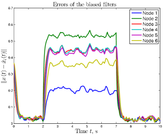
Figure 2: Norms of the errors of the observers (4).

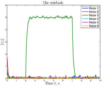
Figure 3: Norms of the residual outputs $\hat{\varepsilon}_{i}(t)$ of the attack detectors (3.2). All residuals except that at the misappropriated node 2, have low amplitude and only respond to disturbances in the system. On the other hand, the residual $\hat{\varepsilon}_{2}(t)$ is able to detect and track the biasing input $f_{2}(t)$.

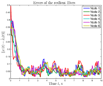
Figure 4: Norms of the errors of the resilient estimates (53), produced using the biased observers (4) augmented with the attack detectors (3.2).

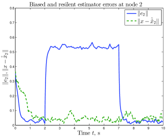
Figure 5: Norms of the errors of the biased and resilient estimates at the misappropriated node 2. The error of the resilient observer incorporating the attack detector is substantially lower than the error of the corresponding observer of the biased network. The estimate (53) at this node appears to be not affected by the attack, it maintains roughly the same level of accuracy during the attack as before and after the attack. However, the error is somewhat greater than the error of the original observer from [27] when it operates normally.

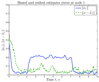
Figure 6: Norms of the errors of the biased and resilient estimates at node 1, which is most distant from the misappropriated node. Even at the most distant node, the error of the resilient observer incorporating the attack detector is almost half of the error of the corresponding observer of the biased network. The error appears to be unaffected by the attack, although it is somewhat greater than the error of the original observer from [27] when it operates normally.

8 Conclusion

The paper is concerned with the problem of distributed attack detection in sensor networks. We consider a group of consensus-based distributed estimators and assume that the estimator dynamics are under attack. Then we propose a distributed attack detector which allows for an uncertainty in the sensors and the plant model, as well as a range of bias attack inputs, and show that the proposed attack detector can detect an biasing attack and identify the misappropriated node. Also, we show that these detectors can be used to compensate the biasing effect of the attack, once it is detected. Although under normal circumstances, the proposed resilient estimates are less accurate than the estimates produced by the original network, they show superior resilience to the attack, in that they asymptotically converge to the state of the plant under a broad range of $L_{2}$ integrable perturbations and biasing attack inputs. The limitation of the proposed scheme lies in the assumption that in principle, admissible attack inputs can be tracked using a low-pass filter and that the tracking error is $L_{2}$ integrable. This restricts the class of attack inputs that can be detected and countered using our approach. Future effort will be directed towards relaxing this assumption.

Another future problem is to consider link failures under denial of service attacks which aim to disrupt the normal flow of information within the network. Sparse networks are more likely to fail under a jamming attack, and for the observer to maintain resilience, additional connectivity within the network may be required. This contrasts with the problem considered in this paper where the attacker relies on dense connectivity to spread the biased $\hat{x}_{i}$ across the network. In this situation, sparse topologies appear to be beneficial for the defender. An interesting problem would be to determine which strategy is more beneficial for the attacker facing a particular network (biasing, jamming or a combination of both), and which network structure provides for the best resilient performance under this strategy. We leave this challenging problem for future research.

Appendix

8.1 Proof of equation (9)

Observe that an input $f_{i}$ of class $\mathscr{F}$ has a Laplace transform of the form $f_{i}(s)=\frac{R_{0}}{s}+\sum_{k}\frac{R_{k}}{(s+p_{k})^{l_{k}}}$ with $\mathrm{Re}(p_{k})<0$, $l_{k}\geq 1$, $\forall k$. By assumption, $(I+\frac{1}{s}G_{i}(s))^{-1}$ has all its poles in the region $\mathrm{Re}(s)<0$, therefore $\forall f_{i}\in\mathscr{F}$,

$$\nu_{i}(s)=-(I+\frac{1}{s}G_{i}(s))^{-1}f_{i}(s)=\frac{\hat{R}_{0}}{s}+\sum_{k}\frac{\hat{R}_{k}}{(s+\hat{p}_{k})^{\hat{l}_{k}}}$$

with $\mathrm{Re}(\hat{p}_{k})<0$, $\hat{l}_{k}\geq 1$, $\forall k$. This time the summation is carried out over the joint set of poles which includes stable poles of both $(I+\frac{1}{s}G_{i}(s))^{-1}$ and $f_{i}(s)$. Hence $\lim_{t\to\infty}\nu_{i}(t)$ exists. Furthermore,

$$\|s\nu_{i}(s)\|\leq\|(I+\frac{1}{s}G_{i}(s))^{-1}\|\cdot\|sf_{i}(s)\|$$

and $\lim_{s\to 0}\|sf_{i}(s)\|=\lim_{t\to\infty}\|f_{i}(t)\|<\infty$. Then according to the final value theorem,

$$\lim_{t\to\infty}\|f_{i}(t)-\hat{f}_{i}(t)\| \leq \lim_{s\to 0}\left(\|(I+\frac{1}{s}G_{i}(s))^{-1}\|\cdot\|sf_{i}(s)\|\right)=0.$$

8.2 Proof of Lemma 1

Let $V=\sum_{i=1}^{N}V_{i}$. Adding the inequalities (24) and selecting $\pi_{i}<\frac{2\alpha_{i}}{q_{i}}$ will result in

$$\dot{V}+\sum_{i=1}^{N}(\delta_{i}^{\prime}Q_{i}\delta_{i}+z_{i}^{\prime}\tilde{Q}_{i}z_{i})$$ (80)

$$\leq-\rho V+\gamma^{2}\sum_{i=1}^{N}(\|\xi\|^{2}+\|\xi_{i}\|^{2}+\|\nu_{i}\|^{2});$$

here $\rho=\min_{i}(2\alpha_{i}-q_{i}\pi_{i})>0$. This implies that when $\xi=0$ and $f_{i}=0$, $\xi_{i}=0$ $\forall i$, then $\dot{V}<-\rho V,$ and since $\mathbf{X}_{i}>0$, we have $z_{i}\to 0$, $\delta_{i}\to 0$ exponentially. That is, condition (i) of Problem 1 is established.

Also, when at least one of the signals $\xi$, $\xi_{i}$ or $f_{i}$ is not equal to zero (the latter is equivalent to $\nu_{i}\not\equiv 0$), then it follows from (80) that with $Q_{i}$, $\bar{Q}_{i}$ defined in (25),

$$\begin{split}\sum_{i=1}^{N}&\int_{0}^{T}(\delta_{i}^{\prime}Q_{i}\delta_{i}+z_{i}^{\prime}\bar{Q}_{i}z_{i})dt\leq\sum_{i=1}^{N}\left[V_{i}(z_{i}(0),\delta_{i}(0))\right.\\ &+\left.\gamma^{2}\int_{0}^{T}(\|\xi\|^{2}+\|\xi_{i}\|^{2}+\|\nu_{i}\|^{2})dt\right].\end{split}$$

Note that $V_{i}(z_{i}(0),\delta_{i}(0))=x_{0}^{\prime}\mathbf{X}_{i}^{11}x_{0}$. Hence (22) also holds with $P=\gamma^{-2}\sum_{i=1}^{N}\mathbf{X}_{i}^{11}$ and $Q_{i}$, $\bar{Q}_{i}$ defined in (25).

8.3 Proof of Lemma 2

With the notation (32) and letting $\mu_{i}=[z_{i}^{\prime}~{}\delta_{i}^{\prime}]^{\prime}$, the system (20) can be represented in the form

$$\dot{\mu}_{i} = (\mathbf{A}_{i}-\mathbf{L}_{i}\mathbf{C}_{i})\mu_{i}+\sum_{j\in\mathbf{V}_{i}}\mathbf{K}_{i}\mathbf{H}(\mu_{j}-\mu_{i})$$ (81)

$$+ \mathbf{B}_{1i}\nu_{i}-(\mathbf{B}_{2}+\mathbf{L}_{i}\mathbf{D}_{i})w_{i}(t),\qquad$$

$$\mu_{i}(0) = \left[\begin{array}[]{c}z_{i}(0)\\ \delta_{i}(0)\end{array}\right],\quad w_{i}\triangleq\left[\begin{array}[]{c}\xi\\ \xi_{i}\end{array}\right].$$ (86)

To establish the vector dissipativity properties of the system (81) we proceed as in [28, 29].

By pre-multiplying and post-multiplying the matrix inequality (52) by $[\mu_{i}^{\prime}~{}\phi_{1}^{\prime}~{}\phi_{2}^{\prime}~{}\mu_{j_{1}}^{\prime}~{}\cdots\mu_{j_{p_{i}}}^{\prime}]$ and its transpose we obtain

$$0> 2\mu_{i}^{\prime}\mathbf{X}_{i}(\mathbf{A}_{i}+\alpha_{i}I-\mathbf{L}_{i}\mathbf{C}_{i})\mu_{i}+2\mu_{i}^{\prime}\mathbf{X}_{i}\mathbf{K}_{i}\mathbf{H}\sum_{j\in\mathbf{V}_{i}}\mu_{j}$$

$$+2\gamma^{2}\mu_{i}^{\prime}\mathbf{C}_{i}^{\prime}\mathbf{E}_{i}^{-1}\mathbf{C}_{i}\mu_{i}-2p_{i}\mu_{i}^{\prime}\mathbf{X}_{i}\mathbf{K}_{i}\mathbf{H}\mu_{i}$$

$$+\mu_{i}^{\prime}\mathbf{Q}_{i}\mu_{i}-\gamma^{2}\mu_{i}^{\prime}\mathbf{C}_{i}^{\prime}\mathbf{E}_{i}^{-1}\mathbf{C}_{i}\mu_{i}-\gamma^{2}\|\phi_{1}-\frac{1}{\gamma^{2}}\mathbf{B}_{1i}^{\prime}\mathbf{X}_{i}\mu_{i}\|^{2}$$

$$+\frac{1}{\gamma^{2}}\mu_{i}^{\prime}\mathbf{X}_{i}\mathbf{B}_{1i}\mathbf{B}_{1i}^{\prime}\mathbf{X}_{i}\mu_{i}-\gamma^{2}\|\phi_{2}-\frac{1}{\gamma^{2}}\left(I-\mathbf{D}_{i}^{\prime}\mathbf{E}_{i}^{-1}\mathbf{D}_{i}\right)\mathbf{B}_{2}^{\prime}\mathbf{X}_{i}\mu_{i}\|^{2}$$

$$+\frac{1}{\gamma^{2}}\mu_{i}^{\prime}\mathbf{X}_{i}\mathbf{B}_{2}\left(I-\mathbf{D}_{i}^{\prime}\mathbf{E}_{i}^{-1}\mathbf{D}_{i}\right)\mathbf{B}_{2}^{\prime}\mathbf{X}_{i}\mu_{i}-\sum_{j\in\mathbf{V}_{i}}\pi_{j}\mu_{j}^{\prime}\mathbf{X}_{j}\mu_{j}.$$

Note that $\left(I-\mathbf{D}_{i}^{\prime}\mathbf{E}_{i}^{-1}\mathbf{D}_{i}\right)$ is a projection matrix and thus $\left(I-\mathbf{D}_{i}^{\prime}\mathbf{E}_{i}^{-1}\mathbf{D}_{i}\right)\left(I-\mathbf{D}_{i}^{\prime}\mathbf{E}_{i}^{-1}\mathbf{D}_{i}\right)=\left(I-\mathbf{D}_{i}^{\prime}\mathbf{E}_{i}^{-1}\mathbf{D}_{i}\right).$ Furthermore, it can be shown by direct calculations that $\frac{1}{\gamma^{2}}\mathbf{B}_{2}\left(I-\mathbf{D}_{i}^{\prime}\mathbf{E}_{i}^{-1}\mathbf{D}_{i}\right)\mathbf{B}_{2}^{\prime}=\frac{1}{\gamma^{2}}(\mathbf{B}_{2}+\mathbf{L}_{i}\mathbf{D}_{i})(\mathbf{B}_{2}+\mathbf{L}_{i}\mathbf{D}_{i})^{\prime}-\gamma^{2}\mathbf{X}_{i}^{-1}\mathbf{C}_{i}^{\prime}\mathbf{E}_{i}^{-1}\mathbf{C}_{i}\mathbf{X}_{i}^{-1}.$ Hence for any vector $[\mu_{i}~{}\mu_{j_{1}}~{}\cdots\mu_{j_{p}}]\neq 0$, letting $\phi_{2}=\frac{1}{\gamma^{2}}\left(I-\mathbf{D}_{i}^{\prime}\mathbf{E}_{i}^{-1}\mathbf{D}_{i}\right)\mathbf{B}_{2}^{\prime}\mathbf{X}_{i}\mu_{i}$ and $\phi_{1}=\frac{1}{\gamma^{2}}\mathbf{B}_{1i}^{\prime}\mathbf{X}_{i}\mu_{i}$ leads to the inequality

$$0> 2\mu_{i}^{\prime}\mathbf{X}_{i}(\mathbf{A}_{i}+\alpha_{i}I-\mathbf{L}_{i}\mathbf{C}_{i})\mu_{i}+\mu_{i}^{\prime}\mathbf{Q}_{i}\mu_{i}-\sum_{j\in\mathbf{V}_{i}}\pi_{j}\mu_{j}^{\prime}\mathbf{X}_{j}\mu_{j}$$

$$+\gamma^{2}\|\nu_{i}-\frac{1}{\gamma^{2}}(\mathbf{B}_{1i})^{\prime}\mathbf{X}_{i}\mu_{i}\|^{2}+2\mu_{i}^{\prime}\mathbf{X}_{i}\mathbf{B}_{1i}\nu_{i}-\gamma^{2}\|\nu_{i}\|^{2}$$

$$+\gamma^{2}\|w_{i}+\frac{1}{\gamma^{2}}(\mathbf{B}_{2}+\mathbf{L}_{i}\mathbf{D}_{i})^{\prime}\mathbf{X}_{i}\mu_{i}\|^{2}-\gamma^{2}\|w_{i}\|^{2}$$

$$-2\mu_{i}^{\prime}\mathbf{X}_{i}(\mathbf{B}_{2}+\mathbf{L}_{i}\mathbf{D}_{i})w_{i}+2\mu_{i}^{\prime}\mathbf{X}_{i}\mathbf{K}_{i}\mathbf{H}\sum_{j\in\mathbf{V}_{i}}(\mu_{j}-\mu_{i}).$$

Then it follows from the above inequality that

$$\dot{V}_{i}\leq-2\alpha_{i}\mu_{i}^{\prime}\mathbf{X}_{i}\mu_{i}-\mu_{i}^{\prime}\mathbf{Q}_{i}\mu_{i}+\gamma^{2}\|\nu_{i}\|^{2}+\gamma^{2}\|w_{i}\|^{2}+\sum_{j\in\mathbf{V}_{i}}\pi_{j}\mu_{j}^{\prime}\mathbf{X}_{j}\mu_{j}.$$

Thus for all $i=1,\cdots,N$ the inequality (24) holds.

References

- [1] T. Başar, and P. Bernhard. optimal control and related minimax design problems: A dynamic game approach. Springer, 2008.
- [2] G. Battistelli and L. Chisci. Kullback-Leibler average, consensus on probability densities, and distributed state estimation with guaranteed stability. Automatica, 50:707–718, 2014.
- [3] D. Bertsekas and J. N. Tsitsiklis. Parallel and distributed computation: Numerical methods. Prentice-Hall, 1989.
- [4] S. Boyd. Distributed optimization and statistical learning via the alternating direction method of multipliers. Foundations and Trends in Machine Learning, 3(1):1–122, 2010.
- [5] M. Deghat, V. Ugrinovskii, I. Shames and C. Langbort. Detection of biasing attacks on distributed estimation networks. In Proc. 55th IEEE CDC, Las Vegas, NV, 2016.
- [6] M. Doostmohammadian and U. A. Khan. On the genericity properties in distributed estimation: Topology design and sensor placement. IEEE Journal of Selected Topics in Signal Processing, 7(2): 195–204, 2013.
- [7] R.M. Ferrari, T. Parisini, M.M. Polycarpou. Distributed fault detection and isolation of large-scale discrete-time nonlinear systems: An adaptive approximation approach. IEEE Trans. Autom. Contr. 57:275–290, 2012.
- [8] X. Ge, Q. L. Han, and X. Jiang. Distributed fault detection for sensor networks with Markovian sensing topology. In Proc. American Control Conference (ACC), pages 3555–3560, 2013.
- [9] W. M. Haddad, V. Chellaboina, and S. G. Nersesov. Vector dissipativity theory and stability of feedback interconnections for large-scale non-linear dynamical systems. Int. J. Contr., 77(10):907–919, 2004.
- [10] X. He, Z. Wang, Y. D. Ji, and D. H. Zhou. Robust fault detection for networked systems with distributed sensors. IEEE Transactions on Aerospace and Electronic Systems, 47(1):166–177, 2011.
- [11] J. P. Hespanha. Linear systems theory. Princeton University Press, 2009.
- [12] I. Hwang, S. Kim, Y. Kim, and C. F. Seah, A survey of fault detection, isolation, and reconfiguration methods. IEEE Transactions on Control Systems Technology, 18(3), 636–653, 2010.
- [13] J. Löfberg. YALMIP: a toolbox for modeling and optimization in MATLAB. In Proc. CACSD Conf., Taipei, Taiwan, pages 284–289, 2004.
- [14] A. Mitra and S. Sundaram. Secure distributed observers for a class of linear time invariant systems in the presence of byzantine adversaries. In Proc. 55th IEEE CDC, 2016.
- [15] A. Mitra and S. Sundaram. Distributed observers for LTI systems. IEEE Trans. Automat. Contr., 2018. DOI 10.1109/TAC.2018.2798998.
- [16] A. Mitra and S. Sundaram. Resilient Distributed State Estimation for LTI Systems. arXiv:1802.09651 (2018).
- [17] R. Olfati-Saber. Distributed Kalman filtering for sensor networks. In Proc. 46th IEEE CDC, pages 5492–5498, 2007.
- [18] S. Park and N. C. Martins. Design of distributed LTI observers for state omniscience. IEEE Trans. Automat. Contr., 62:561–576, 2017.
- [19] F. Pasqualetti, A. Bicchi, and F. Bullo. Consensus computation in unreliable networks: A system theoretic approach. IEEE Trans. Automat. Contr., 57:90-104, 2012.
- [20] F. Pasqualetti, F. Dorfler, and F. Bullo. Attack detection and identification in cyber-physical systems. IEEE Trans. Automat. Contr., 58:2715-2729, 2013.
- [21] F. Pasqualetti, F. Dorfler, and F. Bullo. Control-theoretic methods for cyberphysical security: Geometric principles for optimal cross-layer resilient control systems. IEEE Control Systems, 35:110-127, 2015.
- [22] R. J. Patton and J. Chen. Observer-based fault detection and isolation: Robustness and applications. Contr. Eng. Practice, 5: 671–682, 1997.
- [23] G. S. Seyboth and F. Allgöwer. Output synchronization of linear multi-agent systems under constant disturbances via distributed integral action. In Proc. American Control Conference (ACC), pages 62–67, 2015.
- [24] B. Shen, Z. Wang, and Y. S. Hung. Distributed -consensus filtering in sensor networks with multiple missing measurements: The finite-horizon case. Automatica, 46(10):1682 – 1688, 2010.
- [25] A. Teixeira, I. Shames, H. Sandberg, and K. H. Johansson. Distributed fault detection and isolation resilient to network model uncertainties. IEEE Transactions on Cybernetics, 44(11):2024 – 2037, 2014.
- [26] A. Teixeira, I. Shames, H. Sandberg, and K. H. Johansson. A secure control framework for resource-limited adversaries. Automatica, 51: 135 – 148, 2015.
- [27] V. Ugrinovskii. Distributed robust filtering with consensus of estimates. Automatica, 47(1):1 – 13, 2011.
- [28] V. Ugrinovskii. Gain-scheduled synchronization of parameter varying systems via relative consensus with application to synchronization of uncertain bilinear systems. Automatica, 50(11):2880–2887, 2014. arXiv:1406.5622 [cs.SY].
- [29] V. Ugrinovskii and C. Langbort. Distributed consensus-based estimation of uncertain systems via dissipativity theory. IET Control Theory & App., 5(12):1458–1469, 2011.
- [30] V. Ugrinovskii and C. Langbort. Controller-jammer game models of Denial-of-Service attacks on control systems operating over packet-dropping links, Automatica, 84:128-141, 2017.
- [31] V. Ugrinovskii. Detectability of distributed consensus-based observer networks: An elementary analysis and extensions. In Proc. 2014 Australian Contr. Conf., 2014
- [32] V. Ugrinovskii. Conditions for detectability in distributed consensus-based observer networks. IEEE Tran. Autom. Contr., 58:2659–2664, 2013.
- [33] L. Wang and A. S. Morse. A distributed observer for a time-invariant linear system. In Proc. 2017 ACC, Seattle, 2017.
- [34] J. Wu, L. Li, V. Ugrinovskii and F. Allgöwer. Distributed filter design for cooperative -type estimation. In Proc. IEEE Multi-Conference on Systems and Control, Sydney, Australia, 2015.