Simulation of unsteady blood flows in a patient-specific compliant pulmonary artery with a highly parallel monolithically coupled fluid-structure interaction algorithm

Abstract

Computational fluid dynamics (CFD) is increasingly used to study blood flows in patient-specific arteries for understanding certain cardiovascular diseases. The techniques work quite well for relatively simple problems, but need improvements when the problems become harder in the case when (1) the geometry becomes complex (from a few branches to a full pulmonary artery), (2) the model becomes more complex (from fluid-only calculation to coupled fluid-structure interaction calculation), (3) both the fluid and wall models become highly nonlinear, and (4) the computer on which we run the simulation is a supercomputer with tens of thousands of processor cores. To push the limit of CFD in all four fronts, in this paper, we develop and study a highly parallel algorithm for solving a monolithically coupled fluid-structure system for the modeling of the interaction of the blood flow and the arterial wall. As a case study, we consider a patient-specific, full size pulmonary artery obtained from CT (Computed Tomography) images, with an artificially added layer of wall with a fixed thickness. The fluid is modeled with a system of incompressible Navier-Stokes equations and the wall is modeled by a geometrically nonlinear elasticity equation. As far as we know this is the first time the unsteady blood flow in a full pulmonary artery is simulated without assuming a rigid wall. The proposed numerical algorithm and software scale well beyond 10,000 processor cores on a supercomputer for solving the fluid-structure interaction problem discretized with a stabilized finite element method in space and an implicit scheme in time involving hundreds of millions of unknowns.

1 Introduction

Millions of people die every year from cardiovascular diseases, representing more than $30\%$ of all global deaths [1]. Computational fluid dynamics (CFD) is useful for understanding certain cardiovascular diseases, for example, in [2], it was shown that the wall shear stress obtained through a steady blood flow simulation is highly correlated to the resistive pulmonary arterial impedance. In most numerical simulations, the wall of the artery is assumed to be rigid, but it is widely believed that a simulation with an elastic wall would produce more valuable results than a fluid-only simulation [3], even though, such calculations are computationally very expensive, and often take days or months of computing time on small computers without lots of processor cores. With the recent development of supercomputers, high-resolution fluid-structure interaction (FSI) computation becomes feasible and there have been several successful applications in, for example, respiratory mechanics [4], aeroelasticity [5], and hemodynamics [6, 7, 8]. However, simulating the unsteady blood flow in a deformable pulmonary artery is challenging because the coupled FSI system is highly nonlinear and the geometry of the computational domain is complex. The nonlinearities come from the nonlinear fluid and solid equations, and also from the dependency of the blood velocity and pressure on the domain movement governed by a harmonic extension equation. Moreover, the complexity of the computational domain makes the generation of a matching fluid and solid mesh rather difficult. In this paper, we extend and investigate a monolithically coupled Newton-Krylov-Schwarz (NKS) algorithm for the FSI simulation of the three-dimensional pulmonary vasculature on a supercomputer with more than 10,000 processor cores.

Generally speaking, there are two approaches for coupling a fluid problem with a solid problem, namely, loose coupling (partitioned) and full coupling (monolithic). In the partitioned method, a fluid problem or a solid equation is calculated first, and then its solution is provided as the boundary condition of the other domain. The partitioned algorithm is essentially a Gauss-Seidel iteration, and it has been successfully applied to a few engineering areas, for example, aeroelasticity [5, 9]. But there are two major drawbacks in the partitioned method. First, it is not suitable for parallel computing because the Gauss-Seidel iteration is sequential and has a low concurrency [10]. Second, there is an “added-mass effect”, in other words, significant numerical instabilities are introduced when the densities of the fluid and the solid are close to each other [11]. In this paper, a monolithic approach is employed since it does not suffer from such difficulties and often offers a stable and scalable parallel algorithm. The monolithic approach has been used in several computational hemodynamics applications [3, 6, 7, 8]. In our current work, a nonlinear elasticity equation is used to model the wall of the artery, an incompressible Navier-Stokes system is employed to model the blood flow, and a third equation is used to describe the moving fluid domain. All three partial differential equations are monolithically coupled together based on an Arbitrary Lagrangian Eulerian (ALE) framework [12]. To discretize the coupled FSI system, a $P_{1}$ finite element is utilized for both the solid and domain movement equations and a stabilized $P_{1}-P_{1}$ finite element pair is employed for the incompressible Navier-Stokes equations. The resulting semi-discretized FSI system of equations is further discretized in time using an backward Euler scheme. After the spatial and temporal discretization, a large and highly nonlinear system of algebraic equations is produced and its solution requires an efficient parallel algorithm since we are aiming for a supercomputer with a large number of processor cores, without which the calculation may take days or months of computing time. To tackle the discretized FSI system, we develop an inexact Newton method for solving the nonlinear system, during each Newton iteration a Krylov subspace method together with a Schwarz preconditioner is carefully chosen for the solution of the Jacobian system.

We next briefly review some recent progresses of numerical simulation of blood flows in the pulmonary artery. For the fluid-only calculation, in [13], the blood flow is described by a one-dimensional model discretized with a finite element method, and the corresponding system of nonlinear equations is solved via a quasi Newton method. In [14], a three-dimensional simulation of unsteady blood flows of a patient-specific pulmonary artery is obtained using a stabilized finite element method for the incompressible Navier-Stokes equations, and the sequential simulation takes a couple of days of computing time for a problem with a million elements. In [15], a multiscale model of a one-dimensional pulmonary network is presented and used to analyze the arterial and venous pressure, and the flow. For the FSI simulation, in [16, 17], the CFD-ACE multiphysics package [18] is used for a two-dimensional unsteady blood flow simulation, where a finite volume method is used for the fluid equations and a finite element method is used for the arterial wall. The resulting system of equations is solved with an algebraic multigrid method for the fluid equations and a direct method for the solid equations. A three-dimensional pulmonary arterial bifurcation with simple geometry is simulated by solving a steady state FSI problem in [19], where an in-house FEM code is used to calculate the nonlinear deformation of the thin-walled structure and a commercial CFD solver, ANSYS [20], is used to resolve the fluid equations.

Most of these published works focus on either the fluid only simulation or FSI simulations with simple geometry; i.e., a small number of branches. To best of our knowledge, unsteady 3D FSI simulation with the full patient-specific pulmonary artery is still not available in the existing literature because the required scalable parallel algorithm and software are difficult to develop. Existing commercial software such as ANSYS [20] scales only to a few hundred processor cores, and that’s not enough to carry out these large calculations in a reasonable amount of time. The monolithically coupled NKS was previously applied to a FSI simulation with a small portion of a three-dimensional artery [6, 7, 21, 22], but the approach is not easy to be used for the full artery case since some of the algorithmic parameters are geometry-dependent and problem-dependent; as the complexity of the geometry increases the convergence becomes problematic. With the right choices of parameters, including the subdomain overlap, the fill-in level of incomplete LU factorization, the reordering schemes of the subdomain matrices, the lag of the Jacobian computation and the inexactness of the Newton iterations, we show experimentally that the proposed version of NKS method is scalable with up to 10,240 processor cores for the FSI simulation of a full pulmonary network. We also want to mention that NKS has also been successfully used in different applications in our previous work; unsteady blood flow simulation [23], nonlinear elasticity equations [24], and transient multigroup neutron diffusion equations [10].

The remainder of this paper is organized as follows. In Section 2, we present the physics models used in the FSI coupling and their spatial and temporal discretization. A fully implicit, monolithically coupled parallel Newton-Krylov-Schwarz method is described in Section 3. In Section 4, some numerical experiments and observations are presented, and we focus mainly on the parallel performance of the proposed approach. Lastly, some concluding remarks are given in Section 5.

2 Mathematical models of the fluid and the wall

The pulmonary circulation carries deoxygenated blood from the right ventricle to the lungs. A patient-specific complete pulmonary tree, shown in Fig. 1, is considered in this work.

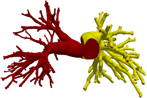
Figure 1: A patient-specific pulmonary artery. The red part is the blood flow domain and the yellow is the arterial wall.

In Fig. 1, the red part is the blood flow domain, and the yellow part is the arterial wall. The cut out is for the visualization, and the entire arterial wall is included in the actual FSI simulation. In this section we describe the models for the blood flow and the arterial wall, as well as the spatial and temporal discretization of the equations.

2.1 Mathematical models for blood flow, arterial wall, and moving fluid domain

We begin by introducing some notations. At time $t\in[0,T]$, let $\Omega_{f}^{t}\in R^{3}$ be the fluid domain, $\Omega_{s}^{t}\in R^{3}$ the arterial wall, $\Gamma^{t}_{f,I}$ the fluid inlet, $\Gamma^{t}_{f,o_{i}},i=1,2,....$ the fluid outlets, $\Gamma^{t}_{s,I}$ the wall inlet, $\Gamma^{t}_{s,o_{i}}$ the wall outlets, $\Gamma^{t}_{s,n}$ the wall outer surface and $\Gamma^{t}_{w}$ the wet interface between the fluid and the arterial wall. Note that $t=0$ corresponds to the initial configuration. The FSI configuration is shown in Fig. 2, where an ALE mapping is defined for tracking the movement of the fluid domain:

$$A_{t}:\mbox{\boldmath$x$}_{f}=A_{t}(\mbox{\boldmath$X$}_{f})\equiv\mbox{\boldmath$X$}_{f}+\mbox{\boldmath$d$}_{m},\mbox{\boldmath$x$}_{f}\in\Omega_{f}^{t},\mbox{\boldmath$X$}_{f}\in\Omega_{f}^{0}.$$

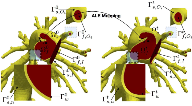
Figure 2: The figure shows the ALE mapping $A_{t}$ from the initial configuration (left) to the configuration at time $t$ (right). In the right figure one can also see the deformation of the arterial wall and the blood flow domain.

We denote by $\mbox{\boldmath$d$}_{m}\in R^{3}$ as the fluid domain displacement at time $t$, and assume it satisfies the following harmonic extension equation

$$\left\{\begin{array}[]{lllll}-\Delta\mbox{\boldmath$d$}_{m}=\bm{0}&\text{~{}in~{}}\Omega_{f}^{0},\\ \mbox{\boldmath$d$}_{m}=\bm{0}&\text{~{}on~{}}\Gamma_{f}^{0}\equiv\Gamma^{0}_{f,I}\cup\Gamma^{0}_{f,O_{i}},i=1,2,...\\ \mbox{\boldmath$d$}_{m}=\mbox{\boldmath$d$}_{s}&\text{~{}on~{}}\Gamma_{w}^{0}.\end{array}\right.$$ (1)

Note that this equation doesn’t have any particular physical meaning, and it is used to describe the motion of the fluid domain. We denote by $\mbox{\boldmath$d$}_{s}\in R^{3}$ as the arterial wall displacement governed by an unsteady, geometrically nonlinear elasticity equation [25] as follows:

$$\left\{\begin{array}[]{llll}\rho_{s}\displaystyle\frac{\partial^{2}\mbox{\boldmath$d$}_{s}}{\partial t^{2}}+\eta_{s}\frac{\partial\mbox{\boldmath$d$}_{s}}{\partial t}-\nabla\cdot\mbox{\boldmath$\Pi$}_{s}=\rho_{s}\mbox{\boldmath$f$}_{s}&\text{~{}in~{}}\Omega_{s}^{0},\\ \mbox{\boldmath$\Pi$}_{s}\mbox{\boldmath$n$}_{s}=\mbox{\boldmath$g$}_{s}&\text{~{}on~{}}\Gamma_{s,n}^{0},\\ \mbox{\boldmath$d$}_{s}=\bm{0}&\text{~{}on~{}}\Gamma_{s,I}^{0}\cup\Gamma_{s,O_{i}}^{0},i=1,2,...\\ \mbox{\boldmath$\sigma$}_{s}{\hat{\mbox{\boldmath$n$}}}_{s}=-\mbox{\boldmath$\sigma$}_{f}\mbox{\boldmath$n$}_{f}&\text{~{}on~{}}\Gamma_{w}^{t}.\end{array}\right.$$ (2)

In (2), $\rho_{s}$ is the wall density, $\mbox{\boldmath$f$}_{s}$ is a volumetric force per unit of mass, $\eta_{s}\partial\mbox{\boldmath$d$}_{s}/\partial t$ is a damping term used to mimic the impact of the surrounding tissues, $\eta_{s}$ is a damping parameter, $\mbox{\boldmath$n$}_{s}$ and ${\hat{\mbox{\boldmath$n$}}}_{s}$ are the unit outward normal vectors (they are related by the Nanson formula [25]) under the initial configuration and the deformed domain, respectively, $\mbox{\boldmath$\sigma$}_{s}$ is the Cauchy stress tensor of the wall, and $\mbox{\boldmath$\sigma$}_{f}$ is the Cauchy stress tensor for the fluid domain to be defined shortly. Here $\mbox{\boldmath$\Pi$}_{s}$ is the nonsymmetric first Piola-Kirchhoff stress tensor for the Saint Venant-Kirchhoff material,

$$\begin{array}[]{llll}\mbox{\boldmath$F$}=(\mbox{\boldmath$I$}+\nabla\mbox{\boldmath$d$}_{s}),\\ \displaystyle\mbox{\boldmath$E$}=\frac{1}{2}({\mbox{\boldmath$F$}}^{T}\mbox{\boldmath$F$}-\mbox{\boldmath$I$}),\\ \mbox{\boldmath$S$}=\lambda_{s}\text{trace}(\mbox{\boldmath$E$})\mbox{\boldmath$I$}+2\mu_{s}\mbox{\boldmath$E$},\\ \mbox{\boldmath$\Pi$}_{s}=\mbox{\boldmath$F$}\mbox{\boldmath$S$},\end{array}$$

where $I$ is a $3\times 3$ identity matrix, $F$ is the deformation gradient tensor, $E$ is the Green-Lagrangian strain tensor, $S$ is the second Piola-Kirchhoff stress tensor, and $\mu_{s}$ and $\lambda_{s}$ are the material Lam$\acute{e}$ constants expressed as functions of Young’s modulus, $E_{s}$, and Poisson’s ratio, $\nu_{s}$, by

$$\mu_{s}=\frac{E_{s}}{2\left(1+\nu_{s}\right)}\text{ and }\lambda_{s}=\frac{E_{s}\nu_{s}}{\left(1+\nu_{s}\right)\left(1-2\nu_{s}\right)}.$$

The nonsymmetric first Piola-Kirchhoff stress tensor $\mbox{\boldmath$\Pi$}_{s}$ and the Cauchy stress tensor $\mbox{\boldmath$\sigma$}_{s}$ are related by the formula:

$$\mbox{\boldmath$\sigma$}_{s}=\frac{\mbox{\boldmath$\Pi$}_{s}\mbox{\boldmath$F$}^{T}}{det(\mbox{\boldmath$F$})}.$$

Here $det(\mbox{\boldmath$F$})$ is the determinant of the tensor $F$. For the blood flows, let ${\mbox{\boldmath$u$}}_{f}$ and $p_{f}$ denote the velocity and the pressure, respectively, and the incompressible Navier-Stokes equations on the moving domain are presented as follows

$$\centering\left\{\begin{array}[]{llllll}\displaystyle\left.\rho_{f}\frac{\partial{\mbox{\boldmath$u$}}_{f}}{\partial t}\right|_{\mbox{\boldmath$X$}_{f}}+\rho_{f}\left[\left({\mbox{\boldmath$u$}}_{f}-\frac{\partial\mbox{\boldmath$d$}_{m}}{\partial t}\right)\cdot\nabla\right]{\mbox{\boldmath$u$}}_{f}\displaystyle-\nabla\cdot\mbox{\boldmath$\sigma$}_{f}=\rho_{f}\mbox{\boldmath$f$}_{f}&\text{~{}in~{}}\Omega^{t}_{f},\\ \nabla\cdot{\mbox{\boldmath$u$}}_{f}=0&\text{~{}in~{}}\Omega^{t}_{f},\\ \displaystyle{\mbox{\boldmath$u$}}_{f}=\mbox{\boldmath$v$}_{f}^{d}&\text{~{}on~{}}\Gamma^{t}_{f,I},\\ \displaystyle\mbox{\boldmath$\sigma$}_{f}\mbox{\boldmath$n$}_{f}=\mbox{\boldmath$g$}_{f}&\text{~{}on~{}}\Gamma^{t}_{f,O_{i}},\\ \displaystyle{\mbox{\boldmath$u$}}_{f}=\frac{\partial\mbox{\boldmath$d$}_{s}(A_{t}^{-1})}{\partial t}&\text{~{}on~{}}\Gamma^{t}_{w},\end{array}\right.\@add@centering$$ (3)

where $\rho_{f}$ is the fluid density, $|_{\mbox{\boldmath$X$}_{f}}$ indicates that the time derivative is taken under the ALE configuration, $\partial\mbox{\boldmath$d$}_{m}/\partial t$ is the velocity of the mesh movement, $\mbox{\boldmath$f$}_{f}$ is a volumetric force per unit of mass, $\mbox{\boldmath$g$}_{f}$ is a traction applied to the outlets, $\mbox{\boldmath$v$}_{f}^{d}$ is a velocity profile prescribed at the inlet, $A_{t}^{-1}$ is a pull-back operator that maps the current coordinates to the original configuration, $\mbox{\boldmath$n$}_{f}$ is the unit outward normal vector for the fluid domain and $\mbox{\boldmath$\sigma$}_{f}$ is the Cauchy stress tensor for the fluid defined as

$$\mbox{\boldmath$\sigma$}_{f}=-p_{f}\mbox{\boldmath$I$}+2\nu_{f}\mbox{\boldmath$\varepsilon$}_{f},~{}\mbox{\boldmath$\varepsilon$}_{f}=\frac{1}{2}\left(\nabla{\mbox{\boldmath$u$}}_{f}+\nabla{\mbox{\boldmath$u$}}_{f}^{T}\right),$$

where $\mbox{\boldmath$\varepsilon$}_{f}$ is the strain rate tensor and $\nu_{f}$ is the viscosity coefficient. On the wet interface, three coupling conditions are imposed to couple the solid and fluid equations. The first condition is the continuity of the velocity: ${\mbox{\boldmath$u$}}_{f}=\partial\mbox{\boldmath$d$}_{s}/\partial t$. The second condition is the continuity of the displacement: $\mbox{\boldmath$d$}_{m}=\mbox{\boldmath$d$}_{s}$. Lastly, the traction forces from the fluid and the solid are the same: $\mbox{\boldmath$\sigma$}_{s}{\hat{\mbox{\boldmath$n$}}}_{s}=-\mbox{\boldmath$\sigma$}_{f}\mbox{\boldmath$n$}_{f}$. These conditions are included in (1), (2) and (3), through which the coupled FSI system is formed.

2.2 Seamless coupling discretization

To discretize (1), (2) and (3), we consider a $P_{1}-P_{1}$ stabilized finite element pair [23, 26, 27] for the incompressible Navier-Stokes equations and a $P_{1}$ finite element method for both the solid equation and the fluid domain moving equation. Interested readers are referred to [21, 22] for more details.

There are two approaches to implement the continuity conditions (the velocity continuity and the displacement continuity) on the wet interface for the displacement and the velocity, that is, they can be formed either weakly or strongly. Let ${\mbox{\boldmath$u$}}_{f}^{h},{\mbox{\boldmath$u$}}_{s}^{h},\mbox{\boldmath$d$}_{m}^{h}$ and $\mbox{\boldmath$d$}_{s}^{h}$ be their counterparts in the finite element spaces. The constraints can be enforced weakly through the following weak forms:

$$\int_{\Gamma_{w}^{h}}({\mbox{\boldmath$u$}}_{f}^{h}-{\mbox{\boldmath$u$}}_{s}^{h})\mbox{\boldmath$v$}\,\mathrm{d}s=0,~{}\forall\mbox{\boldmath$v$}\in\mbox{\boldmath$V$}^{h}$$ (4)

and

$$\int_{\Gamma_{w}^{h}}(\mbox{\boldmath$d$}_{m}^{h}-\mbox{\boldmath$d$}_{s}^{h})\mbox{\boldmath$v$}\,\mathrm{d}s=0,~{}\forall\mbox{\boldmath$v$}\in\mbox{\boldmath$V$}^{h}.$$ (5)

Here $\mbox{\boldmath$V$}^{h}$ is a $P_{1}$ finite element function space defined on the wet interface. In the strong form of the interface condition, the constraints are enforced at every mesh points, that is, $\mbox{\boldmath$d$}_{m}^{h}|_{\Gamma_{w}^{h}}=\mbox{\boldmath$d$}_{s}^{h}|_{\Gamma_{w}^{h}}$ and ${\mbox{\boldmath$u$}}_{f}^{h}|_{\Gamma_{w}^{h}}={\mbox{\boldmath$u$}}_{s}^{h}|_{\Gamma_{w}^{h}}$. Here we think of ${\mbox{\boldmath$u$}}_{f}^{h},{\mbox{\boldmath$u$}}_{s}^{h},\mbox{\boldmath$d$}_{m}^{h}$ and $\mbox{\boldmath$d$}_{s}^{h}$ as nodal values of their corresponding finite element functions without introducing any confusion. More precisely, let $\mbox{\boldmath$d$}^{h}_{\Gamma,m},\mbox{\boldmath$d$}^{h}_{\Gamma,s}$ be the unknowns of the fluid and solid displacements on the wet interface, respectively, and $\mbox{\boldmath$d$}^{h}_{I,m}$, $\mbox{\boldmath$d$}^{h}_{I,s}$ correspond to the unknowns defined in the interior of the domain. To show the matrix structure of the coupling condition on the interface, we take $\mbox{\boldmath$d$}^{h}_{\Gamma_{w},m}=\mbox{\boldmath$d$}^{h}_{\Gamma_{w},s}$ as an example, and the structure of the coupled FSI matrix for the mesh movement and the solid deformation looks like

$$\left[\begin{array}[]{llllll}J^{m}_{I,I}&J^{m}_{I,\Gamma_{w}}\\ 0&I&-I&\\ 0&B&0&\\ 0&0&J^{s}_{I,\Gamma_{w}}&J^{s}_{I,I}\\ \end{array}\right]\left[\begin{array}[]{llllll}\mbox{\boldmath$d$}^{h}_{I,m}\\ \mbox{\boldmath$d$}^{h}_{\Gamma_{w},m}\\ \mbox{\boldmath$d$}^{h}_{\Gamma_{w},s}\\ \mbox{\boldmath$d$}^{h}_{I,s}\\ \end{array}\right]=\left[\begin{array}[]{llllll}0\\ 0\\ 0\\ \mbox{\boldmath$f$}_{s}\\ \end{array}\right].$$ (6)

(6) is reduced to (7) if we replace the wall displacement unknowns $\mbox{\boldmath$d$}_{\Gamma_{w},s}^{h}$ by the fluid displacement unknowns $\mbox{\boldmath$d$}_{\Gamma_{w},m}^{h}$ as follows:

$$\left[\begin{array}[]{llllll}J^{m}_{I,I}&J^{m}_{I,\Gamma_{w}}\\ 0&B&0&\\ 0&J^{s}_{I,\Gamma_{w}}&J^{s}_{I,I}\\ \end{array}\right]\left[\begin{array}[]{llllll}\mbox{\boldmath$d$}^{h}_{I,m}\\ \mbox{\boldmath$d$}^{h}_{\Gamma_{w},m}\\ \mbox{\boldmath$d$}^{h}_{I,s}\\ \end{array}\right]=\left[\begin{array}[]{llllll}0\\ 0\\ \mbox{\boldmath$f$}_{s}\\ \end{array}\right].$$ (7)

A similar procedure can be applied to the continuity condition on the velocity as well. This implementation of the continuity conditions makes the postprocessing more convenient because there are no duplicate unknowns on the interface mesh. For the detailed structure of the coupled FSI system, we refer to our previous work [28].

After the discretization in space, the corresponding semi-discretized system is a time-dependent nonlinear system

$$\frac{\partial y(t)}{\partial t}+N(y(t))=F,$$ (8)

where $F$ is the right-hand side and $N(\cdot)$ is a nonlinear function, $y(\cdot)$ is the time-dependent vector of nodal values of the fluid velocity and pressure, the solid velocity and displacement, and the displacement of the moving fluid domain. Using an implicit first-order backward Euler scheme, (8) is further discretized in time as:

$$M_{n}y_{n}+\delta tN(y_{n})=\delta tF+M_{n}y_{n-1},$$ (9)

where $\delta t$ is the time step size, $y_{n}$ is the approximation of $y$ at the $n$th time step, $M_{n}$ is the mass matrix dependent of $y_{n}$ since the computational fluid domain is moving. The ALE velocity $\partial\mbox{\boldmath$d$}_{m}/\partial t$ is approximated by the first-order backward Euler scheme in (9) as well. For convenience, we rewrite (9) at the $n$th time step as a nonlinear algebraic system:

$$\,\mathcal{F}(y)=0,$$ (10)

where $\,\mathcal{F}(\cdot)$ is the combination of four terms in (9), and $y$ (we drop the subscript $n$ here for simplicity) is the vector of nodal values at the $n$th time step.

Because we want a high resolution simulation of the FSI system, (10) is usually very large, and is quite difficult to solve since all the high nonlinearities are coupled in this single system. In the next section, we discuss a highly parallel, domain decomposition based solver for (10).

3 Monolithic coupling parallel algorithm

The parallel algorithm consists of a Newton method [29] for the coupled nonlinear system, a Krylov subspace method [30] for the Jocabian system and an overlapping domain decomposition preconditioner [31] for the acceleration of the linear solver. With a given initial guess, $y^{(0)}$, inexact Newton obtains a new approximation as follows:

$$y^{(n+1)}=y^{(n)}+\alpha^{(n)}\delta y^{(n)},$$ (11)

where $y^{(n)}$ is the approximate solution at the $n$th Newton step, $\alpha^{(n)}$ is a Newton step size computed using a line search scheme such as backtracking [32], and $\delta y^{(n)}$ is the Newton direction obtained by solving the Jacobian system:

$$\,\mathcal{J}(y^{(\tilde{n})})\delta y^{(n)}=-\,\mathcal{F}(y^{(n)}).$$ (12)

Here $\,\mathcal{J}(y^{(\tilde{n})})$ is the Jacobian matrix evaluated at $y^{(\tilde{n})}$, and $\,\mathcal{F}(y^{(n)})$ is the nonlinear function residual evaluated at $y^{(n)}$. $\tilde{n}$ is smaller than or equal to $n$. The Jacobian matrix from a previous step is reused if $\tilde{n}$ is strictly smaller than $n$.

The convergence of (11) depends critically on how the Jacobian matrix $\,\mathcal{J}$ is constructed and how the Jacobian system (12) is solved. The construction and the solve of the Jacobian are both expensive and therefore carefully designed algorithms are extremely important. To have good nonlinear convergence, the Jacobian matrix $\,\mathcal{F}$ is analytically derived and hand-coded in the C++ code. It is a challenging task to form all derivatives exactly instead of using a finite difference method, but it worth doing so because Newton equipped with an exact Jacobian often has a more robust convergence. To save the compute time, the Jacobian from the previous Newton step may be reused as the evaluation of the Jacobian matrix is expensive. As stated earlier, the system (10) is highly nonlinear, and so the resulting Jacobian system is ill-conditioned. To overcome this difficulty, we propose a Krylov method, GMRES [30] together with a preconditioner based on an overlapping domain decomposition method. The Krylov subspace method is generally understood in the existing literatures, but for it to work well for a specific application, a preconditioner has to be constructed carefully, especially these problem dependent parameters need to be considered. More precisely, instead of (12), the following preconditioned linear system is solved

$$B^{-1}\,\mathcal{J}\delta y=-B^{-1}\,\mathcal{F}.$$ (13)

For simplicity, the arguments of $\,\mathcal{J}(\cdot)$ and $\,\mathcal{F}(\cdot)$ are dropped here. $B^{-1}$ is a parallel preconditioner to be constructed based on an overlapping domain decomposition method below. Note that the same preconditioner can be applied from the right side as well.

The basic idea of domain decomposition methods [31, 33] is to divide the mesh $\Omega_{h}=\Omega_{h,s}\cup\Omega_{h,f}$ into $np$ submeshes $\Omega_{h,i},i=0,1,2...$, and each submesh $\Omega_{h,i}$ is assigned to a processor core and all subproblems are solved simultaneously in parallel. For the overlapping version of domain decomposition methods, the submeshes are extended to overlap with their neighboring submeshes by $\delta$ layers of mesh points. The overlapping submeshes are denoted as $\Omega_{h,i}^{\delta}$. To partition the mesh $\Omega_{h}$ across different processor cores, we employ a hierarchical partitioning method because mesh partitioning software such as ParMETIS/ METIS [34] doesn’t work well for the full pulmonary tree due to the complexity of geometry. The idea of a hierarchical partition is quite simple but very effective. The mesh $\Omega_{h}$ is first partitioned into $np_{1}$ submeshes ($np_{1}$ is the number of compute nodes), then each submesh is further partitioned into $np_{2}$ smaller submeshes ($np_{2}$ is the number of processor cores per compute node), and finally we have $np=np_{1}\times np_{2}$ submeshes in total. The advantage of the hierarchical partitioning method is to take the architecture of modern computers into consideration, and the communication among different compute nodes are minimized. More details of the hierarchical partitioning method are provided in [6, 7, 24].

To describe the preconditioning technique, we denote the vector and submatrix associated with submesh $\Omega_{h,i},$ as $y_{h,i}$ and $\,\mathcal{J}_{h,i}$, and that for the overlapping submesh as $\Omega_{h,i}^{\delta},$ as $y_{h,i}^{\delta}$ and $\,\mathcal{J}_{h,i}^{\delta}$. Let us define a restriction operator $R_{i}^{\delta}$ as

$$y_{h,i}^{\delta}=R_{i}^{\delta}y=(\mbox{\boldmath$I$}~{}0)(y^{\delta}_{h,i}~{}y/y^{\delta}_{h,i})^{T},$$ (14)

where $I$ is an identity matrix whose size is the same as $y_{h,i}^{\delta}$. The restriction operator $R_{i}^{\delta}$ is used to extract a subverter $y_{h,i}^{\delta}$ from the global vector $y$ by selecting the corresponding components. Using $R_{i}^{\delta}$, the overlapping submesh matrix $\,\mathcal{J}_{h,i}^{\delta}$ is written as

$$\,\mathcal{J}_{h,i}^{\delta}=(R_{i}^{\delta})^{T}\,\mathcal{J}R_{i}^{\delta}.$$ (15)

With these ingredients, a restricted Schwarz preconditioner (overlapping domain decomposition method) reads as

$$B^{-1}=\sum_{i=0}^{np-1}(R_{i}^{0})^{T}(\,\mathcal{J}_{h,i}^{\delta})^{-1}(R_{i}^{\delta})^{T},$$ (16)

where $R_{i}^{0}$ is a restriction operator without any overlap, and $(\,\mathcal{J}_{h,i}^{\delta})^{-1}$ represents a subdomain solver that is an incomplete LU factorization in this work.

4 Numerical experiments and observations

In this section, we discuss some results obtained by applying the algorithms developed in the previous sections to the full pulmonary artery. The geometry of the interior of the artery is obtained from the segmentation of a contrast-enhanced CT image of a healthy 19 year-old subject, and the arterial wall is added to the resulting artery manually. The wall thickness is assumed to be $1~{}mm$ everywhere. Note that because of the lack of imaging data for the arterial wall, the artificially added wall may not be physiologically correct, however, the algorithmic framework introduced in this study can be easily applied when the correct wall geometry becomes available.

The main emphasis of the section is the parallel performance of the algorithm which is one of the key factors for obtaining high resolution simulations of patient-specific pulmonary arteries in a reasonably amount of time. For convenience, we introduce some notations and default parameters used in the following study. “NI” is used to represent the number of Newton iterations per time step, “LI” denotes the averaged number of GMRES(fGMRES) iterations pert Newton step, “T” is the total compute time in second for all 10 time steps, “MEM” in megabytes (MB) is the estimated memory usage per processor core, and “efficiency” is the parallel efficiency of the proposed algorithm. ILU(1) is adopted as the subdomain solver, the subdomain overlapping size is 1, and the relative tolerances for Newton and GMRES are $10^{-6}$ and $10^{-3}$ respectively. These parameters are used through the whole performance study, unless otherwise specified. The proposed algorithm is implemented based on PETSc [35].

4.1 Simulation results and discussions

In this section, we report some simulation results obtained by applying the proposed algorithms to the pulmonary artery shown in Fig 1. A velocity profile derived from a given inflow rate shown in Fig 3, is applied to the inlet, while the flows at all outlets are supposed to be traction-free. The fluid is characterized with viscosity $\mu_{f}=0.03~{}g/(cm~{}s)$ and density $\rho_{f}=1~{}g/cm^{3}$. The material parameters of the arterial wall are Young’s modulus $E_{s}=4\times 10^{6}~{}g/(cm~{}s^{2})$, Poisson’s ratio $\mu_{s}=0.42$, and density $\rho_{s}=1.2~{}g/cm^{3}$. The simulation is carried out with the time step size $\delta t=10^{-3}$ for three cardiac cycles, $[0,1.8]$ seconds, and the solution is shown in Fig 4, 5, 6 and 7.

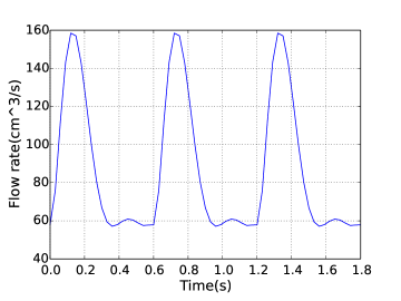
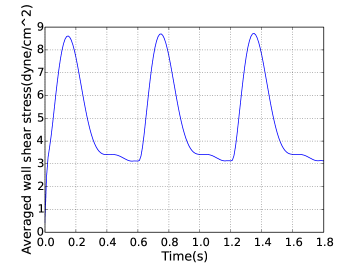
Figure 3: Left: inflow rate for three cardiac cycles, $[0,1.8]$, with 0.6 second per cycle. Right: spatially averaged wall sheer stress.

The wall sheer stress (WSS) is an important metric, and it is calculated by the following formula

$$WSS=\mbox{\boldmath$\sigma$}_{f}\mbox{\boldmath$n$}_{f}-(\mbox{\boldmath$\sigma$}_{f}\mbox{\boldmath$n$}_{f}\cdot\mbox{\boldmath$n$}_{f})\mbox{\boldmath$n$}_{f},$$

and the spatially averaged WSS (SAWSS) is obtained by integrating the WSS on the entire inner surface of the artery and then normalized over the area, that is,

$$SAWSS=\frac{1}{A}\int_{\partial\Omega_{f}}WSSdA,$$

where $A$ is the total area of the inner surface of the pulmonary artery. In Fig. 3, we observe that SAWSS is highly correlated with the input flow rate; SAWSS increases when the input flow rate increases with time, and it decreases when the input flow rate decreases.

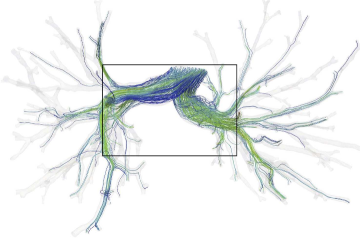
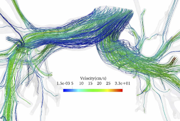
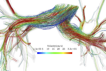
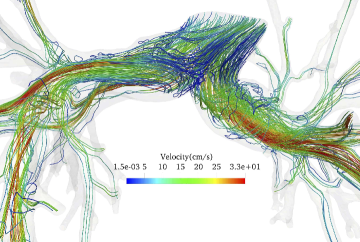
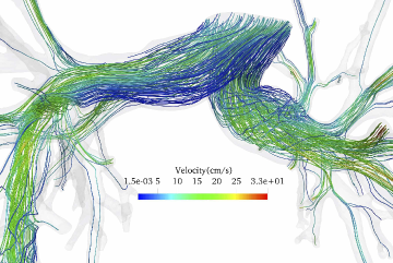
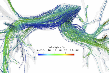
Figure 4: Streamlines of the flow field at $1.2s$ (top right), $1.35s$ (middle left), $1.5s$ (middle right), $1.65s$ (bottom left) and $1.8s$ (bottom right). Top left: the entire blood flow domain; all others: zoom-in pictures for streamlines

In Fig. 4, we see that the velocity is maximized at $1.35s$ when the right ventricle contracts and the inflow rate reaches the maximum, and the flow pattern becomes more complicated at the end of systole, $1.5s$. The flow is periodic in time, and it is restored to a similar pattern at $1.8s$ that is the start of the next cycle.

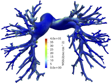
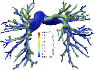
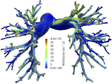
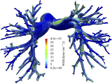
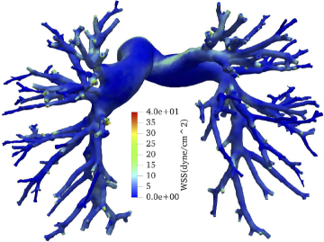
Figure 5: Wall shear stress at $1.2s$ (top left), $1.35s$ (top right), $1.4s$ (middle left), $1.5s$ (middle right), $1.65s$ (bottom left) and $1.8s$ (bottom right).

In Fig 5, at $1.35s$ and $1.4s$, the inner artery wall has the largest wall shear stress in magnitude, and it is correlated to the inflow pattern.

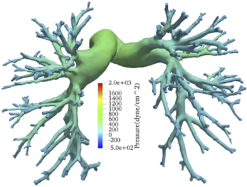
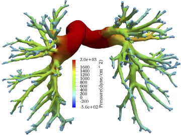
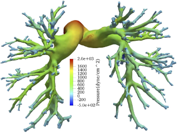
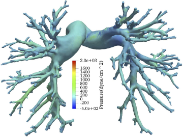
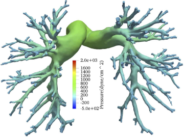
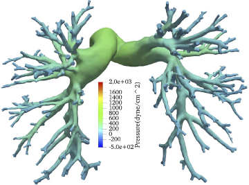
Figure 6: Blood flow pressure at $1.2s$ (top left), $1.35s$ (top right), $1.4s$ (middle left), $1.5s$ (middle right), $1.65s$ (bottom left) and $1.8s$ (bottom right).

In Fig. 6, similarly, the pressure is also highly correlated to the inflow rate, that is, the pressure is high at systole and low at diastole.

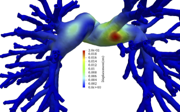
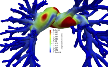
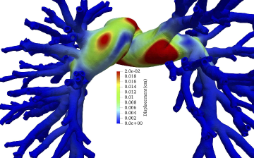
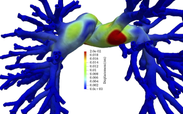
Figure 7: The displacement of the arterial wall at $1.2s$ (top right), $1.35s$ (middle left), $1.4s$ (middle right), $1.5s$ (bottom left) and $1.8s$ (bottom right). For visualization, the displacement is amplified by a factor of 20. The top left picture represents the undeformed domain.

From Fig. 7, it is easily observed that the largest displacements are at $1.35s$ and $1.4s$, and the proximal blood vessels have larger displacements while the ones at the distal do not deform much. In order to further understand how blood flows are different at the proximal and distal vessels, we probe the blood velocity and the pressure at different locations, and the results are shown in Fig. 8, which shows clearly that the pressure decreases from the proximal to the distal, and it is correlated to the inflow wave. The third cycle of pressure wave has the same pattern as the second cycle, which indicates the simulation has reached a quasi steady state. We also have a similar observation for the velocity, except that the velocity magnitude at $L4$ is larger than all other three locations.

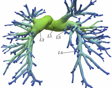
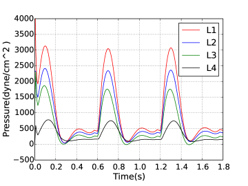
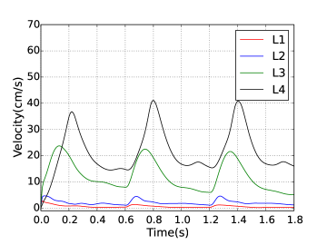
Figure 8: Pressure (left) and velocity (right) at different locations marked in the top picture.

4.2 Linear solver impact on the outer Newton iteration

The accuracy of the linear Jacobian solver has a major impact on the convergence of the outer Newton iterations. More Newton iterations are usually required if the Jacobian system is not solved accurate enough, on the other hand the linear problems should not be over-solved because beyond certain point it does not help the nonlinear solver any more and simply wastes computing time. The accuracy of the linear solver is controlled using a relative tolerance, $\text{L}_{rel}$, where a smaller value indicates a more accurate Newton direction. We next carry out a test to investigate the impact of the linear solver. The mesh used in this test has 2,014,726 vertices and 9,464,723 elements, the problem has 12,793,688 unknowns, and the simulation is carried out for 10 time steps. The overlapping domain decomposition method with ILU(1) as the subdomain solver and $\delta=1$ is used as the preconditioner to accelerate the convergence of the Krylov subspace method GMRES. The algorithm performance using 128 to 1,240 processor cores is summarized in Table 1.

Table 1: Impact of different tolerances of linear solver. A nonlinear system of equations with 12,793,688 unknowns is solved by inexact Newton-Krylov method together with a one-level Schwarz preconditioner. “$\ast$” indicates no convergence

$np$	$\text{L}_{rel}$	NI	LI	T (second)	MEM (MB)	EFF
128	$10^{-1}$	6.8	$13.2$	1255.9	600.4	100%
128	$10^{-2}$	4	19.2	771.8	608.3	100%
128	$10^{-3}$	3.5	23.6	690.3	616.3	100%
128	$10^{-4}$	3	30.4	630.8	616.3	100%
128	$10^{-5}$	2.9	39	632	624.2	100%
256	$10^{-1}$	7.2	$13.9$	719.8	299.6	87%
256	$10^{-2}$	4.8	19.5	509.8	303.6	76%
256	$10^{-3}$	3.9	23.7	420.5	307.6	82%
256	$10^{-4}$	3.4	30.8	384.9	311.6	82%
256	$10^{-5}$	3	40	366.4	311.6	86%
512	$10^{-1}$	$\ast$	$\ast$	$\ast$	$\ast$	$\ast$
512	$10^{-2}$	4.8	20.4	312.3	181	62%
512	$10^{-3}$	3.9	24.9	261.1	183	66%
512	$10^{-4}$	3.2	32.9	224.9	185.1	70%
512	$10^{-5}$	3	41.6	221.2	187.2	71%
1,024	$10^{-1}$	7.2	15.1	244.3	82.7	64%
1,024	$10^{-2}$	4.5	20.3	155.4	83.7	62%
1,024	$10^{-3}$	3.9	25.3	138.6	84.7	62%
1,024	$10^{-4}$	3	33.3	112	85.7	70%
1,024	$10^{-5}$	2.9	42.1	113.2	86.7	70%

It is easily observed from Table 1 that the number of Newton iterations is decreased quickly at the beginning and then slowly when we increase the accuracy of the linear solver by reducing the relative tolerance. For the 128-core case, the averaged number of Newton iterations is decreased from $6.8$ to $4$ when $\text{L}_{rel}$ is reduced from $10^{-1}$ to $10^{-2}$, and when we continue to decrease $\text{L}_{rel}$ by another order of magnitude from $10^{-2}$ to $10^{-3}$, the number of Newton iterations is decreased by only $0.5$. The number of linear iterations per Newton using a loose tolerance is smaller than that using a tight tolerance since more effort is needed for achieving a more accurate Newton direction. Sometimes, if the tolerance is too loose, the overall algorithm may not converge at all because a minimum accuracy is required for Newton to converge. For instance, Newton does not work for the 512-core case when the tolerance is chosen as $\text{L}_{rel}=10^{-1}$. We keep decreasing the tolerance from $10^{-3}$ to $10^{-4}$, and the number of Newton iterations is first reduced by half or one iteration, and it does not change much with a decrease in the tolerance from $10^{-4}$ to $10^{-5}$. The compute time is reduced significantly at the very beginning because the number of Newton iterations is decreased a lot due to a tighter tolerance, and it is decreased slowly thereafter. For example, in the 128-core case, the compute time is $1255.9$ seconds when $\text{L}_{rel}=10^{-1}$, while it is reduced to $771.8$ seconds by almost half with $\text{L}_{rel}=10^{-2}$. The compute time does not reduce much and sometimes slightly increases when the accuracy of the linear solver reaches a certain level. Let us look at the 128-core case again: the compute time is $630.8$ with $\text{L}_{rel}=10^{-4}$, and it is increased by a few seconds to $632$ when we use $\text{L}_{rel}=10^{-4}$. A tighter linear solver helps maintain a great scalability. The parallel efficiency is kept at about $70\%$ when the relative tolerance is chosen as $10^{-4}$ or $10^{-3}$. In all, the difference of compute time using the tolerance of $10^{-3}$ to $10^{-5}$ is small, and hence an arbitrary relative tolerance ranging from $10^{-3}$ to $10^{-5}$ should work well for the problems at hand. The scalability is good for all cases as long as the tolerance is not too loose.

4.3 Subdomain solver: incomplete LU factorization

Incomplete LU (ILU) factorization is a popular subdomain solver for overlapping domain decomposition methods. Like all other solvers, there are a few parameters, in ILU, that affect the overall convergence of the linear solver. Among these parameters, the most important one is the fill-in level that represents how much extra allocation is allowed to store new values introduced by the factorization. Level 0, denoted as ILU(0), indicates that all new extra values are discarded, and the factorized matrix has the same sparsity as the original submatrix. ILU($l$) represents that $l$ layers of extra entries are kept. Larger $l$ usually leads to a better and more robust converge but meanwhile it may slow down the entire solver because more operations and more memory are needed. An optimal fill-in level is also problem-dependent. We perform a test for different fill-in levels, and the results are summarized in Table 2. The same configuration as in the previous test is used.

Table 2: Different fill-in levels for ILU. A nonlinear system of equations with 12,793,688 unknowns is calculated by an one-level Schwarz preconditioner with ILU($l$) as the subdomain solver.

$np$	subsolver	NI	LI	T	MEM	EFF
128	ILU(0)	4.1	72.7	1015.1	552	100%
128	ILU(1)	3.5	23.6	689.4	616.3	100%
128	ILU(2)	3.6	17.3	797.9	800.3	100%
256	ILU(0)	3.9	69.2	507.7	274.7	100%
256	ILU(1)	3.9	23.7	426.6	307.6	81%
256	ILU(2)	3.9	18.2	466.6	397	86%
512	ILU(0)	3.9	68.9	302.3	157.9	84%
512	ILU(1)	3.9	24.9	265.6	183	65%
512	ILU(2)	3.9	18.5	289	242	69%
1,024	ILU(0)	$\ast$	$\ast$	$\ast$	$\ast$	$\ast$
1,024	ILU(1)	3.9	25.3	138	84.7	62%
1,024	ILU(2)	3.9	20.4	152.9	109.2	65%

For the128-core case, when the fill-in level is increased from $0$ to $1$ the number of GRMES iterations is reduced to one-third, which results in the reduction of the compute time by half. When we continue increasing the fill-in level from $1$ to $2$, the number of GMRES iterations is decreased by only $5$, and the compute time is increased due to the increased cost of LU factorization per iteration. For all cases, the number of Newton iterations is kept close to a constant, $4$, because the relative tolerance of GRMES is fixed as $10^{-3}$ regardless of the ILU fill-in level. ILU($0$) sometimes is unstable. For example, Newton does not converge for the case of 1,024 processor cores when ILU(0) is used, while it performs well using ILU(1) and ILU(2). The memory usage is increased slightly when ILU(1) is used instead of ILU(0), while it is increased a lot with the increase of fill-in level from $1$ to $2$. In the128-core case, the memory usage is increased by $70$ MB when we increase the fill-in level from $0$ to $1$, while it is increased by almost $200$ MB with the increase of fill-in level from $1$ to $2$. ILU(1) is the best subdomain solver in this test when we take both the compute time and the memory usage into consideration. For all cases, the overall algorithm scales well when the number of processor cores is increased from $128$ to $1,024$.

4.4 Jacobian reevaluation

By default, the Jacobian matrix is updated at every Newton iteration. Since the evaluation of the Jacobian matrix is expensive, sometimes the overall efficiency of the algorithm is improved by reusing the Jacobian matrix for several Newton iterations. In the rest of this subsection, we denote by ”$lag$” as the number of times that the Jacobian matrix is reused. In this test, we use the same configuration as before to illustrate the behavior of the algorithm when using different lags. The results are shown in Table 3, which shows clearly that

Table 3: Impact of Newton lags on the compute time. A nonlinear system of equations with 12,793,688 unknowns is solved using inexat Newton and each Jacobian matrix is used for $lag$ iterations.

$np$	$lag$	NI	LI	T	MEM	EFF
128	1	3.5	23.6	689.5	616.3	100%
128	2	3.9	22.6	492.5	616.3	100%
128	3	4.1	21.4	485.2	616.3	100%
128	4	4.1	21.1	351.1	616.3	100%
256	1	3.9	23.7	427.8	307.6	81%
256	2	4.3	23.3	304.2	307.6	81%
256	3	4.6	22.4	284.1	307.6	85%
256	4	4.8	21.6	250.3	307.6	70%
512	1	3.9	24.9	261.2	183	66%
512	2	4.1	24.6	169.3	183	73%
512	3	4.8	23.5	171.5	183	71%
512	4	4.9	22.6	160.5	183	55%
1024	1	3.9	25.3	138.7	84.7	62%
1024	2	4.0	25	86.5	84.7	71%
1024	3	4.4	23.8	88.2	84.7	69%
1024	4	4.4	23.1	70.8	84.7	62%

the compute time is significantly reduced when we reuse the Jacobian matrix for two Newton steps instead of one, and then it is improved very little when we further increase $lag$ for all processor counts except the case when the number of cores is 128, where the compute time is reduced by $100$ seconds when $lag$ is increased from $3$ to $4$. The Jacobian lag does not affect the memory usage for all cases because a sparse matrix is always stored regardless of its value updates. The overall algorithm behaves similarly when $lag=2,3$ and $4$, while the performance with $lag=1$ is much worse. The number of Newton iterations increases when we lag the Jacobian matrix evaluation, but the increase is not significant so that we have the benefit of Jacobian lagging. In the 1,024-core case, the compute time is decreased by $50\%$ when we lag the Jacobian evaluation from every Newton step to every two Newton steps. Continuing lagging the matrix evaluation does not improve the performance a lot. In all cases, the overall algorithm equipped with the Schwarz preconditioner is able to maintain good scalability.

4.5 Submatrix ordering

The subdomain problems are in the inner most loop of the algorithm, both the convergence and the efficiency of the overall algorithm depend on the performance of the subdomain solver. One critical issue is the ordering of the subdomain matrix. A few reordering schemes including RCM, ND, 1WD and QMD are considered in this test, and the results are reported in Table 4.

Table 4: Impact of submatrix ordering on the algorithm performance. A nonlinear system of equations with 12,793,688 unknowns is solved Newton-Krylov-Schwarz in which the Schwarz preconditioner is realized with different submatrix reordering schemes.

$np$	Reordering	NI	LI	T	MEM	EFF
128	RCM	3.5	23.6	697.6	616.3	100%
128	Natural	3.8	28.1	873.2	699.5	100%
128	ND	3.6	28	787.2	696.9	100%
128	1WD	3.4	23.6	678.9	616.7	100%
128	QMD	3.9	25.6	809.5	660.5	100%
256	RCM	3.9	23.7	427.2	307.6	82%
256	Natural	3.8	27.8	471.6	348.6	93%
256	ND	3.9	26.9	465	343.4	85%
256	1WD	3.9	24.2	428.2	306.7	79%
256	QMD	3.9	26.7	453.8	326	89%
512	RCM	3.9	24.9	261	183	67%
512	Natural	3.8	28.2	282.1	210.4	77%
512	ND	3.9	27.8	279.1	203	71%
512	1WD	3.9	24.5	260.2	181	65%
512	QMD	3.9	24.5	276	191.5	73%
1024	RCM	3.9	25.3	138.8	84.7	63%
1024	Natural	3.8	28.6	151.4	98.9	72%
1024	ND	3.8	27.3	145.2	96.5	68%
1024	1WD	3.8	25.7	134.6	84.6	63%
1024	QMD	3.9	27.1	145.3	91.1	70%

The number of Newton iterations stays close to a constant, $4$, when different ordering schemes are used since the same linear tolerance is used. Compared with the “natural” reordering, the number of GMRES iterations is smaller using RCM or 1WD. All schemes improve the total compute time and the memory usage, when compared with the “natural” ordering method. Let us look at the128-core case, 1WD gives the best compute time of 678.9 seconds while the“natural” ordering is the worst with compute time of $873.2$ that is $20\%$ more. Similarly, for all other processor counts, 1WD performs better than all the other schemes, and 1WD and RCM have a similar performance behavior while 1WD is slightly better. QMD does not help much in this test because it is designed for symmetric matrix while the matrix is highly unsymmetrical in this study. It is also interesting to see that the memory usage is halved, regardless of the reordering schemes, when we double the number of processor cores. It indicates that the preconditioner constructed based on the overlapping domain decomposition is scalable in terms of the memory usage. Nevertheless, for all schemes, the overall algorithm scales well in terms of the compute time up to 1,024 processor cores.

4.6 Subdomain overlapping size

The size of subdomain overlap plays an important role in the overall algorithm performance since the overlapping size represents how much information a subdomain receives from its neighbors. A larger overlap often improves the linear solver convergence in terms of GMRES iterations because it has more information from its neighbors, but on the other hand it requires more communication time. In this set of tests, we investigate the algorithm using different overlap, and also with different fill-in level, and we show the detailed results in Table 5. Dashed lines are used to separate the ILU(1) and the ILU(2) results.

Table 5: Different overlapping sizes. A nonlinear system of equations with 12,793,688 unknowns is solved a Newton-Krylov together with the Schwarz preconditioner equipped with different overlapping sizes.

$np$	$\delta$	subsolver	NI	LI	T	MEM	EFF
128	0	ILU(1)	3.9	33.4	806.8	621	100%
128	1	ILU(1)	3.5	23.6	691	616.3	100%
128	2	ILU(1)	3.2	23.3	643.1	617.1	100%
128	0	ILU(2)	3.9	27.1	902.6	804.7	100%
128	1	ILU(2)	3.6	17.3	797	800.3	100%
128	2	ILU(2)	3.3	16	739.7	793.5	100%
256	0	ILU(1)	3.9	36.2	439.9	309.3	92%
256	1	ILU(1)	3.9	23.7	426.2	307.6	81%
256	2	ILU(1)	3.3	23.2	377.8	308.6	85%
256	0	ILU(2)	3.9	31.3	494.7	398.4	91%
256	1	ILU(2)	3.9	18.2	466.4	397	85%
256	2	ILU(2)	3.5	15.7	429	394.3	86%
512	0	ILU(1)	3.9	39	266.2	168.9	76%
512	1	ILU(1)	3.9	24.9	260.8	183	66%
512	2	ILU(1)	3.7	23.7	269.2	203.3	60%
512	0	ILU(2)	3.9	33.7	297.7	218.8	76%
512	1	ILU(2)	3.9	18.5	286.8	242.1	69%
512	2	ILU(2)	3.7	16.4	289.5	270.1	64%
1024	0	ILU(1)	3.9	40.6	138.8	76	73%
1024	1	ILU(1)	3.9	25.3	138.7	84.7	63%
1024	2	ILU(1)	3.4	23.8	131	99.2	61%
1,024	0	ILU(2)	3.9	36.3	154.2	95.7	73%
1,024	1	ILU(2)	3.9	20.4	154.1	109.2	65%
1,024	2	ILU(2)	3.7	16.8	160.7	130.5	58%

In the 128-core case with ILU(2), when we increase the overlap, the number of Newton iterations is gently reduced, and the number of GMRES iterations is decreased by $10\%$ with the increase of overlap from $0$ to $1$, then it does not decrease much any more when we further increase the overlap from 1 to 2. The compute time is decreased with an increase in the overlap for the 128-core and 256-core cases, but when we use 512 and 1024 processor cores, the compute time is increased even though the number of GMRES iterations is actually reduced because more processor cores implies more communication cost. $\delta=2$ is the best choice when we use 128 and 256 cores, while $\delta=1$ is the best parameter for 512 and 1,024 processor cores. We have a similar observation for ILU(1) as well, a larger overlap results in a better convergence in terms of the number of GMRES iterations for all processor counts. The compute time is decreased when we increase the overlap for small processor counts, and it becomes similar for different overlap when we increase the number of processor cores. Sometimes, the compute time increases as we increase the overlap, for example, the compute time with $\delta=2$ is higher than that of $\delta=1$ in the 512-core case. Generally speaking, it is a good idea to use a large overlap when the number of processor cores is small, and a smaller overlap when the number of processor cores is large.

4.7 Scalability with a large number of processor cores

In this subsection, we study the strong scalability of the overall algorithm on a supercomputer with more than 10,000 processor cores. The mesh used for this test is larger than the ones used previously, and it has 75,717,784 mesh elements, 14,276,963 mesh vertices, and the problem has 90,551,052 unknowns. We summarize the results in Table 6 for the cases of 1,024, 2,048, 4,096, 6,144, 8,192 and 10,240 processor cores. Two subdomain solvers, ILU(2) and ILU(3), are used. ILU(0) and ILU(1) do not work for these large problems.

Table 6: Strong scalability with up to 10,240 processor cores. Newton-Krylov-Schwarz is used to solve a nonlinear system of equations with 90,551,052 unknowns.

$np$	subsolver	NI	LI	T	MEM	EFF
1,024	ILU(2)	3.1	27.1	1587.5	1366.9	100%
1,024	ILU(3)	3.3	26.1	2382.6	1755.4	100%
2,048	ILU(2)	3.1	27.7	903.4	1079.3	88%
2,048	ILU(3)	3.6	24.4	1341.9	1304.1	89%
4,096	ILU(2)	3.1	26.8	480.3	654.6	82%
4,096	ILU(2)	3.2	24.8	633.3	755.3	94%
6,144	ILU(2)	3	33	403.5	515.4	66%
6,144	ILU(3)	3	28.8	497.5	556	80%
8,192	ILU(2)	3.1	33.7	344.9	517.6	58%
8,192	ILU(3)	3	31.7	411.5	562.3	72%
10,240	ILU(2)	3.1	35.5	306.8	451.2	52%
10,240	ILU(3)	3.2	28.8	356.5	480.1	67%

From Table 6, we see that the number of Newton iterations stays close to a small constant for all cases except at 2,048 cores with ILU(2), where the number of Newton iterations per time step is $3.6$. When we increase the number of processor cores, the number of Newton iterations doesn’t change much indicating that the overall algorithm is scalable in terms of the Newton iteration. The number of GMRES iterations is close to 27 for ILU(2) and 24 for ILU(3) when the number of processor cores ranges from 1,024 to 4,096, and it is increased by $20\%$ for both ILU(2) and ILU(3) when the processor count is equal to or larger than 6,144, which results in a reduction in the parallel efficiency by about $15\%$. However, we still have a parallel efficiency of $67\%$ for ILU(3) and $52\%$ for ILU(2) even when the number of processor cores is more than 10,000. The memory usage is decreased properly for most cases. For example, the memory usage is reduced by $40\%$ for both ILU(2) and ILU(3) when the number of processor cores is increased from 2,048 to 4,096. The speedup and parallel efficiency of the overall algorithm are shown in Fig. 9.

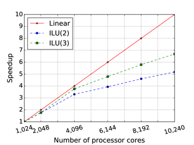
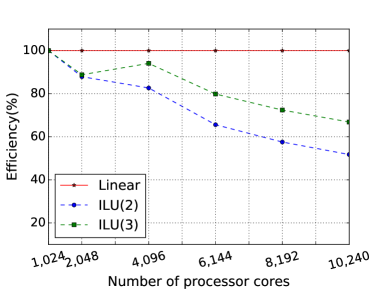
Figure 9: Speedup and parallel efficiency of the overall algorithm using up to 10,240 processor cores. Right: speedup; left: parallel efficiency.

To further understand the algorithm performance, we summarize the compute times spent on the individual components of the algorithm in Table 7. Different components of the algorithm have different properties so that the speedup and parallel efficiency are different. Some components, such as the Jacobian and function evaluations, are perfectly scalable, and other component, for example preconditioner setup, is difficult to scale. For convenience, let us introduce the notations used in Table 7. “KSPSolve” is the compute time spent on the linear solver, “KSPSetUp” denotes the time on the linear solver setup, “PCSetUp” represents the time for the preconditioner setup, “PCApply” is the time used in the application of the preconditioner, “FuncEval” denotes the function evaluation time, and “JacEval” is the time spent on the Jacobian evaluation. Data for ILU(2) and ILU(3) are separated by a dashed line, and the results for different processor counts are separated by a solid line. The record consists of two rows; the second row is the actual compute time of the individual component and the first row is the proportion of the total compute time in percentage. The total compute time, “T”, is composed of the time spent on the linear solver, the function evaluation and the Jacobian evaluation, and the preconditioner setup and application is part of the linear solver.

Table 7: Strong scalability of the algorithm components with up to 1,0240 processor cores. Newton-Krylov-Schwarz is used to solve a nonlinear system of equations with 90,551,052 unknowns.

$np$	subsolver	T	KSPSolve	KSPSetUp	PCSetUP	PCApply	FuncEval	JacEval
–	–	100%	61%	0.1%	6%	51%	5%	35%
1,024	ILU(2)	1587.5	960.8	1.5	93	827.4	73.1	561.2
–	–	100%	72%	0.1%	8%	62%	3%	25%
1,024	ILU(3)	2382.6	1716.2	2.4	199.7	1476.8	76.6	596.5
–	–	100%	64%	0.2%	12%	50%	4%	33%
2,048	ILU(2)	903.4	574.6	1.5	107.6	447.3	37.5	298.3
–	–	100%	72%	0.1%	9%	61%	3%	26%
2,048	ILU(3)	1341.9	962.2	1.6	126.1	817	42.4	345.3
–	–	100%	64%	0.2%	12%	50%	4%	32%
4,096	ILU(2)	480.3	309.5	0.9	58.6	241.9	19.7	154.4
–	–	100%	72%	0.1%	10%	61%	3%	25%
4,096	ILU(3)	633.3	457.3	0.9	62.1	387.5	19.9	159.1
–	–	100%	72%	0.2%	20%	49%	3%	26%
6,144	ILU(2)	403.5	289.1	0.7	81.9	197.9	12.9	104.1
–	–	100%	77%	0.1%	19%	57%	3%	21%
6,144	ILU(3)	497.5	383.4	0.7	93.6	284.3	13	103.8
–	–	100%	74%	0.1%	25%	47%	3%	24%
8,192	ILU(2)	344.9	254.7	0.5	86.8	161.8	10	83
–	–	100%	79%	0.1%	21%	47%	2%	20%
8,192	ILU(2)	411.5	324	0.5	88	230.9	9.8	80.3
–	–	100%	76%	0.1%	29%	46%	3%	22%
10,240	ILU(2)	306.8	233.5	0.5	87.6	140.8	8	68
–	–	100%	79%	0.1%	24%	53%	2%	20%
10,240	ILU(3)	356.5	280.5	0.5	86.2	190.7	8.2	70.6

Theoretically, the Jacobian and function evaluation should be perfectly scalable as long as the number of linear iterations and Newton iterations does not increase much when we increase the number of processor cores. From the last and the second to the last columns of Table 7, we observe that the compute time spent on the Jacobian evaluation and the function evaluation are almost halved when we double the number of processor cores, which indicates that both the function evaluation and the Jacobian evaluation are ideally scalable. This phenomenon is also observed from Fig. 10 and 11.

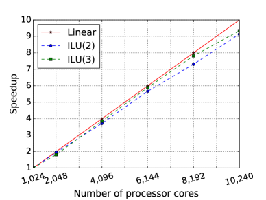
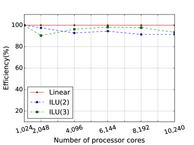
Figure 10: Speedup and parallel efficiency of the function evaluation using up to 10,240 processor cores. Right: speedup; left: parallel efficiency.

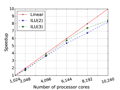
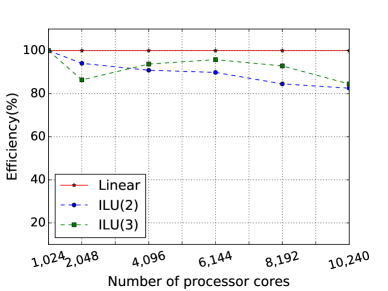
Figure 11: Speedup and parallel efficiency of the overall algorithm using up to 10,240 processor cores. Right: speedup; left: parallel efficiency.

Among the algorithmic components, “KSPSolve” takes most of the compute time, that is, it takes $61\%$ of the total compute time with ILU(2) at 1,024 cores and increases to $76\%$ at 10,240 cores. Compared with the ILU(2) case, the proportion is a little more in the ILU(3) case, where $72\%$ of the total compute time is used for solving the Jacobian system when the number of processor cores is 1,240, and it is increased a little to $79\%$ for 10,240 processor cores. The speedup and parallel efficiency of the linear solver, shown in Fig 12, is similar to that of the overall algorithm because it takes most of the total compute time.

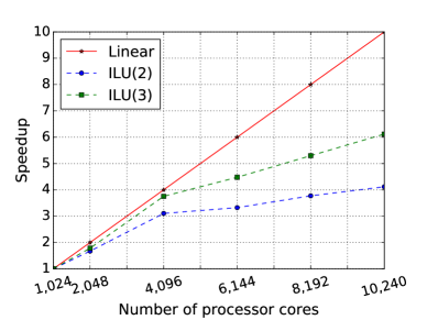
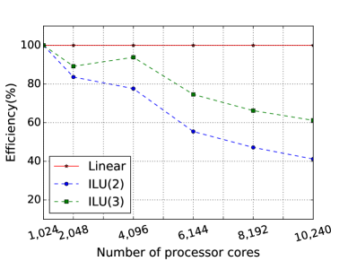
Figure 12: Speedup and parallel efficiency of the linear solver using up to 10,240 processor cores. Right: speedup; left: parallel efficiency.

The linear solver consists of the vector orthogonalization, the preconditioner setup, and the preconditioner application, especially the preconditioner setup and application take most of the linear solver time. Therefore, the design and development of the preconditoner is critical to have the overall algorithm scalable. The preconditioner setup takes less than or around $10\%$ of the total compute when the number of processor cores is less than or equal to 4,096 processor cores, and it takes up around $20\%$ when the number of processor cores is more than 4,096 but the overall algorithm still has the parallel efficiencies of $52\%$ with ILU(2) and $67\%$ with ILU(3) at 10,240 processor cores. The precondiitoner application take $50\%$ of the total compute time for all cases, and the proportion does not change with the increase of the processor count for both ILU(2) and ILU(3) indicates that preconditioner application has almost the same speedup and parallel efficiency, shown in Fig 13, as the overall algorithm. In all, all components except the precondiitoner setup are scalable so that the overall algorithm scales reasonably well with up to 10,240 processor cores.

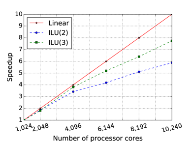
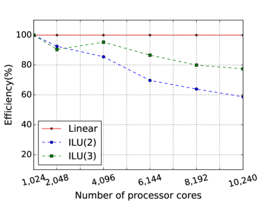
Figure 13: Speedup and parallel efficiency of the preconditioner application using up to 10,240 processor cores. Right: speedup; left: parallel efficiency.

4.8 Mesh preparation

A high quality mesh is very important for the accuracy of the simulation, and also for the rapid convergence of the iterative methods used in the simulation. In addition to high quality fluid and solid meshes, the quality of the interface mesh is also important. For arteries with a small number of branches, good meshes are quite easy to generate, but when the computational domain is complex, such as the complete pulmonary artery, the FSI mesh generation is nontrivial and often the mesh obtained from the meshing tools such as ANSYS [20] doesn’t have the required quality. This is especially the true for the mesh at the fluid-structure interface. More precisely speaking, the interface mesh produced by the software sometimes contains elements that belong to the interior of the fluid or the solid domain. To overcome this difficulty, we introduce an interface mesh reconstruction scheme that removes wrong interface elements and creates a new interface mesh by transversing through all fluid mesh elements. The basic idea of the algorithm is that we walk through the fluid mesh, and for each tetrahedron element, we mark one of its surface triangles as an interface element if the triangle is shared by a solid element. Let $\Omega_{h,s}=\{K_{s}\}$ and $\Omega_{h,f}=\{K_{f}\}$ be the solid and fluid meshes consisting of non-overlapping tetrahedrons. Each fluid element is composed of four surface triangles, $\{T_{f}\}$. $S_{I}$ represents the interface mesh constructed from the solid and fluid volume meshes. The detailed method is summarized in Algorithm 1. A sample interface mesh is shown in Fig. 14.

Algorithm 1 Interface Mesh Reconstructing

1:$S_{I}=\{\}$

2:for $K_{f}\in\Omega_{h,f}$ do

3:     for $T_{f}\in K_{f}$ do

4:         Find the neighboring element, $K$, that shares $T_{f}$ with $K_{f}$

5:         if $K\in\Omega_{h,s}$ then

6:              $S_{I}=S_{I}+T_{f}$

7:         end if

8:     end for

9:end for

10:return $S_{I}$

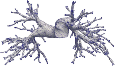
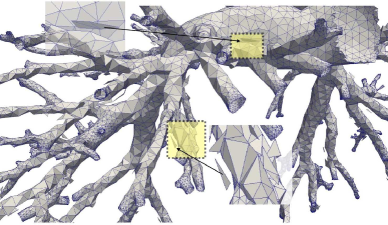
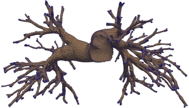
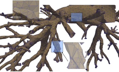
Figure 14: Interface meshes. Top: invalid interface containing several interior elements, bottom: the reconstructed interface mesh where the illegal elements have been removed.

In Fig. 14, it is easy to see that there are several illegal interface elements that are floating; i.e., not attached to the interface. This is observed from the top right picture, and it is repaired using Algorithm 1, and the new interface mesh is shown in the bottom left picture where the illegal interface elements are removed. A valid FSI mesh is shown in Fig. 15.

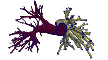
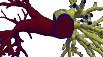
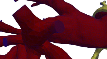
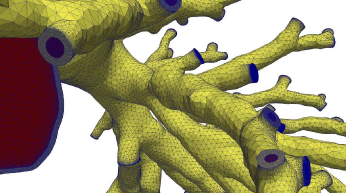
Figure 15: A sample mesh for fluid-structure interaction simulation.

5 Final remarks

Numerical simulation of blood flows in a compliant pulmonary artery is challenging because of the highly nonlinear nature of mathematical models for the fluid flow and the arterial wall, the complex configurations of the arterial network, and also the size of the discretized problem. In this paper, we developed a highly parallel algorithm for solving the monolithically coupled fluid-structure system on a supercomputer with more than 10,000 processors. Using this technology, the simulation of unsteady blood flows in a full three-dimensional, patient-specific pulmonary artery can be obtained in less than a few hours. In order to apply the techniques for clinical applications, more works are needed, such as more realistic boundary conditions, and materials parameters.

References

- [1] Wang H, Naghavi M, Allen C, Barber R, Carter A, Casey D, Charlson F, Chen A, Coates M, Coggeshall M, et al.. Global, regional, and national life expectancy, all-cause mortality, and cause-specific mortality for 249 causes of death, 1980–2015: a systematic analysis for the Global Burden of Disease Study 2015. The Lancet 2016; 388(10053):1459–1544.
- [2] Kheyfets VO, Rios L, Smith T, Schroeder T, Mueller J, Murali S, Lasorda D, Zikos A, Spotti J, Reilly Jr JJ, et al.. Patient-specific computational modeling of blood flow in the pulmonary arterial circulation. Comput. Methods Programs Biomed. 2015; 120(2):88–101.
- [3] Crosetto P, Reymond P, Deparis S, Kontaxakis D, Stergiopulos N, Quarteroni A. Fluid–structure interaction simulation of aortic blood flow. Comput. Fluids 2011; 43(1):46–57.
- [4] Verdugo F, Roth CJ, Yoshihara L, Wall WA. Efficient solvers for coupled models in respiratory mechanics. Int. J. Numer. Methods Biomed. Eng. 2017; 33(2).
- [5] Farhat C, Lesoinne M, Le Tallec P. Load and motion transfer algorithms for fluid/structure interaction problems with non-matching discrete interfaces: Momentum and energy conservation, optimal discretization and application to aeroelasticity. Comput. Methods Appl. Mech. Eng. 1998; 157(1-2):95–114.
- [6] Kong F, Cai XC. Scalability study of an implicit solver for coupled fluid-structure interaction problems on unstructured meshes in 3D. Int. J. High Perform. Comput. Appl. 2018; 32(2):207–219.
- [7] Kong F, Cai XC. A scalable nonlinear fluid–structure interaction solver based on a Schwarz preconditioner with isogeometric unstructured coarse spaces in 3D. J. Comput. Phys. 2017; 340:498–518.
- [8] Bazilevs Y, Calo VM, Zhang Y, Hughes TJ. Isogeometric fluid–structure interaction analysis with applications to arterial blood flow. Comput. Mech. 2006; 38(4-5):310–322.
- [9] Farhat C, Van der Zee KG, Geuzaine P. Provably second-order time-accurate loosely-coupled solution algorithms for transient nonlinear computational aeroelasticity. Comput. Methods Appl. Mech. Eng. 2006; 195(17-18):1973–2001.
- [10] Kong F, Wang Y, Schunert S, Peterson JW, Permann CJ, Andrš D, Martineau RC. A fully coupled two-level Schwarz preconditioner based on smoothed aggregation for the transient multigroup neutron diffusion equations. Numer. Linear Algebra Appl. 2018; https://doi.org/10.1002/nla.2162.
- [11] Causin P, Gerbeau JF, Nobile F. Added-mass effect in the design of partitioned algorithms for fluid–structure problems. Comput. Methods Appl. Mech. Eng. 2005; 194(42-44):4506–4527.
- [12] Souli M, Ouahsine A, Lewin L. ALE formulation for fluid–structure interaction problems. Comput. Methods Appl. Mech. Eng. 2000; 190(5-7):659–675.
- [13] Spilker RL, Feinstein JA, Parker DW, Reddy VM, Taylor CA. Morphometry-based impedance boundary conditions for patient-specific modeling of blood flow in pulmonary arteries. Ann. Biomed. Eng. 2007; 35(4):546–559.
- [14] Tang BT, Fonte TA, Chan FP, Tsao PS, Feinstein JA, Taylor CA. Three-dimensional hemodynamics in the human pulmonary arteries under resting and exercise conditions. Ann. Biomed. Eng. 2011; 39(1):347–358.
- [15] Qureshi MU, Vaughan GD, Sainsbury C, Johnson M, Peskin CS, Olufsen MS, Hill N. Numerical simulation of blood flow and pressure drop in the pulmonary arterial and venous circulation. Biomech. Model. Mechanobiol. 2014; 13(5):1137–1154.
- [16] Su Z, Hunter KS, Shandas R. Impact of pulmonary vascular stiffness and vasodilator treatment in pediatric pulmonary hypertension: 21 patient-specific fluid–structure interaction studies. Comput. Methods Programs Biomed. 2012; 108(2):617–628.
- [17] Hunter KS, Lanning CJ, Chen SYJ, Zhang Y, Garg R, Ivy DD, Shandas R. Simulations of congenital septal defect closure and reactivity testing in patient-specific models of the pediatric pulmonary vasculature: a 3D numerical study with fluid-structure interaction. J. Biomech. Eng. 2006; 128(4):564–572.
- [18] CFD-ACE+. https://www.esi-group.com 2017; .
- [19] Yang X, Liu Y, Yang J. Fluid-structure interaction in a pulmonary arterial bifurcation. J. Biomech. 2007; 40(12):2694–2699.
- [20] ANSYS. http://www.ansys.com 2017; .
- [21] Wu Y, Cai XC. A fully implicit domain decomposition based ALE framework for three-dimensional fluid–structure interaction with application in blood flow computation. J. Comput. Phys. 2014; 258:524–537.
- [22] Kong F. A Parallel Implicit Fluid-structure Interaction Solver with Isogeometric Coarse Spaces for 3D Unstructured Mesh Problems with Complex Geometry. PhD Thesis, University of Colorado Boulder 2016.
- [23] Kong F, Kheyfets V, Finol E, Cai XC. An efficient parallel simulation of unsteady blood flows in patient-specific pulmonary artery. Int. J. Numer. Methods Biomed. Eng. 2018; https://doi.org/10.1002/cnm.2952.
- [24] Kong F, Cai XC. A highly scalable multilevel Schwarz method with boundary geometry preserving coarse spaces for 3D elasticity problems on domains with complex geometry. SIAM J. Sci. Comput. 2016; 38(2):C73–C95.
- [25] Howell P, Kozyreff G, Ockendon J. Applied Solid Mechanics, vol. 43. Cambridge University Press, 2009.
- [26] Taylor CA, Hughes TJ, Zarins CK. Finite element modeling of blood flow in arteries. Comput. Methods Appl. Mech. Eng. 1998; 158(1-2):155–196.
- [27] Whiting CH, Jansen KE. A stabilized finite element method for the incompressible Navier-Stokes equations using a hierarchical basis. Int. J. Numer. Methods Fluids 2001; 35(1):93–116.
- [28] Barker AT, Cai XC. Scalable parallel methods for monolithic coupling in fluid-structure interaction with application to blood flow modeling. J. Comput. Phys. 2010; 229(3):642–659.
- [29] Dembo RS, Eisenstat SC, Steihaug T. Inexact Newton methods. SIAM J. Numer. Anal. 1982; 19(2):400–408.
- [30] Saad Y. Iterative Methods for Sparse Linear Systems, vol. 82. SIAM, 2003.
- [31] Smith B, Bjorstad P, Gropp W. Domain Decomposition: Parallel Multilevel Methods for Elliptic Partial Differential Equations. Cambridge University Press, 2004.
- [32] Dennis Jr JE, Schnabel RB. Numerical Methods for Unconstrained Optimization and Nonlinear Equations, vol. 16. SIAM, 1996.
- [33] Toselli A, Widlund O. Domain Decomposition Methods: Algorithms and Theory, vol. 34. Springer Science & Business Media, 2006.
- [34] Karypis G, Schloegel K, Kumar V. Parmetis: Parallel Graph Partitioning and Sparse Matrix Ordering Library. Technical Report, Department of Computer Science, University of Minnesota 1997.
- [35] Balay S, Abhyankar S, Adams MF, Brown J, Brune P, Buschelman K, Dalcin L, Eijkhout V, Gropp WD, Kaushik D, et al.. PETSc Users Manual. Technical Report ANL-95/11 - Revision 3.9, Argonne National Laboratory 2018. URL http://www.mcs.anl.gov/petsc.