Sensitivity of the Geomagnetic Octupole to a Stably Stratified Layer in the Earth’s Core

Abstract

Current “Earth-like” numerical dynamo simulations are able to reproduce many characteristics of the observed geomagnetic field. One notable exception is the geomagnetic octupolar component. Here we investigate whether a stably stratified layer at the top of the core, a missing ingredient in standard dynamo simulations, can explain the observed geomagnetic octupole. Through numerical simulations, we find that the existence of a stable layer has significant influence on the octupolar-to-dipolar ratio of the magnetic field. Particularly, we find that a 60 km stable layer with relatively strong stability or a 130 km layer with relatively weak stability are compatible with the observations, but a 350 km stable layer, as suggested by recent seismological evidence, is not compatible with Earth’s octupole field over the past 10,000 years.

Geophysical Research Letter

Department of Earth and Planetary Science, Johns Hopkins University, Baltimore, MD 21218, USA. Johns Hopkins University, Applied Physics Laboratory, Laurel, MD 20732, USA.

Chi Yancyan10@jhu.edu

Most standard Earth-like numerical dynamo simulations cannot reproduce the geomagnetic octupolar component from the past 10,000 years.

We implement a stably-stratified layer at the top of the core in dynamo models to determine the effects on the magnetic octupole.

We find that specific ranges of stable layer thickness and stability are needed to match geomagnetic observations.

1 Introduction

The geomagnetic field is generated through dynamo action operating in Earth’s liquid outer core, where convection is driven by thermal and compositional buoyancy forces as Earth slowly cools and the inner core solidifies. Archeomagnetic and paleomagnetic data demonstrate that Earth’s field is axially-dipolar dominated on long timescales and exhibits variability on various timescales including westward drift, excursions and aperiodic reversals. Numerical simulations of dynamo action are used to investigate the mechanism responsible for generating Earth’s magnetic field. Comparing the results of these simulations to observations of the present and past geomagnetic field provides vital information on processes occurring in Earth’s deep interior. Geodynamo models aim to reproduce the salient features of the geomagnetic field including the dipole dominance, spatial power spectrum and temporal characteristics of the variability. Researchers have proposed quantitative criteria for determining whether a simulated field is “Earth-like” and determined regions of parameter space where such fields occur (Christensen et al., 2010; Davies $\&$ Constable, 2014). Models in this parameter space are believed to provide the best insights into Earth’s dynamo processes.

However, one large-scale field characteristic that many Earth-like models cannot reproduce is the octupolar component of the magnetic field (Figure 1). Here we use Gauss coefficients to represent the different modes of the magnetic field morphology. Outside the fluid core, where the magnetic field $\mathbf{B}$ can be represented as the gradient of a scalar potential $V$, the Gauss coefficients are defined by the expression

$$V(r,\theta,\phi)=r_{e}\sum^{\infty}_{l=1}\sum^{l}_{m=0}[g^{m}_{l}cosm\phi+h^{m}_{l}sinm\phi]{(\frac{r_{e}}{r})}^{l+1}P^{m}_{l}(cos\theta)$$ (1)

where $r$ is radius, $\theta$ is co-latitude, $\phi$ is longitude, $r_{e}$ is the radius of Earth’s surface, $g^{m}_{l}$ and $h^{m}_{l}$ are Gauss coefficients, $l$ and $m$ are spherical harmonic degree and order, respectively, and $P^{m}_{l}(cos\theta)$ are associated Legendre polynomials. The three largest zonal signals are the dipole ($g^{0}_{1}$), quadrupole ($g^{0}_{2}$) and octupole ($g^{0}_{3}$). Following previous studies, we scale the octupole and quadrupole components to the dipole component ($g^{0}_{3}/g^{0}_{1}$ and $g^{0}_{2}/g^{0}_{1}$) for comparison. A standard Earth-like model tends to produce an octupolar-to-dipolar ratio ($g^{0}_{3}/g^{0}_{1}$) that is always positive and larger than observational values over the past 10,000 years. This discrepancy between a standard model and the paleomagnetic model suggests that another ingredient may be necessary in the models to properly simulate Earth’s dynamo processes.

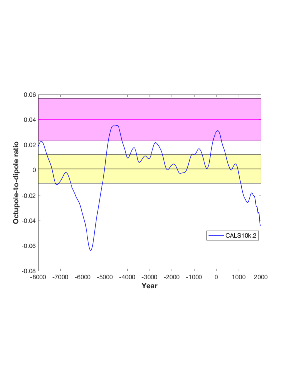
Figure 1: The magnetic octupole-to-dipole ratio for paleomagnetic observations from the past 10,000 years from CALS10k.2 (Constable et al.,, 2016) and for an Earth-like dynamo model that does not include a stable layer (Model 0 of Table 1). The simulation time is re-dimensionalized through the magnetic diffusion time scale $d^{2}/\eta$ to have the same time span as in the CALS10k.2 model. The magenta line gives the time-averaged value from the model and the shaded magenta region represents the standard deviation about the average. The observational values are shown in the solid blue line with the black line representing the average and the shaded yellow region representing the standard deviation about the average.

Here we investigate whether a stably stratified layer at the top of Earth’s core could be that ingredient. The presence of such a layer has long been proposed based on evidence from seismology (Tanaka $\&$ Hamaguchi, 1993) and geomagnetic secular variation (Braginsky, 1993, 1999). However, there is disagreement on the thickness and stability of this layer; properties which depend on the stable layer’s origins. Recent seismological evidence suggests the layer may be over 300 km thick (Tang et al., 2015; Kaneshima, 2018)) whereas secular variation studies suggest a thickness between $60-140$ km (Gubbins, 2007; Buffett, 2014)). Proposed origins for such a layer include a sub-adiabatic temperature gradient in the upper core due to its high thermal conductivity, producing a stable layer with thickness that may range from $\sim 100$ km (Lister $\&$ Buffett, 1998) to $\sim 740$ km (Gubbins et al., 2015); compositional layering due to light element expulsion from inner core crystallization, resulting in a $\sim 250$ km thick layer (Helffrich, 2013); barodiffusion in the core, with a $\sim 100$ km thick layer (Gubbins $\&$ Davies, 2012); or a relic of merging cores from giant impacts early in Earth’s history, with a $\sim 300$ km thick layer (Landeau et al., 2016).

In this study we use numerical dynamo simulations to evaluate the effects of a stably stratified layer at the top of Earth’s outer core on the resulting geomagnetic octupole. Details of the numerical methods can be found in Section 2, results in Section 3, discussions in Section 4, and conclusions in Section 5.

2 Numerical Methods

We use the numerical dynamo model mMoSST (Jiang $\&$ Kuang, 2008) to solve the coupled equations governing dynamo action in a fluid, electrically conducting, rotating outer core surrounding a solid, electrically conducting inner core. This model has been shown to reproduce benchmark results (Christensen et al., 2001). Further details on the relevant dynamo equations, non-dimensional parameters and the numerical method can be found in Kuang $\&$ Bloxham (1999) and Jiang $\&$ Kuang (2008). We additionally implement a stably stratified layer at the top of the core, where the layer stability is maintained through the background co-density gradient, in a similar manner as previous dynamo studies (e.g. Stanley $\&$ Bloxham, 2004; Stanley $\&$ Mohammadi, 2008; Christensen $\&$ Wicht, 2008). Further details on the non-dimensional parameters, model equations and implementation of stratification can be found in the supplementary material.

Due to numerical constraints, dynamo simulations cannot operate with realistic Earth-like parameters. However, scaling laws can be used to determine combinations of computationally attainable parameters that can produce dynamo generation with Earth-like characteristics. Christensen et al. (2010) proposed conditions for an Earth-like dynamo model by defining quantitative criteria evaluating the level of agreement of the output from a numerical simulation with observed properties of the geomagnetic field morphology. We adopt their $\chi^{2}$ criterion, which is composed of four separate quantities, to evaluate the performance of our models. These four quantities are: (1) the ratio of the power in the axial dipole component to the power in the rest of the magnetic field, (2) the ratio of the power in the equatorially antisymmetric and symmetric magnetic field, (3) the ratio of the power in zonal and non-zonal non-dipole magnetic field, and (4) the concentration factor of magnetic flux at the core surface.

For this study, we consider model C1-4* from Davies $\&$ Constable (2014), which satisfies the $\chi^{2}$ criterion but does not reproduce the observed $g^{0}_{3}/g^{0}_{1}$ ratio (Figure 1). We add stable layers of different thicknesses, i.e. 60 km, 130 km and 350 km, and strength of stratification to this model to determine whether it is possible to match both the $\chi^{2}$ criterion and the $g^{0}_{3}/g^{0}_{1}$ ratio. We also examine a case with no stable layer for comparison. Numerical simulation details are listed in Table 1. We use the Boussinesq approximation and apply co-density boundary conditions of fixed buoyancy at the inner core boundary (ICB) and fixed buoyancy flux at the core mantle boundary (CMB); no-slip boundary conditions on the velocity field; and magnetic field boundary conditions at the ICB for a finite electrically conducting inner core with equal conductivity to the outer core and at the CMB for an insulating mantle. We use finite differencing in the radial direction with 58 Chebyshev collocation points. Each spherical shell is resolved in latitude and longitude using spherical harmonics with maximum degree and order $l_{max}=31,m_{max}=23$. Our models are resolved. For example, simulations with $l_{max}=50$, $m_{max}=41$ and 78 radial points produce similar power spectra from degree 1 to 31 and the power in the highest degree $l_{max}=50$ is 12 orders of magnitude smaller than the power in the lower degree $l_{max}=31$.

Table 1: Model parameters: $\Delta r$ is the thickness of the stable layer. $(N/2\Omega)^{2}$ measures the strength of the stable layer stratification where $N$ is the $Brunt-V\ddot{a}is\ddot{a}l\ddot{a}$ frequency and $\Omega$ is the angular velocity. Other non-dimensional parameters relevant to the models are held fixed at Ekman number of $E=1.2\times 10^{-4}$ , Prandtl number $Pr=1$, the magnetic Prandtl number $Pm=2$ and the modified Rayleigh number $R_{a}=8.33\times 10^{5}$ (note that the definition of these nondimensional numbers is given in the supplementary information).

Model	$\Delta r$ ($km$)	$(\frac{N}{2\Omega})^{2}$
0	0	0
1	60	[0 $\to$ 1.36]
2	130	[0 $\to$ 1.36]
3	350	[0 $\to$ 1.36]

3 Results

Figure 2 shows the $g^{0}_{3}/g^{0}_{1}$ ratio averaged over $10,000$ years for our models. Although we ran our simulations for longer than 10,000 years, we chosen a random 10,000 year window in our simulations to present results here and confirmed that other randomly-chosen 10,000-yr windows produced similar results. The historical $g^{0}_{3}/g^{0}_{1}$ ratio from paleomagnetic model CALS10k.2 is also shown in the yellow shaded region. For the control model with no stable layer, $g^{0}_{3}/g^{0}_{1}$ is constantly larger than the values in CALS10k.2 model and never produces the negative values seen in CALS10k.2 model. However, for models with a stable layer, the average $g^{0}_{3}/g^{0}_{1}$ ratio decreases as the layer stability increases for all values of stable layer thickness we investigated. The ratios tend towards an equilibrium value as $(N/2\Omega)^{2}$ increases. This suggests that once a layer has become stable enough to fully inhibit convective flows (see Figure S3), there is no further effect on the $g^{0}_{3}/g^{0}_{1}$ ratio. Examining the cases with different stable layer thicknesses demonstrates that the thicker the layer, the more $g^{0}_{3}/g^{0}_{1}$ is impacted, both in terms of average values and variations.

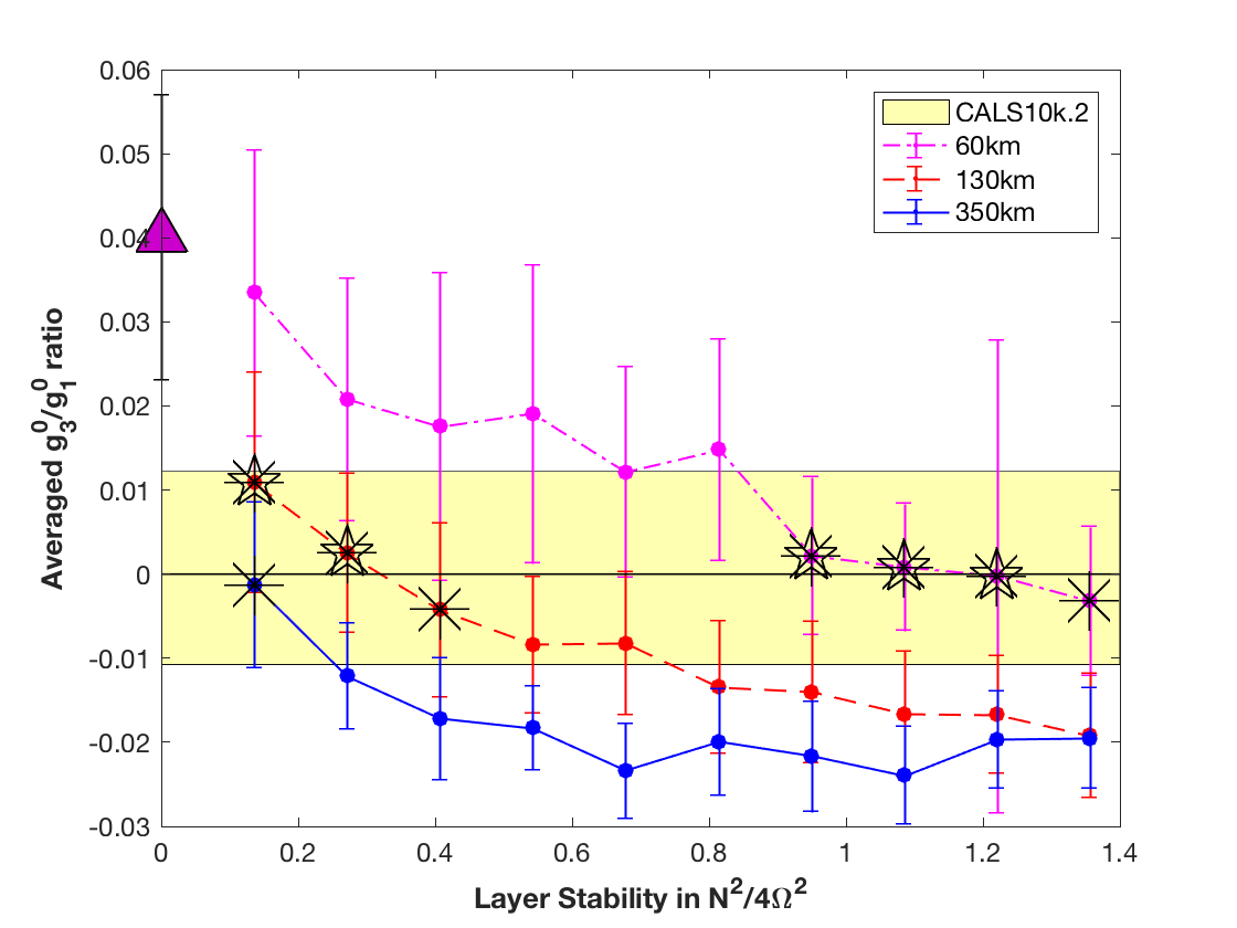
Figure 2: The $g^{0}_{3}/g^{0}_{1}$ ratio as a function of stable layer properties. The error bars show the standard deviation in time of the $g^{0}_{3}/g^{0}_{1}$ ratios about the average values given by the circles. The model represented by a triangle is the control model 0 from Table 1 with no stable layer. Asterisks mark cases producing compatible $g^{0}_{3}/g^{0}_{1}$ ratios compared to CALS10k.2 and pentagrams mark cases that also meet the criterion $\chi^{2}$.

To determine which of our models can reproduce the most Earth-like characteristics, we first exclude models that don’t produce the historical $g^{0}_{3}/g^{0}_{1}$ ratio, namely, we exclude models that don’t produce time averages that are consistent with the observations as well as models that don’t produce standard deviations that include both positive and negative values (e.g. the lack of positive $g^{0}_{3}/g^{0}_{1}$ values is why models with $\Delta r=130$ km and $(N/2\Omega)^{2}=0.54$ and $0.68$ are excluded even though their mean values are consistent with the observations). This leaves 8 cases out of 33 simulations which are marked by asterisks in Figure 2. Next we exclude models that do not meet the quantitative criterion $\chi^{2}$ from Christensen et al. (2010), leaving 5 cases marked by pentagrams in Figure 2 that comply with standards for “good” agreement ($\chi^{2}<4$) between the simulated field and the paleomagnetic model CALS10k.2 (Table S1) as well as meeting the $g^{0}_{3}/g^{0}_{1}$ ratio constraint. For visualizations of the radial magnetic field, see Figure S4(a).

We also investigated the zonal quadrupole to dipole ($g^{0}_{2}/g^{0}_{1}$) ratio in our simulations (Figure S1, S2). A standard Earth-like model without a stable layer is able to reproduce the historic values for this ratio and the addition of a stable layer in our models did not affect the ratio. Our results are therefore also consistent with observations for the quadrupolar field, although this wasn’t an issue for the standard model to begin with. The lack of dependence of the zonal quadrupole on the presence of a stable layer may be due to the fact that the zonal quadrupole belongs to a different dynamo symmetry family than the zonal octupole and dipole and is therefore generated by different convective modes.

Previous work has also demonstrated that a spatially variable CMB heat flux pattern can affect the zonal octupole component (Bloxham, 2000; Heimpel and Evans, 2013). For example, a surface spherical harmonic degree-2, order-0 ($Y^{0}_{2}$) pattern of heat flux perturbation at the CMB has been shown to result in a positive $g^{0}_{3}/g^{0}_{1}$ ratio that can better match paleomagnetic data from 250 Myr ago (Bloxham, 2000). It is thus necessary for us to examine the possible effects of the CMB heat flux variation over the past 10,000 years to disentangle the possible influences of CMB heat flux variation and the stable layer on the $g^{0}_{3}/g^{0}_{1}$ ratio. We have therefore imposed the current era’s dominant heat flux signature ($Y^{2}_{2}$ pattern) discerned from mantle tomography on the CMB in our models to investigate the effects on the $g^{0}_{3}/g^{0}_{1}$ ratio.

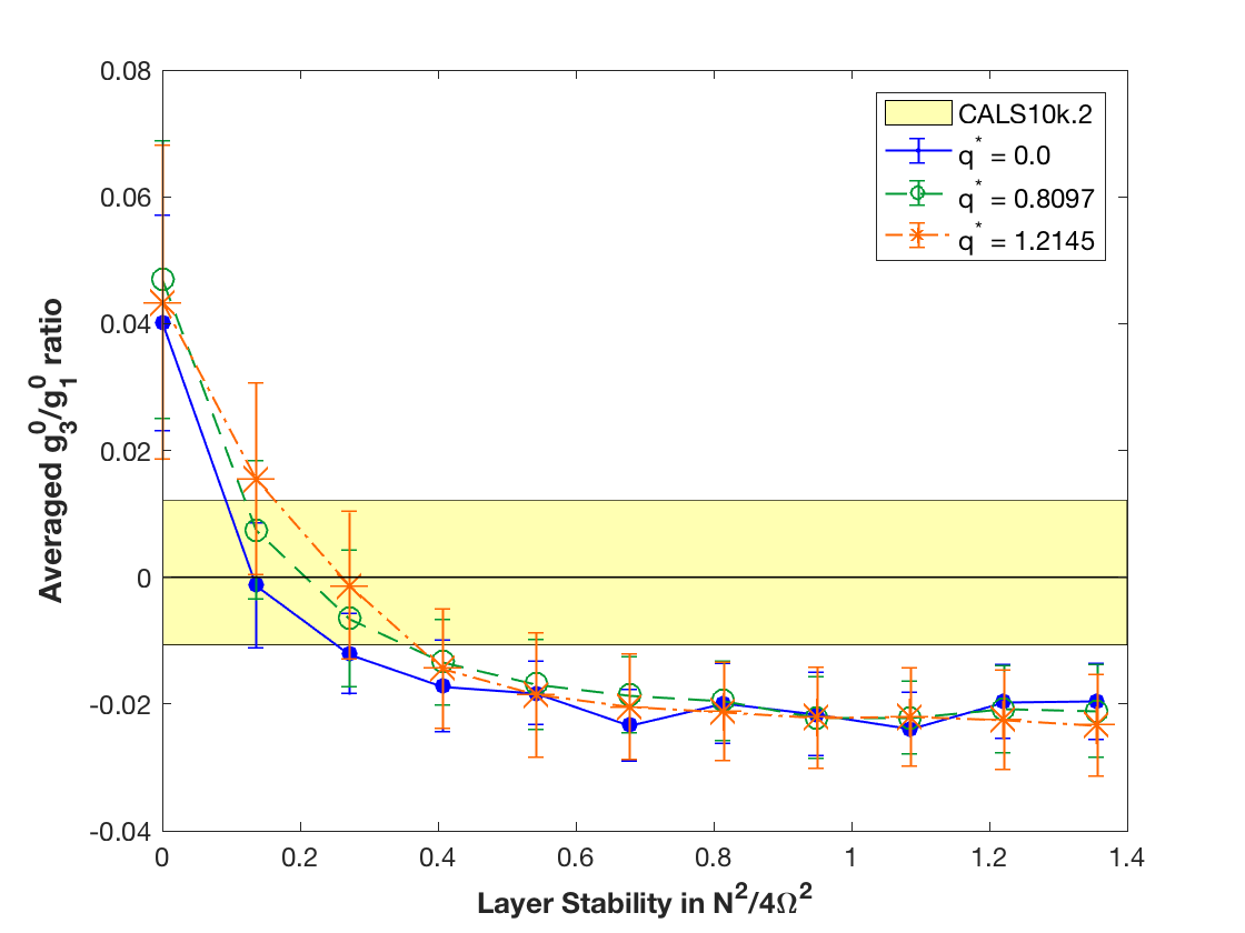
Figure 3: The sensitivity of the ratio $g^{0}_{3}/g^{0}_{1}$ to the modern day heat flux variation pattern at the CMB, for a model with a 350 km stable layer. The blue line is the same as that in Figure 2. $q^{*}$ is the ratio of the heat flux anomaly divided by twice the average heat flux at the CMB.

Figure 3 shows that: 1) when there is no stable layer, adding a $Y^{2}_{2}$ pattern of heat flux variation doesn’t change the average ratio although it causes a larger variation, as suggested previously by Bloxham (2000), and 2) a $Y^{2}_{2}$ pattern of heat flux variation did not significantly affect the $g^{0}_{3}/g^{0}_{1}$ ratio in our models. As a result, we conclude that the $g^{0}_{3}/g^{0}_{1}$ ratio is insensitive to the largest component of the modern era CMB heat flux pattern.

4 Discussion

Our study demonstrates that a stably stratified layer at the top of Earth’s core may be necessary to explain the zonal octupolar component of the geomagnetic field over the past 10,000 years. It should be noted that other magnetic models such as CHAOS-4 (Olsen et al., 2014) and gufm1 (Jackson et al., 2000) have higher spatial and temporal resolutions compared to CALS10k.2 used in this study. However, those models only cover short time periods (recent decades) and therefore represent more of a snapshot of core processes making it unclear how representative they are of longer-term behavior. We wanted to compare average behavior on longer timescales and the CALS10k.2 model allowed for that. That being said, if we were instead to assume that the CHAOS-4 and gufm1 models from data over the past couple of decades was a better proxy of the average behavior of the large-scale components of the Earth’s magnetic field over the past 10,000 years, then the prediction would be for an octupole-to-dipole ratio of $-0.0453\pm 0.0002$ which is even further removed from the standard dynamo models without a stable layer than the data from the CALS10k.2 model. This would suggest that an even larger correction to the models would be needed (e.g. a thicker, more stable layer, or other new features in the model). We therefore feel we are making the conservative choice in this study by using the CALS10k.2 data as representative of average behavior over the past 10,000 years.

Almost all models with a 350 km thick stable layer fail to match the geomagnetic octupolar constraint. The exception is our model with weak layer stability $(N/2\Omega)^{2}=0.14$ but this model fails to match the Earth-like $\chi^{2}$ criterion. This suggests discrepancy with recent seismic claims (Tang et al., 2015; Kaneshima, 2018) unless the seismic observations are capturing a physical process that is not being considered in our modeling approach of the stably stratified layer, (in particular, since the models operate in a parameter regime far from that of Earth’s core.)

The reason for the stable layer’s influence on the octupolar component of the magnetic field resides in the dynamo mechanism itself. Figure 4(a) shows that there is amplified power in velocity modes $(l,m)=(3,0)$ and $(5,0)$ due to the presence of a stable layer where models with larger layer stabilities lead to stronger amplification in these zonal flows. Dynamically as the stable layer is implemented, it forces thermal wind in the outer core (e.g. see Figure S4(b)) to be concentrated into the deeper region of the outer core, which results in a strengthened signature in the zonal octupolar toroidal kinetic energy. However, future studies are needed to scale the modeled zonal flows to these flows in real Earth conditions.

Figure 4(b) shows that models with a stable layer only see amplification in the $g^{0}_{3}/g^{0}_{1}$ ratio and not other magnetic modes. The amplified octupolar zonal flow can lead to creation of the magnetic octupole field through a two-step dynamo mechanism described with the Bullard $\&$ Gellman (1954) formalism as:
Step 1: ($T^{0}_{3}S^{1}_{2}T^{1}_{1}$)
Step 2: ($S^{1}_{2}T^{1}_{1}S^{0}_{3}$)
Step 1 is described by an Adams-Gaunt integral which involves the octupolar zonal flow ($T^{0}_{3}$) acting on the poloidal magnetic field ($S^{1}_{2}$) to generate a toroidal magnetic field ($T^{1}_{1}$). Step 2 is described by an Elsasser integral where a poloidal flow ($S^{1}_{2}$) acts on the toroidal magnetic field ($T^{1}_{1}$) which was generated in Step 1 to generate the new magnetic zonal poloidal octupole field ($S^{0}_{3}$) that is observed. Similar to the above two-step dynamo mechanism, there are other paths leading to the creation of the magnetic octupole field through the amplified zonal flow in degree 5.

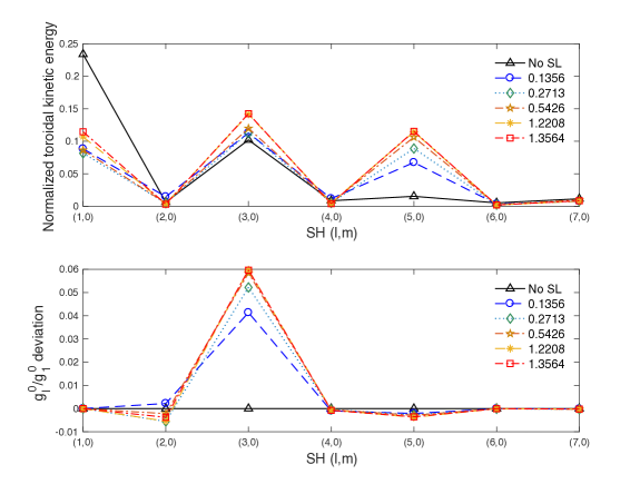
Figure 4: (a) Normalized toroidal kinetic energy as a function of zonal spherical harmonic mode and (b) Deviation of the $g^{0}_{l}/g^{0}_{1}$ ratio in the 350 km case with different stratification $(N/2\Omega)^{2}$ values, averaged over 1 magnetic diffusion time. Both x axes list the sequential zonal spherical harmonic (SH) degree, the y axis in (a) shows the fraction of the toroidal kinetic energy of a single mode whereas the y axis in (b) shows the deviation of the $g^{0}_{l}/g^{0}_{1}$ in that model compared to the $g^{0}_{l}/g^{0}_{1}$ value without a stable layer (SL).

A recent geodynamo study investigating partially stratified regions, where convection can occur locally in a stable layer due to strong thermal influences from the CMB, also found that the octupolar field is affected by the presence of a stable layer. However, they found the $g^{0}_{3}/g^{0}_{1}$ ratio increased with layer stability and always produced a positive ratio (Olson et al., 2017). Their results would therefore not be consistent with observations, although it was not the purpose of that study to match observations. The reason for the differences between our studies is likely related to the fact that they were performed in different parameter regimes. This demonstrates that the effects we observe may be limited to the specific scenario appropriate to an Earth-like dynamo regime.

The model with 130 km stable layer and $(N/2\Omega)^{2}=0.27$ in this study is similar to the result in Buffett (2014) with a 140 km layer and $(N/2\Omega)^{2}\approx 0.26$. However, the level of stratification investigated here is smaller than some previous predictions for what is expected in Earth’s stable layer. For example, the Gubbins $\&$ Davies (2012) barodiffusion model has $(N/2\Omega)^{2}$ ranging from 100 $\sim$ 400. However, the flattening of the $g^{0}_{3}/g^{0}_{1}$ ratios in our results (e.g. in Figure 2) suggests that further increasing the stratification in our models would not significantly affect the results. By this point, the layer is fully stratified with extremely small radial motions (see Figure S3). This suggests that there is no entrainment by the underlying convection into the stable region.

It is worth noting that a stably stratified layer might not be the only mechanism affecting the magnetic octupole. For example, Bloxham (2000) found that the $Y^{0}_{2}$ CMB heat flux variation pattern from 250 Ma increases the $g^{0}_{3}/g^{0}_{1}$ ratio compared to a model with no CMB heat flux variations. Modern day values of $Y^{0}_{2}$ may be quite small (e.g. Zhang $\&$ Zhong, 2011) and hence they may not significantly affect the $g^{0}_{3}/g^{0}_{1}$ ratio. However, if they are somewhat comparable to the $Y^{2}_{2}$ amplitude (as suggested in some seismic studies) then the Bloxham (2000) study suggests they would actually work to increase the $g^{0}_{3}/g^{0}_{1}$ ratio compared to a scenario with no $Y^{0}_{2}$ heat flux pattern. This could exacerbate the issue of matching the $g^{0}_{3}/g^{0}_{1}$ observations with dynamo models and would suggest that an even stronger or thicker stable layer may be needed. In addition, there are previously published dynamo models that do match the $\chi^{2}$ criterion and the $g^{0}_{3}/g^{0}_{1}$ ratio for particular parameter choices. For example, a previous study by Davies et al. (2008) captures the modern-day average $g^{0}_{3}/g^{0}_{1}$ ratio in a model with no stable layer, but in a low Rayleigh number regime with relatively large lateral CMB heat flux perturbations that may not be Earth-like. Furthermore, Landeau et al. (2017) finds that the $g^{0}_{3}/g^{0}_{1}$ ratio may also depend on inner core size. That study implemented different buoyancy conditions relevant to various potential thermal histories for the inner core and showed that the $g^{0}_{3}/g^{0}_{1}$ ratio decreases as the inner core grows through time reaching values similar to present day observations for present day inner core sizes. These studies demonstrate that a stable layer may not be the only potential explanation for the present day $g^{0}_{3}/g^{0}_{1}$ ratio, but that other ingredients involving core thermal histories may contribute as well.

5 Conclusion

Our study demonstrates that a stably stratified layer at the top of Earth’s core may be necessary to explain the zonal octupolar component of the geomagnetic field over the past 10,000 years. We found that a fairly thin stable layer (60 km) needs to be relatively strongly stratified ($(N/2\Omega)^{2}\in[0.95,1.22]$) whereas a moderately thick layer (130 km) needs to be more weakly stratified ($(N/2\Omega)^{2}\in[0.14,0.27]$). Our model with a 350 km thick stable layer could not match the geomagnetic zonal octupolar constraint and the Earth-like $\chi^{2}$ criterion.