Dynamic slip wall model for large-eddy simulation

Abstract

Wall modelling in large-eddy simulation (LES) is necessary to overcome the prohibitive near-wall resolution requirements in high-Reynolds-number turbulent flows. Most existing wall models rely on assumptions about the state of the boundary layer and require a priori prescription of tunable coefficients. They also impose the predicted wall stress by replacing the no-slip boundary condition at the wall with a Neumann boundary condition in the wall-parallel directions while maintaining the no-transpiration condition in the wall-normal direction. In the present study, we first motivate and analyse the Robin (slip) boundary condition with transpiration (nonzero wall-normal velocity) in the context of wall-modelled LES. The effect of the slip boundary condition on the one-point statistics of the flow is investigated in LES of turbulent channel flow and flat-plate turbulent boundary layer. It is shown that the slip condition provides a framework to compensate for the deficit or excess of mean momentum at the wall. Moreover, the resulting nonzero stress at the wall alleviates the well-known problem of the wall-stress under-estimation by current subgrid-scale (SGS) models (Jiménez & Moser, 2000). Secondly, we discuss the requirements for the slip condition to be used in conjunction with wall models and derive the equation that connects the slip boundary condition with the stress at the wall. Finally, a dynamic procedure for the slip coefficients is formulated, providing a dynamic slip wall model free of a priori specified coefficients. The performance of the proposed dynamic wall model is tested in a series of LES of turbulent channel flow at varying Reynolds numbers, non-equilibrium three-dimensional transient channel flow, and zero-pressure-gradient flat-plate turbulent boundary layer. The results show that the dynamic wall model is able to accurately predict one-point turbulence statistics for various flow configurations, Reynolds numbers, and grid resolutions.

1 Introduction

The near-wall resolution requirement to accurately resolve the boundary layer in wall-bounded flows remains a pacing item in large-eddy simulation (LES) for high-Reynolds-number engineering applications. Choi & Moin (2012) estimated that the number of grid points necessary for a wall-resolved LES scales as $\Rey^{13/7}$, where $\Rey$ is the characteristic Reynolds number of the problem. The computational cost is still excessive for many practical problems, especially for external aerodynamics, despite the favourable comparison to the $\Rey^{37/14}$ scaling required for direct numerical simulation (DNS), where all the relevant scales of motion are resolved.

By modelling the near-wall flow such that only the large-scale motions in the outer region of the boundary layer are resolved, the grid-point requirement for wall-modelled LES scales at most linearly with increasing Reynolds number. Therefore, wall-modelling stands as the most feasible approach compared to wall-resolved LES or DNS. Several strategies for modelling the near-wall region have been explored in the past, and most of them are effectively applied by replacing the no-slip boundary condition in the wall-parallel directions by a Neumann condition. This fact is motivated by the observation that, with the no-slip condition, most subgrid scale models do not provide the correct stress at the wall when the near-wall layer is not resolved by the grid (Jiménez & Moser, 2000).

Examples of the most popular and well-known wall models are the traditional wall-stress models (or approximate boundary conditions), and detached eddy simulation (DES) and its variants. Approximate boundary condition models compute the wall stress using either the law of the wall (Deardorff, 1970; Schumann, 1975; Piomelli et al., 1989; Yang et al., 2015) or the Reynolds-averaged Navier-Stokes (RANS) equations (Balaras et al., 1996; Wang & Moin, 2002; Chung & Pullin, 2009; Kawai & Larsson, 2013; Park & Moin, 2014). DES (Spalart et al., 1997) combines RANS equations close to the wall and LES in the outer layer, with the interface between RANS and LES domains enforced implicitly through the change in the turbulence model. The reader is referred to Piomelli & Balaras (2002), Cabot & Moin (2000), Larsson et al. (2016), and Bose & Park (2018) for a more comprehensive review of wall-stress models and to Spalart (2009) for a review of DES.

One of the most important limitations of the models above is that they depend on pre-computed parameters and/or assume explicitly or implicitly a particular law for the mean velocity profile close to the wall. Recently this has been challenged by Bose & Moin (2014) with a dynamic slip wall model that is free of any a priori specified coefficients. In addition, the no-transpiration condition used in most wall models was replaced by a Robin boundary condition in the wall-normal direction. The present study extends the work by Bose & Moin (2014) and is divided in two parts. In the first part, we investigate the use of the slip boundary condition at the wall for the three velocity components in the context of wall-modelled LES. The motivation for the use of this boundary condition is corroborated both theoretically and through detailed a priori tests of filtered velocity fields. We then assess whether this condition is physically advantageous compared to other boundary conditions when the LES grid resolution is insufficient to accurately resolve the near-wall region. Additionally, sensitivities of the slip boundary condition with respect to Reynolds number, grid resolution, and SGS model in actual LES are explored. In the second part of the paper, we discuss the requirements for constructing wall models based on the slip condition and propose a dynamic procedure independent of any a priori tunable parameters, consistent with the slip boundary condition, and based on the invariance of wall stress under test filtering.

The paper is organised as follows. In section 2, we present and motivate the suitability of the slip boundary condition for LES by considering the behaviour of the filtered velocities at the wall. A priori testing is performed on filtered DNS data to test the validity of the analysis. In section 3, we perform a set of turbulent channel LES with the slip boundary condition and study the effect of the slip parameters, choice of SGS model, grid resolution, and Reynolds number on the one-point statistics such as the mean and root-mean-squared (rms) velocity profiles. A dynamic procedure is presented in section 4, and its performance is evaluated in section 5 for LES of two-dimensional and non-equilibrium three-dimensional transient turbulent channel flows, and zero-pressure-gradient flat-plate turbulent boundary layer. Finally, conclusions are offered in section 6.

2 Slip boundary condition with transpiration

We define the slip boundary condition with transpiration as

$$\bar{u}_{i}|_{w}=l_{i}\left.\frac{\partial\bar{u}_{i}}{\partial n}\right|_{w}+v_{i},\quad i=1,2,3,$$ (1)

where repeated indices do not imply summation. The indices $i=1,2,3$ denote the streamwise, wall-normal, and spanwise spatial directions represented by $x_{1},x_{2}$ and $x_{3}$, respectively, $u_{i}$ are the flow velocities, $\bar{(\cdot)}$ is the resolved LES field (or filter operation), $n$ is the wall-normal direction, and $(\cdot)|_{w}$ indicates quantities evaluated at the wall. The grid or filter size will be denoted as $\Delta_{i}$ for the respective directions. We define $l_{i}$ to be the slip lengths and $v_{i}$ the slip velocities. In general, both the slip lengths and velocities are functions of space and time. A sketch of the slip boundary condition for a flat wall is given in figure 1.

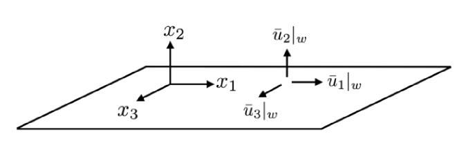
Figure 1: Sketch of the slip boundary condition with transpiration ($\bar{u}_{2}|_{w}\neq 0$) for a flat wall.

In this section, we provide theoretical motivation for the slip boundary condition in the context of filtered velocity components and inspect the validity of (1) using a priori testing of filtered DNS data. The physical implications of the slip lengths are also investigated in terms of the mean velocity profile and rms velocity fluctuations. Some preliminary results of this section can be found in Bae et al. (2016).

2.1 Theoretical motivation

Let us consider a wall-bounded flow. For the Navier-Stokes equations, the velocity at the wall is given by the no-slip boundary condition (Stokes et al., 1901)

$$\left.u_{i}\right|_{w}=0,\quad i=1,2,3.$$ (2)

If we interpret LES as the solution of the filtered Navier-Stokes equations (Leonard, 1975), the filtering operation in the wall-normal direction will result, in general, in non-zero velocities at the wall. For wall-resolved LES, where the effective filter size near the wall is small, $\left.\bar{u}_{i}\right|_{w}$ can still be approximated by the no-slip boundary condition (Ghosal & Moin, 1995). However, when the filter size is large or the near wall resolution is coarse, such as in wall-modelled LES, a modified wall boundary condition different from the usual no-slip is required for the three velocity components. Consider a one-dimensional symmetric filter kernel $\mathcal{G}(\chi)$ with nonzero filter size $\Delta_{\mathcal{G}}$ defined by its second moment

$$\Delta_{\mathcal{G}}^{2}=\int_{-\infty}^{\infty}\mathcal{G}({\chi^{\prime}}){\chi^{\prime 2}}\,\mathrm{d}{\chi^{\prime}}.$$ (3)

Then, far from the wall ($x_{2}\gg\Delta_{\mathcal{G}}$), where $x_{2}=0$ is the location of the wall, the filtered velocity field can be computed as

$$\bar{u}_{i}(\boldsymbol{x})=\int_{-\infty}^{\infty}\int_{-\infty}^{\infty}\int_{-\infty}^{\infty}\mathcal{G}(-{x_{1}}+{\chi_{1}^{\prime}})\mathcal{G}(-{x_{2}}+{\chi_{2}^{\prime}})\mathcal{G}(-{x_{3}}+{\chi_{3}^{\prime}})u_{i}(\boldsymbol{\chi^{\prime}})\,\mathrm{d}\boldsymbol{\chi^{\prime}},$$ (4)

where $\boldsymbol{x}=(x_{1},x_{2},x_{3})$ and $\boldsymbol{\chi^{\prime}}=(\chi_{1}^{\prime},\chi_{2}^{\prime},\chi_{3}^{\prime})$. However, in the near-wall region, the filter kernel in the wall-normal direction has a functional dependence on the wall-normal distance, which becomes prevalent for $x_{2}\rightarrow 0$, as depicted in figure 2. The new filter operator restricted by the wall then becomes

$$\bar{u}_{i}(\boldsymbol{x})=\int_{-\infty}^{\infty}\int_{0}^{\infty}\int_{-\infty}^{\infty}\mathcal{G}(-{x_{1}}+{\chi_{1}^{\prime}})\mathcal{G}^{*}(-{x_{2}}+{\chi_{2}^{\prime}};x_{2})\mathcal{G}(-{x_{3}}+{\chi_{3}^{\prime}})u_{i}(\boldsymbol{\chi^{\prime}})\,\mathrm{d}\boldsymbol{\chi^{\prime}}$$ (5)

where

$$\mathcal{G}^{*}(\chi;x_{2})=\frac{\mathcal{G}(\chi)}{\int_{-x_{2}}^{\infty}\mathcal{G}(\varphi)\,\mathrm{d}\varphi}$$ (6)

is the effective (rescaled) kernel at a wall-normal distance $x_{2}$.

Figure 2: Sketch of the change in effective kernel approaching the wall.

Assuming a no-slip boundary condition for the unfiltered velocity and approximating the velocity profile near the wall as a Taylor expansion $u_{i}(\boldsymbol{x})=\sum_{m=1}^{p}a_{m}x_{2}^{m}$, the filtered velocity can be expressed as

$$\bar{u}_{i}|_{w}=\sum_{m=1}^{p}a_{m}M_{\mathcal{G}^{*}_{0}}^{(m)},$$ (7)

where $M_{\mathcal{G}^{*}_{0}}^{(m)}$ is the $m$-th moment of $\mathcal{G}^{*}(\chi;0)$, the effective filter at the wall. From (7), it can be shown that

$$\left.\frac{\partial\bar{u}_{i}}{\partial x_{2}}\right|_{w}=\sum_{m=1}^{p}-2a_{m}\mathcal{G}(0)M_{\mathcal{G}_{0}^{*}}^{(m)}+ma_{m}M_{\mathcal{G}_{0}^{*}}^{(m-1)}.$$ (8)

Since $M_{\mathcal{G}_{0}^{*}}^{(m)}\sim\Delta_{\mathcal{G}}^{m}$ and $\mathcal{G}(0)\sim\Delta_{\mathcal{G}}^{-1}$, we can use (7) and (8) to obtain a second-order approximation of the boundary condition of the form

$$\bar{u}_{i}|_{w}=l\left.\frac{\partial\bar{u}_{i}}{\partial x_{2}}\right|_{w},$$ (9)

where $l=M_{\mathcal{G}_{0}^{*}}^{(1)}/\left(1-2\mathcal{G}(0)M_{\mathcal{G}_{0}^{*}}^{(1)}\right)$.

This boundary condition is exact for a linear velocity profile but is expected to deteriorate as the linear approximation is no longer valid for $x_{2}<\Delta_{\mathcal{G}}$. In this case, the second- and higher-order terms excluded in (9) may result in different slip lengths and extra terms for each velocity component as in (1) in order to achieve an accurate representation of the flow at the wall. The particular expressions for $l_{i}$ and $v_{i}$ depend formally on the filter shape, size, and instantaneous configuration of the filtered velocity vector at the wall.

Equation (9) motivates the use of the slip boundary condition for wall-modelled LES. Nevertheless, it is important to highlight a few remarks regarding the derivation and the consistency of the slip condition. The first observation is that in the case of explicitly-filtered LES (Lund & Kaltenbach, 1995; Lund, 2003; Bose, 2012; Bae & Lozano-Durán, 2017) with a well-defined filter operator, the filter size is a given function of the wall-normal distance, and the slip lengths and velocities can be computed explicitly. However, in the present study, we focus on traditional implicitly-filtered LES, where the filter operator is not distinctly defined and, consequently, neither is the filter size, typically assumed to be proportional to the grid size. This supposed relation between the filter and grid sizes is not always valid (Lund, 2003; Silvis et al., 2016) and worsens close to the wall. Therefore, in the near wall region, it is reasonable to assume that the effective filter size is an unknown function of the wall-normal distance, and the slip lengths and velocities must be modelled as they cannot be computed explicitly. As a final remark, note that commutation of the filter and derivative operators is necessary to formally derive the LES equations which, in turn, entails a constant-in-space filter size or a filter operator that is constructed to be commutative (Marsden et al., 2002). This condition is not met by (1), but given that the filter size for implicitly-filtered LES is an unknown function of space, we also neglect terms arising from commutation errors.

2.2 A priori evaluation

A priori testing of the slip boundary condition is conducted to assess the validity of (1) in filtered DNS data of turbulent channel flow from Del Álamo et al. (2004), Hoyas & Jiménez (2006), and Lozano-Durán & Jiménez (2014) at friction Reynolds numbers of $\Rey_{\tau}\approx 950,\,2000$ and $4200$, respectively.

In the following, $u_{\tau}$ is the friction velocity, $\nu$ is the kinematic viscosity, and the channel half-height is denoted by $\delta$. Wall units are defined in terms of $\nu$ and $u_{\tau}$ and denoted by the superscript $+$ and outer units in terms of $\delta$ and $u_{\tau}$. In each case, DNS velocity vector is filtered in the three spatial directions with a box-filter with filter size equal to $\Delta_{1}\times\Delta_{2}\times\Delta_{3}$. The resulting filtered data contain $\left.\bar{u}_{i}\right|_{w}$ and $\left.\partial\bar{u}_{i}/\partial x_{2}\right|_{w}$, which can be used to test the accuracy of (1) by computing their joint probability density function (PDF).

\psfrag{X}[cc]{$\bar{u}_{1}^{+}|_{w}$}\psfrag{Y}[bc]{$\partial\bar{u}_{1}^{+}/\partial(x_{2}^{+})|_{w}$}\includegraphics[width=203.80193pt]{./figs/fig3a.eps}

(a)

\psfrag{X}[cc]{$\bar{u}_{1}^{+}|_{w}$}\psfrag{Y}[bc]{$\partial\bar{u}_{1}^{+}/\partial(x_{2}^{+})|_{w}$}\psfrag{X}[cc]{$\bar{u}_{2}^{+}|_{w}$}\psfrag{Y}[bc]{$\partial\bar{u}_{2}^{+}/\partial(x_{2}^{+})|_{w}$}\includegraphics[width=203.80193pt]{./figs/fig3b.eps}

(b)

\psfrag{X}[cc]{$\bar{u}_{3}^{+}|_{w}$}\psfrag{Y}[bc]{$\partial\bar{u}_{3}^{+}/\partial(x_{2}^{+})|_{w}$}\includegraphics[width=203.80193pt]{./figs/fig3c.eps}

(c)

\psfrag{X}[cc]{$\bar{u}_{3}^{+}|_{w}$}\psfrag{Y}[bc]{$\partial\bar{u}_{3}^{+}/\partial(x_{2}^{+})|_{w}$}\psfrag{X}[cc]{$\Rey_{\tau}$}\psfrag{Y}[bc]{$l_{1}/\delta$}\includegraphics[width=203.80193pt]{./figs/fig3d.eps}

(d)

Figure 3: Joint PDF of (a) $\left.\bar{u}_{1}\right|_{w}$ and $\left.\partial\bar{u}_{1}/\partial x_{2}\right|_{w}$, (b) $\left.\bar{u}_{2}\right|_{w}$ and $\left.\partial\bar{u}_{2}/\partial x_{2}\right|_{w}$, and (c) $\left.\bar{u}_{3}\right|_{w}$ and $\left.\partial\bar{u}_{3}/\partial x_{2}\right|_{w}$ for box-filtered DNS with $\Delta_{i}=0.01\delta$ ($\circ$), $0.02\delta$ ($\triangledown$), and $0.03\delta$ ($\lozenge$) at $\Rey_{\tau}\approx 950$. For each probability distribution the contours are 50% and 95%. The straight-dashed lines are obtained by the least squares fitting to the joint PDF. (d) $l_{1}$ dependence on $Re_{\tau}$ with $\Delta_{2}=0.05\delta$ (black) and $\Delta_{2}=0.1\delta$ (blue) calculated from box-filtered DNS channel flow data ($\circ$), and estimation from box-filtered logarithmic layer approximation $l_{1}/\delta=\Delta_{2}/(2\delta)\left[\log(Re_{\tau}\Delta_{2}/(2\delta))-1\right]+\kappa B\Delta_{2}/(2\delta)$ with $\kappa=0.41$ and $B=5.3$, (dashed line).

The joint PDF for $\Rey_{\tau}\approx 950$ with $\Delta_{1}=\Delta_{2}=\Delta_{3}$ are plotted in figure 3(a–c). The results show, on average, a linear correlation between $\left.\bar{u}_{i}\right|_{w}$ and $\left.\partial\bar{u}_{i}/\partial x_{2}\right|_{w}$, which supports the suitability of the slip boundary condition given in (1) with $v_{i}=0$. However, the spread of the joint PDFs increases with increasing filter size. A trend similar to that of figure 3(a–c) appears when increasing the Reynolds number for a constant filter size $\Delta_{i}/\delta$ (not shown), which implies that the second-order approximation deteriorates as the filter size increases in wall units. However, despite this scaling, a linear relationship between $\bar{u}_{i}|_{w}$ and $\partial\bar{u}_{i}/\partial n|_{w}$ is still satisfied on average, and it will be shown in section 3 that this is enough to obtain accurate predictions of the mean velocity profile in actual LES.

Finally, figure 3(d) shows the streamwise slip length $l_{1}$ as a function of Reynolds number for a constant $\Delta_{i}/\delta$. The slip length was computed as the average ratio of $\bar{u}_{1}|_{w}$ and $\left.\partial\bar{u}_{1}/\partial x_{2}\right|_{w}$. The plot shows that the dependence of the streamwise slip length on Reynolds number is stronger for smaller $\Rey_{\tau}$. This behaviour can be explained by the relative thickness of the filter size and the buffer layer. When the ratio is of $O(1)$, the filtered velocity at the wall takes into account contributions from the buffer layer, and $l_{1}$ is expected to be sensitive to changes in Reynolds number. However, when the buffer layer is a small fraction of the filter size, most of the contribution to $l_{1}$ comes from the logarithmic layer, which has a universal behaviour with $\Rey_{\tau}$. Neglecting the effect of the buffer layer, the approximate functional dependence of the slip length on Reynolds number can be estimated from the logarithmic velocity profile,

$$\frac{\langle u_{1}\rangle}{u_{\tau}}=\frac{1}{\kappa}\log\left(x_{2}^{+}\right)+B,$$ (10)

where $\langle\cdot\rangle$ denotes ensemble average in the homogeneous directions and time, $\kappa$ is the von Kármán constant, and $B$ is the intercept constant. In the limit of high Reynolds numbers, the box-filtered streamwise velocity and its wall-normal derivative can be estimated by assuming a logarithmic law in the entire near-wall region and integrating (10). This gives an approximation for the average streamwise slip length

$$\frac{l_{1}}{\delta}\sim\frac{\langle\bar{u}_{1}/u_{\tau}\rangle}{\partial\langle\bar{u}_{1}/u_{\tau}\rangle/\partial(x_{2}/\delta)}\sim\frac{\Delta_{2}}{2\delta}\left[\log\left(\Rey_{\tau}\frac{\Delta_{2}}{2\delta}\right)-1\right]+\kappa B\frac{\Delta_{2}}{2\delta}$$ (11)

(dashed lines in figure 3d), which predicts a weak $\Rey_{\tau}$ dependence for large Reynolds numbers. It is important to remark that $l_{1}$ from the figure is only an estimation from a priori testing and the particular values are not expected to work in an actual LES, although we expect the trends to be relevant.

2.3 Consistency constraints on the slip parameters

In an actual LES implementation, the choice of $l_{i}$ and $v_{i}$ must comply with the symmetries of the flow. Moreover, it is also necessary to satisfy on average the impermeability constraint of the wall to preserve the physics of the flow (more details are offered in section 3.6). Therefore, the slip boundary condition for a plane channel flow should fulfil

$$\langle\bar{u}_{i}|_{w}\rangle=\left\langle\left.l_{i}\frac{\partial\bar{u}_{i}}{\partial n}\right|_{w}\right\rangle+\langle v_{i}\rangle=0,\quad i=2,3.$$ (12)

Equation (12) can be further simplified by assuming $l_{i}$ and $v_{i}$ to be constant in the homogeneous directions. Since $\langle\bar{u}_{i}|_{w}\rangle=0$ and $\left.\left\langle{\partial\bar{u}_{i}}/{\partial x_{2}}\right|_{w}\right\rangle=0$ for $i=2,3$, $\langle v_{2}\rangle$ and $\langle v_{3}\rangle$ must be set to zero. We can also set $\langle v_{1}\rangle=0$ without loss of generality, since its average effect can be absorbed by moving the frame of reference at constant uniform velocity. Then, the slip boundary condition consistent with the symmetries of the channel is of the form

$$\left.\bar{u}_{i}\right|_{w}=l_{i}\left.\frac{\partial\bar{u}_{i}}{\partial n}\right|_{w}.$$ (13)

When the flow is no longer homogeneous in $x_{1}$, as in a spatially developing flat-plate boundary layer, the above arguments based on the symmetry of the channel do not hold. Then, the slip velocity $v_{i}$ can be used to impose zero mean mass flow through the walls and ensure that the boundary behaves, on average, as a non-permeable wall. Since the mass flow through a flat wall is only affected by $v_{2}$, we can still set $v_{1}$ and $v_{3}$ to zero for simplicity.

3 Effect of the slip boundary condition on one-point statistics

It was argued in section 2 that the most general form of the Robin boundary condition, given by (1), should replace the no-slip condition in wall-modelled LES. In this section, we investigate the effects of $l_{i}$ and $v_{i}$ on the one-point statistics of LES of plane turbulent channel flow and flat-plate boundary layer. Our conclusions will be numerically corroborated by considering $l_{i}$ and $v_{i}$ as free parameters in an LES with slip boundary condition at the wall. A dynamic procedure to compute these parameters will be given in section 4.

3.1 Numerical experiments

Case	SGS model	$\Rey_{\tau}$	$\Delta_{i}^{+}$	$\Delta_{i}/\delta$	$l_{1}/\delta$	$l_{2}/\delta$
DSM-2000	DSM	2003	100	0.050	0.008	0.008
DSM-2000-s1	DSM	2003	100	0.050	0.008	0.004
DSM-2000-s2	DSM	2003	100	0.050	0.004	0.008
DSM-2000-s3	DSM	2003	100	0.050	0.097	0.045
DSM-2000-c1	DSM	2003	154	0.077	0.008	0.008
DSM-2000-c2	DSM	2003	200	0.100	0.008	0.008
DSM-950	DSM	934	46	0.050	0.008	0.008
DSM-4200	DSM	4179	210	0.050	0.008	0.008
AMD-2000	AMD	2003	100	0.050	0.008	0.008
SM-2000	SM	2003	100	0.050	0.008	0.008
NM-2000	NM	2003	100	0.050	0.008	0.008

Table 1: Tabulated list of cases. The numerical experiments are labelled following the convention [SGS model]-[$\Rey_{\tau}$](-[other cases]). SGS models used are the dynamic Smagorinsky model (DSM), constant coefficient Smagorinsky model (SM), anisotropic minimum-dissipation model (AMD), and no model (NM). Grid resolutions different from the baseline case are noted by c1 and c2. Three additional cases with different slip length than the baseline case are labelled s1, s2, and s3. See text for details.

We perform a set of plane turbulent channel LES listed in table 1. The simulations are computed with a staggered second-order finite difference (Orlandi, 2000) and a fractional-step method (Kim & Moin, 1985) with a third-order Runge-Kutta time-advancing scheme (Wray, 1990). The code has been validated in previous studies in turbulent channel flows (Lozano-Durán & Bae, 2016; Bae et al., 2018) and flat-plate boundary layers (Lozano-Durán et al., 2018). The size of the channel is $2\pi\delta\times 2\delta\times\pi\delta$ in the streamwise, wall-normal, and spanwise directions, respectively. It has been shown that this domain size is sufficient to accurately predict one-point statistics for $\Rey_{\tau}$ up to $4200$ (Lozano-Durán & Jiménez, 2014). Periodic boundary conditions are imposed in the streamwise and spanwise directions. The eddy viscosity $\nu_{t}$ is computed at the cell centres and the values at the wall are obtained by assuming Neumann boundary conditions for the discretised $\nu_{t}$, which is motivated by the fact that for coarse grid resolutions the SGS contribution at the wall must be non-zero. The channel flow is driven by imposing a constant mean pressure gradient, and all simulations were run for at least 100 eddy turnover times, defined as $\delta/u_{\tau}$, after transients.

The slip boundary condition from (13) is used on the top and bottom walls. We have tested the variability of $l_{i}$ in time by oscillating $l_{i}(t)$ with different amplitudes and frequencies around a given mean. The frequency of the oscillation considered were 0.5, 1, and 2 times the natural frequency given by the size of the grid and $u_{\tau}$, and the amplitudes imposed were up to 0.5 times the value of the mean. The different cases resulted in almost identical one-point statistics as those obtained with a constant $l_{i}$ of the same mean with the relative difference in the resulting wall stress below 0.5% for all cases. Thus, $l_{i}$ will be fixed to a constant value in both homogeneous directions and time for the remainder of the section.

We take as a baseline case the friction Reynolds number $\Rey_{\tau}\approx 2000$ with a uniform grid resolution of $128\times 40\times 64$ in the $x_{1}$, $x_{2}$, and $x_{3}$ directions, respectively. The grid size in outer units is $0.050\delta$ in the three directions, and follows the recommendations by Chapman (1979) for resolving the large eddies in the outer portion of the boundary-layer. The baseline SGS model used is the dynamic Smagorinsky model (DSM, Germano et al., 1991; Lilly, 1992). The baseline slip lengths are $l_{i}=0.008\delta$, $i=1,2,3$ for reasons given in section 3.2. Three additional cases with different slip lengths, which are given in the first group of table 1, are used to study the effect of $l_{i}$ on the one-point statistics.

To study the effects of slip boundary condition on grid resolution, we define two meshes with $82\times 26\times 42$ and $64\times 20\times 32$ grid points distributed uniformly in each direction, which correspond to a uniform grid size of $0.077\delta$ and $0.100\delta$, respectively as listed in the second group of table 1. The resolutions were chosen such that the first interior point lies in the logarithmic region and is far from the inner-wall peak of the streamwise rms velocity. The intention is to avoid capturing (even partially) the dynamic cycle in the buffer layer, since the wall-normal lengths of the near-wall vortices and streaks scale in viscous units, and that scaling is incompatible with the computational efficiency pursued in wall-modelled LES. The range of grid resolutions is limited due to the fact that the outer layer still needs to be resolved by the LES. However, it will be shown in section 3.5 that the selected range of grid resolutions is sufficient to show the sensitivity of the slip lengths to the grid resolution.

To investigate the effect of the Reynolds number we will consider three cases DSM-950, DSM-2000, and DSM-4200, which constitute the third group of table 1. The sensitivity to the SGS model will be assessed by comparing results from DSM, constant-coefficient Smagorinsky model (SM, Smagorinsky, 1963) without a damping function at the wall, the anisotropic minimum-dissipation model (AMD, Rozema et al., 2015), and cases without an SGS model (NM), given in the fourth group of table 1. Finally, LES results will be compared with DNS data from Del Álamo et al. (2004); Hoyas & Jiménez (2006) and Lozano-Durán & Jiménez (2014).

3.2 Control of the wall stress and optimal slip lengths

In an LES of channel flow with the slip boundary condition (13), the wall stress is given by

$$\langle\tau_{w}\rangle=\nu\left.\left\langle\frac{\partial\bar{u}_{1}}{\partial{x_{2}}}\right|_{w}\right\rangle-\langle\bar{u}_{1}\bar{u}_{2}|_{w}\rangle-\left.\left\langle\tau^{\text{SGS}}_{12}\right|_{w}\right\rangle,$$ (14)

where $\tau_{w}$ is the stress at the wall, $\tau_{12}^{\text{SGS}}$ is the tangential SGS stress tensor, and $\langle\bar{u}_{1}\bar{u}_{2}|_{w}\rangle$ is the result of the non-zero velocity provided by the slip condition. The slip lengths can be explicitly introduced by substituting $\bar{u}_{1}\bar{u}_{2}$ from (13) such that

$$\langle\tau_{w}\rangle=\nu\left.\left\langle\frac{\partial\bar{u}_{1}}{\partial{x_{2}}}\right|_{w}\right\rangle-\left.\left\langle l_{1}l_{2}\frac{\partial\bar{u}_{1}}{\partial x_{2}}\frac{\partial\bar{u}_{2}}{\partial x_{2}}\right|_{w}\right\rangle-\left.\left\langle\tau^{\text{SGS}}_{12}\right|_{w}\right\rangle,$$ (15)

where $\tau^{\text{SGS}}_{12}$ may also depend on the slip lengths. Therefore, the wall stress (and hence the mass flow) can be controlled by the proper choice of slip lengths. This is an important property of the slip boundary condition, and it is illustrated in figure 4. For coarse LES with no-slip boundary conditions, the near-wall region cannot be accurately computed due to the inadequacy of the current SGS models and large numerical errors in the near-wall region, even if the resolution is sufficient to resolve the outer layer eddies. This mainly results in under- or over-predictions of the wall stress, among other effects, and the shift of mean velocity with respect to DNS.

\psfrag{X}[cc]{$x_{2}/\delta$}\psfrag{Y}[bc]{$\langle u_{1}^{+}\rangle$}\includegraphics[width=208.13574pt]{./figs/fig4a}

(a)

\psfrag{X}[cc]{$x_{2}^{+}$}\psfrag{Y}[bc]{$\langle u_{1}^{+}\rangle$}\includegraphics[width=208.13574pt]{./figs/fig4b}

(b)

Figure 4: Mean streamwise velocity profile as a function of (a) outer units and (b) wall units for DSM-2000 $(l_{1},l_{2})=(0.008\delta,0.008\delta)$, $\circ$; DSM-2000-s1 $(l_{1},l_{2})=(0.008\delta,0.004\delta)$, $\triangledown$; DSM-2000-s2 $(l_{1},l_{2})=(0.004\delta,0.008\delta)$, $\square$; DSM-2000-s3 $(l_{1},l_{2})=(0.097\delta,0.045\delta)$, $\times$; and DNS (dashed line)

Figure 4 shows the mean streamwise velocity profile for cases DSM-2000 and DSM-2000-s[1–3]. The results reveal that increasing $l_{1}$ (at constant $l_{2}$) moves up the mean velocity profile by 8%, while increasing $l_{2}$ (at constant $l_{1}$) have the opposite effect and decreases the mean by 15%. Although not shown, it was tested that varying $l_{3}$ has a second-order effect on the mean velocity profile when compared to changes of the same order in $l_{1}$ and $l_{2}$. For instance, the change in mean velocity profile is 1.2% when $l_{3}$ is changed from $0.008\delta$ to $0.004\delta$ for case DSM-2000. The result is not totally unexpected since $\bar{u}_{1}$ and $\bar{u}_{2}$ are active components of the mean streamwise momentum balance in a channel flow (see equation 15), while $\bar{u}_{3}$ enters only indirectly. All calculations in the present study have been performed with $l_{3}$ equal to $l_{1}$.

The observations in figure 4 may be explained in terms of the mean streamwise momentum balance at the wall and non-zero streamwise slip. With respect to the former, increasing $l_{2}$ enhances the $\langle\bar{u}_{1}\bar{u}_{2}\rangle$ contribution at the wall, which is translated into a lower mean velocity profile due to the higher momentum drain at the boundaries. The same argument applies when increasing $l_{1}$. However, higher $l_{1}$ also implies larger slip in $x_{1}$, which overcomes the previous momentum drain, and the resulting net effect is an increase of the mean mass flow. For the laminar Poiseuille flow with the slip boundary condition, the shift in the mean velocity profile can be computed analytically and is shown to be proportional to $l_{1}$.

The duality between the streamwise and wall-normal slip lengths makes possible to always achieve the correct wall stress by an appropriate selection of $(l_{1},l_{2})$, which we define as optimal slip lengths. The optimal slip lengths are effectively computed by running an LES with slip boundary condition using (15) with $\tau_{w}=\tau_{w}^{\text{DNS}}$ as a constraint, and then averaging in time the values obtained for $l_{1}$ and $l_{2}$. Note that we have the freedom to impose the ratio $l_{1}/l_{2}$, and the optimal slip lengths are not unique. Two examples are shown in figure 4. It is also important to remark that the control of the mean velocity profile is not possible in general without wall-normal transpiration. In particular, if an LES with $l_{1}/\delta=l_{2}/\delta=0$ (no-slip) already over-predicts the mean velocity profile with respect to DNS, the only possible outcome of increasing $l_{1}/\delta$ while maintaining $l_{2}/\delta=0$ is a positive shift of the mean velocity profile. Since our experience shows that negative values of $l_{1}$ will result in an unstable solution, the conclusion is that the correct mean velocity profile cannot be achieved in this case unless $l_{2}\neq 0$, making the wall-normal slip length indispensable.

3.3 Prediction of the logarithmic layer

A second observation from figure 4 is that the shape of the mean velocity profile remains roughly constant for different slip lengths, and changes in $l_{1}$ and $l_{2}$ are mainly responsible for a shift along the mean velocity axis. We would like to connect the previous observation with the classic logarithmic profile for the mean streamwise velocity given in (10). Assuming that the filter operation does not alter the logarithmic shape of $\langle\bar{u}_{1}\rangle$ for the typical filter sizes (or grid resolutions), (10) should also hold for LES. However, it is not clear whether this would be the case for an actual LES. For example, Millikan’s asymptotic matching argument (Millikan, 1938) requires a scale separation that tends to infinity as the Reynolds number increases, which is not the case in wall-modelled LES as the length scales are fixed in outer units. Other arguments, such as the Prandtl’s mixing length hypothesis (Prandtl, 1925) would suggest that the correct wall-normal mixing of the flow should be obtained in order to recover the logarithmic profile. Alternatively, from the point of view of Townsend’s attached eddy hypothesis (Townsend, 1980), the flow from the LES should be populated by a self-similar hierarchy of eddies with sizes proportional to the wall distance and the proper number of eddies per unit area. In all cases, the SGS model plays a non-negligible role in fulfilling these conditions, especially at high Reynolds numbers and coarse grids. As a consequence, not all SGS models are expected to recover the correct shape of the mean velocity profile, and this is further discussed in section 3.5.

The prominent role of the SGS model in the correct representation of the logarithmic layer can be seen from the integrated mean streamwise momentum balance for filtered velocities

$$\langle\bar{u}^{+}_{1}\rangle(x_{2}^{+})=\underbrace{\langle\bar{u}^{+}_{1}|_{w}\rangle}_{\sim B}+\underbrace{x_{2}^{+}\left(1-\frac{x_{2}}{2\delta}\right)+\int_{0}^{x_{2}^{+}}\langle\bar{u}_{1}^{+}\bar{u}_{2}^{+}+\tau^{\text{SGS}+}_{12}\rangle dx_{2}^{\prime+}}_{\sim 1/\kappa\log(x_{2}^{+})}.$$ (16)

By comparing the structure of (10) and (16), it is reasonable to hypothesise that the slip boundary condition mainly influences the intercept $B$, which is independent of $x_{2}$, while the SGS model controls the $x_{2}$-dependent slope $1/\kappa$, related to the wall-normal mixing of the flow by the attached eddies. Note that this is not strictly the case, and some coupling is expected between all terms in (16). For example, the value of the integrand at the wall will depend on the slip lengths.

3.4 Turbulence intensities and Reynolds stress contribution

The sensitivity of $\langle u_{i}^{\prime 2}\rangle^{1/2}$ to the choice of slip lengths is examined in figure 5(a). Three cases DSM-2000, DSM-2000-s1, and DSM-2000-s3 are considered, two of them supplying the correct mean velocity profile. The rms velocities are insensitive, especially away from the wall, even when the slip lengths are such that the mean velocity profile does not match that of DNS. The most noticeable difference is observed at the wall, where larger $l_{1}$ results in smaller rms values. The consequence is that even if the mean velocity profile matches that of DNS for an optimal $(l_{1},l_{2})$, some pairs are preferred in order to avoid the near-wall under- and over-shoot in the rms velocity fluctuations. A more comprehensive study of the near-wall turbulent intensities with the slip boundary condition can be found in Bae et al. (2018).

\psfrag{X}[cc]{$x_{2}/\delta$}\psfrag{Y}[bc]{$\langle u_{i}^{\prime 2+}\rangle^{1/2}$}\includegraphics[width=208.13574pt]{./figs/fig5a}

(a)

\psfrag{X}[cc]{$x_{2}/\delta$}\psfrag{Y}[bc]{$\langle u_{i}^{\prime 2+}\rangle^{1/2}$}\psfrag{X}[cc]{$x_{2}/\delta$}\psfrag{Y}[bc]{$\langle u_{1}^{+}u_{2}^{+}\rangle$}\includegraphics[width=208.13574pt]{./figs/fig5b}

(b)

Figure 5: (a) Streamwise, spanwise and wall-normal rms velocity fluctuations (from top to bottom), and (b) mean Reynolds stress contribution for DSM-2000 $(l_{1},l_{2})=(0.008\delta,0.008\delta)$, $\circ$; DSM-2000-s1 $(l_{1},l_{2})=(0.008\delta,0.004\delta)$, $\triangledown$; DSM-2000-s3 $(l_{1},l_{2})=(0.097\delta,0.045\delta)$, $\times$; and DNS (dashed line)

Figure 5(b) stresses another important property of the slip condition. As was the case for rms velocities, the changes in the mean tangential Reynolds stresses are negligible to varying values of $l_{1}$ and $l_{2}$, except at the walls. For the case with larger $l_{1}$, the wall-stress contribution from the $\langle\bar{u}_{1}\bar{u}_{2}\rangle$ is roughly 50%, and the remaining stress is then carried by the SGS and viscous terms. This can be considered an advantage compared to the classic no-transpiration condition since the SGS model, usually known to under-predict the wall stress (Jiménez & Moser, 2000), is not constrained to account for the resolved non-zero $\bar{u}_{i}\bar{u}_{j}$ at the wall.

Finally, the structure of the streamwise velocity at the wall for filtered DNS and wall-modelled LES is shown in figure 6. The filtered DNS data was obtained by box-filtering the streamwise velocity with filter size $\Delta_{i}=0.050\delta$, $i=1,2,3$, that coincides with the LES grid resolution. Although our analysis is qualitative, the figures show that despite the comparable intensities, the filtered DNS is organised into more elongated streaks. Also note that for a constant $l_{1}$, the slip boundary condition forces the velocity and its wall-normal derivative to have the same structure close to the wall that is inconsistent with box-filtered DNS. This suggests that an accurate representation of the flow structure at the wall is neither expected nor necessary in order to obtain accurate predictions of the low-order flow statistics far from the wall. This is consistent with previous studies indicating that the outer layer dynamics are relatively independent of the near-wall cycle (Del Álamo et al., 2006; Flores & Jiménez, 2006; Mizuno & Jiménez, 2013; Jiménez, 2013; Lozano-Durán & Jiménez, 2014; Dong et al., 2017).

\psfrag{X}[cc]{$x_{1}/\delta$}\psfrag{Y}[bc]{$x_{3}/\delta$}\includegraphics[width=216.81pt]{./figs/fig6a}

(a)

\psfrag{X}[cc]{$x_{1}/\delta$}\psfrag{Y}[bc]{$x_{3}/\delta$}\psfrag{X}[cc]{$x_{1}/\delta$}\psfrag{Y}[bc]{$x_{3}/\delta$}\includegraphics[width=216.81pt]{./figs/fig6b}

(b)

Figure 6: Instantaneous snapshot of the streamwise velocity at the wall for (a) box-filtered DNS ($\Rey_{\tau}\approx 2000$), and (b) wall-modelled LES (DSM-2000) of channel flow for the $x_{1}-x_{3}$ plane. For both cases, the filter or grid size is $\Delta_{i}/\delta=0.050$, $i=1,2,3$. Colours indicates velocity in wall units.

3.5 Sensitivity to SGS model, Reynolds number, and grid resolution

In this section, we study the effect of the SGS model, Reynolds number, and grid resolution on the mean velocity profile for the slip boundary condition. The discussion is necessary for understanding the most relevant sensitivities of wall models based on the slip boundary condition.

Figure 7 shows the sensitivity of the mean velocity to different SGS models for DSM-2000, SM-2000, AMD-2000, and NM-2000. In all of the cases, the slip lengths are fixed and equal to $0.008\delta$ such that the velocity profile at the centre of the channel for DSM-2000 matches the DNS data. Note that this particular choice is arbitrary, and that alternative values of slip lengths could be selected to find the best match between SM-2000, AMD-2000, or NM-2000 and DNS. However, the results below are independent of this choice, since the relative shift between cases is barely affected. The results in figure 7 reveal that not only the shape but also the mean mass flow, and thus the optimal slip lengths for each SGS model, are impacted by the SGS model at grid resolutions typical of wall-modelled LES.

\psfrag{X}[cc]{$x_{2}/\delta$}\psfrag{Y}[bc]{$\langle u_{1}^{+}\rangle$}\includegraphics[width=208.13574pt]{./figs/fig7a}

(a)

\psfrag{X}[cc]{$x_{2}/\delta$}\psfrag{Y}[bc]{$\langle u_{1}^{+}\rangle$}\psfrag{X}[cc]{$x_{2}^{+}$}\psfrag{Y}[bc]{$\langle u_{1}^{+}-\Delta u\rangle$}\includegraphics[width=208.13574pt]{./figs/fig7b}

(b)

Figure 7: (a) Effect of SGS models on the mean velocity profile for $l_{i}=0.008\delta$. (b) The mean velocity profiles have been shifted to compare the shapes of the mean velocity profile, where the shift is given by $\Delta u=u_{1}^{+}(\delta)-u_{1}^{+\text{DNS}}(\delta)$. Dynamic Smagorinsky model ($\circ$), constant coefficient Smagorinsky model ($\square$), anisotropic minimum-dissipation model ($\lozenge$), and no model ($\triangledown$) are given for the turbulent channel with $\Rey_{\tau}\approx 2000$. DNS (dashed line).

Regarding the shape of $\langle\bar{u}_{1}\rangle$ (figure 7b), for low-dissipation SGS models (e.g. NM), the flow becomes more turbulent, causing the mean velocity profile to flatten due to the enhanced mixing. On the other hand, for highly-dissipative SGS models (e.g. SM), the shape approaches a parabolic profile, that is closer to the laminar solution.

The effect of each SGS model on the mass flow rate in wall units can be understood by considering the definition of the friction velocity,

$$u_{\tau}^{2}=-\langle\bar{u}_{1}\bar{u}_{2}|_{w}\rangle+\left\langle\nu\frac{\partial\bar{u}_{1}}{\partial x_{2}}\biggr{|}_{w}\right\rangle+\left\langle\nu_{t}\frac{\partial\bar{u}_{1}}{\partial x_{2}}\biggr{|}_{w}\right\rangle.$$ (17)

For a channel flow driven by a constant mass flow rate, the last term in (17) is zero for LES without an SGS model, which results in lower $u_{\tau}$ and therefore a positive shift of the mean velocity profile scaled in wall units. For non-zero eddy viscosity, the mean SGS stress at the wall will contribute to increase $u_{\tau}$, creating a negative shift in the mean velocity profile in wall units. The actual impact of the SGS model on $u_{\tau}$ is more intricate due to the coupling between $\nu_{t}$ and the flow velocities. However, the qualitative behaviour of $u_{\tau}$ described above still holds.

Conversely, the effects on the mean velocity profile can also be explained for a channel flow driven by a constant pressure gradient. In this case, the left-hand side of (17) is fixed. Hence, variations in the SGS stress at the wall must be compensated by variations in the Reynolds and viscous stress terms. We have observed that these changes are balanced by the viscous stress, $\nu\left.\partial\bar{u}_{1}/\partial x_{2}\right|_{w}$, rather than by the Reynolds stress term. The variation in the mass flow can then be understood through the slip boundary condition, where larger $\left.\partial\bar{u}_{1}/\partial x_{2}\right|_{w}$ implies a larger slip at the wall and, hence, higher mass flow.

\psfrag{X}[cc]{$x_{2}/\delta$}\psfrag{Y}[bc]{$\langle\nu_{t}\rangle/\nu$}\includegraphics[width=208.13574pt]{./figs/fig8a}

(a)

\psfrag{X}[cc]{$x_{2}/\delta$}\psfrag{Y}[bc]{$\langle\nu_{t}\rangle/\nu$}\psfrag{X}[cc]{$x_{2}/\delta$}\psfrag{Y}[bc]{$\langle\nu_{t}\rangle/\nu$}\includegraphics[width=208.13574pt]{./figs/fig8b}

(b)

Figure 8: Eddy viscosity, $\nu_{t}$, as a function of wall-normal height with $l_{i}=0.008\delta$ for (a) DSM-2000 ($\circ$) and AMD-2000 ($\triangledown$), and (b) DSM-2000 ($\circ$), DSM-4200 ($\triangledown$), and DMS-2000-c2 ($\square$).

Figure 8(a) shows the eddy viscosity as a function of wall-normal height for various SGS models. In particular, the eddy viscosity of DSM and AMD model are comparable far from the wall, consistent with the shape of the mean velocity profile in the outer region shown in figure 7(b). However, $\nu_{t}$ differs notably for DSM and AMD model in the first two grid points off the wall, leading to the differences in mean velocity profile observed in figure 7(a). Hence, the results above are indicative of the fact that different SGS models demand different optimal slip lengths.

The grid resolution and Reynolds number sensitivity are studied in figure 9, again maintaining constant slip lengths. Regarding the resolution, coarsening the grid increases the mass flow. This phenomenon is also observed in LES with no-slip boundary condition and, in the present case, is probably related to an inconsistency between the choice of slip lengths and the wall-normal momentum flux provided by the SGS model. Figure 9(b) shows a weak dependence of the mean velocity profile on the Reynolds number. The most notable observation is the under-estimation of the mass flow for the lowest Reynolds number, but overall the optimal slip lengths are quite insensitive to $\Rey_{\tau}$, consistent with our analysis in section 2.2 regarding the effect of $Re_{\tau}$.

\psfrag{X}[cc]{$x_{2}/\delta$}\psfrag{Y}[bc]{$\langle u_{1}^{+}\rangle$}\includegraphics[width=208.13574pt]{./figs/fig9a}

(a)

\psfrag{X}[cc]{$x_{2}/\delta$}\psfrag{Y}[bc]{$\langle u_{1}^{+}\rangle$}\psfrag{X}[cc]{$x_{2}/\delta$}\psfrag{Y}[bc]{$\langle u_{1}^{+}\rangle$}\includegraphics[width=208.13574pt]{./figs/fig9b}

(b)

Figure 9: Effect of (a) the grid resolution, and (b) Reynolds number on the mean velocity profile for $l_{i}=0.008\delta$. (a) $\Delta_{i}/\delta=0.050$ ($\circ$), $0.077$($\triangledown$), and $0.100$($\square$). (b) $\Rey_{\tau}\approx 950$ ($\triangledown$), $\Rey_{\tau}\approx 2000$ ($\circ$), $\Rey_{\tau}\approx 4200$, ($\square$). DNS (dashed line).

Finally, increasing the Reynolds number or coarsening the grid resolution augments the eddy viscosity for DSM (figure 8b), which is consistent with the expected behaviour from SGS models.

3.6 The role of slip velocity in imposing zero mean mass flow through the walls

As discussed in section 2.3, we require the slip velocities to guarantee no net mass flow through the walls for flows which are inhomogeneous in the wall-parallel direction. The requirement is demonstrated here in an LES of zero-pressure-gradient flat-plate turbulent boundary layer.

The numerical method is similar to that of the channel flow presented in section 3.1 with the exception of the boundary conditions and the Poisson solver, which was modified to take into account the non-periodic boundary conditions in the streamwise direction. The simulation ranges from $\Rey_{\theta}\approx 1000$ to 10 000, where $\Rey_{\theta}$ is the Reynolds number based on the momentum thickness. This range is comparable to the boundary layer simulation by Sillero et al. (2013) that will be used for comparisons.

The slip boundary condition from (1) is used at the wall, located at $x_{2}=0$. In the top plane, we impose $u_{1}=U_{\infty}$ (free-stream velocity), $u_{3}=0$, and $u_{2}$ estimated from the known experimental growth of the displacement thickness for the corresponding range of Reynolds numbers as in Jiménez et al. (2010). This controls the average streamwise pressure gradient, whose nominal value is set to zero. The turbulent inflow is generated by the recycling scheme of Lund et al. (1998), in which the velocities from a reference downstream plane, $x_{\text{ref}}$, are used to synthesise the incoming turbulence. The reference plane is located well beyond the end of the inflow region to avoid spurious feedback (Nikitin, 2007; Simens et al., 2009). In our case, $x_{\text{ref}}/\theta_{0}=890$, where $\theta_{0}$ is the momentum thickness at the inlet. A convective boundary condition is applied at the outlet with convective velocity $U_{\infty}$ (Pauley et al., 1990) and small corrections to enforce global mass conservation (Simens et al., 2009). The spanwise direction is periodic. The length, height and width of the simulated box are $L_{x}=1060\theta_{\text{avg}}$, $L_{y}=18\theta_{\text{avg}}$ and $L_{z}=35\theta_{\text{avg}}$, where $\theta_{\text{avg}}\approx 2.12\theta_{0}$ denotes the momentum thickness averaged along the streamwise coordinate. This domain size is similar to those used in previous studies (Schlatter & Örlü, 2010; Jiménez et al., 2010; Sillero et al., 2013). The streamwise and spanwise resolutions are $\Delta_{1}/\delta=0.05$ ($\Delta_{1}^{+}=118$) and $\Delta_{3}/\delta=0.04$ ($\Delta_{3}^{+}=84.3$) at $\Rey_{\theta}\approx 6500$. The number of wall-normal grid points per boundary layer thickness is chosen to be $\sim 20$ at the inlet, which is in line with the channel flow simulations in the previous sections. The grid is slightly stretched in the wall-normal direction with minimum $\Delta_{2}/\delta=0.01$ ($\Delta_{2}^{+}=20.8$). All computations were run with CFL=0.5 and for 50 washouts after transients.

The slip lengths are computed to match the empirical friction coefficient, $C_{f}$, from White & Corfield (2006). The connection between the slip parameters and the friction coefficient is

$$\frac{1}{2}U_{\infty}^{2}\langle C_{f}\rangle=\nu\left.\left\langle\frac{\partial\bar{u}_{1}}{\partial{x_{2}}}\right|_{w}\right\rangle-\left.\left\langle l_{1}l_{2}\frac{\partial\bar{u}_{1}}{\partial x_{2}}\frac{\partial\bar{u}_{2}}{\partial x_{2}}\right|_{w}\right\rangle+\left.\left\langle l_{1}v_{2}\frac{\partial\bar{u}_{1}}{\partial x_{2}}\right|_{w}\right\rangle-\left.\left\langle\tau^{\text{SGS}}_{12}\right|_{w}\right\rangle,$$ (18)

which is equivalent to (14) with the slip boundary condition applied to the $u_{1}u_{2}$ term. The slip lengths are now a function of the streamwise coordinate to take into account the inhomogeneity of the flow in $x_{1}$. In order to ensure numerical stability, exponential filtering in time with filter size $0.2\delta/u_{\tau}$ was applied to the slip lengths in addition to averaging in the homogeneous direction. Equation (18) is key to guarantee the correct wall stress, but we have the freedom to impose two more conditions to fully determine $l_{1}$, $l_{2}$ and $l_{3}$. For simplicity, we set $l_{1}=l_{2}=l_{3}=l$, and compute $l$ from (18) with the correct $C_{f}$ prescribed. The value of $v_{2}$ is computed at each time step to ensure global zero mean mass flow through the wall such that

$$v_{2}(t+\Delta t)=-\langle u_{2}(x_{1},0,x_{3},t)\rangle_{w},$$ (19)

where $\Delta t$ is the time step and $\langle\cdot\rangle_{w}$ denotes average over the entire wall. The average $v_{2}$ obtained is of the order of $10^{-3}U_{\infty}$. The slip velocities $v_{1}$ and $v_{3}$ in (1) are set to zero.

Figure 10(a) shows the resulting mean slip lengths computed to produce the target $C_{f}$, which is successfully achieved as shown in figure 10(b). It is important to stress again that one of the main differences of the boundary layer case with respect to the channel flow is the necessity of a nonzero $v_{2}$ term from (1) in order to guarantee that the wall behaves as a no-transpiration boundary on average. We have implemented a global condition (constant-in-space $v_{2}$, equation 19) that does not prevent instantaneous local mass flow at a particular streamwise location as seen in figure 10(c). However, the mean mass flow remains locally close to zero for all streamwise locations.

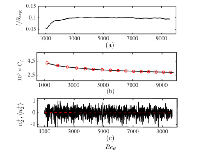
Figure 10: (a) Mean slip lengths $l$ normalised by $\theta_{\text{avg}}$, the average momentum thickness, (b) the friction coefficient from the LES with slip boundary condition (black —) and the empirical friction coefficient from White & Corfield (2006) (red $\circ$), and (c) the instantaneous (black solid line) and time-averaged (red dashed line) wall-normal velocities at the wall as a function of $\Rey_{\theta}$.

The mean streamwise velocity and the three rms velocity fluctuations at $\Rey_{\theta}\approx 6500$ ($\Rey_{\tau}\approx 1989.5$) are shown in figure 11 and compared with Sillero et al. (2013). As expected, the mean DNS and LES velocities match in the wake region, as the correct $C_{f}$ in the LES is imposed. The shape of the profile is also well predicted. The rms velocities are reasonably well reproduced at this Reynolds number, with no over-prediction of the streamwise rms velocity and under-prediction of the other two components close to the wall, consistent with the analysis in section 3.4.

\psfrag{X}[cc]{$x_{2}^{+}$}\psfrag{Y}[bc]{$\langle u_{1}^{+}\rangle$}\includegraphics[width=208.13574pt]{./figs/fig11a}

(a)

\psfrag{X}[cc]{$x_{2}^{+}$}\psfrag{Y}[bc]{$\langle u_{1}^{+}\rangle$}\psfrag{X}[cc]{$x_{2}/\delta$}\psfrag{Y}[bc]{$\langle u_{i}^{\prime 2+}\rangle^{1/2}$}\includegraphics[width=208.13574pt]{./figs/fig11b}

(b)

Figure 11: (a) Mean streamwise velocity profile and (b) rms streamwise ($\times$), spanwise ($\circ$), and wall-normal ($\triangledown$) fluctuation profiles at $\Rey_{\theta}\approx 6500$. Symbols are for LES. DNS from Sillero et al. (2013) (dashed line).

Overall, these results along with those from LES of channel flow in the previous sections show that the slip boundary condition successfully reproduces the one-point statistics of the flow as long as the slip lengths accurately reflect the correct mean wall stress.

Two more cases (not shown) were run to test the effect of the slip boundary condition on the net mass flow through the wall. In the first case, a slip boundary condition was imposed such that the net mass flow through the wall is positive (incoming flow through the wall) such that $\langle\bar{u}_{2}|_{w}\rangle_{w}\approx 0.01U_{\infty}$. In this case, the boundary layer thickness grew five times faster than the reference DNS. On the contrary, when the simulation was run with net negative mass flow through the walls ($\langle\bar{u}_{2}|_{w}\rangle_{w}\approx-0.01U_{\infty}$), the flow remained laminar. The results are consistent with observations in previous studies on blowing and suction of boundary layers (Simpson et al., 1969; Antonia et al., 1988; Chung & Sung, 2001; Yoshioka & Alfredsson, 2006) and highlight the relevance of imposing a correct zero net mass flow through the walls in order to faithfully predict the boundary layer growth.

4 Dynamic wall models for the slip boundary condition

It is pertinent to discuss first the expected role of wall models in LES. From section 3.3 and previous analysis in the literature (Lee et al., 2013), the most important requirement for a wall model is to supply accurate mean tangential stress at the wall. This requirement must be accompanied by an effective SGS model responsible for generating correct turbulence statistics in the outer region, where the wall model plays a secondary role. The first requirement is necessary for obtaining the correct bulk velocity, whereas the last point is crucial to predict the shape of the mean velocity profile and rms velocity fluctuations far from the wall (see sections 3.2 and 3.4).

The wall models reviewed in the introduction are capable of meeting the first requirement by assuming a specific state of the boundary layer and relying on empirical parameters consistent with such state. In this regard, most traditional wall models assume quasi-equilibrium turbulence in the vicinity of the wall and encode explicitly or implicitly information about the law of the wall, which cannot be derived from first principles but can only be extracted from DNS or wind tunnel experiments, such as the values of $\kappa$ and $B$. Despite the equilibrium-turbulence assumption, current wall-modelling approaches have been successful in predicting numerous flow configurations up to date, although their performance in some regimes such as transitional or separated flows as well as non-equilibrium turbulence is still open to debate.

The main purpose of a dynamic wall model is similar to that of traditional wall models, i.e., the estimation of accurate wall stress $\tau_{w}$. However, the objective is to achieve this goal without prior assumptions regarding the state of the boundary layer or embedded empirical parameters. Instead, dynamic wall models aim to use only the current (local) state of the LES velocity field and universal modelling assumptions valid across different flow scenarios. Note that the task outlined above is an outstanding challenge, since without any empirical coefficients there is no explicit reference to how the near wall flow should behave in different situations. Moreover, the instantaneous velocity field is intertwined with the effects of the LES grid resolution, Reynolds number, and SGS model choice as documented in previous sections. Additionally, numerical errors are amplified at the wall, and discretisation schemes are expected to play an important role as well. Dynamic models must encompass these factors in order to be of practical use, and whether this can be accomplished for arbitrary flow configurations remains to be demonstrated.

Despite the aforementioned difficulties, we provide below a dynamic slip wall model that shows the ability to adapt to different grid resolutions and Reynolds numbers as well as flow configurations, provided an SGS model. For a slip boundary condition of the form (1), the problem of estimating $\tau_{w}$ can be reformulated as finding the value of slip parameters that provides the correct mean wall stress. The relationship between $l$ and $\tau_{w}$ was shown in sections 3.2 and 3.6 for channels and boundary layers. Moreover, for the slip boundary condition to be used as a predictive tool in wall-modelled LES, the computed $l_{i}$ and $v_{i}$ should comply with the observations discussed in the previous sections.

4.1 Previous dynamic models

Bose & Moin (2014) introduced a dynamic wall model based on the slip boundary condition free of any a priori parameters. The slip length, assumed to be equal for the three spatial directions, is computed via a modified form of the Germano’s identity (Germano et al., 1991),

$$l^{2}\left(\Delta_{R}^{2}\frac{\partial\hat{\bar{u}}_{i}}{\partial n}\frac{\partial\hat{\bar{u}}_{j}}{\partial n}-\frac{\partial\bar{u}_{i}}{\partial n}\frac{\partial\bar{u}_{j}}{\partial n}\right)+T_{ij}^{\text{SGS}}-\widehat{\tau_{ij}}^{\text{SGS}}=\widehat{\bar{u}_{i}\bar{u}}_{j}-\bar{u}_{i}\bar{u}_{j},$$ (20)

where $l$ is the slip length, $(\hat{\cdot})$ is the test filter, $\Delta_{R}$ is the filter size ratio between the test and grid filters, $\tau_{ij}^{\text{SGS}}$ and $T_{ij}^{\text{SGS}}$ represent the grid and test filter SGS tensors, respectively. Equation (20) is then solved for $l$ by using least-squares.

In Bose & Moin (2014), the model was tested for a series of LES of turbulent channel flow and NACA 4412 airfoil. However, our attempts to reproduce the channel flow results did not perform as expected with our current implementation, which uses a different SGS model and numerical discretisation. The discrepancies motivated a deeper study of the slip boundary condition and investigation of alternative dynamic wall models as the one presented in the next section.

4.2 Wall-stress invariant dynamic wall model

We present a dynamic wall model formulated for the slip boundary condition based on the invariance of wall stress under test filtering. We will refer to this new model as wall-stress invariant model or WSIM. We will assume a single slip length $l_{1}=l_{2}=l_{3}=l$ and neglect any potential contribution from the terms $v_{i}$. The goal is to define a dynamic procedure to obtain $l$ at each time step such that the mean wall stress obtained from (14) is an accurate representation of the stress resulting from solving the Navier-Stokes equations with DNS resolution.

Let us consider the wall stress operator $\mathcal{T}_{ij}$ given by

$$\mathcal{T}_{ij}(\boldsymbol{u})=-R_{ij}(\boldsymbol{u})|_{w}-\tau^{\text{SGS}}_{ij}(\boldsymbol{u})|_{w}+2\nu S_{ij}(\boldsymbol{u})|_{w}-p(\boldsymbol{u})|_{w}\delta_{ij},$$ (21)

where terms $R_{ij}$, $\tau_{ij}^{\text{SGS}}$, $S_{ij}$ and $p\delta_{ij}$ are the Reynolds stress, subgrid stress, strain-rate, and pressure tensors, respectively, computed from the specified velocity field $\boldsymbol{u}$. In our formulation of $\mathcal{T}_{ij}$, the wall is assumed to be smooth, but the wall stress can be extended to encode information about the type of wall (smooth, rough, hydrophobic, etc.) by adding the appropriate drag terms into right-hand side of (21).

The modelling choice for the dynamic wall model is

$$\mathcal{T}_{ij}(\boldsymbol{\bar{u}})-\mathcal{T}_{ij}(\boldsymbol{\hat{\bar{u}}}) =0,$$ (22)

$$\mathcal{T}_{ij}(\boldsymbol{\hat{\hat{\bar{u}}}})-\widehat{\mathcal{T}_{ij}}(\boldsymbol{\hat{\bar{u}}}) =0,$$ (23)

where the different wall stresses, $\mathcal{T}_{ij}$, are obtained by either computing the stress of the filtered velocity field or by filtering the total stress. Condition (22) enforces the invariance of wall stress under test filtering and allows the wall model to predict the same wall stress regardless of the grid resolution (or filter). A similar approach was also adopted by Anderson & Meneveau (2011) for rough walls. Condition (23) is analogous to the Germano’s identity for the total stress of the filtered velocity and can be interpreted as a consistency condition between the wall stress and filter operator. The proposed model is given by combining (22) and (23) such that

$$\mathcal{F}_{ij}=\mathcal{T}_{ij}(\boldsymbol{\bar{u}})-\mathcal{T}_{ij}(\boldsymbol{\hat{\bar{u}}})+\mathcal{T}_{ij}(\boldsymbol{\hat{\hat{\bar{u}}}})-\widehat{\mathcal{T}}_{ij}(\boldsymbol{\hat{\bar{u}}})=0.$$ (24)

The rationale for this particular combination of (22) and (23) is given by considering $\mathcal{F}_{12}$, the dominant shear stress component in a boundary layer. This term can be simplified by test filtering only in the wall-normal direction with a box filter with filter size $\hat{\Delta}+x_{2}$ at $x_{2}<\hat{\Delta}$. Assuming that the subgrid stress tensor is given by an eddy viscosity, i.e., $(\tau_{ij}^{\text{SGS}}-1/3\delta_{ij}\tau_{kk}^{\text{SGS}})(\boldsymbol{\bar{u}})=-2\nu_{t}S_{ij}(\boldsymbol{\bar{u}})$ and that $\nu_{t}$ is constant in the near-wall region, the first order approximation of $\mathcal{F}_{12}$ can be shown to be

$$\mathcal{F}_{12}=\frac{\hat{\Delta}}{2}\left(\frac{\partial\bar{u}_{1}\bar{u}_{2}}{\partial x_{2}}-\frac{\partial}{\partial x_{2}}\left[(\nu+\nu_{t})|_{w}\frac{\partial\bar{u}_{1}}{\partial x_{2}}\right]\right)+\mathcal{O}(\hat{\Delta}^{2}).$$ (25)

Hence, $\mathcal{F}_{12}=0$ implicitly enforces the well-established constant stress layer across the wall-normal direction. Note that (22) and (23) may be combined differently to produce alternative versions of (24), but not all these groupings lead to a first order approximation consistent with the form reported in (25). For example, enforcing only (22) would not be consistant with (25). Nevertheless, wall models using different variants of (24) may be constructed based on similar principles; a broader family of dynamic models postulated on stress-invariant principles was investigated in Lozano-Durán et al. (2017).

Next we introduce an explicit dependence on the slip length condition in (24). We will assume that the slip boundary condition also applies for the test-filtered velocity field,

$$\hat{\bar{u}}_{i}=\hat{l}\frac{\partial\hat{\bar{u}}_{i}}{\partial n},$$ (26)

where $\hat{l}$ is the slip length at the test filter level. We will further suppose that a linear functional dependence of the slip length with the filter size of the form $\hat{l}=\Delta_{R}l$ holds. This assumption will be shown to be reasonably well satisfied in figure 14(c), which contains a posteriori values for the optimal slip length (15) as a function of grid resolution. Introducing the slip boundary condition at grid- and test-filter levels for the Reynolds stress terms in $\mathcal{T}_{ij}(\boldsymbol{\bar{u}})$ and $\mathcal{T}_{ij}(\boldsymbol{\hat{\bar{u}}})$, such that

$$\bar{u}_{i}\bar{u}_{j}=l^{2}\frac{\partial\bar{u}_{i}}{\partial n}\frac{\partial\bar{u}_{j}}{\partial n},\quad\hat{\bar{u}}_{i}\hat{\bar{u}}_{j}=l^{2}\Delta_{R}^{2}\frac{\partial\hat{\bar{u}}_{i}}{\partial n}\frac{\partial\hat{\bar{u}}_{j}}{\partial n},$$ (27)

the wall-stress invariant model becomes

$$l^{2}\left(\frac{\partial\bar{u}_{i}}{\partial n}\frac{\partial\bar{u}_{j}}{\partial n}-\Delta_{R}^{2}\frac{\partial\hat{\bar{u}}_{i}}{\partial n}\frac{\partial\hat{\bar{u}}_{j}}{\partial n}\right)=\bar{u}_{i}\bar{u}_{j}-\hat{\bar{u}}_{i}\hat{\bar{u}}_{j}+\mathcal{T}_{ij}(\boldsymbol{\bar{u}})-\mathcal{T}_{ij}(\boldsymbol{\hat{\bar{u}}})+\mathcal{T}_{ij}(\boldsymbol{\hat{\hat{\bar{u}}}})-\widehat{\mathcal{T}}_{ij}(\boldsymbol{\hat{\bar{u}}}),$$ (28)

which can be rewritten as

$$l^{2}\mathcal{M}_{ij}=\mathcal{L}_{ij}+\mathcal{F}_{ij},$$ (29)

with

$$\mathcal{M}_{ij}=\frac{\partial\bar{u}_{i}}{\partial n}\frac{\partial\bar{u}_{j}}{\partial n}-\Delta_{R}^{2}\frac{\partial\hat{\bar{u}}_{i}}{\partial n}\frac{\partial\hat{\bar{u}}_{j}}{\partial n},\quad\mathcal{L}_{ij}=\bar{u}_{i}\bar{u}_{j}-\hat{\bar{u}}_{i}\hat{\bar{u}}_{j},$$ (30)

The system (29) is over-determined and $l$ is computed via least-squares as

$$l^{2}=\frac{(\mathcal{L}_{ij}+\mathcal{F}_{ij})\mathcal{M}_{ij}}{\mathcal{M}_{ij}\mathcal{M}_{ij}}=\frac{\mathcal{L}+\mathcal{F}}{\mathcal{M}},$$ (31)

where repeated indices imply summation and the compact notation $\mathcal{L}=\mathcal{L}_{ij}\mathcal{M}_{ij}$, $\mathcal{F}=\mathcal{F}_{ij}\mathcal{M}_{ij}$, and $\mathcal{M}=\mathcal{M}_{ij}\mathcal{M}_{ij}$ is used. For incompressible flows, the isotropic part of $\tau_{ij}^{\text{SGS}}$ is usually not defined by the SGS models and, since the system is already over-determined, we exclude the $i=j$ components of (31).

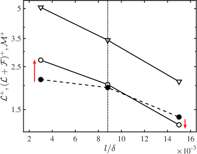
Figure 13:

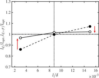
(a)

Figure 13: (a) $\mathcal{L}$ ($\bullet$), $\mathcal{L}+\mathcal{F}$ ($\circ$), and $\mathcal{M}$ ($\triangledown$) computed from LES of channel flow using the slip boundary condition with fixed $l$ equal to $l=0.35l_{\text{opt}}=0.003\delta$, $l=l_{\text{opt}}=0.009\delta$, and $l=1.70l_{\text{opt}}=0.015\delta$. (b) The slip lengths $l_{\mathcal{L}}$ ($\bullet$), $l_{\mathcal{L}+\mathcal{F}}$ ($\circ$) normalised by the optimal slip length. $\Delta_{R}$ was assigned to be $1.6$ (see section 5.1). The vertical dotted lines are $l=l_{\text{opt}}$. Red arrows highlight the improvement achieved by including the control term $\mathcal{F}_{ij}$. See text for more details.

Note that the first part of the right-hand-side of (28), $\bar{u}_{i}\bar{u}_{j}-\hat{\bar{u}}_{i}\hat{\bar{u}}_{j}$ ($\mathcal{L}_{ij}$), is the result of applying the boundary condition at the grid and test filter levels. The remaining terms, $\mathcal{T}_{ij}(\boldsymbol{\bar{u}})-\mathcal{T}_{ij}(\boldsymbol{\hat{\bar{u}}})+\mathcal{T}_{ij}(\boldsymbol{\hat{\hat{\bar{u}}}})-\widehat{\mathcal{T}}_{ij}(\boldsymbol{\hat{\bar{u}}})$ ($\mathcal{F}_{ij}$), then act as an effective control such that the slip length increases if the current wall stress is under-predicted, and decreases if the wall stress is over-predicted. This self-regulating mechanism can be examined by analysing the terms $\mathcal{M}$, $\mathcal{L}$, and $\mathcal{F}$ for three test cases of a channel flow at $Re_{\tau}\approx 4200$ with DSM and grid $\Delta_{1}=\Delta_{2}=\Delta_{3}=0.05\delta$. The first case is computed by imposing the optimal slip length, $l=l_{\text{opt}}=0.009\delta$. The second and third cases are analogous to the first case but with $l=1.70l_{\text{opt}}$ and $l=0.35l_{\text{opt}}$, respectively. The terms $\mathcal{M}$, $\mathcal{L}$, and $\mathcal{F}$ were evaluated after the cases were run with their corresponding slip lengths fixed in time until the statistically steady state was reached. Note that $\mathcal{L}$ can be interpreted as the model prior to applying the control mechanism, and this allows us to define two slip lengths, namely, $l_{\mathcal{L}}=\mathcal{L}/\mathcal{M}$ and $l_{\mathcal{L}+\mathcal{F}}=(\mathcal{L}+\mathcal{F})/\mathcal{M}$.

The terms $\mathcal{M}$, $\mathcal{L}$, and $\mathcal{L}+\mathcal{F}$ evaluated from the three test cases are plotted in figure 13(a), and the corresponding slip lengths $l_{\mathcal{L}}$ and $l_{\mathcal{L}+\mathcal{F}}$ are presented in figure 13(b). The results show that application of WSIM recovers the optimal slip length, and thus the correct wall stress, through the control mechanism $\mathcal{F}_{ij}$. The analysis provided here is performed a priori, that is, the wall model was used to predict $l$ at time $t+\Delta t$ for a given flow field at time $t$, but without an actual dynamic coupling between WSIM and LES. The remainder of the paper is devoted to test WSIM in LES under different test scenarios.

5 Performance of the wall-stress invariant model

5.1 Numerical experiments

To test the performance of WSIM, three flow configurations are considered: a statistically steady plane turbulent channel (2–D channel), a non-equilibrium three-dimensional transient channel (3–D channel), and a zero-pressure-gradient flat-plate turbulent boundary layer. The numerical methods of the simulations are the same as the ones given in sections 3.1 and 3.6. The 2–D channel flow and the turbulent boundary layer were discussed in section 3. The three-dimensional transient channel flow is a temporally developing turbulent boundary layer in a planar channel subjected to a sudden spanwise forcing as in Moin et al. (1990).

The size of the 2–D and 3–D channel domain is $8\pi\delta\times 2\delta\times 3\pi\delta$ in the streamwise, wall-normal and spanwise directions, respectively. For both 2–D and 3–D channel flows, periodic boundary conditions are applied in the streamwise and spanwise directions. For the top and bottom walls, we impose either the no-slip (NS), slip boundary condition for WSIM, or Neumann boundary condition for cases with the equilibrium wall model (EQWM). The formulation for the EQWM follows Kawai & Larsson (2013) with a matching location at the third grid cell for the streamwise velocity, although recent studies have shown that the first grid cell may be used for the EQWM when the velocities are filtered using a spatial or temporal filter (Yang et al., 2017) following the methodology first introduced for algebraic wall models (Bou-Zeid et al., 2004).

For the 2–D channel, the flow is driven by imposing a constant mean pressure gradient and the simulations are started from a random initial condition run for at least $100\delta/u_{\tau}$ after transients. In the case of the 3–D channel, the calculations were started from a 2–D fully developed plane channel flow driven by a streamwise mean pressure gradient. The subsequent calculations were performed with a transverse (spanwise) mean pressure gradient of $\partial P/\partial x_{3}=10\tau_{w0}/\delta$, where $\tau_{w0}$ is the mean wall shear stress of the unperturbed channel. The 3–D channel simulations were run for 10$u_{\tau 0}/\delta$ and averaged over seven realisations, where $u_{\tau 0}$ is the friction velocity of the 2–D initial condition.

For the boundary layer, the setup is identical to the one in section 3.6. The range of $\Rey_{\theta}$ is from 1000 to 10 000. The length, height and width of the simulated box are $L_{x}=1060\theta_{\text{avg}}$, $L_{y}=18\theta_{\text{avg}}$, and $L_{z}=35\theta_{\text{avg}}$ with the streamwise and spanwise resolutions of $\Delta_{1}/\delta=0.05$ ($\Delta_{1}^{+}=118$) and $\Delta_{3}/\delta=0.04$ ($\Delta_{3}^{+}=84.3$) at $\Rey_{\theta}\approx 6500$. The grid is slightly stretched in the wall-normal direction with minimum $\Delta_{2}/\delta=0.01$ ($\Delta_{2}^{+}=20.8$). The inlet, outlet, and top boundary conditions are as in section 3.6 with $x_{\text{ref}}/\theta_{0}=890$. For the wall, we impose the slip boundary condition for WSIM.

It is important to note the details of the filter operation, as dynamic wall models are particularly sensitive to this choice (see appendix A). Test filtering a variable $f$ in a given spatial direction at point $i$ is computed as $1/6f(i-1)+2/3f(i)+1/6f(i+1)$ (Simpson’s rule). The operation is repeated for all three directions away from the wall. This corresponds to a discrete fourth-order quadrature over a cell of size $2\Delta_{1}\times 2\Delta_{2}\times 2\Delta_{3}$ for a uniform grid. At the wall, the same filtering operation is used in the horizontal directions while the wall-normal filter is one-sided and given by $2/3f(1)+1/3f(2)$, with $f(1)$ and $f(2)$ denoting values at the first and second wall-normal grid points. This is an integration over a cell of size $2\Delta_{1}\times\Delta_{2}\times 2\Delta_{3}$. Also, the definition of the filter operation fixes the value of $\Delta_{R}$, which is the ratio between the grid and test filter sizes at the wall. In this case, the $\Delta_{R}$ based on the cell volume is given by $\sqrt[3]{2\times 1\times 2}\approx 1.6$.

The cases for the 2–D and 3–D channel are labelled following the convention ([Channel type]-[Wall model]-[Reynolds number]-[Grid]), where the grid labels G0, G1, and G2 given in table 2 correspond to $320\times 25\times 120$ ($\Delta_{1}=\Delta_{2}=\Delta_{3}=0.080\delta$), $512\times 40\times 192$ ($\Delta_{1}=\Delta_{2}=\Delta_{3}=0.050\delta$), and $1024\times 80\times 384$ ($\Delta_{1}=\Delta_{2}=\Delta_{3}=0.025\delta$), respectively. The wall model applied are labelled NS, EQWM, or WSIM. Additional cases with anisotropic grids, different values of $\Delta_{R}$, test-filtering operations, or SGS models were run to study the sensitivity of the model to these choices. They are discussed in Appendix A but not included in the table.

Grid label	$\Delta_{1}/\delta$	$\Delta_{2}/\delta$	$\Delta_{3}/\delta$
G0	$0.080$	$0.080$	$0.080$
G1	$0.050$	$0.050$	$0.050$
G2	$0.025$	$0.025$	$0.025$

Table 2: Grid resolutions in outer units. The first column contains the label used to name LES cases for the 2–D and 3–D channel flow simulations computed with different grids. The second, third, and fourth columns are the streamwise, wall-normal, and spanwise grid resolutions, respectively.

The 2–D channel results are compared with DNS data from Hoyas & Jiménez (2006) and Lozano-Durán & Jiménez (2014) for $\Rey_{\tau}\approx 2000$ and $4200$, Yamamoto & Tsuji (2018) for $\Rey_{\tau}\approx 8000$, and with the law-of-the wall for $\Rey_{\tau}>8000$. For the boundary layer, the resulting friction coefficient is compared to the empirical $C_{f}$ from White & Corfield (2006), and the mean velocity profiles are compared with the DNS data from Sillero et al. (2013) at $\Rey_{\theta}\approx 6500$ and the experimental data from Österlund (1999) at $\Rey_{\theta}\approx 8000$.

The performance of the WSIM in laminar flows has not been studied. However, in the limit of fine grids, the dynamic procedure of WSIM should produce zero slip lengths and revert to the no-slip boundary condition. Thus, for laminar cases with enough grid resolution to resolve the near-wall structures, we expect the dynamic wall model to naturally switch off.

5.2 Statistically steady two-dimensional channel flow

We assess the performance of WSIM compared to EQWM and NS. The results are discussed in terms of the error in the streamwise mean velocity profile across the logarithmic region. This choice was necessary in order to include higher Reynolds number cases where the corresponding DNS was not available and the law of the wall is used instead. Restricting the error to be evaluated only in the logarithmic layer is justified as wall models mainly impact the solution by vertically shifting the mean velocity profile and do not alter its shape for the range of grid resolutions tested as shown in section 3.3. In particular, the error is measured as the normalised $L_{2}$ error of the streamwise mean velocity between the second grid point and $0.2\delta$,

$$\mathcal{E}=\left[\frac{\int_{\Delta_{2}}^{0.2\delta}\left(\langle\bar{u}_{1}\rangle-\langle u_{1}^{\text{DNS}}\rangle\right)^{2}\mathrm{d}x_{2}}{\int_{\Delta_{2}}^{0.2\delta}\left(\langle u_{1}^{\text{DNS}}\rangle\right)^{2}\mathrm{d}x_{2}}\right]^{1/2}.$$ (32)

In the case where the corresponding DNS does not exist, $\langle u_{1}^{\text{DNS}}\rangle$ is replaced by the law of the wall,

$$\langle u_{1}^{\text{DNS}+}\rangle=\frac{1}{\kappa}\log x_{2}^{+}+B,$$ (33)

with $\kappa=0.392$ and $B=4.48$ (Luchini, 2017).

Figures 14(a) and (b) show $\mathcal{E}$ as a function of grid resolution and Reynolds number. At moderate Reynolds numbers ($\Rey_{\tau}<8000$) and all grid resolutions, the error for WSIM ($\mathcal{E}\approx$2–6%) is similar to that of the EQWM ($\mathcal{E}\approx$2–3%). With increasing Reynolds number, the performance degrades (up to $\mathcal{E}\approx$15% at $\Rey_{\tau}\approx$20 000), while the EQWM does not. The accurate results for EQWM are not surprising as its modelling assumptions are well satisfied for channel flow settings. The reason for the declining performance of WSIM at very high Reynolds number can be found in sections 2.1 and 2.2, where it was argued that the underlying assumptions for the slip condition are invalidated for large filter sizes. However, it is worth mentioning that the errors for an LES with no wall model ($\mathcal{E}\approx$100% for 2D-NS-4200-G1) are an order of magnitude larger than the errors of WSIM for all cases. The mean velocity profiles and streamwise rms velocity fluctuations for WSIM for various cases are shown in figure 15. Additional sensitivities to anisotropic grids, different values of $\Delta_{R}$, test-filtering operations, or SGS model are discussed in appendix A.

The slip lengths predicted by WSIM are shown in figure 14(c) and (d) as a function of grid resolution and Reynolds number and compared to the optimal slip lengths (15). It is remarkable that WSIM captures the overall behaviour of the optimal slip lengths, that is, a strong dependence on grid resolution and a weak variation with Reynolds number.

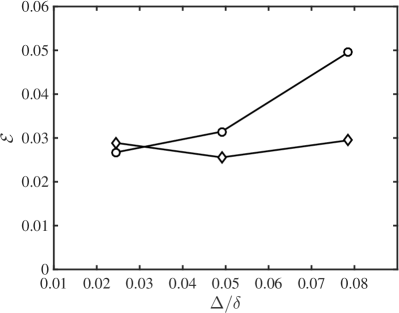
(a)

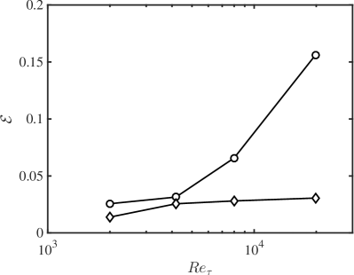
(b)

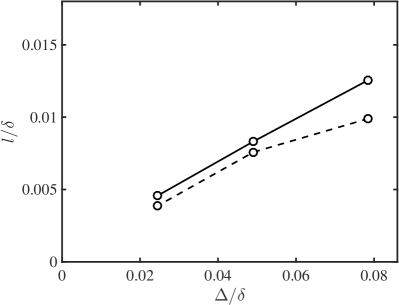
(c)

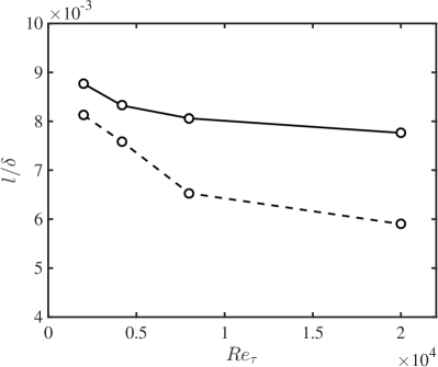
(d)

Figure 14: Error in the streamwise mean velocity profile, $\mathcal{E}$, as a function of (a) grid size (for $\Rey_{\tau}\approx 4200$) and (b) Reynolds number (for grid G1). WSIM ($\circ$) and EQWM ($\lozenge$). The predicted slip lengths $l/\delta$ for WSIM (solid lines) and optimal slip lengths (dashed lines) as a function of (c) grid resolution for $\Rey_{\tau}\approx 4200$ and (d) Reynolds number for grid G1.

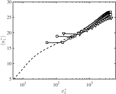
(a)

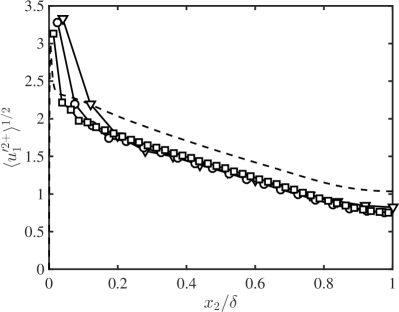
(b)

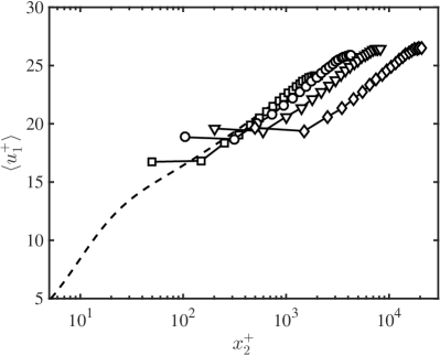
(c)

(d)

Figure 15: (a) Mean velocity profiles and (b) streamwise rms velocity fluctuations for WSIM at $\Rey_{\tau}\approx 4200$ for grid G0 ($\triangledown$), G1 ($\circ$), and G2 ($\square$). DNS for $\Rey_{\tau}\approx 4200$ (dashed line). (c) Mean velocity profiles and (d) streamwise rms velocity fluctuations for WSIM at $\Rey_{\tau}\approx 2000$ ($\square$), $4200$ ($\circ$), $8000$ ($\triangledown$), and 20 000 ($\lozenge$) for grid G1. DNS for $\Rey_{\tau}\approx 4200$ (dashed line).

5.3 Three-dimensional transient channel flow

The performance of WSIM in non-equilibrium scenarios is assessed in a three-dimensional transient channel flow (Moin et al., 1990). Note that in general wall models cannot be assumed to be effective at transferring information from the inner to the outer layer in non-equilibrium flows. Hence, the current flow set up, characterised by a spanwise boundary layer growing from the wall due to viscous effects, is expected to be problematic for wall-modelled LES. A plane channel flow was modified to incorporate a lateral (transverse) pressure gradient 10 times that of the streamwise pressure gradient. The details of the simulations were given in section 5.1.

The wall models explored are WSIM and EQWM. A case with the no-slip boundary condition is used for control, and the figure of merit is the evolution of the streamwise and spanwise wall stress as a function of time (figure 16). Note that the temporal increment of the wall stress magnitude involves an increase of the Reynolds number from $Re_{\tau}\approx 932$ at $t=0$ to $Re_{\tau}\approx 2600$ at $t=10\delta/u_{\tau 0}$. The results show that the performance of WSIM is similar to the EQWM despite its parameter-free nature. The streamwise and spanwise mean velocity profiles at various time instances are given in figure 17, which also shows that both WSIM and EQWM predict similar time evolutions. Although there is no reference DNS available for the full time span of our simulations, in the limited time range from $t=0$ to $1\delta/u_{\tau 0}$, Giometto et al. (2017) showed that the EQWM predicts the evolution of the wall stresses with less than 10% deviation in the spanwise wall stress prediction from DNS, and thus the results from WSIM are also expected to exhibit a similar error. Both the EQWM and WSIM entail a quantitative correction to the prediction provide by the no-slip boundary condition. Consequently, the computational simplicity and absence of a secondary mesh makes WSIM an appealing approach at the cost of a moderate attenuation of the predictive capabilities compared to more sophisticated wall models.

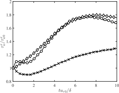
(a)

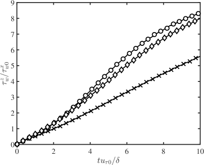
(b)

Figure 16: Wall stress in (a) streamwise and (b) spanwise directions as a function of time for WSIM ($\circ$), EQWM ($\lozenge$), and NS ($\times$).

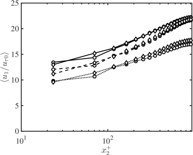
(a)

(b)

Figure 17: Mean (a) streamwise and (b) spanwise velocity profiles as a function of $x_{2}/\delta$ at $tu_{\tau 0}/\delta=0$ (solid lines), 4.5 (dashed lines), and 9 (dotted lines) for WSIM ($\circ$) and EQWM ($\lozenge$).

5.4 Zero-pressure-gradient flat-plate turbulent boundary layer

Finally, the performance of WSIM is assessed in a flat-plate turbulent boundary layer. The details of the numerical set-up were discussed in section 5.1. The friction coefficient is shown in figure 18 from $\Rey_{\theta}\approx 1000$ to 10 000. Note that the recycling scheme of Lund et al. (1998) imposes an artificial boundary condition at the inlet, requiring an initial development region for the flow to fully adapt to the slip boundary condition, which is the reason for the discrepancy in $C_{f}$ near the inlet. Consistent with previous test cases, the results show that WSIM predicts the friction coefficient well within $4\%$ error for $\Rey_{\theta}>6000$. The mean streamwise velocity profile at $\Rey_{\theta}\approx 6500$ and $8000$ and the rms velocity fluctuations at $\Rey_{\theta}\approx 6500$ are also well predicted as reported in figure 19.

\psfrag{X}[cc]{$\Rey_{\theta}$}\psfrag{Y}[bc][bc][1][180]{$10^{3}Cf$}\includegraphics[width=325.215pt]{./figs/fig17.eps}

Figure 18: Empirical friction coefficient from White & Corfield (2006) (red $\circ$) and the friction coefficient from WSIM (black —)

\psfrag{X}[cc]{$x_{2}/\delta$}\psfrag{Y}[bc]{$\langle u_{1}^{+}\rangle$}\includegraphics[width=208.13574pt]{./figs/fig18a.eps}

(a)

\psfrag{X}[cc]{$x_{2}/\delta$}\psfrag{Y}[bc]{$\langle u_{1}^{+}\rangle$}\psfrag{X}[cc]{$x_{2}/\delta$}\psfrag{Y}[bc]{$\langle u_{1}^{+}\rangle$}\includegraphics[width=208.13574pt]{./figs/fig18b.eps}

(b)

\psfrag{X}[cc]{$x_{2}/\delta$}\psfrag{Y}[bc]{$\langle u_{1}^{\prime 2+}\rangle^{1/2}$}\includegraphics[width=208.13574pt]{./figs/fig18c.eps}

(c)

\psfrag{X}[cc]{$x_{2}/\delta$}\psfrag{Y}[bc]{$\langle u_{1}^{\prime 2+}\rangle^{1/2}$}\psfrag{X}[cc]{$x_{2}/\delta$}\psfrag{Y}[bc]{$\langle u_{2,3}^{\prime 2+}\rangle^{1/2}$}\includegraphics[width=208.13574pt]{./figs/fig18d.eps}

(d)

Figure 19: Mean streamwise velocity profile for (a) $\Rey_{\theta}\approx 6500$ and (b) $\Rey_{\theta}\approx 8000$, and the rms (c) streamwise ($\times$), (d) spanwise ($\circ$), and wall-normal ($\triangledown$) fluctuation profiles at $\Rey_{\theta}\approx 6500$. WSIM (symbols) and DNS (Sillero et al., 2013) or experiment (Österlund, 1999) (dashed line).

6 Conclusions

Due to the scaling of grid resolution requirements in DNS and wall-resolved LES, wall-modelled LES stands as the most viable approach for most engineering applications. In most existing wall models, the Dirichlet no-slip boundary condition at the wall is replaced by a Neumann and no-transpiration conditions in the wall-parallel and wall-normal directions, respectively. In this study, we have investigated the efficacy of the Robin (slip) boundary condition, where the velocities at the wall are characterised by the slip lengths and slip velocities. One novel aspect of this boundary condition is the non-zero instantaneous wall-normal velocity at the wall, i.e., transpiration, that opens a new avenue to model near-wall turbulence in LES. We have also presented a new dynamic slip wall model, WSIM, that is free from a priori tunable RANS parameters, which most traditional wall models for LES rely on. The model is based on the invariance of the wall stress under test filtering and is effectively applied through the slip boundary condition.

We have provided theoretical support for the use of the slip condition in wall-modelled LES instead of the widely applied Neumann boundary condition with no-transpiration. A priori testing was performed to assess the validity of the slip condition in the context of filtered DNS data.

The slip boundary condition was implemented in LES of channel flow in order to gain a better insight into its capabilities and shortcomings. One of the key properties, made possible by transpiration, is that the correct wall stress can always be achieved by an appropriate combination of slip lengths. This property is crucial when the grid resolution in the near-wall region does not capture the buffer and logarithmic layer dynamics, which may result in an under- or over-prediction of the wall stress. We have derived the consistency conditions for coupling the wall stress with the slip boundary condition in channel flows and flat-plate boundary layers, and showed that such constraints are sufficient to guarantee the correct wall stress. Another advantage emanates from the non-zero Reynolds stress at the wall. This is not only consistent with the filtered velocity fields, but also alleviates the well-known problem of wall-stress under-estimation by commonly used SGS models. We have also assessed the sensitivities of one-point statistics to grid refinements, changes in $\Rey_{\tau}$, and different SGS models. The role of imposing zero mean mass flow through the wall by proper calculation of the slip parameters has also been shown to be a key component of the model.

Finally, we have tested the performance of a dynamic slip wall model, WSIM, in an LES of a plane turbulent channel flow at various Reynolds numbers and grid resolutions. The model was able to correctly capture the overall behaviour of the optimal slip length for a wide range of grid resolutions and Reynolds numbers. The results have been compared with those from the EQWM and the no-slip boundary condition. In all cases, WSIM performed substantially better than the no-slip, and the predictive error in the mean velocity profile was found to be below 10% for $\Rey_{\tau}<$ 10 000 and all grid resolutions investigated. The model was also tested for an LES of three-dimensional transient channel flow, where the performance was similar to that of the EQWM, and zero-pressure-gradient flat-plate turbulent boundary layer at $\Rey_{\theta}$ up to 10 000, where the error in the friction coefficient was less than 4%.

The present work has established the foundations and underlying principles for using the slip boundary condition for dynamic wall-modelled LES, free of a priori tunable parameters. Based on the principles laid out in this paper, new formulations of the wall-stress-invariant condition can be explored to account for the dependency on SGS models and numerical filtering operations documented in appendix A.

Appendix A Wall-stress invariant model: additional sensitivity analysis

Four additional cases were computed to analyse the sensitivity of the WSIM to $\Delta_{R}$, grid anisotropy, shape of the test filter, and choice of SGS model. The effect of $\Delta_{R}$ turned out to be negligible for the plausible range of values $\Delta_{R}=[1.4,1.8]$, and the measured difference in $\mathcal{E}$ was less than 1%. Regarding grid anisotropy, coarsening case 2D-WSIM-4200-G1 by a factor of two in the streamwise and spanwise directions had a negligible effect on $\mathcal{E}$. While coarsening in both the streamwise and spanwise directions simultaneously by a factor of two had a larger effect with $\mathcal{E}$ increasing to $\approx$8%. The error trend for anisotropic grids also follows the results shown in figure 14(a) when scaled with grid size based on cell volume, $\Delta=(\Delta_{1}\Delta_{2}\Delta_{3})^{1/3}$. This shows that the wall model is robust to mild grid anisotropies.

On the contrary, the test filter shape and SGS model highly impacted the prediction of the mean flow. Case 2D-WSIM-4200-G1 was repeated using test filter based on the trapezoidal rule, and the error increased from 2.5% to 32%. When 2D-WSIM-4200-G1 was run using the anisotropic minimum-dissipation (AMD) model (Rozema et al., 2015), the stress provided by the SGS model $\tau_{12}^{\text{SGS}}$ was larger than $u_{\tau}^{2}$, and the slip length prediction by WSIM was clipped to zero due to the excess of wall stress, reverting the boundary condition to no-slip. Although this is consistent with the fact that $\tau_{12}^{\text{SGS}}>u_{\tau}^{2}$ (see figure 8a), it also implies that the correct stress at the wall can never be obtained through the slip boundary condition with a single slip length in this case. It was shown in section 3 that the slip lengths in the wall-normal direction must be larger than the wall-parallel ones in order to drain the excess of stress supplied by the SGS model. This suggests that WSIM should be generalised to a formulation with a different slip length in each spatial direction to overcome this limitation. It also remains to study the near wall behaviour of various SGS models in the wall-modelled grid limits in more detail.

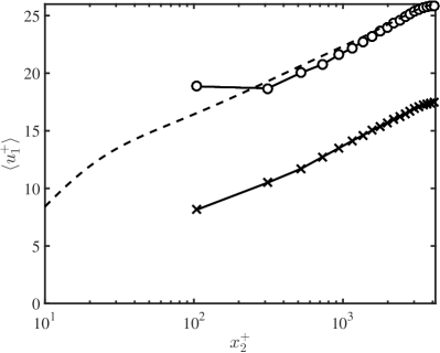
Figure 20: Mean streamwise velocity profile for WSIM for filter using Simpson’s rule ($\circ$) and trapezoidal rule ($\times$). DNS (dashed line). See section 5.1 for details regarding the test filter operators.

References

- Anderson & Meneveau (2011) Anderson, W. & Meneveau, C. 2011 Dynamic roughness model for large-eddy simulation of turbulent flow over multiscale, fractal-like rough surfaces. J. Fluid Mech. 679, 288–314.
- Antonia et al. (1988) Antonia, R. A., Fulachier, L., Krishnamoorthy, L. V., Benabid, T. & Anselmet, F. 1988 Influence of wall suction on the organized motion in a turbulent boundary layer. J. Fluid Mech. 190, 217–240.
- Bae & Lozano-Durán (2017) Bae, H. J. & Lozano-Durán, A. 2017 Towards exact subgrid-scale models for explicitly filtered large-eddy simulation of wall-bounded flows. Center for Turbulence Research - Annual Research Briefs pp. 207–214.
- Bae et al. (2018) Bae, H. J., Lozano-Durán, A., Bose, S. T. & Moin, P. 2018 Turbulence intensities in large-eddy simulation of wall-bounded flows. Phys. Rev. Fluids 3, 014610.
- Bae et al. (2016) Bae, H. J., Lozano-Durán, A. & Moin, P. 2016 Investigation of the slip boundary condition in wall-modeled LES. Center for Turbulence Research - Annual Research Briefs pp. 75–86.
- Balaras et al. (1996) Balaras, E., Benocci, C. & Piomelli, U. 1996 Two-layer approximate boundary conditions for large-eddy simulations. AIAA J. 34 (6), 1111–1119.
- Bose (2012) Bose, S. T. 2012 Explicitly filtered large-eddy simulation: with application to grid adaptation and wall modeling. PhD thesis, Stanford University.
- Bose & Moin (2014) Bose, S. T. & Moin, P. 2014 A dynamic slip boundary condition for wall-modeled large-eddy simulation. Phys. Fluids 26 (1), 015104.
- Bose & Park (2018) Bose, S. T. & Park, G. I. 2018 Wall-modeled les for complex turbulent flows. Ann. Rev. Fluid Mech. 50 (1), 535–561.
- Bou-Zeid et al. (2004) Bou-Zeid, E., Meneveau, C. & Parlange, M. B. 2004 Large-eddy simulation of neutral atmospheric boundary layer flow over heterogeneous surfaces: Blending height and effective surface roughness. Water Resour. Res. 40 (2).
- Cabot & Moin (2000) Cabot, W. H. & Moin, P. 2000 Approximate wall boundary conditions in the large-eddy simulation of high Reynolds number flow. Flow Turbul. Combust. 63, 269–291.
- Chapman (1979) Chapman, D. R. 1979 Computational aerodynamics development and outlook. AIAA J. 17 (12), 1293–1313.
- Choi & Moin (2012) Choi, H. & Moin, P. 2012 Grid-point requirements for large eddy simulation: Chapman’s estimates revisited. Phys. Fluids 24 (1), 011702.
- Chung & Pullin (2009) Chung, D. & Pullin, D. I. 2009 Large-eddy simulation and wall modelling of turbulent channel flow. J. Fluid Mech. 631, 281–309.
- Chung & Sung (2001) Chung, Y. M. & Sung, H. J. 2001 Initial relaxation of spatially evolving turbulent channel flow with blowing and suction. AIAA J. 39 (11), 2091–2099.
- Deardorff (1970) Deardorff, J. 1970 A numerical study of three-dimensional turbulent channel flow at large Reynolds numbers. J. Fluid Mech. 41 (1970), 453–480.
- Del Álamo et al. (2004) Del Álamo, J. C., Jiménez, J., Zandonade, P. & Moser, R. D. 2004 Scaling of the energy spectra of turbulent channels. J. Fluid Mech. 500, 135–144.
- Del Álamo et al. (2006) Del Álamo, J. C., Jiménez, J., Zandonade, P. & Moser, Robert D. 2006 Self-similar vortex clusters in the turbulent logarithmic region. J. Fluid Mech. 561, 329–358.
- Dong et al. (2017) Dong, S., Lozano-Durán, A., Sekimoto, A. & Jiménez, J. 2017 Coherent structures in homogeneous shear turbulence compared with those in channels. J. Fluid Mech. 816, 167–208.
- Flores & Jiménez (2006) Flores, O. & Jiménez, J. 2006 Effect of wall-boundary disturbances on turbulent channel flows. J. Fluid Mech. 566, 357–376.
- Germano et al. (1991) Germano, M., Piomelli, U., Moin, P. & Cabot, W. H. 1991 A dynamic subgrid-scale eddy viscosity model. Phys. Fluids A 3 (7), 1760.
- Ghosal & Moin (1995) Ghosal, S. & Moin, P. 1995 The basic equations for the large eddy simulation of turbulent flows in complex geometry. Journal of Computational Physics 118 (1), 24 – 37.
- Giometto et al. (2017) Giometto, B. M. G., Lozano-Durán, A., P., G. I. & Moin, P. 2017 Three-dimensional transient channel flow at moderate Reynolds numbers: analysis and wall modeling. Center for Turbulence Research - Annual Research Briefs pp. 193–205.
- Hoyas & Jiménez (2006) Hoyas, S. & Jiménez, J. 2006 Scaling of the velocity fluctuations in turbulent channels up to =2003. Phys. Fluids 18 (1), 011702.
- Jiménez (2013) Jiménez, J. 2013 Near-wall turbulence. Phys. Fluids 25 (10), 101302.
- Jiménez et al. (2010) Jiménez, J., Hoyas, S., Simens, M. P. & Mizuno, Y. 2010 Turbulent boundary layers and channels at moderate reynolds numbers. J. Fluid Mech. 657, 335–360.
- Jiménez & Moser (2000) Jiménez, J. & Moser, R. D. 2000 Large-eddy simulations: Where are we and what can we expect? AIAA J. 38 (4), 605–612.
- Kawai & Larsson (2013) Kawai, S. & Larsson, J. 2013 Dynamic non-equilibrium wall-modeling for large eddy simulation at high reynolds numbers. Phys. Fluids 25 (1), 015105.
- Kim & Moin (1985) Kim, J. & Moin, P. 1985 Application of a fractional-step method to incompressible Navier-Stokes equations. J. Comp. Phys. 59, 308–323.
- Larsson et al. (2016) Larsson, J., Kawai, S., Bodart, J. & Bermejo-Moreno, I. 2016 Large eddy simulation with modeled wall-stress: recent progress and future directions. Mech. Eng. Rev. 3 (1), 1–23.
- Lee et al. (2013) Lee, J., Cho, M. & Choi, H. 2013 Large eddy simulations of turbulent channel and boundary layer flows at high reynolds number with mean wall shear stress boundary condition. Physics of Fluids 25 (11), 110808.
- Leonard (1975) Leonard, A. 1975 Energy cascade in large-eddy simulations of turbulent fluid flows. Adv. Geophys. 18, 237–248.
- Lilly (1992) Lilly, D. K. 1992 A proposed modification of the Germano subgrid-scale closure method. Phys. Fluids A 4 (3), 633–635.
- Lozano-Durán et al. (2017) Lozano-Durán, A., Bae, H.J., Bose, S.T. & Moin, P. 2017 Dynamic wall models for the slip boundary condition. Center for Turbulence Research - Annual Research Briefs pp. 229–242.
- Lozano-Durán & Bae (2016) Lozano-Durán, A. & Bae, H. J. 2016 Turbulent channel with slip boundaries as a benchmark for subgrid-scale models in LES. Center for Turbulence Research - Annual Research Briefs pp. 97–103.
- Lozano-Durán et al. (2018) Lozano-Durán, A., Hack, M. J. P. & Moin, P. 2018 Modeling boundary-layer transition in direct and large-eddy simulations using parabolized stability equations. Phys. Rev. Fluids 3, 023901.
- Lozano-Durán & Jiménez (2014) Lozano-Durán, A. & Jiménez, J. 2014 Effect of the computational domain on direct simulations of turbulent channels up to = 4200. Phys. Fluids 26 (1), 011702.
- Lozano-Durán & Jiménez (2014) Lozano-Durán, A. & Jiménez, J. 2014 Time-resolved evolution of coherent structures in turbulent channels: characterization of eddies and cascades. J. Fluid Mech. 759, 432–471.
- Luchini (2017) Luchini, Paolo 2017 Universality of the turbulent velocity profile. Phys. Rev. Lett. 118, 224501.
- Lund (2003) Lund, T. S. 2003 The use of explicit filters in large eddy simulation. Comput. Math. App. 46 (4), 603–616.
- Lund & Kaltenbach (1995) Lund, T. S. & Kaltenbach, H. J. 1995 Experiments with explicit filtering for les using a finite-difference method. Center for Turbulence Research - Annual Research Briefs pp. 91–105.
- Lund et al. (1998) Lund, T. S., Wu, X. & Squires, K. D. 1998 Generation of turbulent inflow data for spatially-developing boundary layer simulations. J. Comp. Phys. 140 (2), 233–258.
- Marsden et al. (2002) Marsden, A. L., Vasilyev, O. V. & Moin, P. 2002 Construction of commutative filters for les on unstructured meshes. J. Comp. Phys. 175 (2), 584–603.
- Millikan (1938) Millikan, C. M. 1938 A critical discussion of turbulent flows in channels and circular tubes. In Proceedings of the Fifth International Congress for Applied Mathematics, Harvard and MIT.
- Mizuno & Jiménez (2013) Mizuno, Y. & Jiménez, J. 2013 Wall turbulence without walls. J. Fluid Mech. 723, 429–455.
- Moin et al. (1990) Moin, P., Shih, T.‐H., Driver, D. & Mansour, N. N. 1990 Direct numerical simulation of a three‐dimensional turbulent boundary layer. Physics of Fluids A: Fluid Dynamics 2 (10), 1846–1853.
- Nikitin (2007) Nikitin, N. 2007 Spatial periodicity of spatially evolving turbulent flow caused by inflow boundary condition. Phys. Fluids 19 (9), 091703.
- Orlandi (2000) Orlandi, P. 2000 Fluid Flow Phenomena: A Numerical Toolkit. Fluid Flow Phenomena: A Numerical Toolkit 1. Springer.
- Österlund (1999) Österlund, Jens M 1999 Experimental studies of zero pressure-gradient turbulent boundary layer flow. PhD thesis, Mekanik.
- Park & Moin (2014) Park, G. I. & Moin, P. 2014 An improved dynamic non-equilibrium wall-model for large eddy simulation. Phys. Fluids 26 (1), 015108.
- Pauley et al. (1990) Pauley, L. L., Moin, P. & Reynolds, W. C. 1990 The structure of two-dimensional separation. J. Fluid Mech. 220, 397–411.
- Piomelli & Balaras (2002) Piomelli, U. & Balaras, E. 2002 Wall-layer models for large-eddy simulations. Annu. Rev. Fluid Mech. 34, 349–374.
- Piomelli et al. (1989) Piomelli, U., Ferziger, J., Moin, P. & Kim, J. 1989 New approximate boundary conditions for large eddy simulations of wall-bounded flows. Phys. Fluids A 1 (6), 1061–1068.
- Prandtl (1925) Prandtl, L. 1925 Bericht über Untersuchungen zur ausgebildeten Turbulenz. Zeitschrift fuer Angewandte Mathematik und Mechanik 5, 136–139.
- Rozema et al. (2015) Rozema, W., Bae, H. J., Moin, P. & Verstappen, R. 2015 Minimum-dissipation models for large-eddy simulation. Phys. Fluids 27 (8), 085107.
- Schlatter & Örlü (2010) Schlatter, P. & Örlü, R. 2010 Assessment of direct numerical simulation data of turbulent boundary layers. J. Fluid Mech. 659, 116.
- Schumann (1975) Schumann, U. 1975 Subgrid scale model for finite difference simulations of turbulent flows in plane channels and annuli. J. Comp. Phys. 18, 376–404.
- Sillero et al. (2013) Sillero, J. A., Jiménez, J. & Moser, R. D. 2013 One-point statistics for turbulent wall-bounded flows at reynolds numbers up to . Phys. Fluids 25 (10), 105102.
- Silvis et al. (2016) Silvis, M. H., Trias, F. X., , Abkar, M, Bae, H. J., Lozano-Durán, A. & Verstappen, R. 2016 Exploring nonlinear subgrid-scale models and new characteristic length scales for large-eddy simulation. Center for Turbulence Research - Proceedings of the Summer Program pp. 265–274.
- Simens et al. (2009) Simens, M. P., Jiménez, J., Hoyas, S. & Mizuno, Y. 2009 A high-resolution code for turbulent boundary layers. J. Comp. Phys. 228 (11), 4218–4231.
- Simpson et al. (1969) Simpson, R. L., Moffat, R. J. & Kays, W. M. 1969 The turbulent boundary layer on a porous plate: experimental skin friction with variable injection and suction. Int. J. Heat Mass Transfer 12 (7), 771–789.
- Smagorinsky (1963) Smagorinsky, J. 1963 General circulation experiments with the primitive equations. Mon. Weather Rev. 91 (3), 99–164.
- Spalart (2009) Spalart, P. R. 2009 Detached-eddy simulation. Annu. Rev. Fluid Mech. 41, 181–202.
- Spalart et al. (1997) Spalart, P. R., Jou, W. H., Strelets, M., Allmaras, S. R. & others 1997 Comments on the feasibility of LES for wings, and on a hybrid RANS/LES approach. Advances in DNS/LES 1, 4–8.
- Stokes et al. (1901) Stokes, G. G. & others 1901 Mathematical and physical papers.
- Townsend (1980) Townsend, A. A. 1980 The structure of turbulent shear flow. Cambridge Univ Press.
- Wang & Moin (2002) Wang, M. & Moin, P. 2002 Dynamic wall modeling for large-eddy simulation of complex turbulent flows. Phys. Fluids 14 (7), 2043–2051.
- White & Corfield (2006) White, F. M. & Corfield, I. 2006 Viscous fluid flow, , vol. 3. McGraw-Hill New York.
- Wray (1990) Wray, A. A. 1990 Minimal-storage time advancement schemes for spectral methods. Tech. Rep.. NASA Ames Research Center.
- Yamamoto & Tsuji (2018) Yamamoto, Y. & Tsuji, Y. 2018 Numerical evidence of logarithmic regions in channel flow at . Phys. Rev. Fluids 3, 012602.
- Yang et al. (2017) Yang, X. I. A., Park, G. I. & Moin, P. 2017 Log-layer mismatch and modeling of the fluctuating wall stress in wall-modeled large-eddy simulations. Phys. Rev. Fluids 2, 104601.
- Yang et al. (2015) Yang, X. I. A., Sadique, J., Mittal, R. & Meneveau, C. 2015 Integral wall model for large eddy simulations of wall-bounded turbulent flows. Phys. Fluids 27 (2), 025112.
- Yoshioka & Alfredsson (2006) Yoshioka, S. & Alfredsson, P. H. 2006 Control of turbulent boundary layers by uniform wall suction and blowing, pp. 437–442. Dordrecht: Springer Netherlands.