Resolvent Trace Asymptotics on Stratified Spaces

Abstract.

Let $(M,g)$ be a compact smoothly stratified pseudomanifold with an iterated cone-edge metric satisfying a spectral Witt condition. Under these assumptions the Hodge-Laplacian $\Delta$ is essentially self-adjoint. We establish the asymptotic expansion for the resolvent trace of $\Delta$. Our method proceeds by induction on the depth and applies in principle to a larger class of second-order differential operators of regular-singular type, e.g., Dirac Laplacians. Our arguments are functional analytic, do not rely on microlocal techniques and are very explicit. The results of this paper provide a basis for studying index theory and spectral invariants in the setting of smoothly stratified spaces and in particular allow for the definition of zeta-determinants and analytic torsion in this general setup.

1. Introduction and statement of the main results

Stratified spaces with iterated cone-edge metrics provide a natural class of singular spaces which encompasses algebraic varieties, various moduli spaces as well as limits of families of smooth spaces under controlled degenerations. Analytic techniques in the singular setting date back to Kondratiev [Kon67] in the early 1960’s. In a seminal series of papers Cheeger [Che79, Che80, Che83] initiated the program of “extending the theory of the Laplace operator to certain Riemannian spaces with singularities”.

Subsequently, a flow of publications was inspired by Cheeger’s work. Geometric operators on spaces with isolated conical and cylindrical singularities became a central aspect of research by Brüning and Seeley [BrSe85, BrSe87, BrSe91], Lesch [Les97], Melrose [Mel93], Schulze [Sch91], and many more. Elliptic theory in the setting of non-isolated conical singularities, the so-called edge (wedge) singularities( cf. Figure 1), was developed by Mazzeo [Maz91], as well as Schulze [Sch89, Sch02] and his collaborators.

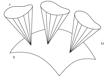
Figure 1. Simple Edge as a Cone bundle over $B$.

Elliptic theory and index theoretic problems in the general setting of stratified spaces have been studied by Albin-Leichtnam-Mazzeo-Piazza [ALMP12, ALMP13] and Akutagawa-Carron-Mazzeo [ACM14].

Let $(M,g)$ be a compact smoothly stratified pseudomanifold with an iterated cone-edge metric satisfying a spectral Witt condition. Under these assumptions the Hodge-Laplacian $\Delta$ is essentially self-adjoint. The present paper establishes the asymptotic expansion for the resolvent trace of $\Delta$. The argument applies in principle to a larger class of second-order differential operators of regular-singular type e.g., Dirac Laplacians. Our main result can be viewed as one of the ultimate goals of Cheeger’s spectral geometric program and reads as follows.

Theorem 1.1.

Let $(M,g)$ be a compact smoothly stratified pseudomanifold with an iterated cone-edge metric and depth $d$ satisfying the spectral Witt condition, cf. Section 2.2 and Definition 4.1 below. Denote by $\Delta$ the corresponding Hodge-Laplacian. Then $\Delta$ is essentially self-adjoint. Moreover, for $2m>\dim M$ the $m$-th power $(\Delta+z^{2})^{-m}$ of the resolvent is trace class and its trace admits the following asymptotic expansion as $z\to\infty$

$$\begin{split}\operatorname{tr}\,(\Delta+z^{2})^{-m}\sim z^{-2m}\cdot\Bigl{(}\sum_{j=0}^{\infty}a_{j}\cdot z^{-j+\dim M}+\sum_{\{Y\}}\sum_{j=0}^{\infty}\sum_{\ell=0}^{d(Y)}c^{Y}_{j\ell}\cdot z^{-j+\dim Y}\log^{\ell}z\Bigr{)},\end{split}$$

where the second summation is over all singular strata $\{Y\}$ and $d(Y)$ denotes the depth of the stratum $Y$.

A priori we cannot exclude any of the coefficients in the asymptotic expansion. In particular, the resolvent trace asymptotics may admit terms of the form $z^{-2m}\log(z)$, which cannot be excluded by an even-odd calculus argument as in [MaVe12], unless the stratification depth $d$ equals $1$.

A recent preprint by Albin and Gell-Redman [AlGR17] addresses the resolvent asymptotics on stratified spaces by completely different techniques than in the present paper. While [AlGR17] relies on an intricate microlocal blowup analysis, our paper is completely independent and follows rather a functional analytic approach motivated by Brüning and Seeley [BrSe91].

In particular, we use the well-known Singular Asymptotics Lemma (SAL) [BrSe87, p. 372], the Trace Lemma [BrSe91, Lemma 4.3], as well as the explicit construction of the Legendre operator in [BrSe87, Lemma 3.5] and [BrSe91, Theorem 4.1], and the proof of integrability in SAL in [BrSe91, Lemma 5.5].

Our paper is organized as follows. We first recall the fundamentals of smoothly stratified pseudomanifolds in §2, and the structure of the Hodge-Laplacian for iterated cone-edge metrics in §3. In §4 we recall the main results of our previous paper [HLV18] on the domains of the Gauss-Bonnet and Hodge-Laplace operators on a smoothly stratified pseudomanifold. In §5 we recall the notions of Hilbert scales and define weighted Sobolev spaces on abstract cones and edges, as in [HLV18]. In §6 we extend the results of [HLV18] to study the resolvent of the Bessel operator on a model cone. In §7 the results on the Bessel operator are used in order to study the resolvent of a Laplace operator on a model edge, extending [HLV18]. In §8, we apply the Singular Asymptotics Lemma with parameters (Appendix) to establish an asymptotic expansion for the trace of the resolvent on a model edge. We then conclude the paper with a proof of our main result by induction on the depth of the stratification in §9.

Acknowledgments

The authors thank the São Paulo Research Foundation, Brazil, the DFG Priority Programme ”Geometry at Infinity” and the Hausdorff Center for Mathematics in Bonn, Germany. The third author would like to thank the Federal University of São Carlos (UFSCar) for hospitality during the various phases of the project.

2. Smoothly stratified spaces and iterated cone-edge metrics

In this section we recall basic aspects of the definition of a compact smoothly stratified space of depth $d\in\mathbb{N}_{0}$, referring the reader for a complete discussion, e.g., to [ALMP12, ALMP13, Alb16].

2.1. Smoothly stratified spaces of depth zero and one

A compact smoothly stratified space of depth zero is by definition a smooth compact manifold. A compact smoothly stratified space $M$ of depth one consists by definition of a smooth open and dense stratum $M_{\operatorname*{reg}}$, a singular stratum $Y$, which is a closed compact manifold, and its tubular neighborhood $\mathscr{U}\subset M$. The tubular neighborhood $\mathscr{U}$ is the total space of a fibration $\phi:\mathscr{U}\to Y$ with fibres given by $[0,1)\times F/_{(0,\theta_{1})\sim(0,\theta_{2})}$, where $F$ is a smooth compact manifold. An incomplete edge metric $g$ on $M$ is by definition smooth away from the stratum $Y$, and is given in $\mathscr{U}\cap M_{\operatorname*{reg}}$ by

$$g|_{\mathscr{U}\cap M}=dx^{2}+\phi^{\ast}g_{Y}+x^{2}g_{F}+h=:g_{0}+h,$$ (2.1)

where $g_{Y}$ is a smooth Riemannian metric on the stratum $Y$, $g_{F}$ is a symmetric two tensor on the level set $\{x=1\}$, whose restriction to the links $F$ is a smooth family of Riemannian metrics. The higher order term $h$ satisfies $|h|_{g_{0}}=O(x)$, when $x\to 0$, where $|\cdot|_{g_{0}}$ denotes the norm on symmetric $2$-tensors of $T^{*}M_{\operatorname*{reg}}$ induced by the leading term $g_{0}$.

2.2. Smoothly stratified spaces of arbitrary depth d

We say that $M$ is a compact smoothly stratified space of depth $d\geq 2$ with strata $\{Y_{\alpha}\}_{\alpha\in A}$, where each stratum is identified with its interior, if $M$ is compact and the following, inductively defined, properties are satisfied:

1. If $Y_{\alpha}\cap\overline{Y}_{\beta}\neq\varnothing$ then $Y_{\alpha}\subset\overline{Y}_{\beta}$.

2. The depth of a stratum $Y$ is the largest $j\in\mathbb{N}_{0}$ such that there exists a chain of pairwise distinct strata $\{Y=Y_{j},\;Y_{j-1},\ldots,Y_{1},Y_{0}=M_{\operatorname*{reg}}\}$ with $Y_{i}\subset\overline{Y}_{i-1}$ for all $1\leq i\leq j$.

3. The stratum of maximal depth is smooth and compact. The maximal depth of any stratum of $M$ is called the depth of $M$.

4. Any point of $Y_{\alpha}$, a stratum of depth $j$, has a tubular neighborhood $\mathscr{U}_{\alpha}\subset M$, which is a total space of a fibration $\phi_{\alpha}:\mathscr{U}_{\alpha}\to\phi_{\alpha}(\mathscr{U}_{\alpha})\subseteq Y_{\alpha}$ with fibers given by cones $[0,1)\times F_{\alpha}/_{(0,\theta_{1})\sim(0,\theta_{2})}$, with link $F_{\alpha}$ being a compact smoothly stratified space of depth $j-1$.

5. Let $X_{j}$ be the union of all strata of dimension less or equal than $j$. The $M=X_{n}$ and $X_{n}\setminus X_{n-1}$ is an open smooth manifold dense in $M$.

6. If in addition $X_{n-1}=X_{n-2}$, i.e., there is no stratum of dimension $\dim M-1=n-1$ then we call $M$ a smoothly stratified pseudomanifold. In this case we have

   $$M=X_{n}\supset X_{n-1}=X_{n-2}\supseteq X_{n-3}\supseteq\cdots\supseteq X_{1}\supseteq X_{0}.$$

We call the union $X_{n-2}$ of all $Y_{\alpha}$, $\alpha\in A$, the singular part of $M$, and its complement in $M$, the regular part $M_{\operatorname*{reg}}$ of $M$. The precise definition of compact smoothly stratified spaces is more involved, [ALMP12, ALMP13] and [Alb16].

We define an iterated cone-edge metric $g$ on $M$ by asking $g$ to be a smooth Riemannian metric away from the singular strata, and requiring it to be in each tubular neighborhood $\mathscr{U}_{\alpha}$ of any point in $Y_{\alpha}$ of the form

$$g|_{\mathscr{U}_{\alpha}\cap M}=dx^{2}+\phi^{\ast}_{\alpha}g_{Y_{\alpha}}+x^{2}g_{F_{\alpha}}+h=:g_{0}+h,$$ (2.2)

where the restriction $g_{Y_{\alpha}}\restriction\phi_{\alpha}(\mathscr{U}_{\alpha})$ is a smooth Riemannian metric, $g_{F_{\alpha}}$ is a symmetric two tensor on the level set $\{x=1\}$, whose restriction to the links $F_{\alpha}$ (smoothly stratified spaces of depth at most $(j-1)$) is a smooth family of iterated cone-edge metrics. The higher order term $h$ satisfies as before $|h|_{g_{0}}=O(x)$, when $x\to 0$.

We also assume that $\phi_{\alpha}|_{\partial\mathscr{U}_{\alpha}}:(\partial\mathscr{U}_{\alpha},g_{F_{\alpha}}+\phi^{\ast}_{\alpha}g_{Y_{\alpha}})\to(\phi_{\alpha}(\mathscr{U}_{\alpha}),g_{Y_{\alpha}})$ is a Riemannian submersion and put the same condition in the lower depth. The existence of such iterated cone-edge metrics is discussed in [ALMP12, Proposition 3.1]. A compact smoothly stratified space of depth $2$ with an iterated cone-edge metric is illustrated in Figure 2.

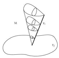
Figure 2. Tubular neighborhood $\mathscr{U}\subset M$, $M$ of depth $2$.

2.3. Resolution of singularities and edge vector fields

The singularities of $M$ can be resolved as follows. The resolution $\widetilde{M}$ is defined iteratively by replacing the cones in the fibrations $\phi_{\alpha}$ with finite cylinders $[0,1)\times F_{\alpha}$, and subsequently replacing the compact smoothly stratified space $F_{\alpha}$ of lower depth with its resolution $\widetilde{F}_{\alpha}$ as well. This defines a compact manifold with corners [ALMP12, Section 2]. The same procedure applies to any tubular neighborhood $\mathscr{U}_{\alpha}$, leading to its resolution $\widetilde{\mathscr{U}}_{\alpha}$.

The iterated edge vector fields $\mathcal{V}_{e,d}$ as well as the iterated incomplete edge vector fields $\mathcal{V}_{ie,d}$ on the compact smoothly stratified space $M$ are defined by an inductive procedure. In case $d=0$, both are simply the smooth vector fields. For $d\geq 1$, we denote by $\rho$ a smooth function on the resolution $\widetilde{M}$, nowhere vanishing in its open interior, and vanishing to first order at each boundary face. Then $\mathcal{V}_{e,d}=\rho\mathcal{V}_{ie,d}$ are by definition smooth vector fields in the open interior $M_{\operatorname*{reg}}$, and for any tubular neighborhood $\mathscr{U}_{\alpha}$ with radial function $x$ and local coordinates $\{s_{1},\ldots,s_{\dim Y_{\alpha}}\}$ in $\phi_{\alpha}(\mathscr{U}_{\alpha})\subseteq Y_{\alpha}$, we set

$$\begin{split}&\mathcal{V}_{e,d}\restriction\widetilde{\mathscr{U}}_{\alpha}=C^{\infty}(\widetilde{\mathscr{U}}_{\alpha})\textup{- span}\,\{\rho\partial_{x},\rho\partial_{s_{1}},...,\rho\partial_{s_{\dim Y_{\alpha}}},\mathcal{V}_{e,d-1}(F_{\alpha})\},\\ &\mathcal{V}_{ie,d}\restriction\widetilde{\mathscr{U}}_{\alpha}=C^{\infty}(\widetilde{\mathscr{U}}_{\alpha})\textup{- span}\,\{\partial_{x},\partial_{s_{1}},...,\partial_{s_{\dim Y_{\alpha}}},\rho^{-1}\mathcal{V}_{e,d-1}(F_{\alpha})\}.\end{split}$$ (2.3)

2.4. Sobolev spaces on compact smoothly stratified pseudomanifolds

Consider a compact smoothly stratified pseudomanifold $M$ of depth $d$ with an iterated cone-edge metric $g$. Consider the incomplete edge tangent bundle ${}^{ie}TM$ canonically defined by the condition that the incomplete edge vector fields $\mathcal{V}_{ie,d}$ form (locally) a spanning set of sections $\mathcal{V}_{ie,d}=C^{\infty}(M,{}^{ie}TM)$. We write ${}^{ie}T^{*}M$ for the dual of ${}^{ie}TM$, which we call the incomplete edge cotangent bundle. We define the edge Sobolev spaces with values in $\Lambda^{*}({}^{ie}T^{*}M)$ as follows.

Definition 2.1.

Let $M$ be a compact smoothly stratified pseudomanifold of depth $d\in\mathbb{N}_{0}$ with an iterated cone-edge metric $g$. We denote by $L^{2}_{*}(M)$ the $L^{2}$ completion of smooth compactly supported differential forms

$${}^{ie}\Omega_{0}^{*}(M_{\operatorname*{reg}}):=C^{\infty}_{0}(M_{\operatorname*{reg}},\Lambda^{*}({}^{ie}T^{*}M)).$$ (2.4)

Denote by $\rho$ a smooth function on the resolution $\widetilde{M}$, nowhere vanishing in its open interior, and vanishing to first order at each boundary face. Then, for any $s\in\mathbb{N}_{0}$ and $\delta\in\mathbb{R}$ we define the weighted edge Sobolev spaces by

$$\begin{split}&\mathscr{H}_{e}^{s}(M):=\{\mathrm{\omega}\in L^{2}_{*}(M)\mid V_{1}\circ\cdots\circ V_{s}\mathrm{\omega}\in L^{2}_{*}(M),\ \textup{for}\ V_{j}\in\mathcal{V}_{e,d}\},\\ &\mathscr{H}_{e}^{s,\delta}(M):=\{\mathrm{\omega}=\rho^{\delta}u\mid u\in\mathscr{H}_{e}^{s}(M)\},\end{split}$$ (2.5)

where $V_{1}\circ\cdots\circ V_{s}\mathrm{\omega}\in L^{2}_{*}(M)$ is understood in the distributional sense.

3. Hodge-Laplacian on a smoothly stratified pseudomanifold

Consider a compact smoothly stratified pseudomanifold $M$ with an iterated cone-edge metric $g$. Let $d$ denote the exterior derivative acting on compactly supported differential forms on $M_{\operatorname*{reg}}$, and $d^{t}$ be its formal adjoint with respect to the $L^{2}$-inner product induced by the Riemannian metric $g$. Then the Gauss-Bonnet operator of $(M,g)$ is defined by $D:=d+d^{t}$. The Hodge-Laplacian is defined as

$$\Delta=D^{t}D=d^{t}d+dd^{t}.$$

We now discuss the singular structure of the Gauss-Bonnet operator $D$ and the Hodge-Laplacian $\Delta$.

3.1. Rescaling transformation on isolated cones

Consider for the moment the special case of $(M_{\operatorname*{reg}},g_{0})$ being an open truncated cone $M_{\operatorname*{reg}}=(0,1)\times F$ over a compact smooth Riemannian manifold $(F,g_{F})$ of dimension $f=\dim F$ and $g_{0}=dx^{2}+x^{2}g_{F}$. In this setting, $D$ and $\Delta$, acting on smooth compactly supported differential forms, can be written in a concise form using a rescaling, already employed by Brüning-Seeley [BrSe88, Section 5]

$$\begin{split}S_{0}:C^{\infty}_{0}((0,1),\Omega^{k-1}(F)\times\Omega^{k}(F))\to\Omega^{k}((0,1)\times F),\\ (\mathrm{\omega}_{k-1},\mathrm{\omega}_{k})\mapsto x^{k-1-\frac{f}{2}}\mathrm{\omega}_{k-1}\wedge dx+x^{k-\frac{f}{2}}\mathrm{\omega}_{k}.\end{split}$$ (3.1)

This rescaling extends to a unitary transformation on the $L^{2}$-completions. The transformed operators take the form

$$\begin{split}&S_{0}^{-1}\circ D\circ S_{0}=\Gamma\left(\frac{d}{dx}+\frac{1}{x}Q\right),\\ &S_{0}^{-1}\circ\Delta\circ S_{0}=\left(-\frac{d^{2}}{dx^{2}}+\frac{1}{x^{2}}\bigl{(}A-\frac{1}{4}\bigr{)}\right),\end{split}$$ (3.2)

where $Q$ is a self-adjoint operator in $L^{2}(\Omega^{*}(F))$ and $A=Q(Q+1)+\frac{1}{4}=(Q+\frac{1}{2})^{2}$. We want to reinterpret the transformation $S_{0}$ using incomplete edge cotangent bundles. In fact, writing $X$ for the multiplication operator, multiplying by $x\in(0,1)$, we find

$$\begin{split}{}^{ie}\Omega^{k}((0,1)\times F)&\equiv C^{\infty}((0,1),X^{k-1}\Omega^{k-1}(F)\times X^{k}\Omega^{k}(F)),\\ L^{2}({}^{ie}\Omega^{k}((0,1)\times F),g_{0})&=L^{2}((0,1),x^{f}dx;\ X^{k-1}L^{2}(\Omega^{k-1}(F))\otimes X^{k}L^{2}(\Omega^{k}(F))).\end{split}$$

The rescaling $S_{0}$ now yields the following map

where $\omega=x^{k-1}dx\wedge\omega_{k-1}+x^{k}\omega_{k}$. The use of incomplete edge cotangent bundles not only simplifies the action of the Brüning-Seeley rescaling $S_{0}$, but is also a convenient way to discuss higher depth stratified spaces where the cross section $F$ is a stratified space itself.

3.2. Rescaling transformation on a tubular neighborhood $\mathscr{U}_{\alpha}$ of a stratum

We proceed in the notation of §2 and consider a tubular neighborhood $\mathscr{U}_{\alpha}$ of a point in a singular stratum $Y_{\alpha}$, where the edge metric is of the form

$$g|_{\mathscr{U}_{\alpha}}=dx^{2}+\phi^{\ast}_{\alpha}g_{Y_{\alpha}}+x^{2}g_{F_{\alpha}}+h=:g_{0}+h.$$ (3.3)

The operators $D$ and $\Delta$ restricted to $\mathscr{U}_{\alpha}$ act on compactly supported smooth differential forms ${}^{ie}\Omega_{0}^{*}(Y_{\alpha}\times C(F_{\alpha,\operatorname*{reg}}))=C^{\infty}_{0}(Y_{\alpha}\times C(F_{\alpha,\operatorname*{reg}}),{}^{ie}\Lambda^{*}T^{*}(Y_{\alpha}\times C(F_{\alpha,\operatorname*{reg}})))$, where $C(F_{\alpha,\operatorname*{reg}})=(0,1)\times F_{\alpha,\operatorname*{reg}}$ and we employ the notation introduced in (2.4). We write $f=\dim F_{\alpha}$, denote by $(s)$ the local variables on $Y_{\alpha}$, and by $x\in(0,1)$ the radial function on the cone $C(F_{\alpha})$. We rewrite $D$ and $\Delta$ using the rescaling from the previous section:

$$S:{}^{ie}\Omega_{0}^{*}(Y_{\alpha}\times C(F_{\alpha,\operatorname*{reg}}))\to{}^{ie}\Omega_{0}^{*}(Y_{\alpha}\times C(F_{\alpha,\operatorname*{reg}})),$$

$$\qquad\qquad\qquad\qquad\omega\longmapsto x^{-f/2}\omega.$$

The map extends to an isometry

$$S:L^{2}\left({}^{ie}\Omega_{0}^{*},dx^{2}+g_{F_{\alpha}}(s)+\phi_{\alpha}^{*}g_{Y_{\alpha}}\right)\longrightarrow L^{2}({}^{ie}\Omega_{0}^{*},g_{0}).$$ (3.4)

We first consider $D^{g_{0}}$, $\Delta^{g_{0}}$ with respect to the unperturbed metric $g_{0}$. Under this isometric transformation, the operators take the form

$$\begin{split}&S^{-1}\circ D^{g_{0}}\circ S=\Gamma_{\alpha}\left(\frac{d}{dx}+\frac{1}{x}Q_{\alpha}(s)\right)+T_{\alpha},\\ &S^{-1}\circ\Delta^{g_{0}}\circ S=\left(-\frac{d^{2}}{dx^{2}}+\frac{1}{x^{2}}\bigl{(}A_{\alpha}(s)-\frac{1}{4}\bigr{)}\right)+\Delta_{Y_{\alpha}},\end{split}$$ (3.5)

where $Q_{\alpha}(s)$ is a smooth family of symmetric differential operators acting on smooth compactly supported differential forms ${}^{ie}\Omega_{0}^{*}(F_{\alpha,\operatorname*{reg}})$, $\Gamma_{\alpha}$ is skew-adjoint and a unitary operator on $L^{2}((0,1)\times Y_{\alpha},L^{2}({}^{ie}\Omega_{0}^{*}(F_{\alpha})))$ and $T_{\alpha}$ is a Dirac operator on $Y_{\alpha}\subset\mathbb{R}^{b}$, see our previous work [HLV18, §4.5] for details on the structure and commutator relations of these operators.

Moreover, $A_{\alpha}(s)=Q_{\alpha}(s)(Q_{\alpha}(s)+1)+\frac{1}{4}=(Q_{\alpha}(s)+\frac{1}{2})^{2}$ is given explicitly in terms of Hodge-Laplacians $\Delta_{F_{\alpha}}(s)$, exterior derivatives $d_{F_{\alpha}}$ and their formal adjoints $d^{t}_{F_{\alpha}}$ over the compact smoothly stratified space $(F_{\alpha},g_{F_{\alpha}}(s))$ of lower depth by

$$A_{\alpha}(s)\restriction{}^{ie}\Omega_{0}^{\ell-1}(F_{\alpha})\oplus{}^{ie}\Omega_{0}^{\ell}(F_{\alpha})$$ (3.6)

$$=\left(\begin{array}[]{cc}\Delta_{\ell-1,F_{\alpha}}(s)+(\ell-(f+3)/2)^{2}&2(-1)^{\ell}\,\delta_{\ell,F_{\alpha}}(s)\\ 2(-1)^{\ell}\,d_{\ell-1,F_{\alpha}}&\Delta_{\ell,F_{\alpha}}(s)+(\ell-(f+1)/2)^{2}\end{array}\right).$$

In the general case of non-zero $h$ with $|h|_{g_{0}}=O(x)$ as $x\to 0$ and $\phi_{\alpha}|_{\partial\mathscr{U}_{\alpha}}:(\partial\mathscr{U}_{\alpha},g_{F_{\alpha}}(s)+\phi^{\ast}_{\alpha}g_{Y_{\alpha}})\to(\phi_{\alpha}(\mathscr{U}_{\alpha}),g_{Y_{\alpha}})$ being a Riemannian submersion, the formulas in (LABEL:laplace) exhibit additional higher order terms and, e.g., the second formula changes to

$$S^{-1}\circ\Delta\circ S=\left(-\frac{d^{2}}{dx^{2}}+\frac{1}{x^{2}}\bigl{(}A_{\alpha}(s)-\frac{1}{4}\bigr{)}\right)+\Delta_{Y_{\alpha}}+R,$$ (3.7)

where $R\in x\mathcal{V}^{2}_{ie}(M)$. These additional terms in $R$ are higher order correction terms determined by the curvature of the Riemannian submersion $\phi$ as well as the second fundamental forms of the fibers $F_{\alpha}$. Below we work exclusively under the rescaling $S$ and write the rescaled operator simply as $\Delta$ again. Note that the rescalings are defined locally over $Y_{\alpha}$ and on different local neighborhoods are equivalent up to a diffeomorphism.

4. Domains of Gauss-Bonnet and Hodge-Laplace operators

We proceed in the previously set notation of a compact smoothly stratified pseudomanifold $M$, with an iterated cone-edge metric $g$. Recall that $L^{2}_{*}(M)$ denotes the $L^{2}$ completion of compactly supported differential forms ${}^{ie}\Omega^{*}_{0}(M_{\operatorname*{reg}})$. We now may define the minimal and maximal domains of $D$ as follows.

$$\begin{split}&\mathcal{D}_{\min}(D):=\bigl{\{}u\in L^{2}_{*}(M,g)\,\bigm{|}\,\exists(u_{n})\subset{}^{ie}\Omega^{*}_{0}(M_{\operatorname*{reg}}):u_{n}\xrightarrow{L^{2}}u,Du_{n}\xrightarrow{L^{2}}Du\bigr{\}},\\ &\mathcal{D}_{\min}(D)\subseteq\mathcal{D}_{\max}:=\bigl{\{}u\in L^{2}_{*}(M,g)\,\bigm{|}\,Du\in L^{2}_{*}(M,g)\bigr{\}},\end{split}$$

where for $u\in L^{2}_{*}(M)$ we define $Du\in L^{2}_{*}(M)$ in the distributional sense. Similar definitions hold for the minimal and maximal domains of other differential operators, including $\Delta$ as well as the tangential operators $Q_{\alpha}(s)$ and $A_{\alpha}(s)$.

In our previous paper [HLV18], under a spectral Witt condition for the operators $Q_{\alpha}(s)$ we have identified the domains of $D$ and $\Delta$ explicitly in terms of weighted edge Sobolev spaces. We now formulate this spectral Witt condition explicitly. We define for any $s\in Y_{\alpha}$ using the inner product of $L^{2}_{*}(F_{\alpha},g_{F_{\alpha}}(s))$

$$t(Q_{\alpha}(s))[u]:=\|Q_{\alpha}(s)u\|^{2}_{L^{2}}.$$ (4.1)

This is the quadratic form associated to the symmetric differential operator $Q_{\alpha}(s)^{2}$, densely defined with domain $\Omega^{*}_{0}(F_{\alpha,\operatorname*{reg}})$ in the Hilbert space $L^{2}_{*}(F_{\alpha},g_{F_{\alpha}}(s))$. The numerical range of $Q_{\alpha}(s)$ is defined by

$$\Theta(Q_{\alpha}(s)):=\left\{t(Q_{\alpha}(s))[u]\in\mathbb{R}\mid u\in\Omega^{*}_{0}(F_{\alpha,\operatorname*{reg}})),\|u\|^{2}_{L^{2}}=1\right\}.$$ (4.2)

We can now formulate the spectral Witt condition as follows.

Definition 4.1.

Let $M$ be a compact smoothly stratified pseudomanifold with an iterated cone-edge metric $g$. We say that $(M,g)$ satisfies the spectral Witt condition if there exists $\delta>0$ such that for all $\alpha$ and all $s\in Y_{\alpha}$ the numerical ranges $\Theta(Q_{\alpha}(s))$ are contained in $[4+\delta,\infty)$.

Under that condition, which for a Witt space can always be achieved by a scaling of the cone angles in the metric $g$, we have obtained the following result in our previous paper [HLV18, Theorem 1.1].

Theorem 4.2.

Let $M$ be a compact smoothly stratified pseudomanifold with an iterated cone-edge metric $g$, satisfying the spectral Witt condition. Then both $D$ and $\Delta$ are essentially self-adjoint and discrete with domains

$$\begin{split}&\mathscr{D}_{\max}(D)=\mathscr{D}_{\min}(D)=\mathscr{H}^{1,1}_{e}(M),\\ &\mathscr{D}_{\max}(\Delta)=\mathscr{D}_{\min}(\Delta)=\mathscr{H}^{2,2}_{e}(M).\end{split}$$ (4.3)

Similarly, $Q_{\alpha}(s)$ and $A_{\alpha}(s)$ are essentially self-adjoint and discrete with domains given independently of the parameter $s$ by

$$\begin{split}&\mathscr{D}_{\max}(Q_{\alpha}(s))=\mathscr{D}_{\min}(Q_{\alpha}(s))=\mathscr{H}^{1,1}_{e}(F_{\alpha}),\\ &\mathscr{D}_{\max}(A_{\alpha}(s))=\mathscr{D}_{\min}(A_{\alpha}(s))=\mathscr{H}^{2,2}_{e}(F_{\alpha}).\end{split}$$ (4.4)

We point out that in view of the discreteness of $Q_{\alpha}(s)$ and $A_{\alpha}(s)$, asserted in the theorem above, the spectral Witt condition now implies a spectral gap for the tangential operators

$$\begin{split}\forall\,s\in Y_{\alpha}:\ &\operatorname{spec}Q_{\alpha}(s)\cap\left[-2,2\right]=\varnothing,\\ \forall\,s\in Y_{\alpha}:&\operatorname{spec}A_{\alpha}(s)\cap\left[0,\frac{9}{4}\right]=\varnothing.\end{split}$$ (4.5)

We conclude the section by noting that due to the positivity of $\Delta$ and $A_{\alpha}(s)$, there exist bounded inverses for $z>0$

$$\begin{split}&(\Delta+z^{2})^{-1}:L^{2}_{*}(M)\to\mathscr{H}^{2,2}_{e}(M)\subset L^{2}_{*}(M),\\ &(A_{\alpha}(s)+z^{2})^{-1}:L^{2}_{*}(F_{\alpha})\to\mathscr{H}^{2,2}_{e}(F_{\alpha})\subset L^{2}_{*}(F_{\alpha}).\end{split}$$ (4.6)

5. Sobolev spaces on abstract cones and edges

In this section we review the results on abstract Sobolev spaces obtained in our previous work [HLV18], see also [BrLe01]. The setting of an abstract edge is motivated by Eq. (LABEL:laplace). Let $H$ be a Hilbert space and let $Q(s)$ be a family of self-adjoint operators in $H$, with domains $\operatorname{\mathscr{D}}(Q(s))$, parametrized by $s\in\mathbb{R}^{b}$. Consider the Hilbert scale $H^{n}(Q(s)):=\operatorname{\mathscr{D}}(Q(s)^{n})$ for $n\in\mathbb{N}_{0}$, e.g., $H=H^{0}(Q(s))$ and $\operatorname{\mathscr{D}}(Q(s))=H^{1}(Q(s))$. A detailed exposition on Hilbert scales is given in our previous work [HLV18, §3]. We write

$$H^{\infty}(Q(s)):=\bigcap_{n=0}^{\infty}H^{n}(Q(s)).$$ (5.1)

Definition 5.1.

We call a linear operator $P:H^{\infty}(Q(s))\to H^{\infty}(Q(s))$ an operator of order $q$ if $P$ admits a formal adjoint $P^{t}$ and for any $s\in\mathbb{R}^{b}$ and any $n\in\mathbb{N}_{0}$, both $P$ and $P^{t}$ extend continuously to $H^{n+q}(Q(s))\to H^{n}(Q(s))$ .

Remark 5.2.

1. Linear operators of a given order on a Hilbert scale are discussed in detail in our previous work [HLV18, Definition 3.6].

2. Clearly, $Q(s)$ is a linear operator of order $1$.

3. Below we are interested in Hilbert scales up to $H^{2}(Q(s))$, and hence if $P$ and $P^{t}$ map $H^{n+q}(Q(s))\to H^{n}(Q(s))$ only for $n+q\leq 2$, we still refer to $P$ as a linear operator operator of order $q$.

We define a self-adjoint operator in $H$ with domain $H^{2}(Q(s))$ by

$$A(s):=Q(s)(Q(s)+1)+\frac{1}{4}=\Bigl{(}Q(s)+\frac{1}{2}\Bigr{)}^{2}.$$ (5.2)

We proceed under the following assumption, motivated by Theorem 4.2.

Assumption 5.3.

1. $Q(s)$ is a family of discrete self-adjoint operators in $H$ with domain $\operatorname{\mathscr{D}}(Q)$ independent of the parameter $s\in\mathbb{R}^{b}$, i.e. $H^{1}:=H^{1}(Q(s))$ is independent of $s$. Moreover the map $\mathbb{R}^{b}\ni s\mapsto Q(s)\in\mathcal{L}(H^{1},L^{2})$ is smooth.

2. $A(s)$ is a smooth family of discrete self-adjoint operators in $H$ with domain $\operatorname{\mathscr{D}}(A)$ independent of the parameter $s\in\mathbb{R}^{b}$, i.e. $H^{2}:=H^{2}(Q(s))$ is independent of $s$. Analogously, the map $\mathbb{R}^{b}\ni s\mapsto A(s)\in\mathcal{L}(H^{2},L^{2})$ is smooth.

We observe that the assumptions about smoothness in (i) and (ii) imply that $Q(s)$ and $A(s)$ are bounded maps locally uniform in the parameter $s$.

We also introduce Sobolev spaces on an abstract cone and edge. Consider the Sobolev-spaces $\mathscr{H}^{n}_{e}(\mathbb{R}_{+})$, defined as in Definition 2.1. In view of [HLV18, Definition 4.2], we introduce, using the completed Hilbert space tensor product $\widehat{\otimes}$, Sobolev spaces on abstract cones and abstract edges.

Definition 5.4.

Let $s\in\mathbb{R}^{b}$ be fixed and $n\in\mathbb{N}_{0}$.

1. The Sobolev-space $W^{n}(\mathbb{R}_{+},H)$ of an abstract cone is defined by

   $$W^{n}(\mathbb{R}_{+},H):=(\mathscr{H}^{n}_{e}(\mathbb{R}_{+})\widehat{\otimes}H)\cap(L^{2}(\mathbb{R}_{+})\widehat{\otimes}H^{n}(Q(s))).$$ (5.3)

2. The Sobolev-space $W^{n}(\mathbb{R}_{+}\times\mathbb{R}^{b},H)$ of an abstract edge is defined by

   $$W^{n}(\mathbb{R}_{+}\times\mathbb{R}^{b},H):=(\mathscr{H}^{n}_{e}(\mathbb{R}_{+}\times\mathbb{R}^{b})\widehat{\otimes}H)\cap(L^{2}(\mathbb{R}_{+}\times\mathbb{R}^{b})\widehat{\otimes}H^{n}(Q(s))).$$ (5.4)

The Sobolev spaces are defined in terms of the Hilbert scale $H^{n}\equiv H^{n}(Q(s))$, which a priori depend on the base point $s\in\mathbb{R}^{b}$. However, by Assumption (5.3), the Hilbert spaces $H^{1}(Q(s))$ and $H^{2}(Q(s))$, and hence also the Sobolev-spaces $W^{1}$ and $W^{2}$, both on an abstract cone as well as an abstract edge, are independent of the parameter $s$.

Definition 5.5.

We denote by $X$ the multiplication operator by $x\in\mathbb{R}_{+}$. Then the weighted Sobolev-spaces are defined by

$$W^{n,\delta}(\mathbb{R}_{+},H):=X^{\delta}W^{n}(\mathbb{R}_{+},H),\quad L^{2}(\mathbb{R}_{+},H):=W^{0,0}(\mathbb{R}_{+},H).$$ (5.5)

We define subspaces of functions with compact support

$$\begin{split}&W^{\bullet}_{\rm comp}(\mathbb{R}_{+},H):=\{\phi u\mid u\in W^{\bullet}(\mathbb{R}_{+},H),\phi\in C^{\infty}_{0}[0,\infty)\},\\ &W^{\bullet}_{\rm comp}(\mathbb{R}_{+}\times\mathbb{R}^{b},H):=\{\phi u\mid u\in W^{\bullet}(\mathbb{R}_{+}\times\mathbb{R}^{b},H),\phi\in C^{\infty}_{0}([0,\infty)\times\mathbb{R}^{b})\}.\end{split}$$

We write $L^{2}_{\rm comp}(\cdot):=W^{0}_{\rm comp}(\cdot)$, where $(\cdot)$ represents $(\mathbb{R}_{+},H)$ or $(\mathbb{R}_{+}\times\mathbb{R}^{b},H)$.

6. Resolvent of the Bessel operator on an abstract cone

We continue in the notation of §5. In this section we review and extend the statements of [HLV18, Proposition 6.2] in our previous work.

Definition 6.1.

The Bessel operator on an abstract cone is defined by

$$\ell(s):=-\frac{d^{2}}{dx^{2}}+X^{-2}A(s):W^{2,2}(\mathbb{R}_{+},H)\to L^{2}(\mathbb{R}_{+},H).$$ (6.1)

Proposition 6.2.

We impose Assumption 5.3 and assume additionally that $A(s)>\frac{9}{4}$ for all $s\in\mathbb{R}^{b}$. Then the operator

$$\ell(s)+z^{2}:(W^{2,2}\cap L^{2})(\mathbb{R}_{+},H)\to L^{2}(\mathbb{R}_{+},H),$$ (6.2)

is bijective and admits for $z>0$ a uniformly bounded inverse

$$G(s,z)\equiv\left(\ell(s)+z^{2}\right)^{-1}:L^{2}(\mathbb{R}_{+},H)\to(W^{2,2}\cap L^{2})(\mathbb{R}_{+},H),$$ (6.3)

with norm on the intersection given by the sum of the two individual norms. In particular, there exists a constant $C>0$

$$\|G(s,z)\|_{L^{2}\to L^{2}}\leq C\cdot z^{-2},$$ (6.4)

where $C$ is locally independent of $s\in\mathbb{R}^{b}$.

• We write $L^{2}=L^{2}(\mathbb{R}_{+},H)$ and $W^{2,2}=W^{2,2}(\mathbb{R}_{+},H)$. Injectivity of $\ell(s)+z^{2}$ on $W^{2,2}$ and existence of a right-inverse $G(s,z):L^{2}\to W^{2,2}$, bounded uniformly in the parameters $(s,z)\in\mathbb{R}^{b}\times\mathbb{R}$, is established in our previous work [HLV18, Proposition 6.2]. To conclude that $G(s,z)$ in fact maps into $L^{2}$ for $z>0$, note that

  $$\ell(s)\circ G(s,z)=\textup{Id}-z^{2}\cdot G(s,z).$$ (6.5)

  Since $\ell(s):W^{2,2}\to L^{2}$ is a bounded operator, $\ell(s)\circ G(s,z)$ and Id are bounded operators on $L^{2}$, bounded locally uniformly in the parameters $(s,z)\in\mathbb{R}^{b}\times\mathbb{R}$. Hence for $z>0$, the right-inverse $G(s,z)$ is a bounded operator on $L^{2}$ and thus maps $L^{2}$ to $W^{2,2}\cap L^{2}$. Hence $\ell(s)+z^{2}:W^{2,2}\cap L^{2}\to L^{2}$ is bijective with inverse $G(s,z)$. The estimate of the $L^{2}$-norm follows by

  $$\|G(s,z)\|_{L^{2}\to L^{2}}=z^{-2}\|\textup{Id}-\ell(s)\circ G(s,z)\|_{L^{2}\to L^{2}}\leq C\cdot z^{-2},$$ (6.6)

  where $C$ is locally independent on $s\in\mathbb{R}^{b}$. ∎

Our next result extends a well-known observation from classical elliptic calculus to the setting of abstract cones.

Proposition 6.3.

We impose Assumption 5.3 and assume additionally that $A(s)>\frac{9}{4}$ for all $s\in\mathbb{R}^{b}$. Consider smooth bounded non-negative functions $\phi,\psi\in C^{\infty}[0,\infty)$ such that

$$\operatorname{supp}\phi\cap\operatorname{supp}\psi=\varnothing.$$

We assume that at least one of the cutoff functions has compact support in $[0,\infty)$. We write $\Phi,\Psi$ for the multiplication operators by $\phi$ and $\psi$, respectively. Consider a set $\{P_{1}(s),\ldots,P_{\alpha}(s)\},\alpha\in\mathbb{N},$ of smooth families of linear operators on the Hilbert scale $H^{*}(Q(s))$ of order at most $2$. Then for any $N\in\mathbb{N}$ there exists a constant $C_{\alpha,N}>0$, locally independent of $s\in\mathbb{R}^{b}$, such that for all $z>0$

$$\left\|\Phi\circ\left(\prod\limits_{j=1}^{\alpha}P_{j}(s)\circ G(s,z)\right)\circ\Psi\right\|_{L^{2}\to L^{2}}\leq C_{\alpha,N}\cdot z^{-N}.$$ (6.7)

• We will prove the result by induction on $\alpha$. First consider $\alpha=1$. Let $E_{\nu(s)}$ denote the $\nu(s)^{2}$-eigenspace of $A(s)$, where by assumption $\nu(s)>\frac{3}{2}+\delta$ for some $\delta>0$. By discreteness of $A(s)$ we may decompose

  $$\ell(s)+z^{2}=\bigoplus\limits_{\nu(s)}\left(-\frac{d^{2}}{dx^{2}}+X^{-2}\left(\nu(s)^{2}-\frac{1}{4}\right)+z^{2}\right)=:\bigoplus\limits_{\nu(s)}\left(\ell_{\nu(s)}+z^{2}\right),$$ (6.8)

  where each individual component acts as follows

  $$\ell_{\nu(s)}+z^{2}:(W^{2,2}\cap L^{2})(\mathbb{R}_{+},E_{\nu(s)})\to L^{2}(\mathbb{R}_{+},E_{\nu(s)}).$$ (6.9)

  Similarly, the inverse $G(s,z)$ decomposes accordingly

  $$G(s,z)=\bigoplus\limits_{\nu(s)}\left(\ell_{\nu(s)}+z^{2}\right)^{-1}=:\bigoplus\limits_{\nu(s)}G_{\nu(s)}(z).$$ (6.10)

  The Schwartz kernel of $\Phi\circ G_{\nu}(z)\circ\Psi$ is given explicitly, cf. [HLV18, (6.15)], in terms of modified Bessel functions by (for $x\geq y$)

  $$\left(\Phi\circ G_{\nu}(z)\circ\Psi\right)(x,y)=\phi(x)\sqrt{xy}\,K_{\nu}(xz)I_{\nu}(yz)\psi(y).$$ (6.11)

  We want to estimate the integral kernel $\nu^{2}\left(\Phi\circ G_{\nu}(z)\circ\Psi\right)(x,y)$ uniformly in its variables $(x,y)$ and parameters $(\nu,z)$. Note that since our estimates are uniform in $\nu$, they in particular hold for the special values $\nu=\nu(s)$ regardless of $s$ and lead to an estimate of the operator norm of $\Phi\circ P_{1}(s)\circ G(s,z)\circ\Psi$ uniformly in $s$.

  By the symmetry of the Schwartz kernel of $G(s,z)$, let us assume without loss of generality that $x>y$ for any $x\in\operatorname{supp}\phi$ and $y\in\operatorname{supp}\psi$. Since support of both cutoff functions is compact and disjoint, there exists $a>0$ such that $x-y>a$ for any $x\in\operatorname{supp}\phi$ and $y\in\operatorname{supp}\psi$. Since by assumption, at least one of the cutoff functions $\phi,\psi$ has compact support, $\operatorname{supp}\psi\subset[0,\infty)$ is bounded and hence there exists a constant $c>1$ such that $x/y\geq c$ for any $x\in\operatorname{supp}\phi$ and $y\in\operatorname{supp}\psi$. We fix such constants $a>0$ and $c>1$ below.

  For the estimates below we need monotonicity properties of modified Bessel functions, where e.g., Baricz [Bar10] provides a detailed account of the various monotonicity properties and bounds obtained in the literature. In particular, [Bar10, (3.2) and (3.4)] assert

  $$e^{z(x-y)}<\frac{K_{\nu}(yz)}{K_{\nu}(xz)},\quad\left(\frac{x}{y}\right)^{\nu}<\frac{K_{\nu}(yz)}{K_{\nu}(xz)}.$$ (6.12)

  Combination of these two bounds yields (note that $K_{\nu}>0$)

  $$K_{\nu}(xz)=K_{\nu}(xz)^{\frac{2}{3}}K_{\nu}(xz)^{\frac{1}{3}}<K_{\nu}(yz)\cdot\left(\frac{y}{x}\right)^{\frac{2\nu}{3}}\cdot e^{-z\frac{(x-y)}{3}}.$$ (6.13)

  Since the cutoff functions $\phi,\psi$ are non-negative, and the modified Bessel functions $I_{\nu},K_{\nu}$ are non-negative either, there exists for any $N\in\mathbb{N}$ some constant $C_{N}>0$, depending only on $\|\phi\|_{\infty},\|\psi\|_{\infty}$ as well as on $a,c$ and $N$, such that (recall that $\nu>\frac{3}{2}+\delta$ for some $\delta>0$)

  $$\begin{split}\Bigl{|}\nu^{2}\left(\Phi\circ G_{\nu}(z)\circ\Psi\right)&(x,y)\Bigr{|}=\nu^{2}\phi(x)\sqrt{xy}\,K_{\nu}(xz)I_{\nu}(yz)\psi(y)\\ &\leq\|\phi\|_{\infty}\|\psi\|_{\infty}\left(\nu^{2}\left(\frac{y}{x}\right)^{\frac{2\nu}{3}}\cdot e^{-z\frac{(x-y)}{3}}\right)x\,K_{\nu}(yz)I_{\nu}(yz)\\ &\leq\|\phi\|_{\infty}\|\psi\|_{\infty}\left(\nu^{2}\left(\frac{y}{x}\right)^{\frac{2\nu}{3}-1}\cdot e^{-z\frac{(x-y)}{3}}\right)y\,K_{\nu}(yz)I_{\nu}(yz)\\ &\leq C_{N}(\nu z)^{-N}y\,K_{\nu}(yz)I_{\nu}(yz).\end{split}$$ (6.14)

  We simplify notation by writing $t:=\frac{yz}{\nu}$. Following Olver [Olv97, p. 377 (7.16), (7.17)], we note the asymptotic expansions for the modified Bessel functions

  $$\begin{split}I_{\nu}(\nu t)&\sim\frac{e^{\nu\cdot\eta(t)}}{(2\pi\nu)^{1/2}(1+t^{2})^{1/4}}\left(1+\sum_{k=1}^{\infty}\frac{U_{k}(p)}{\nu^{k}}\right),\\ K_{\nu}(\nu t)&\sim\sqrt{\frac{\pi}{2\nu}}\frac{e^{-\nu\cdot\eta(t)}}{(1+t^{2})^{1/4}}\left(1+\sum_{k=1}^{\infty}\frac{U_{k}(p)}{(-\nu)^{k}}\right),\end{split}\ \textup{as}\ \nu\to\infty,$$ (6.15)

  where

  $$\begin{split}&\eta=\eta(t):=\sqrt{1+t^{2}}+\log(t/(1+\sqrt{1+t^{2}})),\\ &p=p(t):=1/\sqrt{1+t^{2}},\end{split}$$ (6.16)

  and the coefficients $U_{k}(p)$ are polynomials in $p$ of degree $3k$. By [HLV18, (A.18)] these expansions are uniform in $t\in(0,\infty)$. From here we conclude for some constant $C>0$

  $$y\,K_{\nu}(yz)I_{\nu}(yz)=\frac{t\nu}{z}K_{\nu}(\nu t)I_{\nu}(\nu t)\leq C\frac{t}{z\sqrt{1+t^{2}}}\leq Cz^{-1}.$$

  We have now proved in view of (6.14)

  $$\Bigl{|}\nu^{2}\,\left(\Phi\circ G_{\nu}(z)\circ\Psi\right)(x,y)\Bigr{|}\leq C_{N}(\nu z)^{-N},$$ (6.17)

  for some constant $C_{N}$ depending only on $N$ and the cutoff functions $\psi,\phi$. Since the estimate is uniform in $\nu>0$, we conclude

  $$\|\left(\Phi\circ A(s)\circ G(s,z)\circ\Psi\right)(x,y)\|_{H\to H}\leq C_{N}z^{-N},$$ (6.18)

  From here it follows easily that

  $$\|\Phi\circ A(s)\circ G(s,z)\circ\Psi\|_{L^{2}\to L^{2}}\leq C_{N}z^{-N}.$$ (6.19)

  The general case of $\alpha=1$ is now obtained as follows.

  $$\begin{split}&\|\Phi\circ P_{1}(s)\circ G(s,z)\circ\Psi\|_{L^{2}\to L^{2}}\\ &=\left\|\Phi\circ\left(P_{1}(s)\circ A(s)^{-1}\right)\circ A(s)\circ G(s,z)\circ\Psi\right\|_{L^{2}\to L^{2}}\\ &\leq C\|\Phi\circ A(s)\circ G(s,z)\circ\Psi\|_{L^{2}\to L^{2}}\leq C_{N}z^{-N}.\end{split}$$ (6.20)

IV. Full estimate for general $\alpha$

In order to extend the statement to general $\alpha\in\mathbb{N}$, we proceed by induction and assume the statement holds for $n\leq\alpha-1$. Consider a bounded smooth function $\chi\in C^{\infty}[0,\infty)$ such that

$$\begin{split}&\operatorname{supp}\chi\cap\operatorname{supp}\phi=\varnothing,\\ &\operatorname{supp}(1-\chi)\cap\operatorname{supp}\psi=\varnothing\end{split}$$ (6.21)

An example of the relation between $\phi$, $\psi$ and $\chi$ is illustrated in Figure 3.

Figure 3. The cutoff functions $\psi$, $\chi$ and $\phi$.

We write the multiplication operator with $\chi$ by $\chi$ again and obtain

$$\begin{split}&\Phi\circ\left(\prod\limits_{j=1}^{\alpha}P_{j}(s)\circ G(s,z)\right)\circ\Psi\\ &=\Bigl{(}\Phi\circ\left(\prod\limits_{j=1}^{\alpha-1}P_{j}(s)\circ G(s,z)\right)\circ\chi\Bigr{)}\circ\Bigl{(}P_{\alpha}(s)\circ G(s,z)\circ\Psi\Bigr{)}\\ &+\Bigl{(}\Phi\circ\left(\prod\limits_{j=1}^{\alpha-1}P_{j}(s)\circ G(s,z)\right)\Bigr{)}\circ\Bigl{(}(1-\chi)\circ P_{\alpha}(s)\circ G(s,z)\circ\Psi\Bigr{)}.\end{split}$$ (6.22)

By the induction hypothesis, the operator norms of

$$\Phi\circ\left(\prod\limits_{j=1}^{\alpha-1}P_{j}(s)\circ G(s,z)\right)\circ\chi\;\;\;\text{and}\;\;\;(1-\chi)\circ P_{\alpha}(s)\circ G(s,z)\circ\Psi$$ (6.23)

are bounded by $C_{N}z^{-N}$ for any $N$, while the other components

$$P_{\alpha}(s)\circ G(s,z)\circ\Psi\qquad\text{and}\qquad\Phi\circ\left(\prod\limits_{j=1}^{\alpha-1}P_{j}(s)\circ G(s,z)\right)$$ (6.24)

are bounded on $L^{2}$. Thus the statement holds for any $\alpha\in\mathbb{N}$. ∎

Remark 6.4.

We should point out that this result follows from the classical parameter elliptic calculus with operator valued symbols only in case of $\operatorname{supp}\psi\subset(0,\infty)$. Since we only assume $\psi\in C^{\infty}_{0}[0,\infty)$, we need to prove the result explicitly using the explicit structure of the operators at zero. The result may also deduced along the lines of [Les13, Section 3].

7. Resolvent of a Laplace operator on an abstract edge

We continue in the notation of §6. In this section we review and extend the statements of [HLV18, Theorem 7.3].

Definition 7.1.

We define a Laplace operator on an abstract edge by

$$\begin{split}L&=-\frac{d^{2}}{dx^{2}}+X^{-2}A(s)+\Delta_{\mathbb{R}^{b},s}:W^{2,2}(\mathbb{R}_{+}\times\mathbb{R}^{b},H)\to L^{2}(\mathbb{R}_{+}\times\mathbb{R}^{b},H),\end{split}$$

where $\Delta_{\mathbb{R}^{b},s}$ is an elliptic Laplace-type operator, acting on $C^{\infty}_{0}(\mathbb{R}^{b},H)$, with scalar principal symbol $|\sigma|^{2}_{s}$. Here, $|\cdot|_{s}$ is a family of norms on $\mathbb{R}^{b}$, smooth in the parameter $s\in\mathbb{R}^{b}$.

For fixed $s_{0}\in\mathbb{R}^{b}$ we denote by $L(s_{0})$ the operator obtained from $L$ by fixing the coefficients at $s_{0}$.

Proposition 7.2.

Consider $u\in C_{0}^{\infty}(\mathbb{R}_{+}\times\mathbb{R}^{b},H^{\infty})$ and denote its Fourier transform on $\mathbb{R}^{b}$ by $\hat{u}(\sigma)$. For a fixed $s_{0}\in\mathbb{R}^{b}$ assume that $A(s_{0})>\frac{9}{4}$. Then the operator $(L(s_{0})+z^{2}):(W^{2,2}\cap L^{2})(\mathbb{R}_{+}\times\mathbb{R}^{b},H)\to L^{2}(\mathbb{R}_{+}\times\mathbb{R}^{b},H)$ is invertible with inverse

$$\begin{split}\mathcal{G}(s_{0},z)u(s)&\equiv(L(s_{0})+z^{2})^{-1}u(s)\\ &:=\frac{1}{(2\pi)^{b}}\int_{\mathbb{R}^{b}}e^{i\langle s,\sigma\rangle}G(s_{0},\sqrt{|\sigma|^{2}_{s_{0}}+z^{2}})\widehat{u}(\sigma)d\sigma,\end{split}$$ (7.1)

which defines a bounded operator

$$\mathcal{G}(s_{0},z):L^{2}(\mathbb{R}_{+}\times\mathbb{R}^{b},H)\to(W^{2,2}\cap L^{2})(\mathbb{R}_{+}\times\mathbb{R}^{b},H).$$ (7.2)

Here $G$ is the resolvent defined in Section 6.

• We just need to prove the mapping properties of $\mathcal{G}(s_{0},z)$. In our previous work [HLV18, Theorem 7.3] we prove that $\mathcal{G}(s_{0},z)$ maps $L^{2}_{\rm comp}(\mathbb{R}_{+}\times\mathbb{R}^{b},H)$ to $(W^{2,2}\cap L^{2})(\mathbb{R}_{+}\times\mathbb{R}^{b},H)$, for any $z\in\mathbb{R}$. For $z>0$, our result here follows ad verbatim for $\mathcal{G}(s_{0},z)$ acting on $L^{2}(\mathbb{R}_{+}\times\mathbb{R}^{b},H)$ without assumptions on the support. This follows using the mapping properties (see (6.3)) and Plancherel’s Theorem as in [HLV18, Theorem 7.3] and

  $$G(s_{0},z):L^{2}(\mathbb{R}_{+},H)\to(W^{2,2}\cap L^{2})(\mathbb{R}_{+},H),$$ (7.3)

  as established in Proposition 6.2. ∎

We want to extend this statement to a perturbation of $L(s_{0})$

$$\begin{split}L+R&=-\partial_{x}^{2}+X^{-2}A(s)+\Delta_{\mathbb{R}^{b},s}+R\\ &:=L(s_{0})+R-R_{s_{0}},\end{split}$$ (7.4)

where the higher order terms $R_{s_{0}}$ and $R$ are defined by

$$\begin{split}&R_{s_{0}}:=X^{-2}(A(s_{0})-A(s))+\Delta_{\mathbb{R}^{b},s_{0}}-\Delta_{\mathbb{R}^{b},s},\\ &R:=\sum_{\alpha+|\beta|\,\leq\,2}a_{\alpha\beta}(x,s)\circ X^{-1}\circ(x\partial_{x})^{\alpha}\circ(x\partial_{s})^{\beta}.\end{split}$$ (7.5)

Here the summation is over $\alpha\in\mathbb{N}_{0}$ and $\beta\in\mathbb{N}_{0}^{b}$. The coefficient $a_{\alpha\beta}(x,s)$ is a smooth family of linear operators on the Hilbert scale $H^{\bullet}(Q(s_{0}))$ of order at most $(2-\alpha-|\beta|)$.

Theorem 7.3.

We impose the Assumption 5.3 with $A(s)>\frac{9}{4}$ for all $s\in\mathbb{R}^{b}$. For $\varepsilon>0$ we denote by $\chi\in C^{\infty}_{0}([0,\infty)\times\mathbb{R}^{b})$ a cut-off function with compact support in $[0,2\varepsilon)\times B_{2\varepsilon}(s_{0})$ such that $\chi\restriction[0,\varepsilon)\times B_{\varepsilon}(s_{0})\equiv 1$. Consider

$$L+z^{2}:=L_{\chi}+z^{2}=L(s_{0})+\chi(R-R_{s_{0}})+z^{2}.$$ (7.6)

For $\varepsilon>0$ small enough and $z>0$ the operator

$$L+z^{2}:(W^{2,2}\cap L^{2})(\mathbb{R}_{+}\times\mathbb{R}^{b},H)\to L^{2}(\mathbb{R}_{+}\times\mathbb{R}^{b},H),$$ (7.7)

is invertible with bounded inverse

$$\mathcal{G}(z)\equiv(L+z^{2})^{-1}:L^{2}(\mathbb{R}_{+}\times\mathbb{R}^{b},H)\to W^{2,2}\cap L^{2}(\mathbb{R}_{+}\times\mathbb{R}^{b},H).$$ (7.8)

Write $s=(s_{1},\cdots,s_{b})\in\mathbb{R}^{b}$ for the coordinates on $\mathbb{R}^{b}$. We find moreover, that for any $J\in\mathbb{N}$ there exists $\varepsilon>0$ sufficiently small, such that for any multi-index $j=(j_{1},\cdots,j_{k})\in\{1,\ldots,b\}^{k}$ with $|j|\leq J$, the commutators

$$C^{j}(\mathcal{G}(z)):=[\partial_{s_{j_{1}}},[\partial_{s_{j_{2}}},[\,\cdots,[\partial_{s_{j_{k}}},\mathcal{G}(z)]\cdots]]$$ (7.9)

define bounded operators from $L^{2}$ to $W^{2,2}\cap L^{2}$ as well.

• As in our previous work [HLV18, (9.7)] we can estimate for some constant $C>0$

  $$\|\,\chi\circ\left(R-R_{s_{0}}\right)\circ\mathcal{G}(s_{0},z)\|_{L^{2}\to L^{2}}\leq\varepsilon C,$$ (7.10)

  where in contrast to [HLV18, (9.7)], we apply $\mathcal{G}(s_{0},z)$ to $L^{2}(\mathbb{R}_{+}\times\mathbb{R}^{b},H)$ instead of $L^{2}_{\rm comp}(\mathbb{R}_{+}\times\mathbb{R}^{b},H)$ for $z>0$, due to Proposition 7.2. Consequently, for $\varepsilon>0$ sufficiently small, the Neumann series

  $$\textup{Id}+\sum_{j=0}^{\infty}\left(\chi\circ\left(R_{s_{0}}-R\right)\circ\mathcal{G}(s_{0},z)\right)^{j+1}$$

  converges and defines a bounded operator on $L^{2}(\mathbb{R}_{+}\times\mathbb{R}^{b},H)$. Hence, for $z>0$, we obtain the inverse to $L(s_{0})+\chi\circ(R-R_{s_{0}})+z^{2}$ by setting

  $$\begin{split}\mathcal{G}(z):=\mathcal{G}(s_{0},z)\,\circ&\left(\textup{Id}+\sum_{j=0}^{\infty}\left(\chi\circ\left(R_{s_{0}}-R\right)\circ\mathcal{G}(s_{0},z)\right)^{j+1}\right)\\ =\,&\left(\textup{Id}+\sum_{j=0}^{\infty}\left(\mathcal{G}(s_{0},z)\circ\chi\circ\left(R_{s_{0}}-R\right)\right)^{j+1}\right)\circ\mathcal{G}(s_{0},z)\\ &:L^{2}(\mathbb{R}_{+}\times\mathbb{R}^{b},H)\to(W^{2,2}\cap L^{2})(\mathbb{R}_{+}\times\mathbb{R}^{b},H).\end{split}$$ (7.11)

  The commutator $C^{j}(\mathcal{G}(z))$ is formally given by the series (7.11), where the error term $W:=\chi\circ\left(R_{s_{0}}-R\right)$ is now replaced by commutators $C^{i}(W(s))$ with $|i|\leq|j|$. Since the coefficients of $W$ depend smoothly on $s\in\mathbb{R}^{b}$ by Assumption 5.3, the commutators $C^{i}(W(s))$ define again a smooth family of bounded operators from $W^{2,2}$ to $L^{2}_{\rm comp}(\mathbb{R}_{+}\times\mathbb{R}^{b},H)$. Consequently, taking $\varepsilon>0$ sufficiently small, the series for $C^{j}(\mathcal{G}(z))$ converges and the statement for the commutators follows by Proposition 7.2. ∎

We henceforth fix $\varepsilon>0$ sufficiently small, without further mentioning, such that the statements of Theorem 7.3 apply.

7.1. Schatten class property of the resolvent parametrix

We write $C_{p}(\mathscr{H})$ for the $p-$th Schatten class of linear operators on a Hilbert space $\mathscr{H}$. Later on we will omit $\mathscr{H}$ if the choice of the Hilbert space is obvious.

Theorem 7.4.

We impose the Assumption (5.3) and assume $A(s_{0})>\frac{9}{4}$ for all $s_{0}\in\mathbb{R}^{b}$. Assume $A(s_{0})^{-1}$ is in the Schatten Class $C_{p}(H)$ for some $p>0$ and any $s_{0}\in\mathbb{R}^{b}$. Consider $\phi\in C^{\infty}_{0}([0,\infty)\times\mathbb{R}^{b})$ and write $\Phi$ for the operator of multiplication by $\phi$. Then for any multi-index $j\in\{1,\ldots,b\}^{k}$

$$\begin{split}&\Phi\circ\mathcal{G}(z)\in C_{p+\frac{b+1}{2}}(L^{2}(\mathbb{R}_{+}\times\mathbb{R}^{b},H)),\\ &\Phi\circ C^{j}(\mathcal{G}(z))\in C_{p+\frac{b+1}{2}}(L^{2}(\mathbb{R}_{+}\times\mathbb{R}^{b},H)).\end{split}$$ (7.12)

In case $A(s_{0})$ depends on an additional parameter $s_{1}\in\mathbb{R}^{b_{1}}$ with Schatten norm of $A(s_{0})^{-1}\in C_{p}(H)$ being uniform in $s_{1}$, then the Schatten norms of $\Phi\circ\mathcal{G}(z)$ and $\Phi\circ C^{j}(\mathcal{G}(z))$ are uniform in $s_{1}$ as well.

• We review the constructions in Brüning-Seeley [BrSe87, Lemma 3.5] and [BrSe91, Lemma 4.2]. Consider the Legendre operator

  $$\mathscr{P}:=-\partial_{\theta}\Bigl{(}\theta\Bigl{(}\theta-\frac{\pi}{2}\Bigr{)}\partial_{\theta}\Bigr{)}:C^{\infty}_{0}\left(0,\frac{\pi}{2}\right)\to C^{\infty}_{0}\left(0,\frac{\pi}{2}\right).$$

  It is self-adjoint in $L^{2}(0,\frac{\pi}{2})$ and discrete with domain given by the graph closure of $C^{\infty}_{0}(0,\frac{\pi}{2})$ and eigenvalues $n(n+1),n\in\mathbb{N}_{0}$. We consider the unitary transformation

  $$U:L^{2}\left(0,\frac{\pi}{2}\right)\to L^{2}(\mathbb{R}_{+}),\quad f\mapsto Uf:=(\cos\cdot f)\circ\arctan,$$

  and define a self-adjoint operator in $L^{2}(\mathbb{R}_{+})$

  $$P_{0}:=U\circ\mathscr{P}\circ U^{*}.$$ (7.13)

  Consider the Legendre operator

  $$\widetilde{\mathscr{P}}:=-\partial_{\theta}\Bigl{(}\theta\Bigl{(}\pi^{2}-4\theta^{2}\Bigr{)}\partial_{\theta}\Bigr{)}:C^{\infty}_{0}\left(-\frac{\pi}{2},\frac{\pi}{2}\right)\to C^{\infty}_{0}\left(-\frac{\pi}{2},\frac{\pi}{2}\right).$$

  It is self-adjoint and discrete in $L^{2}(-\frac{\pi}{2},\frac{\pi}{2})$ with domain given by the graph closure of $C^{\infty}_{0}(-\frac{\pi}{2},\frac{\pi}{2})$ and eigenvalues $4n(n+1),n\in\mathbb{N}_{0}$. The map $U$ from above defines a unitary transformation from $L^{2}(-\frac{\pi}{2},\frac{\pi}{2})$ to $L^{2}(\mathbb{R})$ and we define a self-adjoint operator in $L^{2}(\mathbb{R})$ by

  $$P:=\frac{1}{4}U\circ\widetilde{\mathscr{P}}\circ U^{*}.$$

  We define the auxiliary self-adjoint operator in $L^{2}(\mathbb{R}_{+}\times\mathbb{R}^{b},H)$

  $$\widetilde{Q}:=\left(\textup{Id}+A(s_{0})+\sum_{k=0}^{b}P_{k}\right),$$ (7.14)

  where for each $k\geq 1$, the operator $P_{k}$ is defined by $P$ acting on $L^{2}(\mathbb{R}^{b})$ in the variable $s_{k}$ and $P_{0}$ is defined in Eq. (7.13). By construction, $W^{2,2}_{\rm comp}(\mathbb{R}_{+}\times\mathbb{R}^{b},H)$ is contained in the domain of the self-adjoint operator $\widetilde{Q}$.

  As checked in [BrSe91, Theorem 4.1] from the discrete spectrum of each $P_{k}$, the self-adjoint extension of $\widetilde{Q}$ admits an inverse $\widetilde{Q}^{-1}$ which is in the Schatten class $C_{p+\frac{b+1}{2}}$ and satisfies

  $$\|Q^{-1}\|_{p+\frac{b+1}{2}}^{p+\frac{b+1}{2}}\leq C\ \|(A(s_{0})+1)^{-1}\|^{p}_{p}.$$ (7.15)

  By Theorem 7.3, the operators $\Phi\circ\mathcal{G}(z)$ and $\Phi\circ C^{j}(\mathcal{G}(z))$ map into $W^{2,2}_{\rm comp}(\mathbb{R}_{+}\times\mathbb{R}^{b},H)\subset\operatorname{\mathscr{D}}(\widetilde{Q})$ and hence the compositions $\widetilde{Q}\circ\Phi\circ\mathcal{G}(z)$ and $\widetilde{Q}\circ\Phi\circ C^{j}(\mathcal{G}(z))$ are bounded operators in $L^{2}(\mathbb{R}_{+}\times\mathbb{R}^{b},H)$. We conclude ($L^{2}=L^{2}(\mathbb{R}_{+}\times\mathbb{R}^{b},H)$)

  $$\begin{split}&\Phi\circ\mathcal{G}(z)=\widetilde{Q}^{-1}\circ\left(\widetilde{Q}\circ\Phi\circ\mathcal{G}(z)\right)\in C_{p+\frac{b+1}{2}}(L^{2}),\\ &\Phi\circ C^{j}(\mathcal{G}(z))=\widetilde{Q}^{-1}\circ\left(\widetilde{Q}\circ\Phi\circ C^{j}(\mathcal{G}(z))\right)\in C_{p+\frac{b+1}{2}}(L^{2}).\end{split}$$ (7.16)

  In case of an additional parameter $s_{1}$, uniform Schatten norm estimates for $A(s_{0})^{-1}$ yield therefore uniform Schatten norm estimates for $\widetilde{Q}^{-1}$ and hence also for $\Phi\circ\mathcal{G}(z)$ and $\Phi\circ C^{j}(\mathcal{G}(z))$. ∎

7.2. Estimates away from the diagonal

Our next result extends a well-known fact from classical elliptic analysis to the setting of abstract edges. It will be used later on in order to glue local parametrices to a global resolvent in Theorem 9.1.

Lemma 7.5.

We impose the Assumption 5.3 with $A(s)>\frac{9}{4}$ for all $s\in\mathbb{R}^{b}$. Let $\pi_{1}:[0,\infty)\times\mathbb{R}^{b}\to[0,\infty)$, $\pi_{2}:[0,\infty)\times\mathbb{R}^{b}\to\mathbb{R}^{b}$ be the obvious projections onto the first and the second factors, respectively. Consider cutoff functions

1. $\phi_{1},\psi_{1}\in C^{\infty}_{0}([0,\infty)\times\mathbb{R}^{b})$ with $\operatorname{supp}\pi_{1}\circ\phi_{1}\cap\operatorname{supp}\pi_{1}\circ\psi_{1}=\varnothing$,

2. $\phi_{2},\psi_{2}\in C^{\infty}_{0}([0,\infty)\times\mathbb{R}^{b})$ with $\operatorname{supp}\pi_{2}\circ\phi_{2}\cap\operatorname{supp}\pi_{2}\circ\psi_{2}=\varnothing$.

We also denote the multiplication by a cutoff function operator by its capital letter. Let $\{P_{1},\ldots,P_{\alpha}\}$, $\alpha\in\mathbb{N}$, be a set of smooth families of linear operators on the Hilbert scale $H^{*}(Q(s_{0}))$ of order at most $2$, parametrized by $(x,s)\in[0,\infty)\times\mathbb{R}^{b}$. Then for any $N\in\mathbb{N}$, there exists a constant $C_{\alpha,N}>0$ such that

$$\begin{split}&\|\Phi_{1}\circ\left(\prod\limits_{j=1}^{\alpha}P_{j}\circ\mathcal{G}(z)\right)\circ\Psi_{1}\|_{L^{2}\to L^{2}}\leq C_{N}z^{-N},\\ &\|\Phi_{2}\circ\left(\prod\limits_{j=1}^{\alpha}P_{j}\circ\mathcal{G}(z)\right)\circ\Psi_{2}\|_{L^{2}\to L^{2}}\leq C_{N}z^{-N}.\end{split}$$ (7.17)

• For the first statement, we compute using Proposition 6.3

  $$\|\left(\Phi_{1}\circ\mathcal{G}(s_{0},z)\circ\Psi_{1}\right)(s,\widetilde{s})\|_{L^{2}(\mathbb{R}_{+},H)\to L^{2}(\mathbb{R}_{+},H)}$$

  $$\leq(2\pi)^{-b}\int_{\mathbb{R}^{b}}\|\left(\Phi_{1}(\cdot,s)\circ G\circ\Psi_{1}(\cdot,\widetilde{s})\right)(s_{0},|\sigma|^{2}_{s_{0}}+z^{2})\|_{L^{2}\to L^{2}}\,d\sigma$$

  $$\leq C_{N}\int_{\mathbb{R}^{b}}(|\sigma|_{s_{0}}^{2}+z^{2})^{-N}\,d\sigma\leq\widetilde{C}_{N}z^{-N+b}.$$

  The general case, including products, is obtained verbatim. For the second statement, note that $\partial_{\sigma}G=-G^{2}\partial_{\sigma}|\sigma|_{s}^{2}$ and hence we conclude in view of Proposition 6.2 for any multi-index $\beta\in\mathbb{N}_{0}^{b}$

  $$\|\partial_{\sigma}^{\beta}G(s,\sqrt{|\sigma|^{2}_{s}+z^{2}})\|_{L^{2}(\mathbb{R}_{+},H)\to L^{2}(\mathbb{R}_{+},H)}\leq C_{\beta}(|\sigma|_{s}^{2}+z^{2})^{-1-\frac{|\beta|}{2}}.$$ (7.18)

  Hence, using integration by parts with $|\beta|\gg 0$ sufficiently large, we can write for the Schwartz kernel of $\Phi_{2}\circ\mathcal{G}(s_{0},z)\circ\Psi_{2}$

  $$\|\left(\Phi_{2}\circ\mathcal{G}(s_{0},z)\circ\Psi_{2}\right)(s,\widetilde{s})\|_{L^{2}(\mathbb{R}_{+},H)\to L^{2}(\mathbb{R}_{+},H)}$$

  $$=(2\pi)^{-b}\|\int_{\mathbb{R}^{b}}\frac{e^{i\langle s-\widetilde{s},\sigma\rangle}}{i^{|\beta|}(s-\widetilde{s})^{\beta}}(\partial_{\sigma}^{\beta}G)(s_{0},|\sigma|^{2}_{s_{0}}+z^{2})\cdot\phi_{2}(s)\cdot\psi_{2}(\widetilde{s})\,d\sigma\,\|_{L^{2}\to L^{2}}$$

  $$\leq\frac{C_{\beta}}{(2\pi)^{b}\|s-\widetilde{s}\|^{|\beta|}}\int_{\mathbb{R}^{b}}(|\sigma|_{s_{0}}^{2}+z^{2})^{-2-|\beta|}\cdot\phi_{2}(s)\cdot\psi_{2}(\widetilde{s})\,d\sigma$$

  $$\leq\textup{const}\cdot d^{-|\beta|}z^{-2-|\beta|}\int_{\mathbb{R}^{b}}\left(1+|\sigma|_{s_{0}}\right)^{-2-|\beta|}d\sigma\cdot\phi_{2}(s)\cdot\psi_{2}(\widetilde{s}),$$

  where we set $d:=\textup{dist}(\operatorname{supp}\phi,\operatorname{supp}\psi)>0$. We conclude

  $$\|\Phi_{2}\circ\mathcal{G}(s_{0},z)\circ\Psi_{2}\|_{L^{2}\to L^{2}}\leq C_{N}z^{-N}.$$ (7.19)

  Note that this is not the first statement yet, since we need the same estimate for $\mathcal{G}(z)$ instead of $\mathcal{G}(s_{0},z)$. In order to conclude the first statement, note that the estimate also holds for $\Phi_{1}\circ(R-R_{s_{0}})\circ\mathcal{G}(s_{0},z)\circ\Psi_{1}$, since $(R-R_{s_{0}})$ is comprised of $\partial_{x},\partial_{s}$ and linear operators of at most second order on the Hilbert scale $H^{*}(Q(s_{0}))$, which does not alter the argument. Similarly, we conclude for any $j\in N$ and some constant $C_{jN}>0$

  $$\|\Phi_{2}\circ\Bigl{(}\chi\circ(R-R_{s_{0}})\circ\mathcal{G}(s_{0},z)\Bigr{)}^{j}\circ\Psi_{2}\|_{L^{2}\to L^{2}}\leq C_{jN}\cdot z^{-N}.$$ (7.20)

  In view of the Neumann series representation (7.11), the first statement now follows for $\mathcal{G}(z)$ and similarly for products. ∎

8. Trace asymptotics of the resolvent on an abstract edge

8.1. Monomials on the Hilbert space $H$

In this section we define a set of operators $\mathscr{R}^{*}_{\bullet}$ of smooth families of linear operators on the Hilbert scale of the generator $Q(s_{0})$, which appear in the action of the operator $L$. In the section §9 below, the lower index $\bullet$ will refer to the stratification depth of the links of the edge fibration. More precisely, recall from (7.5)

$$R:=\sum_{\alpha+|\beta|\,\leq\,2}a_{\alpha\beta}(x,s)\circ X^{-1}\circ(x\partial_{x})^{\alpha}\circ(x\partial_{s})^{\beta},$$

where for an index $\alpha\in\mathbb{N}_{0}$ and a multi-index $\beta\in\mathbb{N}_{0}^{b}$, the coefficient $a_{\alpha\beta}(x,s)$ is a smooth family of linear operators on the Hilbert scale $H^{*}(Q(s_{0}))$ of order at most $(2-\alpha-|\beta|)$. We consider smooth families of operators on the Hilbert scale $H^{*}(Q(s_{0}))$ with parameters $(x,s)\in[0,\infty)\times\mathbb{R}^{b}$

$$\begin{split}&\mathscr{R}^{0}_{\bullet}:=\textup{span}\,\bigl{\{}a_{\alpha\beta},\textup{Id}\,\bigm{|}\,\alpha+|\beta|=2\bigr{\}}\\ &\mathscr{R}^{1}_{\bullet}:=\mathscr{R}^{0}_{\bullet}-\textup{span}\,\bigl{\{}a_{\alpha\beta},\partial_{s}^{\gamma}Q(s)\,\bigm{|}\,\alpha+|\beta|=1,\gamma\in\mathbb{N}_{0}^{b}\bigr{\}},\\ &\mathscr{R}^{2}_{\bullet}:=\mathscr{R}^{0}_{\bullet}-\textup{span}\,\bigl{\{}a_{\alpha\beta},R_{1}\circ R_{2}\,\bigm{|}\,R_{1},R_{2}\in\mathscr{R}^{1}_{\bullet},\alpha=|\beta|=0\bigr{\}}.\end{split}$$

Clearly, by construction and definition in (5.2)

$$Q(s)\in\mathscr{R}^{1}_{\bullet}\ \textup{and}\ A(s)\in\mathscr{R}^{2}_{\bullet}.$$

We define a notion of degree, $\deg:\mathscr{R}^{0}_{\bullet}\sqcup\mathscr{R}^{1}_{\bullet}\sqcup\mathscr{R}^{2}_{\bullet}\to\mathbb{R}$, by setting

$$\deg\restriction\mathscr{R}^{0}_{\bullet}:=0,\quad\deg\restriction\mathscr{R}^{1}_{\bullet}:=1,\quad\deg\restriction\mathscr{R}^{2}_{\bullet}:=2.$$ (8.1)

The compositions $\mathscr{R}^{*}_{\bullet}\circ(A(s)+z^{2})^{-1}$ define bounded operators on the Hilbert space $H$. We consider monomials of fixed factorization, composed of $(A(s)+z^{2})^{-1}$ and $R\circ(A(s)+z^{2})^{-1},R\in\mathscr{R}^{*}_{\bullet}$. We define the degree of such a monomial as follows. Set $\deg(A(s)+z^{2})^{-1}:=-2$. Given a monomial of elements $(A(s)+z^{2})^{-1}$ and $R\circ(A(s)+z^{2})^{-1},R\in\mathscr{R}^{*}_{\bullet}$, with a fixed factorization, the sum of degrees of the individual factors is called the degree of the monomial . We denote any monomial of degree $(-\alpha),\alpha\in\mathbb{N}_{0}$ by

$$\langle A(s)+z^{2}\rangle^{-\alpha}.$$ (8.2)

For example, given any $R_{i}\in\mathscr{R}^{i}_{\bullet},i=0,1,2$, we find by simple counting

$$R_{0}\circ(A(s)+z^{2})^{-1}\circ R_{1}\circ(A(s)+z^{2})^{-2}\circ R_{2}\circ(A(s)+z^{2})^{-3}=\langle A(s)+z^{2}\rangle^{-9}.$$

Remark 8.1.

Many of our mapping properties and estimates in the previous sections specifically refer to operators acting on the Hilbert scales up to $H^{2}(Q(s_{0}))$. This is the reason why our definition of monomials is set up to avoid examples of the form, e.g., $R^{\alpha}\circ(A(s)+z^{2})^{-\alpha}$, $\alpha\geq 2$, for some $R\in\mathscr{R}^{2}_{\bullet}$, which would require us to use the full Hilbert scale $H^{*}(Q(s_{0}))$.

8.2. Monomials on the abstract edge

We also define a set of operators $\mathscr{R}^{*}_{\bullet+1}$ on the abstract edge, which appear in the action of the operator $L$. In the section §9 below, $\bullet+1$ refers to the fact that the stratification depth of the edge is one order higher than of its links. More precisely, we use the notation fixed in §8.1 and consider linear operators

$$\begin{split}&\mathscr{R}^{0}_{\bullet+1}:=C^{\infty}_{0}([0,\infty)\times\mathbb{R}^{b})\circ\mathscr{R}^{0}_{\bullet}\\ &\mathscr{R}^{1}_{\bullet+1}:=\mathscr{R}^{0}_{\bullet+1}-\textup{span}\,\{\partial_{x},\partial_{s},X^{-1}R\mid R\in\mathscr{R}^{1}_{\bullet}\},\\ &\mathscr{R}^{2}_{\bullet+1}:=\mathscr{R}^{0}_{\bullet+1}-\textup{span}\,\{R_{1}\circ R_{2},X^{-2}R\mid R_{1},R_{2}\in\mathscr{R}^{1}_{\bullet+1},R\in\mathscr{R}^{2}_{\bullet}\}.\end{split}$$

We define the degree accordingly as before by setting

$$\deg\restriction\mathscr{R}^{0}_{\bullet+1}:=0,\quad\deg\restriction\mathscr{R}^{1}_{\bullet+1}:=1,\quad\deg\restriction\mathscr{R}^{2}_{\bullet+1}:=2.$$ (8.3)

Note in the notation of Theorem 7.3 and for any cutoff function $\psi\in C^{\infty}_{0}([0,\infty)\times\mathbb{R}^{b})$ by construction

$$\chi\circ(R-R_{s_{0}}),\ \Psi\circ L(s_{0}),\ \Psi\circ L\in\mathscr{R}^{2}_{\bullet+1}.$$

The compositions $\mathscr{R}^{*}_{\bullet+1}\circ(L+z^{2})^{-1}$ define bounded operators on $L^{2}((0,\infty)\times\mathbb{R}^{b},H)$. We consider monomials of fixed factorization composed of $(L+z^{2})^{-1}$ and $P\circ(L+z^{2})^{-1}$, for any $P\in\mathscr{R}^{2}_{\bullet+1}$. We define the degree of such a monomial as follows. Set $\deg(L+z^{2})^{-1}:=-2$. Given a monomial of elements $(L+z^{2})^{-1}$ and $P\circ(L+z^{2})^{-1},P\in\mathscr{R}^{2}_{\bullet+1}$ with a fixed factorization, the sum of degrees of the individual factors is called the degree of the monomial. We denote any monomial of degree $(-\alpha),\alpha\in\mathbb{N}_{0}$ by

$$\langle L+z^{2}\rangle^{-\alpha}\equiv\langle\mathcal{G}(z)\rangle^{\alpha}.$$ (8.4)

Note as before that the fixed factorization in the definition is part of the data. In case the individual factors $\mathcal{G}(z)$ are always composed with some fixed cutoff function $\phi\in C^{\infty}_{0}([0,\infty)\times\mathbb{R}^{b})$, we write for the resulting monomial $\langle\Phi\circ\mathcal{G}(z)\rangle^{\alpha}$.

We conclude the subsection with an example. Namely, we find for any $R_{i}\in\mathscr{R}^{i}_{\bullet+1},i=0,1,2$, by simple counting

$$R_{0}\circ(L+z^{2})^{-1}\circ R_{1}\circ(L+z^{2})^{-1}\circ R_{2}\circ(L+z^{2})^{-2}=\langle L+z^{2}\rangle^{-5}.$$

Remark 8.2.

Many of our mapping properties and estimates in the previous sections specifically refer to operators acting on the Sobolev scales up to $W^{2,2}(\mathbb{R}_{+}\times\mathbb{R}^{b},H)$. This is the reason why our definition of monomials is set up to avoid examples of the form e.g., $R^{\alpha}\circ(L+z^{2})^{-\alpha},\alpha\geq 1$, for some $R\in\mathscr{R}^{2}_{\bullet+1}$, which would require us to use the full Sobolev scale $W^{*,*}(\mathbb{R}_{+}\times\mathbb{R}^{b},H)$.

8.3. Interior parametrix and interior asymptotic expansion

Theorem 8.3.

Assume the following is true.

1. The assumption (5.3) is satisfied and $A(s_{0})>\frac{9}{4}$ for all $s_{0}\in\mathbb{R}^{b}$.

2. $(A(s_{0})+1)^{-1}$ is in the Schatten Class $C_{p}(H)$ for some $p>0$ and for all $s_{0}\in\mathbb{R}^{b}$. In particular the monomials $\langle A(s_{0})+z^{2}\rangle^{-\alpha}$ are trace class if $\alpha>2p$.

3. For $\alpha>2p$ the monomials $\langle A(s_{0})+z^{2}\rangle^{-\alpha}$ admit an asymptotic expansion, uniformly in the parameter $s_{0}\in\mathbb{R}^{b}$, for some $\beta\in\mathbb{N}_{0}$, as $\zeta\to\infty$

   $$\begin{split}\operatorname{tr}_{H}\langle A(s_{0})+\zeta^{2}\rangle^{-\alpha}\sim\zeta^{-\alpha}\Bigl{(}\sum_{j=0}^{\infty}\sum_{\ell=0}^{p_{j}}\mathrm{\omega}_{j\ell}(s_{0})\zeta^{-j+\beta}\log^{\ell}(\zeta)\Bigr{)}.\end{split}$$ (8.5)

Then for any $\phi\in C^{\infty}_{0}((0,\infty)\times\mathbb{R}^{b})$ with $\operatorname{supp}\phi\subset(\delta,\varepsilon)\times B_{\varepsilon}(s_{0})$ for some $0<\delta<\varepsilon$ and $\alpha>2p+b+1$, the Schwartz kernels of the monomials $\langle\Phi\circ\mathcal{G}(z)\rangle^{\alpha}$, restricted to the diagonal, admit asymptotic expansion, uniformly in the parameters, as $z\to\infty$

$$\operatorname{tr}_{H}\langle\Phi\circ\mathcal{G}(z)\rangle^{\alpha}(x,x,s,s,z^{2})\sim z^{-\alpha}\Bigl{(}\sum_{j=0}^{\infty}\sum_{\ell=0}^{p_{j}}\sigma_{j\ell}(x,s)z^{-j+\beta+b+1}\log^{\ell}(z)\Bigr{)},$$ (8.6)

In case $A(s)$ depends on the additional parameter $s_{1}\in\mathbb{R}^{b_{1}}$, with the assumptions $a)$, $b)$ and $c)$ holding locally independent of $s_{1}$, the asymptotics (8.16) is also locally uniform in the parameter $s_{1}$.

• The statement is only partially a consequence of a classical parametric pseudo-differential calculus with operator-valued symbols. We set up the calculus explicitly and explain at which step additional arguments become necessary. First, we write $L(H)$ for bounded linear operators on the Hilbert space $H$, choose any open neighborhood $U\in\mathbb{R}^{1+b}$, such that $\operatorname{supp}\phi\subset U$ and define for any integer $m\in\mathbb{Z}$ a class of operator-valued symbols with parameters

  $$\begin{split}S^{m}&(U,\mathbb{R}^{1+b},\Gamma=\mathbb{R}_{+}):=\{\sigma\in C^{\infty}(U\times\mathbb{R}^{1+b}\times\Gamma;L(H))\mid\\ &\|\partial^{\beta}_{y}\partial_{\xi}^{\gamma}\partial_{z}^{\eta}\sigma(y,\xi,z)\|_{H\to H}\leq C(\beta,\gamma,\eta,K)(1+\|\xi\|+z)^{m-|\gamma|-\eta}\\ &\textup{where $K$ is a compact subset of $U$, containing $y$}\}.\end{split}$$ (8.7)

  We also define a class of classical operator-valued symbols with parameter

  $$\begin{split}CS^{m}&(U,\mathbb{R}^{1+b},\Gamma):=\{\sigma\in S^{m}(U,\mathbb{R}^{1+b},\Gamma)\mid\sigma\sim\sum_{j=0}^{\infty}\sigma_{m-j}\\ &\textup{i.e. for any $N\in\mathbb{N}$: }\sigma-\sum_{j=0}^{N-1}\sigma_{m-j}\in S^{m-N}(U,\mathbb{R}^{1+b},\Gamma)\\ &\left.\textup{and where for any $\lambda\geq 1$: }\sigma_{m-j}(y,\lambda\xi,\lambda z)=\lambda^{m-j}\sigma_{m-j}(y,\xi,z)\right\}.\end{split}$$ (8.8)

  The standard parameter-elliptic pseudo-differential theory extends to the case of operator-valued symbols ad verbatim. We denote by $CL^{m}(U,\Gamma)$ the space of properly supported classical pseudo-differential operators defined by the symbols $CS^{m}(U,\mathbb{R}^{1+b},\Gamma)$. Then standard arguments show that for any $K\in CL^{m}(U,\Gamma)$ with $m<-(b+1)$ and the classical symbol $\sigma_{K}\sim\sum\sigma_{m-j}$, $K=K(z)$ admits a continuous integral kernel $K(y,\widetilde{y};z)\in L(H)$, which depends smoothly on $z\in\Gamma$ with an asymptotic expansion as $z\to\infty$

  $$K(y,y;z)\sim\sum_{j=0}^{\infty}\left(\int_{\mathbb{R}^{b+1}}\!\!\!\sigma_{m-j}(y,\xi,1)\dj\xi\right)z^{m-j+b+1}.$$ (8.9)

  We want to apply this result to $\langle\Phi\circ\mathcal{G}(z)\rangle^{\alpha}$. However, this does not work naively, since due to the Remark 8.1, we need to ensure that the resulting symbols are comprised of monomials (8.2). Only then do we know that the symbols are indeed $L(H)$-valued and the classical theory as well as the assumption (8.5) applies.

  Therefore we first construct a parametrix for $\langle\Phi\circ\mathcal{G}(z)\rangle^{\alpha}$ in explicit terms ”by hand” and then apply the parameter-elliptic pseudo-differential theory with operator-valued symbols to the parametrix. Write $y:=(x,s)\in\mathbb{R}_{+}\times\mathbb{R}^{b}$ and set in the notation of Theorem 7.3

  $${\mathscr{A}}(y):=x^{-2}A(s),\quad D^{2}(y):=-\partial^{2}_{x}+\chi\cdot(R-R_{s_{0}})+\Delta_{\mathbb{R}^{b},s}.$$ (8.10)

  Under this notation $L=D^{2}(y)+{\mathscr{A}}(y)$. In fact, we denote any operator of the form $\sum\limits_{|\alpha|\leq 1}a_{\alpha}(y)\partial_{y}^{\alpha},a_{\alpha}\in\mathscr{R}^{1-|\alpha|}_{\bullet}$, by $D(y)$. We find for any $\xi\in\mathbb{R}^{1+b}$

  $$e^{-iy\xi}\circ\left(D^{2}(y)+{\mathscr{A}}(y)+z^{2}\right)\circ e^{iy\xi} =\|\xi\|^{2}_{y}+{\mathscr{A}}(y)+z^{2}+D^{2}(y)+\xi D(y)$$

  $$=:\|\xi\|^{2}_{y}+{\mathscr{A}}(y)+z^{2}+P(\xi,D(y)).$$

  where $\xi D(y)$ is interpreted as a sum of $\xi$-components times an operator $D(y)$. We define iteratively

  $$\begin{split}b_{0}(y,\xi,z)&:=(\|\xi\|^{2}_{y}+{\mathscr{A}}(y)+z^{2})^{-1},\\ b_{j}(y,\xi,z)&:=(-1)^{j}b_{0}(y,\xi,z)\circ\left(P(\xi,D(y))b_{0}(\xi,z;y)\right)^{j},\end{split}$$ (8.11)

  where $b_{0}(y,\xi,z)$ and $(Pb_{0})(y,\xi,z)$ are bounded linear operators on $H$ with parameters $(y,\xi,z)$. In fact more precisely we have

  $$\phi\cdot b_{0}\in CS^{-2}(U,\mathbb{R}^{1+b},\Gamma)\ \textup{and}\ \phi\cdot b_{j}\in CS^{-2-j}(U,\mathbb{R}^{1+b},\Gamma).$$ (8.12)

  We obtain by construction for any $N\in\mathbb{N}$

  $$e^{-iy\xi}\circ\left(D^{2}(y)+{\mathscr{A}}(y)+z^{2}\right)\circ e^{iy\xi}\circ\sum_{j=0}^{N-1}b_{j}=\textup{Id}+(-1)^{N-1}\left(Pb_{0}\right)^{N}.$$

  We can now define an interior parametrix as follows. For any smooth compactly supported test function $u\in C^{\infty}_{0}(\mathbb{R}^{1+b},H)$ and any $y:=(x,s)\in\mathbb{R}_{+}\times\mathbb{R}^{b}$ we set ($\dj\xi:=(2\pi)^{-b-1}d\xi$)

  $$\begin{split}(K_{N}u)(y)\equiv(\textup{Op}\left(\sum_{j=0}^{N-1}b_{j}\right)u)(y):=\int_{\mathbb{R}^{1+b}}e^{iy\xi}\sum_{j=0}^{N-1}b_{j}(\xi,z;y)\widehat{u}(\xi)\dj\xi,\\ (P_{N}u)(y)\equiv(\textup{Op}\left(Pb_{0})^{N}\right)u)(y):=\int_{\mathbb{R}^{1+b}}e^{iy\xi}(Pb_{0})^{N}(\xi,z;y)\widehat{u}(\xi)\dj\xi.\end{split}$$ (8.13)

  We call $K_{N}$ an interior parametrix and conclude by construction

  $$\left(D^{2}(y)+{\mathscr{A}}(y)+z^{2}\right)\circ K_{N}=\textup{Id}+P_{N}.$$

  Consider a cutoff function $\psi\in C^{\infty}_{0}(\mathbb{R}_{+}\times\mathbb{R}^{b})$ such that $\psi\restriction\operatorname{supp}\phi\equiv 1$ and $\operatorname{supp}\phi\cap\operatorname{supp}d\psi=\varnothing$. We denote the corresponding multiplication operators by $\Phi$ and $\Psi$ and compute

  $$\left(D^{2}(y)+{\mathscr{A}}(y)+z^{2}\right)\circ\Psi\circ K_{N}\circ\Phi$$

  $$=\Phi+\Psi\circ P_{N}\circ\Phi+[\left(D^{2}(y)+{\mathscr{A}}(y)+z^{2}\right),\Psi]\circ K_{N}\circ\Phi.$$

  Multiplying from the left by $\Phi\circ\mathcal{G}(z)$ we find using $\phi\cdot\psi=\phi$

  $$\begin{split}\Phi\circ\mathcal{G}(z)\circ\Phi&=\Phi\circ K_{N}\circ\Phi-\Phi\circ\mathcal{G}(z)\circ\Psi\circ P_{N}\circ\Phi\\ &-\Phi\circ\mathcal{G}(z)\circ[\left(D^{2}(y)+{\mathscr{A}}(y)+z^{2}\right),\Psi]\circ K_{N}\circ\Phi.\end{split}$$ (8.14)

  For $N>2p$, $(Pb_{0})^{N}(\xi,z;y)\in C_{1}(H)$ is trace class by Assumption (b). As in [BrSe87, Lemma 2.2] we conclude that

  $$\|(Pb_{0})^{N}(\xi,z;y)\|_{\textup{tr},H}\leq C_{y}(1+\|\xi\|_{y}+z)^{-N+2p},$$

  with constant $C_{y}>0$ locally uniform in $y$. Consequently, for $N>2p+b+1$ we conclude for some other locally uniform constants $C_{y,1},C_{y,2},C_{y,3}>0$

  $$\|\Bigl{(}\Phi\circ\mathcal{G}(z)\circ\Psi\circ P_{N}\circ\Phi\Bigr{)}(y,y)\|_{\textup{tr},H}$$

  $$\leq C_{y,1}\int\|(Pb_{0})^{N}(\xi,z;y)\|_{\textup{tr},H}\,\dj\xi\,$$

  $$\leq C_{y,2}\int(1+\|\xi\|_{y}+z)^{-N+2p}\dj\xi\leq C_{y,3}(1+z)^{-N+2p+b+1}.$$

  By the same classical interior argument as in Lemma 7.5 we find for any $y\neq y^{\prime}$ and $N\in\mathbb{N}$

  $$\|\left([\left(D^{2}(y)+{\mathscr{A}}(y)+z^{2}\right),\Psi]\circ K_{N}\circ\Phi\right)(y,y^{\prime})\|_{\textup{tr},H}\leq C_{N}(1+z)^{-N}$$

  where the constant $C_{N}>0$ is locally independent of $\|y-y^{\prime}\|>0$. Since the $H$-norm of the integral kernel of $\mathcal{G}(z)$ away from the diagonal, is uniformly bounded as $z\to\infty$, this yields an estimate for the third term on the right hand side of (8.14) for any $N\in\mathbb{N}$ and a constant $\widetilde{C}_{N}>0$,

  $$\|\Bigl{(}\Phi\circ\mathcal{G}(z)\circ[\left(D^{2}(y)+{\mathscr{A}}(y)+z^{2}\right),\Psi]\circ K_{N}\circ\Phi\Bigr{)}(y,y)\|_{\textup{tr},H}\leq\widetilde{C}_{N}(1+z)^{-N},$$

  where $\widetilde{C}_{N}$ depends on $N$ and it is locally independent on $y$. Consequently, if we consider any monomial $\langle\Phi\circ\mathcal{G}(z)\rangle^{\alpha}$, $\alpha\in\mathbb{N}$, replace in this monomial $\mathcal{G}(z)$ by $K_{N}$ and denote the resulting monomial by $\langle\Phi\circ K_{N}\rangle^{\alpha}$, we conclude as $z\to\infty$

  $$\operatorname{tr}_{H}\left(\langle\Phi\circ\mathcal{G}(z)\rangle^{\alpha}-\langle\Phi\circ K_{N}\rangle^{\alpha}\right)(x,x,s,s,z^{2})=O(z^{-N+2p+b+1}),$$

  where the $O$-constant depends on $N$ and the support of $\phi$, i.e., on $\delta,\varepsilon>0$. Hence it suffices to prove the statement for $\langle\Phi\circ K_{N}\rangle^{\alpha}$. Note that by construction

  $$\Phi\circ K_{N}\in CL^{-2}(U,\Gamma),\ \textup{with symbol}\ \phi\cdot\sum_{j=0}^{N-1}b_{j}\in CS^{-2}(U,\mathbb{R}^{1+b},\Gamma).$$

  Since the symbol of a composition of operators is given asymptotically in terms of $(y,\xi)$ derivatives of the individual symbols, we may now apply (8.9) to the monomial $\langle\Phi\circ K_{N}\rangle^{\alpha}$ and conclude the statement from (8.5) ∎

8.4. Resolvent trace asymptotics on an abstract edge

We can now state the main theorem of this section.

Theorem 8.4.

Assume the following is true.

1. The assumption (5.3) is satisfied and $A(s_{0})>\frac{9}{4}$ for all $s_{0}\in\mathbb{R}^{b}$.

2. $(A(s_{0})+1)^{-1}$ is in the Schatten Class $C_{p}(H)$ for some $p>0$ and for all $s_{0}\in\mathbb{R}^{b}$. In particular the monomials $\langle A(s_{0})+z^{2}\rangle^{-\alpha}$ are trace class if $\alpha>2p$.

3. For $\alpha>2p$ the monomials $\langle A(s_{0})+z^{2}\rangle^{-\alpha}$ admit an asymptotic expansion, uniformly in the parameter $s_{0}\in\mathbb{R}^{b}$, for some $\beta\in\mathbb{N}_{0}$, as $\zeta\to\infty$

   $$\begin{split}\operatorname{tr}_{H}\langle A(s_{0})+\zeta^{2}\rangle^{-\alpha}\sim\zeta^{-\alpha}\Bigl{(}\sum_{j=0}^{\infty}\sum_{\ell=0}^{p_{j}}\mathrm{\omega}_{j\ell}(s_{0})\zeta^{-j+\beta}\log^{\ell}(\zeta)\Bigr{)}.\end{split}$$ (8.15)

Then for any $\phi\in C^{\infty}_{0}([0,\infty)\times\mathbb{R}^{b})$ the monomials $\langle\Phi\circ\mathcal{G}(z)\rangle^{\alpha}$ are in the Schatten class $C_{\frac{2p+b+1}{\alpha}}(H)$ and for $\alpha>2p+b+1$ it is trace class. If moreover $\operatorname{supp}\phi\subset[0,\varepsilon)\times B_{\varepsilon}(s_{0})$, then for $\alpha>2p+b+1$ we obtain an asymptotic expansion as $z\to\infty$

$$\begin{split}\operatorname{tr}\langle\Phi\circ\mathcal{G}(z)\rangle^{\alpha}\sim z^{-\alpha}\cdot\Bigl{(}\sum_{j=0}^{\infty}a_{j}\,z^{-j+b}&+\sum_{j=0}^{\infty}\sum_{\ell=0}^{p_{j}}c_{j\ell}\,z^{-j+\beta+b+1}\log^{\ell}(z)\\ &+\sum_{j=\beta}^{\infty}\sum_{\ell=0}^{p_{j}}d_{j\ell}\,z^{-j+\beta+b+1}\log^{\ell+1}(z)\Bigr{)}.\end{split}$$ (8.16)

In case $A(s)$ depends on the additional parameter $s_{1}\in\mathbb{R}^{b_{1}}$, with the assumptions $a)$, $b)$ and $c)$ holding locally uniformly on $s_{1}$, the asymptotics (8.16) is also locally uniform in the parameter $s_{1}$.

• We follow the argument of Brüning-Seeley [BrSe91, Lemma 5.4, (6.4a - 6.4c)], which has been written out for $\mathcal{G}(z)$, but extends similarly to monomials $\langle\Phi\circ\mathcal{G}(z)\rangle^{\alpha}$. The Schatten class property of monomials $\langle\Phi\circ\mathcal{G}(z)\rangle^{\alpha}$ and their commutators $C^{j}(\langle\Phi\circ\mathcal{G}(z)\rangle^{\alpha})$ for any multi-index $j\in\mathbb{N}^{k}$ with $|j|\leq b$, follows from Theorem 7.4 and the Hölder property of Schatten norms. Consequently, by the Trace Lemma in [BrSe91, Lemma 4.3] we obtain for $\alpha>2p+b+1$

  $$\operatorname{tr}\langle\Phi\circ\mathcal{G}(z)\rangle^{\alpha} =\int_{0}^{\infty}\int_{\mathbb{R}^{b}}\operatorname{tr}_{H}\langle\Phi\circ\mathcal{G}\rangle^{\alpha}(x,x,s,s,z^{2})\;dsdx$$ (8.17)

  $$=\int_{0}^{\infty}\int_{\mathbb{R}^{b}}\widetilde{\sigma}(x,s,xz)\;dsdx$$

  $$=\int_{0}^{\infty}\sigma(x,xz)\;dx,$$

  where we introduced, corresponding to [BrSe91, Eq. (6.2)],

  $$\begin{split}&\widetilde{\sigma}(x,s,\zeta):=\operatorname{tr}_{H}\langle\Phi\circ\mathcal{G}\rangle^{\alpha}\Bigl{(}x,x,s,s,\frac{\zeta^{2}}{x^{2}}\Bigr{)},\\ &\sigma(x,\zeta):=\int_{\mathbb{R}^{b}}\widetilde{\sigma}(x,s,\zeta)ds.\end{split}$$ (8.18)

  The asymptotic expansion is obtained from the scaling properties of $\mathcal{G}$ under the scaling to the base point map for a fixed $(0,s_{0})\in[0,\infty)\times\mathbb{R}^{b}$ and parameter $t\in(0,\infty)$

  $$\begin{split}&u_{t}:[0,\infty)\times\mathbb{R}^{b}\to[0,\infty)\times\mathbb{R}^{b},u_{t}(x,s):=(tx,s_{0}+t(s-s_{0})),\\ &(U_{t}f)(x,s):=t^{\frac{b+1}{2}}(u_{t}^{*}f)(x,s)=t^{\frac{b+1}{2}}f(tx,s_{0}+t(s-s_{0})).\end{split}$$ (8.19)

  One computes explicitly (setting $s_{0}=0$ for notational simplicity)

  $$L_{t}:=t^{2}U_{t}LU_{t}^{*}=-\,\partial_{x}^{2}+X^{-2}A(s_{0})+\Delta_{\mathbb{R}^{b},s_{0}}+\chi_{t}\circ(R_{ts}-R_{(ts,s_{0})}),$$ (8.20)

  where we set $\chi_{t}(x,s):=\chi(tx,ts)$ and we use te notation $R_{ts}$ and $R_{(ts,s_{0})}$ to indicate that the variable $s$ is replaced by $ts$ in the coefficients, cf. [BrSe91, Eq. (5.14)]. This scaling property is a general consequence of the regular-singular structure of the abstract model operator Definition 7.1.

  Write $\mathcal{G}_{t}(z)$ for the inverse of the rescaled operator $(L_{t}+z^{2})$, which is constructed analogously to (7.11). Write $\phi_{t}(x,s):=\phi(tx,ts)$ and $(\mathscr{R}^{2}_{\bullet+1})_{t}:=t^{2}U_{t}(\mathscr{R}^{2}_{\bullet+1})U_{t}^{*}$. Consider the monomials $\langle\Phi_{t}\circ\mathcal{G}_{t}(z)\rangle^{\alpha}$ composed of $\Phi_{t}\circ\mathcal{G}_{t}(z)$ and $\Phi_{t}\circ(\mathscr{R}^{2}_{\bullet+1})_{t}\circ\mathcal{G}_{t}(z)$. Then we find as in [BrSe91, Eq. (5.29)]

  $$\langle\Phi\circ\mathcal{G}\rangle^{\alpha}(x,\widetilde{x},s,\widetilde{s},z^{2})=t^{\alpha-b-1}\langle\Phi_{t}\circ\mathcal{G}_{t}\rangle^{\alpha}\left(\frac{x}{t},\frac{\widetilde{x}}{t},\frac{s}{t},\frac{\widetilde{s}}{t},(tz)^{2}\right).$$ (8.21)

  We conclude exactly as in [BrSe91, Eq. (6.3)], that

  $$\widetilde{\sigma}(t,s,\zeta)=t^{\alpha-b-1}\operatorname{tr}_{H}\langle\Phi_{t}\circ\mathcal{G}_{t}\rangle^{\alpha}(1,1,s,s,\zeta^{2}).$$ (8.22)

  The equality (8.22) reduces the analysis to the interior $(1,s)\in\mathbb{R}_{+}\times\mathbb{R}^{b}$, where the asymptotic expansion of the interior parametrix follows from Theorem 8.3. More precisely, note that by definition, $\chi_{t}\restriction\operatorname{supp}\phi_{t}\equiv 1$ and hence

  $$L_{t}\circ\Phi_{t}=\left(-\,\partial_{x}^{2}+X^{-2}A(ts)+\Delta_{\mathbb{R}^{b},ts}+\chi_{t}\circ R_{ts}\right)\circ\Phi_{t}.$$

  We construct an interior parametrix for $\mathcal{G}_{t}(z)$ by setting

  $$A_{t}(y):=X^{-2}A(ts),\quad D^{2}_{t}(y):=-\partial^{2}_{x}+\Delta_{\mathbb{R}^{b},ts}+\chi_{t}\cdot R_{ts}$$ (8.23)

  We denote the corresponding interior parametrix, as constructed in Theorem 8.3, by $K_{N,t}$. The asymptotic expansion of $K_{N,t}$ along the diagonal is established in Theorem 8.3 and is uniform in the parameter $t\in[0,\varepsilon)$. Now the asymptotic expansion of $\widetilde{\sigma}(t,s,\zeta)$ follows from the asymptotic expansion of $K_{N,t}$ and we obtain

  $$\widetilde{\sigma}(t,s,\zeta)\sim\zeta^{-\alpha}\Bigl{(}\sum_{j=0}^{\infty}\sum_{\ell=0}^{p_{j}}\sigma_{j\ell}(t,s)\zeta^{-j+\beta+b+1}\log^{\ell}(\zeta)\Bigr{)},\quad\text{as}\;\;\zeta\to\infty,$$ (8.24)

  where $\sigma_{j\ell}(t,s)=t^{\alpha-b-1}\sigma^{0}_{j\ell}(t,s)$ with $\sigma^{0}_{j\ell}(t,s)$ being smooth in $t$. Integrating in $s$, we obtain as $\zeta\to\infty$

  $$\sigma(t,\zeta) :=\int_{\mathbb{R}^{b}}\widetilde{\sigma}(t,s,\zeta)ds$$ (8.25)

  $$\sim\zeta^{-\alpha}\Bigl{(}\sum_{j=0}^{\infty}\sum_{\ell=0}^{p_{j}}\left(\int_{\mathbb{R}^{b}}\sigma_{j\ell}(t,s)ds\right)\zeta^{-j+\beta+b+1}\log^{\ell}(\zeta)\Bigr{)}.$$

  The integrability condition of the Singular Asymptotics Lemma (SAL) as stated in [BrSe87, p. 372], is verified exactly as in [BrSe91, Lemma 5.5] using the scaling property (8.22) and Theorem 7.4. As in [BrSe91, Section 6], taking $\partial_{x}\phi(0,s)=0$, we obtain from the SAL [BrSe87, p. 372], applied to $\sigma(t,\zeta)$, the following asymptotic expansion

  $$\operatorname{tr} \langle\Phi\circ\mathcal{G}(z)\rangle^{\alpha}\sim\sum_{l=0}^{\infty}z^{-l-1}-\int_{0}^{\infty}\frac{\zeta}{l!}\partial_{t}^{(l)}\sigma(0,\zeta)\;d\zeta$$ (8.26)

  $$+\sum_{j=0}^{\infty}\sum_{\ell=0}^{p_{j}}-\int_{0}^{\infty}\int_{\mathbb{R}^{b}}\sigma_{j\ell}(x,s)(xz)^{-\alpha-j+\beta+b+1}\log^{\ell}(xz)\;dsdx$$

  $$+\sum_{j=0}^{\infty}\sum_{\ell=0}^{p_{j}}\int_{\mathbb{R}^{b}}\partial_{t}^{(\alpha+j-\beta-b-1)}\sigma_{j\ell}(0,s)\;ds$$

  $$\times\frac{z^{-\alpha-j+\beta+b+1}\log^{\ell+1}z}{(\ell+1)(\alpha+j-\beta-b-1)!},$$

  where the regularized integrals in the first and second sums are defined using analytic continuation, see e.g., [Les98]. We are interested in terms containing logarithms, which are given due to rescaling (8.22) by

  $$\int_{\mathbb{R}^{b}}\phi(0,s)\partial_{t}^{(\alpha+j-\beta-b-1)}(t^{\alpha-b-1}\sigma_{0j}(t,s))|_{t=0}\;ds\;\frac{z^{-\alpha-j+\beta+b+1}\log^{\ell+1}z}{(\ell+1)(\alpha+j-\beta-b-1)!}.$$

  These terms are non-zero only if $j\geq\beta$. In case of an additional parameter $s_{1}\in\mathbb{R}^{b_{1}}$, local uniformity of the trace norms and by Theorem 7.4 the Schatten norm estimates of $\Phi\circ\mathcal{G}(z)$ and $\Phi\circ C^{j}(\mathcal{G}(z))$ are uniform in the additional parameter $s_{1}$ and hence the integrability condition of SAL holds uniformly in $s_{1}$.

  Therefore the asymptotic expansion for $\mathcal{G}(z)$ follows by an extension of the Singular Asymptotics Lemma (see the Appendix) to the case of additional parameters. This concludes the proof. ∎

Remark 8.5.

We add some remarks on the structure of the coefficients and a relation of the argument to the microlocal arguments performed by Mazzeo and Vertman [MaVe12] for the heat kernel on a simple edge.

1. The coefficients $\{a_{j}\}$ are global in the sense that they depend on the full symbol $\sigma(t,s,\zeta)$, more precisely on the jets $\partial_{t}^{(\ell)}\sigma(0,s,\zeta)$ for all $\ell\in\mathbb{N}$ and $\zeta\in\mathbb{R}_{+}$. They arise from the scaling property of the operator (8.22) and correspond to coefficients in the heat trace expansion of [MaVe12], arising from the front face asymptotics.

2. The coefficients $\{c_{j}\}$ are local in the sense that they depend only on the asymptotics of the symbol $\sigma(t,s,\zeta)$ as $\zeta\to 0$, and in this sense they are interior do not detect the edge singularity. These coefficients correspond to coefficients in the heat trace expansion of [MaVe12], arising from the temporal diagonal face asymptotics.

3. Finally, the coefficients $\{d_{j}\}$ are local in the same sense as $\{c_{j}\}$, and correspond to an interaction between the front and the temporal diagonal faces in the sense of [MaVe12].

9. Expansion of the resolvent on a smoothly stratified pseudomanifold

Let $W_{d}$ be a compact smoothly stratified space of depth $d$ with an iterated cone-edge metric. We write $\Delta_{d}$ for the corresponding Hodge-Laplace operator. We also write $\mathcal{V}_{\textup{ie},d}^{2}$ for the union of incomplete edge vector-fields $\mathcal{V}_{\textup{ie},d}$ and their second order compositions. Corresponding to the notation for $\mathscr{R}_{\bullet}$ in §8.1, we define

$$\mathscr{R}_{d}:=\mathcal{V}_{\textup{ie},d},\quad\mathscr{R}_{d}^{2}:=\mathcal{V}_{\textup{ie},d}^{2}.$$ (9.1)

Note that by (4.6), the inverse $(\Delta_{d}+z^{2})^{-1}$ maps $L^{2}(W_{d})$ into $\mathscr{H}^{2,2}_{e}(W_{d})$. The compositions $\mathscr{R}_{d}^{2}\circ(\Delta_{d}+z^{2})^{-1}$ are therefore bounded, since $\mathscr{R}_{d}^{2}:\mathscr{H}^{2,2}_{e}(W_{d})\to L^{2}(W_{d})$. As in §8.1 denote a monomial consisting of compositions by $(\Delta_{d}+z^{2})^{-1}$ and $R\circ(\Delta_{d}+z^{2})^{-1},R\in\mathscr{R}_{d}^{2}$, of degree $(-\alpha)$ by

$$\langle\Delta_{d}+z^{2}\rangle^{-\alpha}.$$ (9.2)

We can now state our main theorem.

Theorem 9.1.

Let $W_{d}$ be a compact smoothly stratified pseudomanifold with an iterated cone-edge metric and depth $d$ satisfying the spectral Witt condition in Definition 4.1, such that the tangential operators $A_{\alpha}(s)>\frac{9}{4}$ in each depth. Then the following statements hold.

1. The inverse $(\Delta_{d}+z^{2})^{-1}$ is in the Schatten class $C_{\frac{\dim W_{d}}{2}+}(H)$, i.e., $(\Delta_{d}+z^{2})^{-1}\in C_{q}(H)$ for $2q>\dim W_{q}$. In particular any monomial (9.2) of degree $\alpha>\dim W_{d}$ is trace class.

2. For $\alpha>\dim W_{d}$ a monomial (9.2) admits an asymptotic expansion as $z\to\infty$

   $$\begin{split}\operatorname{tr}\,\langle\Delta_{d}+z^{2}\rangle^{-\alpha}\sim z^{-\alpha}\cdot\Bigl{(}\sum_{j=0}^{\infty}a_{j}\,z^{-j+\dim W_{d}}+\sum_{\{Y\}}\sum_{j=0}^{\infty}\sum_{\ell=0}^{d(y)}c^{Y}_{j\ell}\cdot z^{-j+\dim Y}\log^{\ell}z\Bigr{)}.\end{split}$$

   Note that the maximal possible power of $\log(z)$ terms is given by the stratification depth $d(Y)$ for any given stratum $Y$.

• Our proof proceeds by induction on the depth $d$ of the stratification. If $d=0$ then $W_{0}$ is smooth and the statements are clear by standard parameter elliptic calculus. If $d=1$, then $W_{1}$ is the simple edge case with smooth cross-section, and the statements follow directly from Theorem 8.4, with a gluing argument as explained below. We make the next iteration step $d=2$ explicit, since it already captures the central ansatz. Consider a compact smoothly stratified space $W_{2}$ with a singular neighborhood $\mathscr{U}$ as in Figure 4 (cf. Figure 2)

  

  Figure 4. Tubular neighborhood $\mathscr{U}\subset W_{2}$ of depth $2$.

The singular neighborhood $\mathscr{U}$ is given by a fibration $\phi_{2}$ of cones $C(W_{1})=[0,\varepsilon)\times W_{1}/\{0\}\times W_{1}$ over the base $B\subset\mathbb{R}^{b}$, for some $\varepsilon>0$. The cross section $W_{1}$ is a compact smoothly stratified space of depth $1$, here a space with an isolated conical singularity and singular neighborhood $C(W_{0})=[0,\varepsilon)\times W_{0}/\{0\}\times W_{0}$ over a closed smooth manifold $W_{0}$. We write

$$\begin{split}x_{1}:C(W_{0})=[0,\varepsilon)\times W_{0}/_{\sim}\to[0,\varepsilon),\\ x_{2}:C(W_{1})=[0,\varepsilon)\times W_{1}/_{\sim}\to[0,\varepsilon),\end{split}$$ (9.3)

for the radial functions on the cones, given by the projections onto the first factor. The open interior of each cone $C(W_{1})$ over $s^{\prime\prime}\in B$ has an edge singularity along the base $Y_{s^{\prime\prime}}\cong(0,\varepsilon)$. Note that in the notation of Fig. 2

$$Y_{1}=\bigsqcup_{s^{\prime\prime}\in B}Y_{s^{\prime\prime}}\cong(0,\varepsilon)\times B\subset(0,\varepsilon)\times\mathbb{R}^{b}.$$ (9.4)

The singular neighborhood of the stratum $Y_{1}$ is given by a fibration $\Phi_{1}$ of cones $C(W_{0})$. The radial functions $x_{1}$ and $x_{2}$ extend naturally to the corresponding total spaces of fibrations $\phi_{1}$ and $\phi_{2}$ respectively

$$\begin{split}x_{1}:\phi_{1}^{-1}(Y_{1})\to[0,\varepsilon),\quad x_{2}:\phi_{2}^{-1}(B)\to[0,\varepsilon).\end{split}$$ (9.5)

We may decompose $W_{2}$ into three parts

$$W_{2}=\phi_{2}^{-1}(B)\cup\phi_{1}^{-1}(Y_{1})\cup W=:M_{2}\cup M_{1}\cup M_{0},$$ (9.6)

where $W=M_{0}=W_{2,\operatorname*{reg}}$. Consider smooth cutoff functions $\phi,\psi\in C^{\infty}_{0}[0,\infty)$ with compact support $[0,\varepsilon)$ as in Figure 5.

Figure 5. The cutoff functions $\psi$ and $\phi$.

By construction their supports are related as follows.

$$\begin{split}&\operatorname{supp}\psi\subset\operatorname{supp}\phi\subset[0,\varepsilon),\quad\phi\restriction\operatorname{supp}\psi\equiv 1,\\ &\operatorname{supp}d\phi\cap\operatorname{supp}\psi=\varnothing,\quad\operatorname{supp}(1-\phi)\cap\operatorname{supp}\psi=\varnothing.\end{split}$$ (9.7)

We employ these cutoff functions to define a partition of unity subordinate to the decomposition (9.6). There exist discrete families $\{s_{1j}\}_{j}\in Y_{1}\subset(0,\varepsilon)\times\mathbb{R}^{b}$ and $\{s_{2j}\}_{j}\in B\subset\mathbb{R}^{b}$, such that setting for each $j$

$$\begin{split}&\phi_{1j}\in C^{\infty}([0,\varepsilon)\times Y_{1}),\quad\phi_{1j}(x_{1},s):=\phi(x_{1})\cdot\phi(\|s-s_{1j}\|),\\ &\phi_{2j}\in C^{\infty}([0,\varepsilon)\times B),\quad\phi_{2j}(x_{2},s):=\phi(x_{2})\cdot\phi(\|s-s_{2j}\|),\\ &\phi_{0}\in C^{\infty}_{0}(M_{0}),\quad\left(\phi_{0}+\sum_{j}\phi_{1j}+\sum_{j}\phi_{2j}\right)\equiv 1,\end{split}$$ (9.8)

defines a smooth partition of unity $\{\phi_{0},(\phi_{1j})_{j},(\phi_{2j})_{j}\}$ subordinate to the decomposition (9.6), where we have extended each $\phi_{1j}$ and $\phi_{2j}$ identically to $\phi_{1}^{-1}(Y_{1})$ and $\phi^{-1}_{2}(B)$, respectively. Similarly, we define a smooth partition of unity $\{\psi_{0},(\psi_{1j})_{j},(\psi_{2j})_{j}\}$ using the cutoff function $\psi$.

We can now construct a parametrix for $(\Delta_{2}+z^{2})$, where we denote multiplication by cutoff functions operators by its corresponding capital letter, and write $\{\delta\Phi_{*}\}$ for any linear combination of derivatives of $\Phi_{*}$ with smooth coefficients.

Interior parametrix over $M_{0}$

By standard elliptic calculus, $(\Delta_{2}+z^{2})$ admits an interior parametrix $\mathcal{G}_{0}(z)$ over $M_{0}$. We denote by $\langle\mathcal{G}_{0}(z)\rangle^{\alpha}$ monomials of degree $(-\alpha)$, composed of the interior parametrix $\mathcal{G}_{0}(z)$ and differential operators over $M_{0}$, where the degree of $\mathcal{G}_{0}(z)$ is defined to be $(-2)$, the degree of a differential operator is given by its differential order and the degree of the monomial is obtained as a sum of the degrees of the individual components.

By standard elliptic calculus, we obtain the following properties

1. $\Phi_{0}\circ\langle\mathcal{G}_{0}(z)\rangle^{\alpha}\circ\Psi_{0}$ and $\{\delta\Phi_{0}\}\circ\langle\mathcal{G}_{0}(z)\rangle^{\alpha}\circ\Psi_{0}$ are bounded on $L^{2}(W_{2})$, here $\delta\Phi_{0}$ stands for any (not necessarily the same) linear combination of derivatives of $\Phi_{0}$ with smooth coefficients.

2. $\|\{\delta\Phi_{0}\}\circ\mathcal{G}^{\alpha}_{0}(z)\circ\Psi_{0}\|_{L^{2}\to L^{2}}\leq C_{N}z^{-N}$ for any $N\in\mathbb{N}$ and $\alpha\in\mathbb{N}$.

3. $\Phi_{0}\circ\langle\mathcal{G}_{0}(z)\rangle^{\alpha}\circ\Psi_{0}$ and $\{\delta\Phi_{0}\}\circ\langle\mathcal{G}_{0}(z)\rangle^{\alpha}\circ\Psi_{0}$ are in $C_{\frac{\dim W_{2}}{\alpha}+}(H)$ and we have an asymptotic expansion for monomials of order $(-\alpha)$ with $\alpha>\dim W_{2}$ as $z\to\infty$

   $$\operatorname{tr}\,\psi_{0}\langle\mathcal{G}_{0}(z)\rangle^{\alpha}\sim z^{-\alpha}\sum_{\ell=0}^{\infty}c^{0}_{\ell}\,z^{-2\ell+\dim W_{2}}.$$ (9.9)

Note that $\Phi_{0}\circ\langle\mathcal{G}_{0}(z)\rangle^{\alpha}\circ\Psi_{0}$ maps $L^{2}(W_{2})$ into the second Sobolev space with compact support and hence into $\mathscr{H}^{2,2}_{e}(W_{2})$.

Boundary parametrix over $M_{1}$

Since the statement holds in depth $1$, $(\Delta_{1}+z^{2})$ admits local boundary parametrices $\mathcal{G}_{1j}(z)$ over $\operatorname{supp}\phi_{1j}$, satisfying the following properties

1. $\Phi_{1j}\circ\langle\mathcal{G}_{1j}(z)\rangle^{\alpha}\circ\Psi_{1j}$ and $\{\delta\Phi_{1j}\}\circ\langle\mathcal{G}_{1j}(z)\rangle^{\alpha}\circ\Psi_{1j}$ are bounded on $L^{2}(W_{2})$.

2. $\|\{\delta\Phi_{1j}\}\circ\mathcal{G}^{\alpha}_{1j}(z)\circ\Psi_{1j}\|_{L^{2}\to L^{2}}\leq C_{N}z^{-N}$ for any $N\in\mathbb{N}$.

3. $\Phi_{1j}\circ\langle\mathcal{G}_{1j}(z)\rangle^{\alpha}\circ\Psi_{1j}$ and $\{\delta\Phi_{1j}\}\circ\langle\mathcal{G}_{1j}(z)\rangle^{\alpha}\circ\Psi_{1j}$ are in $C_{\frac{\dim W_{2}}{\alpha}+}(H)$ and we have an asymptotic expansion for monomials of order $(-\alpha)$ with $\alpha>\dim W_{2}$ as $z\to\infty$

   $$\operatorname{tr}\,\psi_{1j}\langle\mathcal{G}_{1j}(z)\rangle^{\alpha}\sim z^{-\alpha}\left(\sum_{\ell=0}^{\infty}c^{1j}_{\ell}\,z^{\ell+\dim W_{2}}+\sum_{\ell=0}^{\infty}d^{1j}_{\ell}\,z^{-\ell+\dim Y_{1}}\log z\right).$$

The first property is due to Theorem 7.3, which asserts boundedness of $\mathcal{G}_{1j}(z)$ on $L^{2}(\mathbb{R}_{+}\times Y_{1},L^{2}(W_{0}))$. Boundedness on $L^{2}(W_{2})$ follows from

$$\begin{split}&\Psi_{1j}:L^{2}(W_{2})\to L^{2}(\mathbb{R}_{+}\times Y_{1},L^{2}(W_{0})),\\ &\Phi_{1j}:L^{2}(\mathbb{R}_{+}\times Y_{1},L^{2}(W_{0}))\to L^{2}(W_{2}).\end{split}$$ (9.10)

The second property is due to Lemma 7.5. The third property is due to Theorem 7.4 and Theorem 8.4. Note that $\Phi_{1j}\circ\langle\mathcal{G}_{1j}(z)\rangle^{\alpha}\circ\Psi_{1j}$ maps $L^{2}(W_{2})$ into $\mathscr{H}_{e}^{2,2}(W_{2})$ by Theorem 7.3.

Boundary parametrix over $M_{2}$

Using Theorem 7.3, where $A=A_{\alpha}(s)$ is the tangential operator of $\Delta_{2}$ near $B\subset\mathbb{R}^{b}$, acting in the Hilbert space $H=L^{2}_{*}(W_{1})$, we obtain for $\varepsilon>0$ sufficiently small a boundary parametrix $\mathcal{G}_{2j}(z)$ for $(\Delta_{2}+z^{2})$ over $\operatorname{supp}\phi_{2j}$ satisfying the following properties

1. $\Phi_{2j}\circ\langle\mathcal{G}_{2j}(z)\rangle^{\alpha}\circ\Psi_{2j}$ and $\{\delta\Phi_{2j}\}\circ\langle\mathcal{G}_{2j}(z)\rangle^{\alpha}\circ\Psi_{2j}$ are bounded on $L^{2}(W_{2})$.

2. $\|\{\delta\Phi_{2j}\}\circ\mathcal{G}^{\alpha}_{2j}(z)\circ\Psi_{2j}\|_{L^{2}\to L^{2}}\leq C_{N}z^{-N}$ for any $N\in\mathbb{N}$.

3. $\Phi_{2j}\circ\langle\mathcal{G}_{2j}(z)\rangle^{\alpha}\circ\Psi_{2j}$ and $\{\delta\Phi_{2j}\}\circ\langle\mathcal{G}_{2j}(z)\rangle^{\alpha}\circ\Psi_{2j}$ are in $C_{\frac{\dim W_{2}}{\alpha}+}(H)$ and we have an asymptotic expansion for monomials of order $\alpha>\dim W_{2}$ as $z\to\infty$

   $$\operatorname{tr}\,\psi_{12}\langle\mathcal{G}_{2j}(z)\rangle^{\alpha}\sim z^{-\alpha}\left(\sum_{\ell=0}^{\infty}c^{2j}_{\ell}\,z^{\ell+\dim W_{2}}+\sum_{i=1}^{2}\sum_{\ell=0}^{\infty}d^{2j}_{i\ell}\,z^{-\ell+\dim Y_{1}}\log^{i}z\right).$$

The first property is due to Theorem 7.3, which asserts boundedness of $\mathcal{G}_{2j}(z)$ on $L^{2}(\mathbb{R}_{+}\times B,L^{2}(W_{0}))$. Boundedness on $L^{2}(W_{2})$ follows from

$$\begin{split}&\Psi_{2j}:L^{2}(W_{2})\to L^{2}(\mathbb{R}_{+}\times B,L^{2}(W_{1})),\\ &\Phi_{2j}:L^{2}(\mathbb{R}_{+}\times B,L^{2}(W_{1}))\to L^{2}(W_{2}).\end{split}$$ (9.11)

The second property is due to Lemma 7.5. The third property is due to Theorem 7.4 and Theorem 8.4, where the statement in depth $1$ is applied with $p=\frac{\dim W_{1}}{2}$. Note that $\Phi_{2j}\circ\langle\mathcal{G}_{2j}(z)\rangle^{\alpha}\circ\Psi_{2j}$ maps $L^{2}(W_{2})$ into $\mathscr{H}^{2,2}_{e}(W_{2})$ by Theorem 7.3.

Construction of a global parametrix

We now can make an ansatz for the global parametrix of $(\Delta_{2}+z^{2})$ over $\operatorname{supp}\phi$

$$\begin{split}\mathcal{G}(z):=\Phi_{0}\circ\mathcal{G}_{0}(z)\circ\Psi_{0}&+\sum_{j}\Phi_{1j}\circ\mathcal{G}_{1j}(z)\circ\Psi_{1j}\\ &+\sum_{j}\Phi_{2j}\circ\mathcal{G}_{2j}(z)\circ\Psi_{2j}.\end{split}$$ (9.12)

Note that by construction, $\mathcal{G}(z)$ maps $L^{2}(W_{2})$ into $\mathscr{H}_{e}^{2,2}(W_{2})$. Writing $\Delta_{2}=D^{2}$, where $D$ is the Gauss-Bonnet operator on $W_{2}$, we compute using the product rule for $D$

$$\begin{split}(\Delta_{2}+z^{2})\circ\Phi_{0}\circ\mathcal{G}_{0}(z)\circ\Psi_{0}&=\Phi_{0}+\sum_{k=0}^{1}\{\delta\Phi_{0}\}\circ D^{k}\circ\mathcal{G}_{0}(z)\circ\Psi_{0}.\end{split}$$

Similar computations yield

$$\begin{split}(\Delta_{2}+z^{2})\circ\mathcal{G}(z)=\textup{Id}&+\sum_{k=0}^{1}\{\delta\Phi_{0}\}\circ D^{k}\circ\mathcal{G}_{0}(z)\circ\Psi_{0}\\ &+\sum_{j}\sum_{k=0}^{1}\{\delta\Phi_{1j}\}\circ D^{k}\circ\mathcal{G}_{1j}(z)\circ\Psi_{1j}\\ \\[-14.22636pt] &+\sum_{j}\sum_{k=0}^{1}\{\delta\Phi_{2j}\}\circ D^{k}\circ\mathcal{G}_{2j}(z)\circ\Psi_{2j}.\end{split}$$

Multiplying both sides of the equation with $(\Delta_{2}+z^{2})^{-1}$ from the left yields

$$\begin{split}(\Delta_{2}+z^{2})^{-1}=\mathcal{G}(z)&+\sum_{k=0}^{1}(\Delta_{2}+z^{2})^{-1}\circ\{\delta\Phi_{0}\}\circ D^{k}\circ\mathcal{G}_{0}(z)\circ\Psi_{0}\\ &+\sum_{j}\sum_{k=0}^{1}(\Delta_{2}+z^{2})^{-1}\circ\{\delta\Phi_{1j}\}\circ D^{k}\circ\mathcal{G}_{1j}(z)\circ\Psi_{1j}\\ \\[-14.22636pt] &+\sum_{j}\sum_{k=0}^{1}(\Delta_{2}+z^{2})^{-1}\circ\{\delta\Phi_{2j}\}\circ D^{k}\circ\mathcal{G}_{2j}(z)\circ\Psi_{2j}\\ &\qquad\qquad\qquad=:\mathcal{G}(z)+S(z).\end{split}$$

From the properties of the local parametrices listed above we conclude that $(\Delta_{2}+z^{2})^{-1}$ and any monomial (9.2) is in the Schatten class $C_{\frac{\dim W_{2}}{2}+}(H)$. This proves the first statement of the theorem in depth $2$.

We shall write $\{\mathcal{G}(z),S(z)\}^{k}$ for any non-commutative polynomial in $\mathcal{G}(z)$ and $S(z)$ of order $k$. Due to the Schatten class properties, we conclude

$$\mathcal{G}(z)\in C_{\frac{\dim W_{2}}{2}+}(H),\quad S(z)\in C_{\frac{\dim W_{2}}{3}+}(H),\quad\{\mathcal{G}(z),S(z)\}^{k}\in C_{\frac{\dim W_{2}}{3k}+}(H).$$

Taking $N$-th power of $(\Delta_{2}+z^{2})^{-1}$ yields the following expression for the difference between $(\Delta_{2}+z^{2})^{-N}$ and $\mathcal{G}(z)^{N}$

$$\begin{split}&(\Delta_{2}+z^{2})^{-N}-\mathcal{G}(z)^{N}\\ &=\sum_{\bullet}\sum_{k=0}^{1}\{\mathcal{G}(z),S(z)\}^{N-1}\circ(\Delta_{2}+z^{2})^{-1}\circ\{\delta\Phi_{\bullet}\}\circ D^{k}\circ\mathcal{G}_{\bullet}(z)\circ\Psi_{\bullet}\\ &=\sum_{\bullet}\sum_{k=0}^{1}\{\mathcal{G}(z),S(z)\}^{N-1}\circ(\Delta_{2}+z^{2})^{-1}\circ D^{k}\circ\{\delta\Phi_{\bullet}\}\circ\mathcal{G}_{\bullet}(z)\circ\Psi_{\bullet},\end{split}$$

where we remind the reader that $\{\delta\Phi_{*}\}$ stands for any (not necessarily the same) linear combination of derivatives of $\Phi_{*}$ with smooth coefficients. Moreover, the lower index $\bullet$ varies over $\{0,1j,2j\}$. Noting that $(\Delta_{2}+\|\xi\|^{2})$ can be written as $(D+ic(\xi))^{2}$ for any covariable $\xi\in T^{*}W_{2}$, the compositions $(\Delta_{2}+z^{2})^{-1}\circ D^{k}$ with $k\leq 1$ extend to bounded operators on $L^{2}$. Hence, for $\alpha>\dim W_{2}$ we obtain the trace norm estimate

$$\begin{split}\|(\Delta_{2}+z^{2})^{-\alpha}-\mathcal{G}(z)^{\alpha}\|_{\textup{tr}}&\leq\sum_{\bullet}\sum_{k=0}^{1}\|\{\mathcal{G}(z),S(z)\}^{\alpha-1}\|_{\textup{tr}}\\ &\times\|(\Delta_{2}+z^{2})^{-1}\circ D^{k}\|_{L^{2}\to L^{2}}\\ &\times\|\{\delta\Phi_{\bullet}\}\circ\mathcal{G}_{\bullet}(z)\circ\Psi_{\bullet}\|_{L^{2}\to L^{2}},\end{split}$$ (9.13)

Since the operator norms of the individual terms

$$\{\delta\Phi_{0}\}\circ\mathcal{G}_{0}(z)^{\alpha}\circ\Psi_{0},\quad\{\delta\Phi_{1j}\}\circ\mathcal{G}^{\alpha}_{1j}(z)\circ\Psi_{1j},\quad\{\delta\Phi_{2j}\}\circ\mathcal{G}^{\alpha}_{2j}(z)\circ\Psi_{2j},$$ (9.14)

are bounded by $C_{N}z^{-N}$ for any given $N\in\mathbb{N}$, we conclude

$$\|(\Delta_{2}+z^{2})^{-\alpha}-\mathcal{G}(z)^{\alpha}\|_{\textup{tr}}\leq C_{N}z^{-N}.$$

A similar statement holds for the corresponding monomials and hence the monomials $\langle\Delta_{2}+z^{2}\rangle^{-\alpha}$ admit the desired trace asymptotics for $\alpha>\dim W_{2}$ as well. This establishes the second statement in depth $2$. The higher depth case is studied analogously using Theorem 8.4 with parameters. ∎

Appendix: Singular Asymptotics Lemma with parameters

The proof of the following theorem can be obtained taking in count the uniformity in $s\in\mathbb{R}^{b}$ along the lines of the proof of [Les97, Theorem 2.1.11].

Theorem 9.2 (Singular Asymptotics Lemma with parameters).

Suppose that $\sigma(x,s,\zeta)$ is defined on $\mathbb{R}\times\mathbb{R}^{b}\times C$, where $C$ is the sector $\{|\arg\zeta|<\pi-\varepsilon\}$ and $\sigma$ is smooth in $x$ with derivatives analytic in $\zeta$.

Assume furthermore:

1. The function $\sigma(x,s,\zeta)$ has a differentiable asymptotic expansion as $\zeta\to\infty$ uniformly in $s$. More precisely, there are functions $\sigma_{\alpha j}(x,s)$ with $\sigma_{\alpha j}(\cdot,s)\in\mathcal{S}(\mathbb{R})$ such that for $J,K,M\in\mathbb{N}$,

   $$\left|x^{J}\partial_{x}^{K}\left(\sigma(x,s,\zeta)-\sum_{{\rm Re}(\alpha)>-M}\sum_{j=0}^{J_{\alpha}}\sigma_{\alpha j}(x,s)\zeta^{\alpha}\log^{j}\zeta\right)\right|\leq C_{JKM}\ |\zeta|^{-M},$$ (9.15)

   for $s\in\mathbb{R}^{b}$, $|\zeta|\geq 1$, $0\leq x\leq|\zeta|/c_{0}$ and $C_{JKM}$ independent of $s$. Note that for each $M$ there are at most finitely many indices ${\rm Re}(\alpha)>-M$, $j\in\mathbb{N}_{0}$ with $\sigma_{\alpha j}\not=0$.

2. The derivatives $\sigma^{(j)}(x,s,\zeta):=\partial^{j}_{x}\sigma(x,s,\zeta)$ satisfy

   $$\int_{0}^{1}\int_{0}^{1}y^{j}|\sigma^{(j)}(\theta yt,s,y\xi)|dydt\leq C_{j},$$ (9.16)

   uniformly for $0\leq\theta\leq 1,|\xi|=c_{0}$ and $s\in\mathbb{R}^{b}$.

Then

$$\int_{0}^{\infty}\sigma(x,s,xz)dx \sim_{z\to\infty}\sum_{k\geq 0}z^{-k-1}-\int_{0}^{\infty}\frac{\zeta^{k}}{k!}\sigma^{(k)}(0,s,\zeta)d\zeta$$ (9.17)

$$+\sum_{\alpha,j}-\int_{0}^{\infty}\sigma_{\alpha j}(x,s)(xz)^{\alpha}\log^{j}(xz)dx$$

$$+\sum_{\alpha=-1}^{-\infty}\sum_{j=0}^{J_{\alpha}}\sigma^{(-\alpha-1)}(0,s)\frac{z^{\alpha}\log^{j+1}z}{(j+1)(-\alpha-1)!},$$

uniformly in $s$.

References

• [ACM14] K. Akutagawa, G. Carron, and R. Mazzeo, The Yamabe problem on stratified spaces, Geom. Funct. Anal. 24 (2014), no. 4, 1039–1079. MR 3248479
• [Alb16] P. Albin, On Hodge theory on of Stratified spaces, arXiv:1603.04106v1.
• [AlGR17] P. Albin and J. Gell-Redman, The index formula for families of dirac type operators on pseudomanifolds, 2017. arXiv:1712.08513[math.DG]
• [ALMP12] P. Albin, E. Leichtnam, R. Mazzeo, and P. Piazza, The signature package on Witt spaces, Ann. Sci. Éc. Norm. Supér. (4) 45 (2012), no. 2, 241–310. MR 2977620
• [ALMP13] by same author, Hodge theory on Cheeger spaces, arXiv:1307.5473v2.
• [Bar10] A. Baricz, Bounds for modified Bessel functions of the first and second kinds, Proc. Edinb. Math. Soc. (2) 53 (2010), no. 3, 575–599. MR 2720238
• [BrLe01] J. Brüning and M. Lesch, On boundary value problems for Dirac type operators. I. Regularity and self-adjointness, J. Funct. Anal. 185 (2001), no. 1, 1–62. MR 1853751
• [BrSe85] J. Brüning and R. Seeley, Regular singular asymptotics, Adv. in Math. 58 (1985), no. 2, 133–148. MR 814748
• [BrSe87] by same author, The resolvent expansion for second order regular singular operators, J. Funct. Anal. 73 (1987), no. 2, 369–429. MR 899656
• [BrSe88] J. Brüning and R. Seeley, An index theorem for first order regular singular operators, Amer. J. Math. 110 (1988), no. 4, 659–714. MR 955293
• [BrSe91] J. Brüning and R. Seeley, The expansion of the resolvent near a singular stratum of conical type, J. Funct. Anal. 95 (1991), no. 2, 255–290. MR 1092127
• [Che79] J. Cheeger, On the spectral geometry of spaces with cone-like singularities, Proc. Nat. Acad. Sci. U.S.A. 76 (1979), no. 5, 2103–2106. MR 530173
• [Che80] by same author, On the Hodge theory of Riemannian pseudomanifolds, Geometry of the Laplace operator (Proc. Sympos. Pure Math., Univ. Hawaii, Honolulu, Hawaii, 1979), Proc. Sympos. Pure Math., XXXVI, Amer. Math. Soc., Providence, R.I., 1980, pp. 91–146. MR 573430
• [Che83] by same author, Spectral geometry of singular Riemannian spaces, J. Differential Geom. 18 (1983), no. 4, 575–657 (1984). MR 730920
• [HLV18] L. Hartmann, M. Lesch, and B. Vertman, On the domain of dirac and laplace operators on stratified spaces, to appear in J. Spectr. Theory (2018).
• [Kon67] V. A. Kondratiev, Boundary value problems for elliptic equations in domains with conical or angular points, Trudy Moskov. Mat. Obšč. 16 (1967), 209–292. MR 0226187
• [Les97] M. Lesch, Operators of Fuchs type, conical singularities, and asymptotic methods, Teubner-Texte zur Mathematik [Teubner Texts in Mathematics], vol. 136, B. G. Teubner Verlagsgesellschaft mbH, Stuttgart, 1997. MR 1449639
• [Les98] by same author, Determinants of regular singular Sturm-Liouville operators, Math. Nachr. 194 (1998), 139–170. MR 1653090
• [Les13] by same author, A gluing formula for the analytic torsion on singular spaces, Anal. PDE 6 (2013), no. 1, 221–256. MR 3068545
• [MaVe12] R. Mazzeo and B. Vertman, Analytic torsion on manifolds with edges, Adv. Math. 231 (2012), no. 2, 1000–1040. MR 2955200
• [Maz91] R. Mazzeo, Elliptic theory of differential edge operators. I, Comm. Partial Differential Equations 16 (1991), no. 10, 1615–1664. MR 1133743 (93d:58152)
• [Mel93] R. B. Melrose, The Atiyah-Patodi-Singer index theorem, Research Notes in Mathematics, vol. 4, A K Peters, Ltd., Wellesley, MA, 1993. MR 1348401
• [Olv97] F. W. J. Olver, Asymptotics and special functions, AKP Classics, A K Peters, Ltd., Wellesley, MA, 1997.
• [Sch89] B.-W. Schulze, Pseudo-differential operators on manifolds with edges, Symposium “Partial Differential Equations” (Holzhau, 1988), Teubner-Texte Math., vol. 112, Teubner, Leipzig, 1989, pp. 259–288. MR 1105817
• [Sch91] by same author, Pseudo-differential operators on manifolds with singularities, Studies in Mathematics and its Applications, vol. 24, North-Holland Publishing Co., Amsterdam, 1991. MR 1142574
• [Sch02] by same author, Operators with symbol hierarchies and iterated asymptotics, Publ. Res. Inst. Math. Sci. 38 (2002), no. 4, 735–802. MR 1917163