Classical emulation of quantum-coherent thermal machines

Abstract

The performance enhancements observed in various models of continuous quantum thermal machines have been linked to the buildup of coherences in a preferred basis. But, is this connection always an evidence of ‘quantum-thermodynamic supremacy’? By force of example, we show that this is not the case. In particular, we compare a power-driven three-level continuous quantum refrigerator with a four-level combined cycle, partly driven by power and partly by heat. We focus on the weak driving regime and find the four-level model to be superior since it can operate in parameter regimes in which the three-level model cannot, it may exhibit a larger cooling rate, and, simultaneously, a better coefficient of performance. Furthermore, we find that the improvement in the cooling rate matches the increase in the stationary quantum coherences exactly. Crucially, though, we also show that the thermodynamic variables for both models follow from a classical representation based on graph theory. This implies that we can build incoherent stochastic-thermodynamic models with the same steady-state operation or, equivalently, that both coherent refrigerators can be emulated classically. More generally, we prove this for any $N$-level weakly driven device with a ‘cyclic’ pattern of transitions. Therefore, even if coherence is present in a specific quantum thermal machine, it is often not essential to replicate the underlying energy conversion process.

I Introduction

‘Quantum thermodynamics’ studies the emergence of thermodynamic behaviour in individual quantum systems Binder et al. (2018). Over the past few years, the field has developed very rapidly Kosloff (2013); Kosloff and Levy (2014); Gelbwaser-Klimovsky et al. (2015a); Goold et al. (2016); Vinjanampathy and Anders (2016) and yet, key recurring questions remain unanswered:

What is quantum in quantum thermodynamics?

Can quantum heat devices exploit quantumness to outperform their classical counterparts?

Quantum thermal machines are the workhorse of quantum thermodynamics. Very generally, these consist of an individual system $S$ which can couple to various heat baths at different temperatures and, possibly, is also subject to dynamical control by an external field. After a transient, $S$ reaches a non-equilibrium steady state characterized by certain rates of energy exchange with the heat baths. The direction of these energy fluxes can be chosen by engineering $S$, which may result in, e.g., a heat engine Scovil and Schulz-DuBois (1959) or a refrigerator Geusic et al. (1959). Considerable efforts have been devoted to optimize these devices Geva and Kosloff (1996a); Feldmann and Kosloff (2000, 2006); Rezek and Kosloff (2006); Esposito et al. (2009); Creatore et al. (2013); Correa et al. (2014a, b); Correa (2014); Gelbwaser-Klimovsky et al. (2015b); Niedenzu et al. (2015); Correa et al. (2015); Palao et al. (2016); Uzdin et al. (2016) and to understand whether genuinely quantum features play an active role in their operation Scully et al. (2003); Scully (2010); Scully et al. (2011); Svidzinsky et al. (2011); Feldmann and Kosloff (2012); Correa et al. (2013); Brunner et al. (2014); Uzdin et al. (2015); Killoran et al. (2015); Brask and Brunner (2015); Mitchison et al. (2015); Xu et al. (2016); Silva et al. (2016); Friedenberger and Lutz (2017); Grangier and Auffèves (2018); Dorfman et al. (2018); Holubec and Novotnỳ (2018); Du and Zhang (2018); Kilgour and Segal (2018); Gelbwaser-Klimovsky et al. (2018).

One might say that a thermal machine is quantum provided that $S$ has a discrete spectrum. In fact, the energy filtering allowed by such discreteness can be said to be advantageous, since it enables continuous energy conversion at the (reversible) Carnot limit of maximum efficiency Geusic et al. (1967); Esposito et al. (2009); Correa et al. (2014b). Similarly, energy quantization in multi-stroke thermodynamic cycles can give rise to experimentally testable non-classical effects Gelbwaser-Klimovsky et al. (2018). In most cases, however, it is attributes such as entanglement or coherence which are regarded as the hallmark of genuine quantumness.

In particular, quantum coherence Baumgratz et al. (2014); Streltsov et al. (2017) has often been seen as a potential resource, since it can influence the thermodynamically-relevant quantities, such heat and work, of open systems Bulnes Cuetara et al. (2016). It has been argued, for instance, that radiatively and noise-induced coherences Scully et al. (2003); Scully (2010); Scully et al. (2011); Svidzinsky et al. (2011) might enhance the operation of quantum heat engines Killoran et al. (2015); Xu et al. (2016); Dorfman et al. (2018) and heat-driven quantum refrigerators Holubec and Novotnỳ (2018); Du and Zhang (2018); Kilgour and Segal (2018). However, it is not clear whether they are truly instrumental Gelbwaser-Klimovsky et al. (2015b); Niedenzu et al. (2015); Holubec and Novotnỳ (2018); Kilgour and Segal (2018), since similar effects can be obtained from stochastic-thermodynamic models Seifert (2012); Van den Broeck and Esposito (2015); Polettini et al. (2016); Nimmrichter et al. (2017), i.e., classical incoherent systems whose dynamics is governed by balance equations concerning only the populations in some relevant basis (usually, the energy basis).

A possible approach to elucidate the role of quantum coherence in any given model is to add dephasing, thus making it fully incoherent (or classical) Uzdin et al. (2015, 2016); Kilgour and Segal (2018). An ensuing reduction in performance would be an evidence of the usefulness of coherence in quantum thermodynamics. Furthermore, if the ultimate limits on the performance of incoherent thermal machines can be established, coherences would become thermodynamically detectable—one would simply need to search for violations of such bounds Uzdin et al. (2016); Klatzow et al. .

In this paper we adopt a much more stringent operational definition for ‘quantumness’: No thermal machine should be classified as quantum if its thermodynamically-relevant quantities can be replicated exactly by an incoherent emulator. More precisely, the emulator should be a classical dissipative system operating between the same heat baths and with the same frequency gaps and number of discrete states. Interestingly, we will show that the currents of many continuous quantum-coherent devices are thermodynamically indistinguishable from those of their ‘classical emulators’.

If it exists, such emulator needs not be related to the coherent device of interest by the mere addition of dephasing—it can be a different model so long as it remains incoherent at all times and that, once in the stationary regime, it exchanges energy with its surroundings at the same rates as the original machine. In particular, the transient dynamics of the coherent model can be very different from that of its emulator. In the steady state, however, it must be impossible to tell one from the other by only looking at heat fluxes and power.

For simplicity, we focus on periodically driven continuous refrigerators with a ‘cyclic’ scheme of transitions (see Fig. 1), although, as we shall point out, our results apply to devices with more complex transition patterns. Specifically, ‘continuous’ thermal machines Kosloff and Levy (2014) are models in which the working substance $S$ couples simultaneously to a cold bath at temperature $T_{c}$, a hot bath at $T_{h}>T_{c}$, and a classical field . Since the driving field is periodic, we must think of the steady state of the machine as a ‘limit cycle’ where all thermodynamic variables are evaluated as time averages. Concretely, a quantum refrigerator can drive heat transport against the temperature gradient in a suitable parameter range, or ‘cooling window’. We work in the limit of very weak driving, which allows us to derive a ‘local’ master equation for $S$ González et al. (2017a). We show that stationary quantum coherence is not only present in all these models but, in fact, it is essential for the energy-conversion process to take place. Strikingly, however, our main result is that the steady-state operation of any such quantum-coherent $N$-level machine admits a classical representation based on graph theory Hill (1966); Schnakenberg (1976); Polettini et al. (2016); González et al. (2016, 2017b). It follows that an incoherent device can always be built such that its steady-state thermodynamic variables coincide with those of the original model. Hence, this entire family of quantum-coherent thermal machines can be emulated classically. The design of such emulator is reminiscent of the mapping of the limit cycle of a periodically driven classical system to a nonequilibrium steady state Raz et al. (2016). We want to stress that, from now on, we focus exclusively on the steady-state operation of continuous quantum heat devices. In particular, this leaves out all ‘reciprocating’ machines. We note, however, that the latter reduce to the former in the limit of ‘weak action’ Uzdin et al. (2015).

As an illustration, we consider the paradigmatic power-driven three-level refrigerator Geusic et al. (1959); Geva and Kosloff (1996b); Palao et al. (2001), which we use as a benchmark for a novel four-level hybrid device, driven by a mixture of heat and work. Concretely, we show that our new model may have a wider cooling window, larger cooling power, and larger coefficient of performance. We also show that the energy-conversion rate in both models is proportional to their steady state coherence. As a result, the excess coherence of the four-level model relative to the benchmark matches exactly the cooling enhancement. It would thus seem that quantum coherence is necessary for continuous refrigeration in the weak driving limit and that the improved cooling performance of the four-level model can be fully attributed to its larger steady-state coherence. If so, observing a non-vanishing ‘cooling rate’ in either device, or certifying that the cooling rate of the four-level model is indeed larger than that of the benchmark would be unmistakable signatures of quantumness. Crucially, both coherent devices are cyclic and weakly driven and, as such, they cannot be distinguished from their classical analogues in a black-box scenario. Therefore, quantum features might not only be present, but even be intimately related to the thermodynamic variables of quantum thermal machines under study and still, there may be nothing necessarily quantum about their operation. We remark, however, that the thermodynamic equivalence between the continuous thermal machine and its emulator only holds in the steady state. Importantly, we shall also see that the graph theory analysis is a convenient and powerful tool González et al. (2016, 2017b) to obtain accurate approximations for the non-trivial steady-state heat currents of these devices.

The paper is organized as follows: In Sec. II we introduce our central model of weakly and periodically driven $N$-level ‘cyclic’ refrigerator. Its steady-state classical emulator is constructed in Sec. III. Some basic concepts of graph theory are also introduced at this point. In particular, we show that the emulator is a single-circuit graph whose heat currents, power, and coefficient of performance may be obtained in a thermodynamically consistent way. The generalization to more complex transition schemes is also discussed at this point. Using the graph-theoretical toolbox, we then analyze, in Sec. IV, our novel four-level device and the three-level benchmark. We thus arrive to analytical expressions indicating improvements in the steady state functioning of the four-level model in a suitable regime. Finally, in Sec. V, we discuss the implications of our results, summarize, and draw our conclusions.

II Cyclic thermal machines

II.1 The system Hamiltonian

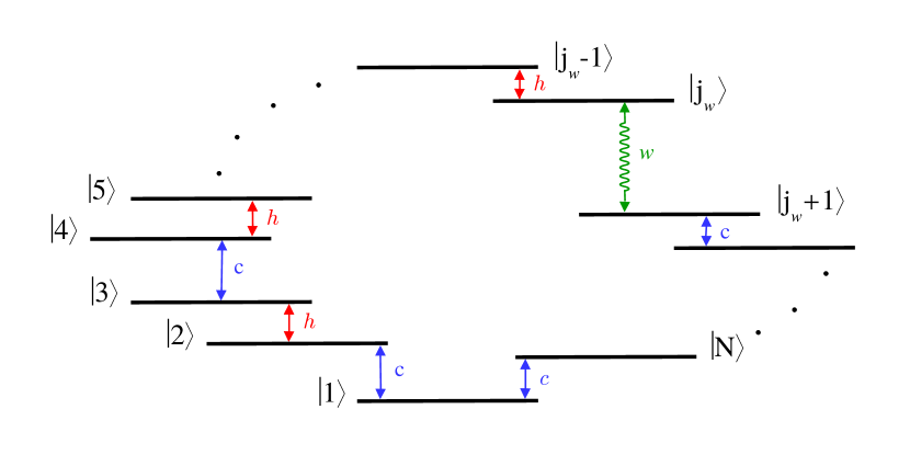
Figure 1: (colour online) Energy level diagram for a generic $N$-level cyclic thermal machine. The labelled red and blue arrows stands for transitions mediated by dissipative interactions with the hot and cold bath, respectively. Their distribution is arbitrary. The periodic field coupling energy levels $\left|j_{w}\right\rangle$ and $\left|j_{w}+1\right\rangle$ is indicated by the wobbly green arrow.

We start by introducing the general model for a coherent cyclic thermal machine (see Fig. 1). The Hamiltonian for the system or working substance $S$ is comprised of two terms: a bare (time-independent) Hamiltonian $\hat{H}_{\text{0}}$ and a time-dependent contribution $\hat{H}_{\text{d}}(t)$ which describes the coupling to a sinusoidal driving field. That is,

$$\hat{H}_{\text{s}}(t) = \hat{H}_{\text{0}}+\hat{H}_{\text{d}}(t),$$ (1a)

$$\hat{H}_{\text{0}} = \sum\nolimits_{i=1}^{N}E_{i}\,|i\rangle\langle i|,$$ (1b)

$$\hat{H}_{\text{d}}(t) = 2\hbar\lambda\left|j_{w}\right\rangle\left\langle j_{w}+1\right|\cos{\omega_{j_{w}}\,t}+\text{h.c.},$$ (1c)

where $\hbar$ is the reduced Planck constant and $\lambda$ controls the strength of the interaction with the field. $E_{i}$ and $\left|i\right\rangle$ are, respectively, the energies and eigenstates of the bare Hamiltonian. In particular, the driving connects the bare energy states $\left|j_{w}\right\rangle$ and $\left|j_{w}+1\right\rangle$. For simplicity, we assume a resonant coupling, i.e., $\omega_{j_{w}}\coloneqq(E_{j_{w}+1}-E_{j_{w}})/\hbar$, which is optimal from a thermodynamic viewpoint. The generalization to the non-resonant case is, nevertheless, straightforward.

The hot and cold bath can be cast as infinite collections of independent bosonic modes with a well-defined temperature. Their Hamiltonians read

$$\hat{H}_{\alpha}=\hbar\sum\nolimits_{\mu}\omega_{\mu,\alpha}\,\hat{b}_{\mu,\alpha}^{\dagger}\hat{b}_{\mu,\alpha},\qquad\alpha\in\{c,h\},$$ (2)

with $\hat{b}_{\mu,\alpha}^{\dagger}$ and $\hat{b}_{\mu,\alpha}$ being the bosonic creation and annihilation operators of the mode at frequency $\omega_{\mu,\alpha}$ in bath $\alpha\in\{c,h\}$. For the system-baths couplings, we adopt the general form $\hat{H}_{\text{s--$\alpha$}}=\hat{X}_{\alpha}\otimes\hat{B}_{\alpha}$, where

$$\hat{X}_{\alpha} = \sum\nolimits_{i\in\mathbf{R}_{\alpha}}\left|i\right\rangle\left\langle i+1\right|+\text{h.c.},$$ (3a)

$$\hat{B}_{\alpha} = \hbar\sqrt{\gamma_{\alpha}}\sum\nolimits_{\mu}g_{\mu,\alpha}\,\left(\hat{b}_{\mu,\alpha}+\hat{b}_{\mu,\alpha}^{\dagger}\right).$$ (3b)

Here, $g_{\mu,\alpha}\propto\sqrt{\omega_{\mu,\alpha}}$ and $\gamma_{\alpha}$ is the dissipation rate for bath $\alpha$. $\mathbf{R}_{\alpha}$ stands for the labels of the eigenstates $\left|i\right\rangle$ dissipatively coupled to $\left|i+1\right\rangle$ through the interaction with bath $\alpha$. For instance, in Fig. 1, $\mathbf{R}_{c}=\{1,3,\ldots,j_{w}+1,\ldots,N\}$ and $\mathbf{R}_{h}=\{2,4,\ldots,j_{w}-1,\ldots\}$. Notice that all levels $\left|i\right\rangle$ are thermally coupled to $\left|i+1\right\rangle$ (provided that $i\neq j_{w}$) via either the hot or the cold bath. In particular, the $N$-th level couples to $i=1$, hence closing the cycle. Without loss of generality, we consider that all transitions related to the same bath have different energy gaps, i.e., $|\omega_{k}|\neq|\omega_{l}|$ for $k,\,l\in\mathbf{R}_{\alpha}$ ($k\neq l$). This technical assumption simplifies the master equation but does not restrict the physics of the problem. The full Hamiltonian of the setup is thus

$$\hat{H}=\hat{H}_{\text{s}}+\sum\nolimits_{\alpha}\hat{H}_{\text{s--$\alpha$}}+\hat{H}_{\alpha}.$$ (4)

Although we consider a cyclic scheme of transitions, our formalism applies to more general quantum-coherent heat devices. Namely, equivalent results can be easily found for non-degenerate systems with various non-consecutive driven transitions. Likewise, one could include parasitic loops to the design. As an illustration, we analyze a model including an extra hot transition between $\left|j_{w}\right\rangle$ and $\left|j_{w}+1\right\rangle$ in the Appendix below.

II.2 The local master equation for weak driving

When deriving an effective equation of motion for the system, it is important to consider the various time scales involved Breuer and Petruccione (2002). Namely, the bath correlation time $\tau_{\text{B}}$, the intrinsic time scale of the bare system $\tau_{\text{0}}$, the relaxation time scale $\tau_{\text{R}}$, and the typical time associated with the interaction of the bare system with the external field $\tau_{\text{s--d}}$. These are

$$\tau_{\text{B}} \simeq\max\big{\{}\,\hbar/(k_{B}T_{\text{c}}),\,\hbar/(k_{B}T_{\text{h}})\,\big{\}}=\hbar/(k_{B}T_{\text{c}}).$$ (5a)

$$\tau_{\text{0}} \simeq\max\big{\{}\,|\pm\omega_{k}\mp\omega_{l}|^{-1},|2\,\omega_{k}|^{-1}\big{\}},\qquad(k\neq l).$$ (5b)

$$\tau_{\text{R}} \simeq\gamma_{\alpha}^{-1},\qquad\alpha\in\{c,h\}.$$ (5c)

$$\tau_{\text{s--d}} \simeq\lambda^{-1}.$$ (5d)

For a moment, let us switch off the time-dependent term $\hat{H}_{\text{d}}(t)$ and discuss the usual weak-coupling Markovian master equation, i.e., the Gorini–Kossakowski–Lindblad–Sudarshan (GKLS) equation Gorini et al. (1976); Lindblad (1976). Its microscopic derivation relies on the Born-Markov and secular approximations, which hold whenever $\tau_{\text{B}}\ll\tau_{\text{R}}$ and $\tau_{\text{0}}\ll\tau_{\text{R}}$. It can be written as

$$\frac{\mathop{}\!\mathrm{d}\hat{\rho}_{\text{s}}}{\mathop{}\!\mathrm{d}t}=-\frac{\mathrm{i}}{\hbar}[\hat{H}_{\text{0}},\,\hat{\rho}_{\text{s}}]+\left(\pazocal{L}_{\text{c}}+\pazocal{L}_{\text{h}}\right)\,\hat{\rho}_{\text{s}},$$ (6)

where $\hat{\rho}_{\text{s}}$ is the reduced state of the $N$-level system. Crucially, due to the underlying Born approximation of weak dissipation, Eq. (6) is correct only to $\pazocal{O}\big{(}\max\{\gamma_{\text{c}},\gamma_{\text{h}}\}\big{)}$.

The action of the super-operator $\pazocal{L}_{\alpha}$ is given by

$$\pazocal{L}_{\alpha}\,\hat{\rho}_{\text{s}}=\sum\nolimits_{i\in\mathbf{R}_{\alpha}}\Gamma_{\omega_{i}}^{\alpha}\,\bigg{(}\hat{A}_{i}\,\hat{\rho}_{\text{s}}\hat{A}_{i}^{\dagger}-\frac{1}{2}\left\{\hat{A}_{i}^{\dagger}\hat{A}_{i},\,\hat{\rho}_{\text{s}}\right\}_{+}\bigg{)}\\ +\Gamma_{-\omega_{i}}^{\alpha}\,\bigg{(}\hat{A}_{i}^{\dagger}\hat{\rho}_{S}\hat{A}_{i}-\frac{1}{2}\left\{\hat{A}_{i}\,\hat{A}_{i}^{\dagger},\,\hat{\rho}_{\text{s}}\right\}_{+}\bigg{)}.$$ (7)

Here, $\hat{A}_{i}=\left|i\right\rangle\left\langle i+1\right|$ and the notation $\{\cdot,\cdot\}_{+}$ stands for anti-commutator. The ‘jump’ operators $\hat{A}_{i}$ are such that $\hat{X}_{\alpha}=\sum\nolimits_{i\in\mathbf{R}_{\alpha}}\big{(}\hat{A}_{i}+\hat{A}_{i}^{\dagger}\big{)}$ and $[\hat{H}_{\text{0}},\hat{A}_{i}]=-\omega_{i}\hat{A}_{i}$. As a result, the operators $\hat{X}_{\alpha}$ in the interaction picture with respect to $\hat{H}_{\text{0}}$ read

$$e^{\mathrm{i}\,\hat{H}_{\text{0}}\,t/\hbar}\,\hat{X}_{\alpha}\,e^{-\mathrm{i}\,\hat{H}_{\text{0}}\,t/\hbar}=\sum\nolimits_{i\in\mathbf{R}_{\alpha}}e^{-\mathrm{i}\,\omega_{i}\,t}\hat{A}_{i}.$$ (8)

This identity is a key step in the derivation of Eq. (6) Breuer and Petruccione (2002).

If we now switch $\hat{H}_{\text{d}}(t)$ back on, we will need to change the propagator in Eq. (8) over to the time-ordered exponential

$$\hat{U}_{\text{s}}(t)=\pazocal{T}\,\exp{\left(-\mathrm{i}\,\hbar^{-1}\int_{0}^{t}\mathop{}\!\mathrm{d}t^{\prime}\,[\,\hat{H}_{\text{0}}+\hat{H}_{\text{d}}(t^{\prime})\,]\,\right)}.$$ (9)

When deriving a GKLS master equation for such a periodically driven system one also looks for a different decomposition on the right-hand side of Eq. (8) Alicki et al. ; Szczygielski (2014); Correa et al. (2014b). Namely,

$$\hat{U}_{\text{s}}^{\dagger}(t)\,\hat{X}_{\alpha}\,\hat{U}_{\text{s}}(t)=\sum\nolimits_{q\in\mathbb{Z}}\sum\nolimits_{\{\bar{\omega}\}}e^{-\mathrm{i}\,(\bar{\omega}+q\,\omega_{j_{w}})\,t}\hat{A}_{i}^{(q)}.$$ (10)

We will skip all the technical details and limit ourselves to note that if, in addition to $\tau_{\text{B}}\ll\tau_{\text{R}}$ and $\tau_{\text{0}}\ll\tau_{\text{R}}$, we make the weak driving assumption of $\tau_{\text{R}}\ll\tau_{\text{s--d}}$, Eq. (10) can be cast as

$$\hat{U}_{\text{s}}^{\dagger}(t)\,\hat{X}_{\alpha}\,\hat{U}_{\text{s}}(t) =e^{\mathrm{i}\,\hat{H}_{\text{0}}\,t/\hbar}\,\hat{X}_{\alpha}\,e^{-\mathrm{i}\,\hat{H}_{\text{0}}\,t/\hbar}+\pazocal{O}(\lambda)$$

$$=\sum\nolimits_{i\in\mathbf{R}_{\alpha}}e^{-\mathrm{i}\,\omega_{i}\,t}\hat{A}_{i}+\pazocal{O}(\lambda).$$ (11)

This is due to the fact that $\hat{H}_{\text{d}}$ is $\pazocal{O}(\lambda)$ while $\hat{H}_{\text{0}}$ is $\pazocal{O}(1)$. Exploiting Eq. (11) and following the exact same standard steps that lead to Eq. (6), one can easily see that the master equation

$$\frac{\mathop{}\!\mathrm{d}\hat{\rho}_{\text{s}}}{\mathop{}\!\mathrm{d}t}=-\frac{\mathrm{i}}{\hbar}[\hat{H}_{\text{0}}+\hat{H}_{\text{d}}(t),\,\hat{\rho}_{\text{s}}]+\left(\pazocal{L}_{\text{c}}+\pazocal{L}_{\text{h}}\right)\,\hat{\rho}_{\text{s}}$$ (12)

would hold up to $\pazocal{O}(\lambda\max\{\gamma_{c},\gamma_{h}\})$.

Effectively, Eq. (12) assumes that the dissipation is entirely decoupled from the intrinsic dynamics of $S$, which includes the driving. This is reminiscent of the ‘local’ master equations which are customarily used when dealing with weakly interacting multipartite open quantum systems Wichterich et al. (2007); González et al. (2017a); Hofer et al. (2017). We want to emphasize that, just like we have done here, it is very important to establish precisely the range of validity of such local equations Trushechkin and Volovich (2016) since using them inconsistently can lead to violations of the laws of thermodynamics Levy and Kosloff (2014); Stockburger and Motz (2016).

It is convenient to move into the rotating frame $\hat{\rho}_{\text{s}}\mapsto e^{\mathrm{i}\,\hat{H}_{\text{0}}\,t/\hbar}\hat{\rho}_{\text{s}}e^{-\mathrm{i}\,\hat{H}_{\text{0}}\,t/\hbar}\coloneqq\hat{\sigma}_{\text{s}}$ in order to remove the explicit time dependence on the right-hand side of Eq. (12) and simplify the calculations. This gives

$$\frac{\mathop{}\!\mathrm{d}\hat{\sigma}_{\text{s}}}{\mathop{}\!\mathrm{d}t}=-\frac{\mathrm{i}}{\hbar}[\hat{h}_{\text{d}},\,\hat{\sigma}_{\text{s}}]+\left(\pazocal{L}_{c}+\pazocal{L}_{h}\right)\hat{\sigma}_{\text{s}},$$ (13)

where the Hamiltonian $\hat{H}_{\text{d}}(t)$ in the rotating frame is given by

$$\hat{h}_{\text{d}}\simeq\hbar\lambda\left(\left|j_{w}\right\rangle\left\langle j_{w}+1\right|+\text{h.c.}\right).$$ (14)

Here, we have neglected two fast-rotating terms, with frequencies $\pm 2\,\omega_{j_{w}}$. This is consistent with our weak driving approximation $\tau_{\text{s--d}}\gg\tau_{\text{R}}$, as all quantities here have been time-averaged over one period of the driving field.

The ‘decay rates’ $\Gamma_{\omega}^{\,\alpha}$ from Eq. (7) are the only missing pieces to proceed to calculate the thermodynamic variables in the non-equilibrium steady state of $S$. These are

$$\Gamma_{\omega}^{\,\alpha}=2\operatorname{Re}\,\int_{0}^{\infty}\mathop{}\!\mathrm{d}r~{}e^{\mathrm{i}\,\omega\,t}~{}{\rm Tr}\{\hat{B}_{\alpha}(t)\hat{B}_{\alpha}(t-r)\hat{\rho}_{\alpha}\},$$ (15)

where the operator $\hat{\rho}_{\alpha}$ represents the thermal state of bath $\alpha$. Assuming $d_{\alpha}$-dimensional baths with an infinite cutoff frequency, the decay rates become Breuer and Petruccione (2002)

$$\Gamma_{\omega}^{\,\alpha} = \gamma_{\alpha}\,(\omega/\omega_{0})^{d_{\alpha}}\,\left[1-\exp\left(-\hbar\omega/k_{B}T_{\alpha}\right)\right]^{-1},$$ (16a)

$$\Gamma_{-\omega}^{\,\alpha} = \exp{\left(-\hbar\omega/k_{B}T_{\alpha}\right)}\,\Gamma^{\,\alpha}_{\omega},$$ (16b)

with $\omega>0$. In our model, $\omega_{0}$ depends on the physical realization of the system-bath coupling. $d_{\alpha}=1$ would correspond to Ohmic dissipation and $d_{\alpha}=\{2,3\}$, to the super-Ohmic case.

II.3 Heat currents, power, and performance

As it is standard in quantum thermodynamics, we will use the master equation (13) to break down the average energy change of the bare system $\frac{\mathop{}\!\mathrm{d}}{\mathop{}\!\mathrm{d}t}\langle E\rangle(t)={\rm tr}\,\{\hat{H}_{\text{0}}\,\frac{\mathop{}\!\mathrm{d}}{\mathop{}\!\mathrm{d}t}\hat{\sigma}_{\text{s}}(t)\}$ into ‘heat’ and ‘power’ contributions [i.e., $\frac{\mathop{}\!\mathrm{d}}{\mathop{}\!\mathrm{d}t}\langle E\rangle(t)=\sum\nolimits_{\alpha}\dot{\mathscr{Q}}_{\alpha}(t)+\mathscr{P}(t)$]. These can be defined as Uzdin et al. (2015)

$$\dot{\mathscr{Q}}_{\alpha}(t) \coloneqq{\rm tr}\,\{\hat{H}_{\text{0}}\,\pazocal{L}_{\alpha}\,\hat{\sigma}_{\text{s}}(t)\},$$ (17a)

$$\mathscr{P}(t) \coloneqq-\mathrm{i}\,\hbar^{-1}{\rm tr}\,\{\hat{H}_{\text{0}}\,[\hat{h}_{\text{d}},\hat{\sigma}_{\text{s}}(t)]\}.$$ (17b)

In the long-time limit, $\frac{\mathop{}\!\mathrm{d}}{\mathop{}\!\mathrm{d}t}\langle E\rangle\xrightarrow[]{t\rightarrow\infty}0$, and we will denote the corresponding steady-state heat currents and stationary power input by $\dot{\mathscr{Q}}_{\alpha}$ and $\mathscr{P}$, respectively. In particular, from Eqs. (7) and (17) it can be shown that Alicki (1979); Spohn (1978)

$$\dot{\mathscr{Q}}_{c}+\dot{\mathscr{Q}}_{h}+\mathscr{P} =0,$$ (18a)

$$\frac{\dot{\mathscr{Q}}_{c}}{T_{c}}+\frac{\dot{\mathscr{Q}}_{h}}{T_{h}} \leq 0,$$ (18b)

which amount to the First and Second Law of thermodynamics. It is important to note that the strict negativity of Eq. (18b) follows directly from the geometric properties of the dynamics generated by the local dissipators $\pazocal{L}_{\alpha}$ Spohn (1978). Working with any other reference frame to quantify energy exchanges in Eqs. (17), such as, e.g., $\hat{H}_{0}+\hat{h}_{\text{d}}$, would lead to undesirable violations of the Second Law Levy and Kosloff (2014). We thus see that the choice of the eigenstates of the bare Hamiltonian as preferred basis has a sound thermodynamic justification.

Using Eqs. (1b), (7), (14), and (17), we find for our cyclic $N$-level model

$$\dot{\mathscr{Q}}_{\alpha} = \sum\nolimits_{i\in R_{\alpha}}(E_{i+1}-E_{i})\,J_{i}\,,$$ (19a)

$$\mathscr{P} = 2\hbar\lambda\,\omega_{j_{w}}\,\operatorname{Im}\,\left\langle j_{w}\right|\hat{\sigma}_{\text{s}}(\infty)\left|j_{w}+1\right\rangle,$$ (19b)

where $J_{i}=\Gamma_{-\omega_{i}}^{\,\alpha_{i}}\,p_{i}^{(\infty)}-\Gamma_{\omega_{i}}^{\,\alpha_{i}}\,p_{i+1}^{(\infty)}$ is the net stationary transition rate from $\left|i\right\rangle$ to $\left|i+1\right\rangle$ and $p_{i}^{(\infty)}\coloneqq\left\langle i\,\right|\hat{\sigma}_{\text{s}}(\infty)\left|\,i\right\rangle$. The super-index $\alpha_{i}$ stands for the bath associated with the dissipative transition $\left|i\right\rangle\leftrightarrow\left|i+1\right\rangle$. Crucially, Eq. (19b) implies that vanishing stationary quantum coherence results in vanishing power consumption ($\mathscr{P}=0$) and hence, no refrigeration (see also, e.g., Ref. Kosloff and Levy (2014)). In fact, as we shall see below, $\dot{\mathscr{Q}}_{\alpha}=0$ in absence of coherence. Therefore, our cyclic model in Fig. 1 is inherently quantum since it requires non-zero coherences to operate.

II.4 Steady-state populations and coherence

The key to understand why our weakly driven cyclic devices can be emulated classically resides in the interplay between populations and coherence in the eigenbasis $\{\left|i\right\rangle\}_{i=1}^{N}$ of the bare Hamiltonian $\hat{H}_{\text{0}}$. In this representation, Eq. (13) reads:

$$\frac{\mathop{}\!\mathrm{d}p_{i}}{\mathop{}\!\mathrm{d}t}=\Gamma_{-\omega_{i-1}}^{\,\alpha_{i-1}}p_{i-1}-\left(\Gamma_{\omega_{i-1}}^{\,\alpha_{i-1}}+\Gamma_{-\omega_{i}}^{\,\alpha_{i}}\right)\,p_{i}+\Gamma_{\omega_{i}}^{\,\alpha_{i}}\,p_{i+1},$$ (20a)

$$\frac{\mathop{}\!\mathrm{d}p_{j_{w}}}{\mathop{}\!\mathrm{d}t}=\Gamma_{-\omega_{{j_{w}}-1}}^{\,\alpha_{{j_{w}}-1}}p_{{j_{w}}-1}-\Gamma_{\omega_{{j_{w}}-1}}^{\,\alpha_{{j_{w}}-1}}\,p_{j_{w}}-2\lambda\,\operatorname{Im}\,\left\langle{j_{w}}\right|\hat{\sigma}_{\text{s}}\left|{j_{w}}+1\right\rangle,$$ (20b)

$$\frac{\mathop{}\!\mathrm{d}p_{{j_{w}}+1}}{\mathop{}\!\mathrm{d}t}=\Gamma_{\omega_{{j_{w}}+1}}^{\,\alpha_{{j_{w}}+1}}\,p_{{j_{w}}+2}-\Gamma_{-\omega_{{j_{w}}+1}}^{\,\alpha_{{j_{w}}+1}}p_{{j_{w}}+1}+2\lambda\,\operatorname{Im}\,\left\langle{j_{w}}\right|\hat{\sigma}_{\text{s}}\left|{j_{w}}+1\right\rangle,$$ (20c)

for $i\neq\{{j_{w}},{j_{w}}+1\}$. Note that we have omitted the time labels in $p_{k}=\left\langle k\right|\hat{\sigma}_{\text{s}}(t)\left|k\right\rangle$ for brevity. Importantly, the populations of the pair of levels coupled to the driving field do depend on the coherence between them. In turn, this coherence evolves as

$$\frac{\mathop{}\!\mathrm{d}}{\mathop{}\!\mathrm{d}t}\left\langle{j_{w}}\right|\hat{\sigma}_{\text{s}}\left|{j_{w}}+1\right\rangle\\ =-\frac{1}{2}\left(\Gamma_{\omega_{{j_{w}}-1}}^{\,\alpha_{{j_{w}}-1}}+\Gamma_{-\omega_{{j_{w}}+1}}^{\,\alpha_{{j_{w}}+1}}\right)\,\left\langle{j_{w}}\right|\hat{\sigma}_{\text{s}}\left|{j_{w}}+1\right\rangle-\mathrm{i}\lambda\left(p_{{j_{w}}+1}-p_{j_{w}}\right).$$ (21)

Hence, the steady-state coherence (i.e., $\frac{\mathop{}\!\mathrm{d}}{\mathop{}\!\mathrm{d}t}\left\langle{j_{w}}\right|\hat{\sigma}_{\text{d}}\left|{j_{w}}+1\right\rangle_{\infty}\coloneqq 0$) in the subspace spanned by $\left|{j_{w}}\right\rangle$ and $\left|{j_{w}}+1\right\rangle$ is given in terms of the steady-state populations only. Namely, as

$$\left\langle{j_{w}}\right|\hat{\sigma}_{\text{s}}\left|{j_{w}}+1\right\rangle_{\infty}=\mathrm{i}\frac{2\lambda\,\left(p_{{j_{w}}}^{(\infty)}-p_{{j_{w}}+1}^{(\infty)}\right)}{\Gamma_{\omega_{{j_{w}}-1}}^{\,\alpha_{{j_{w}}-1}}+\Gamma_{-\omega_{{j_{w}}+1}}^{\,\alpha_{{j_{w}}+1}}}.$$ (22)

Inserting Eq. (22) in (20) and imposing $\frac{\mathop{}\!\mathrm{d}}{\mathop{}\!\mathrm{d}t}p_{k}^{(\infty)}=0$ yields a linear system of equations for the $N$ stationary populations $\mathbf{p}_{\infty}\coloneqq\big{(}p_{1}^{(\infty)},p_{2}^{(\infty)},\ldots,p_{N}^{(\infty)}\big{)}^{\mathsf{T}}$. This can be cast as $\mathbf{W}\,\mathbf{p}_{\infty}=0$, where the non-zero elements of the ‘matrix of rates’ $\mathbf{W}$ are

$$\begin{split}W_{i,\,i+1}&=\Gamma_{\omega_{i}}^{\,\alpha_{i}},\,W_{i+1,\,i}=\Gamma_{-\omega_{i}}^{\,\alpha_{i}},\\ W_{i,\,i-1}&=\Gamma_{-\omega_{i-1}}^{\,\alpha_{i-1}},\,W_{i-1,\,i}=\Gamma_{\omega_{i-1}}^{\,\alpha_{i-1}},\\ W_{i,\,i}&=-\,\left(\Gamma_{\omega_{i-1}}^{\,\alpha_{i-1}}+\Gamma_{-\omega_{i}}^{\,\alpha_{i}}\right),\end{split}$$ (23)

for $i\neq\{{j_{w}},{j_{w}}+1\}$, and

$$\begin{split}W_{{j_{w}},\,{j_{w}}+1}&=W_{{j_{w}}+1,\,{j_{w}}}=4\,\lambda^{2}\left[\Gamma_{\omega_{{j_{w}}-1}}^{\,\alpha_{{j_{w}}-1}}+\Gamma_{-\omega_{{j_{w}}+1}}^{\,\alpha_{{j_{w}}+1}}\right]^{-1},\\ W_{{j_{w}},\,{j_{w}}}&=-\left(\Gamma_{\omega_{{j_{w}}-1}}^{\,\alpha_{{j_{w}}-1}}+W_{{j_{w}},\,{j_{w}}+1}\right),\\ W_{{j_{w}}+1,\,{j_{w}}+1}&=-\left(\Gamma_{-\omega_{{j_{w}}+1}}^{\,\alpha_{{j_{w}}+1}}+W_{{j_{w}},\,{j_{w}}+1}\right).\end{split}$$ (24)

Note that, even if $\mathbf{W}\,\mathbf{p}_{\infty}=0$ (together with the normalization condition) determines the stationary populations of our model, Eqs. (20) certainly differ from

$$\frac{\mathop{}\!\mathrm{d}\mathbf{q}(t)}{\mathop{}\!\mathrm{d}t}=\mathbf{W}\,\mathbf{q}(t).$$ (25)

That is, the $\mathbf{q}(t)$ defined by Eq. (25) converges to $\mathbf{p}_{\infty}$ asymptotically but it does not coincide with $\big{(}p_{1}(t),\cdots p_{N}(t)\big{)}^{\mathsf{T}}$ at any finite time. Nonetheless, as we shall argue below, a classical system $S^{\prime}$ made up of $N$ discrete states evolving as per Eq. (25) can emulate the steady-state energy conversion process of the quantum-coherent system $S$. Note that a similar trick has been used in Holubec and Novotnỳ (2018), for an absorption refrigerator model where coherences appear accidentally, due to degeneracy. In contrast, as argued in Sec. II.3, the quantum coherence in our model is instrumental for its operation.

Remarkably, an equation similar to (25) can be found for an arbitrary choice of basis. Crucially, however, the physically motivated choice of the eigenbasis of $\hat{H}_{0}$ ensures the positivity of all non-diagonal rates in $\mathbf{W}$, that they obey detailed balance relations [cf. Eqs. (26) below], and the structure of Eq. (19a). All these are necessary conditions for building a classical emulator for the energy-conversion process, as we show below.

III Classical emulators

III.1 General properties

Let us now discuss in detail the properties of the emulator $S^{\prime}$ as defined by Eq. (25). First of all, note that (25) is a proper balance equation since: (i) the non-diagonal elements of $\mathbf{W}$ are positive, (ii) the pairs $\{W_{i,\,i+1},\,W_{i+1,\,i}\}$ satisfy the detailed balance relations [cf. Eqs. (16b), (23), and (24)]

$$\frac{W_{i+1,\,i}}{W_{i,\,i+1}} =\exp\left(-\frac{\hbar\omega_{i}}{k_{B}T_{\alpha_{i}}}\right),\qquad(i\neq{j_{w}})$$ (26a)

$$\frac{W_{{j_{w}}+1,\,{j_{w}}}}{W_{{j_{w}},\,{j_{w}}+1}} =1,$$ (26b)

and (iii) the sum over columns in $\mathbf{W}$ is zero (i.e., $W_{k,\,k}=-\sum_{l\neq k}W_{l,\,k}$), reflecting the conservation of probability. This also implies that $\mathbf{W}$ is singular and that $\mathbf{p}_{\infty}$ is given by its non-vanishing off-diagonal elements.

Notice as well that rates like $\{W_{i,\,i+1},\,W_{i+1,\,i}\}_{i\neq{j_{w}}}$ in Eq. (26) can always be attributed to excitation/relaxation processes (across a gap $\hbar\omega_{i}$) mediated by a heat bath at temperature $T_{\alpha_{i}}$. On the contrary, $\{W_{{j_{w}},\,{j_{w}}+1},\,W_{{j_{w}}+1,{j_{w}}}\}$ indicate saturation. Therefore, one possible physical implementation of $S^{\prime}$ would be an $N$-state quantum system connected via suitably chosen coupling strengths to a hot and a cold bath as well as to a work repository, such as an infinite-temperature heat bath. Indeed, looking back at Eqs. (23), we see that the rates for the dissipative interactions in $S^{\prime}$ are identical to those in $S$. However, according to Eq. (24), the coupling to the driving is much smaller in the emulator than in the original quantum-coherent model. Hence, $S^{\prime}$ is not the result of dephasing the $N$-level cyclic machine, but a different device.

At this point, we still need to show that the steady-state energy fluxes of our emulator actually coincide with Eqs. (19). To do so, we now build a classical representation of $S^{\prime}$ based on graph theory. Importantly, this also serves as the generic physical embodiment for the emulator.

III.2 Graph representation and thermodynamic variables

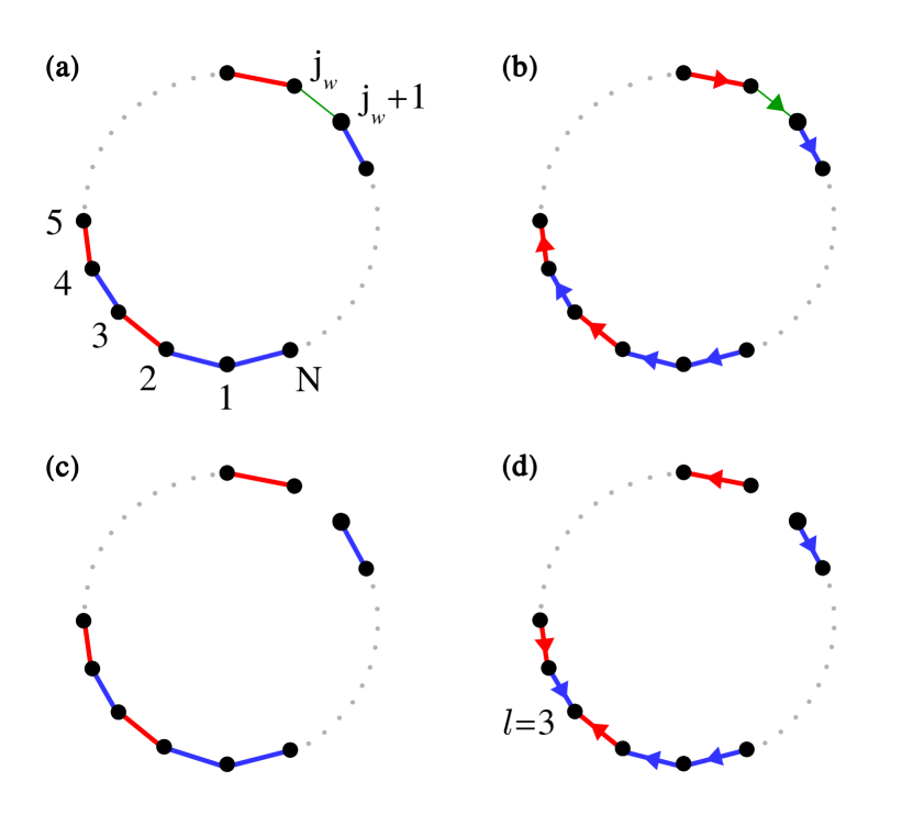
Figure 2: (colour online) (a) The circuit graph $\pazocal{C}_{N}$ is a classical emulator for the steady state of the $N$-level quantum-coherent device of Fig. 1. The blue edges are associated with dissipative transitions mediated by the cold bath. Similarly, the red edges and the green edge relate to the hot bath and the external driving. (b) When orienting the edges of $\pazocal{C}_{N}$ clockwise, the cycle $\vec{\pazocal{C}}_{N}$ is obtained. (c) Removing the edge $({j_{w}},{j_{w}}+1)$ from $\pazocal{C}_{N}$ yields the maximal tree $\pazocal{T}_{j_{w}}$. (d) Orienting $\pazocal{T}_{j_{w}}$ towards, e.g., vertex $l=3$ gives the oriented maximal tree $\vec{\pazocal{T}}_{j_{w}}^{\,l}$.

Using graph theory for the thermodynamic analysis of a system described by a set of rate equations has two major advantages: First, it provides a clear interpretation of the underlying energy conversion mechanisms González et al. (2016) and, secondly, it allows for the calculation of the thermodynamic variables directly from the matrix of rates Hill (1966). In fact, the graph itself also follows from $\mathbf{W}\$—each state $k=\{1,2,\ldots,N\}$ becomes a ‘vertex’ and each pair of non-vanishing rates $\{W_{k,\,l},\,W_{l,\,k}\}_{k\neq l}$ becomes an ‘undirected edge’ $(k,l)$ connecting $k$ and $l$. Specifically, this mapping would take Eq. (25) into the ‘circuit graph’ $\pazocal{C}_{N}$ depicted in Fig. 2(a). We can thus think of $S^{\prime}$ as a classical device transitioning cyclically between $N$ states.

Now that we have a physical picture in mind, we show that such classical emulator is thermodynamically equivalent to the coherent $N$-level machine, once in its steady state. Specifically, we focus on rewriting the thermodynamic variables of $S$ [cf. Eqs. (19)] in terms of elements of $S^{\prime}$. To that end, some graph objects need to be introduced. For instance, the undirected graph $\pazocal{C}_{N}$ may be oriented (or directed) either clockwise or anticlockwise, leading to the ‘cycles’ $\vec{\pazocal{C}}_{N}$ and $-\vec{\pazocal{C}}_{N}$, respectively [see Fig. 2(b)]. We may want to eliminate an edge from $\pazocal{C}_{N}$, e.g., $(k,k+1)$; the resulting undirected graph would be the ‘maximal tree’ $\pazocal{T}_{k}$ [see Fig. 2(c)]. Maximal trees can also be oriented towards a vertex, e.g., $l$; the corresponding graph would then be denoted by $\vec{\pazocal{T}}_{k}^{\,l}$ [see Fig. 2(d)]. Finally, if the edge $(k,l)$ is directed, e.g., from vertex $k$ to vertex $l$, we may pair it with the transition rate $W_{l,k}$. Similarly, any directed subgraph $\vec{\pazocal{G}}$, for example the cycle $\vec{\pazocal{C}}_{N}$ or the oriented maximal tree $\vec{\pazocal{T}}_{k}^{\,l}$, can be assigned a numeric value $\pazocal{A}(\vec{\pazocal{G}})$ given by the product of the transition rates of its directed edges. In particular, $\pazocal{A}(\vec{\pazocal{C}}_{N})=\Pi_{n=1}^{N}W_{n+1,\,n}$, $\pazocal{A}(-\vec{\pazocal{C}}_{N})=\Pi_{n=1}^{N}W_{n,\,n+1}$ and

$$\pazocal{A}(\vec{\pazocal{T}}_{k}^{\,l})=\left\{\begin{array}[]{lcc}\Pi_{n=1}^{l-1}W_{n+1,\,n}\ \Pi_{n=l+1}^{k}W_{n-1,\,n}\ \Pi_{n=k+1}^{N}W_{n+1,\,n}&l<k\\ \\ \Pi_{n=1}^{k-1}W_{n,\,n+1}\ \Pi_{n=k+1}^{l-1}W_{n+1,\,n}\ \Pi_{n=l}^{N}W_{n,\,n+1}&l>k+1\\ \\ \Pi_{n=1}^{k-1}W_{n+1,\,n}\ \Pi_{n=k+1}^{N}W_{n+1,\,n}&l=k\\ \\ \Pi_{n=1}^{k-1}W_{n,\,n+1}\ \Pi_{n=k+1}^{N}W_{n,\,n+1}&l=k+1\\ \end{array}\right.$$ (27)

where $W_{N,\,N+1}\equiv W_{N,\,1}$ and $W_{N+1,\,N}\equiv W_{1,\,N}$.

Our aim is to cast $\dot{\mathscr{Q}}_{\alpha}$ and $\mathscr{P}$ solely as functions of graph objects referring to $\pazocal{C}_{N}$. Let us start by noting that, the steady state populations $p_{i}^{(\infty)}$ of $S$ can be written as Schnakenberg (1976)

$$p_{i}^{(\infty)}=\pazocal{D}(\pazocal{C}_{N})^{-1}\sum\nolimits_{k=1}^{N}\pazocal{A}(\vec{\pazocal{T}}_{k}^{\,i}),$$ (28)

since, by definition, they coincide with those of $S^{\prime}$. Here, $\pazocal{D}(\pazocal{C}_{N})=\sum\nolimits_{k=1}^{N}\sum\nolimits_{l=1}^{N}\pazocal{A}(\vec{\pazocal{T}}_{k}^{\,l})$. Introducing Eq. (28) in the definition of $J_{i}$ [see text below Eqs. (19)], we get

$$J_{i}=\pazocal{D}(\pazocal{C}_{N})^{-1}\sum\nolimits_{k=1}^{N}\left[W_{i+1,\,i}\,\pazocal{A}(\vec{\pazocal{T}}_{k}^{\,i})-W_{i,\,i+1}\,\pazocal{A}(\vec{\pazocal{T}}_{k}^{\,i+1})\right].$$ (29)

The bracketed term in Eq. (29) turns out to be $\big{[}\pazocal{A}(\vec{\pazocal{C}}_{N})-\pazocal{A}(-\vec{\pazocal{C}}_{N})\big{]}\,\delta_{ki}$ González et al. (2017b), where $\delta_{ki}$ stands for the Kronecker delta. Therefore $J_{i}$ does not depend on $i$

$$J_{i}=\pazocal{D}(\pazocal{C}_{N})^{-1}\left[\pazocal{A}(\vec{\pazocal{C}}_{N})-\pazocal{A}(-\vec{\pazocal{C}}_{N})\right]\coloneqq J.$$ (30)

That is, in the steady state, the system exchanges energy with both baths and the driving field, with the same flux Schnakenberg (1976). This ‘tight-coupling’ condition between thermodynamic fluxes Esposito et al. (2009) implies that our $N$-level device is ‘endoreversible’ Correa et al. (2014b) and hence, that it can operate in the reversible limit of maximum energy-efficiency Correa et al. (2013).

As a result, Eq. (19a) becomes $\dot{\mathscr{Q}}_{\alpha}=J\sum\nolimits_{i\in\mathbf{R}_{\alpha}}(E_{i+1}-E_{i})$. Using (23) and (26a), we can see that

$$\sum\nolimits_{i\in R_{\alpha}}(E_{i+1}-E_{i})=-T_{\alpha}k_{B}\ln{\frac{\pazocal{A}^{\alpha}(\vec{\pazocal{C}}_{N})}{\pazocal{A}^{\alpha}(-\vec{\pazocal{C}}_{N})}}\coloneqq-T_{\alpha}\pazocal{X}^{\alpha}(\vec{\pazocal{C}}_{N}),$$ (31)

where $\pazocal{A}^{\alpha}(\pm\vec{\pazocal{C}}_{N})$ is the product of the rates of the directed edges in $\pm\vec{\pazocal{C}}_{N}$ associated with bath $\alpha$ only. Combining Eqs. (30) and (31), we can finally express the steady-state heat currents $\dot{\mathscr{Q}}_{\alpha}$ of the quantum-coherent $N$-level device $S$ as:

$$\dot{\mathscr{Q}}_{\alpha}=\frac{-T_{\alpha}\pazocal{X}^{\alpha}(\vec{\pazocal{C}}_{N})}{\pazocal{D}(\pazocal{C}_{N})}\left[\pazocal{A}(\vec{\pazocal{C}}_{N})-\pazocal{A}(-\vec{\pazocal{C}}_{N})\right]\equiv\dot{\mathscr{Q}}_{\alpha}(\pazocal{C}_{N}).$$ (32)

On the other hand, the power is easily calculated from energy conservation [cf. Eq. (18a)]. Remarkably, the right-hand side of Eq. (32) coincides with the steady-state heat currents of the circuit graph in Fig. 2(a), i.e., $\dot{\mathscr{Q}}_{\alpha}\equiv\dot{\mathscr{Q}}_{\alpha}(\pazocal{C}_{N})$ Hill (1966). Note that this is far from trivial, since (32) refers to $S$, even if written in terms of graph objects related to $S^{\prime}$. Therefore, we have shown that the $N$-level refrigerator and its classical emulator exhibit the same stationary heat currents and power consumption and are thus, thermodynamically indistinguishable. This is our main result. Note that the significance of Eq. (32) is not just that our model is classically emulable, but that it is classically emulable in spite of requiring quantum coherence to operate (cf. Sec. II.3).

III.3 Performance optimization of the thermal machine

The graph-theoretic expression (32) for the circuit currents of the classical emulator can also prove useful in the performance optimization of our quantum-coherent thermal machines $S$ González et al. (2017b). For instance, from the bracketed factor we see that the asymmetry in the stationary rates associated with opposite cycles is crucial in increasing the energy-conversion rate. On the other hand, the number of positive terms in the denominator scales as $\pazocal{D}(\pazocal{C}_{N})\sim N^{2}$, leading to vanishing currents. Therefore, larger energy-conversion rates are generally obtained in small few-level devices Correa (2014) featuring the largest possible asymmetry between opposite cycles.

Let us now focus on the refrigerator operation mode (i.e., $\dot{\mathscr{Q}}_{c}>0$, $\dot{\mathscr{Q}}_{h}<0$, and $\mathscr{P}>0$). Besides maximizing the cooling rate $\dot{\mathscr{Q}}_{c}$, it is of practical interest to operate at large ‘coefficient of performance’ (COP) $\pazocal{E}$, i.e., at large cooling per unit of supplied power. In particular, the COP writes as

$$\pazocal{E}\coloneqq\pazocal{E}\,(\pazocal{C}_{N})=\frac{\dot{\mathscr{Q}}_{c}(\pazocal{C}_{N})}{\mathscr{P}(\pazocal{C}_{N})}=\frac{-T_{c}\pazocal{X}^{c}(\vec{\pazocal{C}}_{N})}{T_{c}\pazocal{X}^{c}(\vec{\pazocal{C}}_{N})+T_{h}\pazocal{X}^{h}(\vec{\pazocal{C}}_{N})}.$$ (33)

As a consequence of the second law [cf. Eq. (18b)], $\pazocal{E}(\pazocal{C}_{N})$ is upper bounded by the Carnot COP ($\pazocal{E}_{C}$)

$$\pazocal{E}\,(\pazocal{C}_{N})\leq\pazocal{E}_{C}=\frac{T_{c}}{T_{h}-T_{c}}.$$ (34)

This limit would be saturated when $\pazocal{X}^{h}(\pazocal{C}_{N})=-\pazocal{X}^{c}(\pazocal{C}_{N})$ .

Since the coupling to the driving field sets the smallest energy scale in our problem, the corresponding transition rate normally satisfies $W_{{j_{w}},\,{j_{w}}+1}\ll W_{i,\,i+1}$, $\forall i\neq{j_{w}}$; unless some $\omega_{i}$ becomes very small. In turn, recalling the definition of an oriented maximal tree $\vec{\pazocal{T}}_{k}^{l}$ [see Fig. 2(d)], this implies $\big{\{}\pazocal{A}(\vec{\pazocal{T}}_{k}^{\,l})\big{\}}_{k\neq{j_{w}}}\ll\big{\{}\pazocal{A}(\vec{\pazocal{T}}_{j_{w}}^{\,l})\big{\}}_{l=1}^{N}$, since the latter do not contain the small factors $W_{{j_{w}},\,{j_{w}}+1}=W_{{j_{w}}+1,\,{j_{w}}}$, and allows for a convenient simplification of $\pazocal{D}(\pazocal{C}_{N})$ that we shall use below. Namely,

$$\pazocal{D}(\pazocal{C}_{N})=\left(\frac{\sum_{k\neq{j_{w}}}^{N}\sum\nolimits_{l=1}^{N}\pazocal{A}(\vec{\pazocal{T}}_{k}^{\,l})}{\sum\nolimits_{l=1}^{N}\pazocal{A}(\vec{\pazocal{T}}_{j_{w}}^{\,l})}+1\right)\,\sum\nolimits_{l=1}^{N}\pazocal{A}(\vec{\pazocal{T}}_{j_{w}}^{\,l})\\ \simeq\sum\nolimits_{l=1}^{N}\pazocal{A}(\vec{\pazocal{T}}_{j_{w}}^{\,l}).$$ (35)

IV Example: Power enhancement in a coherent four-level hybrid refrigerator

In this section we apply the above to a concrete example. Namely, we solve for the steady state of two models of quantum refrigerator and find that one of them is more energy-efficient and cools at a larger rate than the other provided its steady-state coherence is also larger. Moreover, the quantitative improvement in the cooling rate matches exactly the increase in steady-state coherence. As suggestive as this observation may seem, we then move on to show that quantum coherence is not indispensable to achieve such performance enhancement. We do so precisely by building classical emulators for both quantum-coherent models and observing that the exact same performance enhancement is possible within a fully classical stochastic-thermodynamic picture.

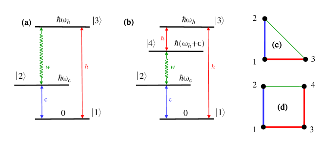
Figure 3: (colour online) (a) Three-level model. The system $S$ consists of three levels with energies $\{0,\,\hbar\omega_{c},\,\hbar\omega_{h}\}$, such that $0\leq\omega_{c}\leq\omega_{h}$. The dissipative transitions tagged $c$ and $h$ are mediated by a cold (blue arrow) and a hot bath (red arrow), respectively. The transition $w$ is driven by an external sinusoidal field (curly green arrow). (b) Four-level model. An extra level with energy $\hbar(\omega_{h}+\epsilon)$ is added to the three-level scheme. Note that $\epsilon$ can be positive or negative. The driving is now applied to the transition $\left|2\right\rangle\leftrightarrow\left|4\right\rangle$ and the new dissipative transition $\left|4\right\rangle\leftrightarrow\left|3\right\rangle$, due to the hot bath, is added to close the thermodynamic cooling cycle. The circuit graphs associated with the three and four-level models are depicted in panels (c) and (d), respectively. The thick blue (red) lines stand for dissipative transitions via the cold (hot) baths and the thin green lines, for the coupling to the driving.

IV.1 Performance advantage

Let us start by considering the three-level model depicted in Fig. 3(a). As we can see, this simple design consists of three states $\{\left|1\right\rangle,\left|2\right\rangle,\left|3\right\rangle\}$, with energies $\{0,\hbar\omega_{c},\hbar\omega_{h}\}$ connected through dissipative interactions with a cold and a hot bath (transitions $\left|1\right\rangle\leftrightarrow\left|2\right\rangle$ and $\left|1\right\rangle\leftrightarrow\left|3\right\rangle$, respectively), and the action of a weak driving field (transition $\left|2\right\rangle\leftrightarrow\left|3\right\rangle$).

It is then straightforward to find the steady-state $\hat{\sigma}_{\text{s}}(\infty)$ for the corresponding master equation (13), and use Eqs. (17) to compute the stationary heat currents $\dot{\mathscr{Q}}_{\alpha}^{\,(3)}$ and power consumption $\mathscr{P}^{\,(3)}$. It can be seen that the tight-coupling condition introduced in Sec. III.2 also applies to this case so that the coefficient of performance writes as

$$\pazocal{E}_{3}\coloneqq\frac{\dot{\mathscr{Q}}_{c}^{\,(3)}}{\mathscr{P}^{\,(3)}}=\frac{\omega_{c}}{\omega_{w}},$$ (36)

where $\omega_{w}\coloneqq\omega_{h}-\omega_{c}$.

We note that, when operating as a refrigerator, the three-level device uses the hot bath as a mere entropy sink; i.e., any excess heat is simply dumped into the hot bath and never reused. Interestingly, in order to improve the COP of actual (absorption) refrigerators it is commonplace to harness regenerative heat exchange in double-stage configurations. These recover waste heat from condensation to increase the evaporation rate of refrigerant Gordon and Ng (2000). Taking inspiration from thermal engineering, we thus add a fourth level $\left|4\right\rangle$ with energy $\hbar(\omega_{h}+\epsilon)$ as a stepping stone between $\left|2\right\rangle$ and $\left|3\right\rangle$. As shown in Fig. 3(b), we propose to use the external field only to drive the transition $\left|2\right\rangle\leftrightarrow\left|4\right\rangle$, with gap $\hbar(\omega_{w}+\epsilon)$. In order to close the thermodynamic cooling cycle, we put the hot bath to good use and connect dissipatively levels $\left|4\right\rangle$ and $\left|3\right\rangle$. This results in another tightly-coupled quantum refrigerator, with COP

$$\pazocal{E}_{4}\coloneqq\frac{\dot{\mathscr{Q}}_{c}^{\,(4)}}{\mathscr{P}^{\,(4)}}=\frac{\omega_{c}}{\omega_{w}+\epsilon}.$$ (37)

This is larger than $\pazocal{E}_{3}$ whenever $\epsilon<0$, as intended. For comparison, recall that quantum absorption refrigerators Palao et al. (2001) entirely replace the driving by a dissipative coupling to a third bath at temperature $T_{w}>T_{h}$. Our combined-cycle four-level model is therefore a novel hybrid design of independent interest, as it is partly driven by power and partly, by recovered waste heat.

IV.2 Power enhancement and quantum coherence

Even if the combined-cycle four-level refrigerator is more energy-efficient than its power-driven three-level counterpart, we do not know yet whether it can also cool at a faster rate. To see this, let us define the figure of merit $\mathscr{R}\coloneqq\dot{\mathscr{Q}}_{c}^{\,(4)}/\dot{\mathscr{Q}}_{c}^{\,(3)}$. From Eqs. (18a) and (19), it follows that

$$\mathscr{R}=\frac{C_{l_{1}}\left[\hat{\sigma}_{\text{s}}^{(4)}(\infty)\right]}{C_{l_{1}}\left[\hat{\sigma}_{\text{s}}^{(3)}(\infty)\right]},$$ (38)

where $C_{l_{1}}\big{[}\hat{\sigma}_{\text{s}}^{(N)}(\infty)\big{]}=\operatorname{Im}\,\left\langle j_{w}\right|\hat{\sigma}_{\text{s}}^{(N)}(\infty)\left|j_{w}+1\right\rangle$ stands for the $l_{1}$-norm of coherence Baumgratz et al. (2014); Streltsov et al. (2017) in the stationary state $\hat{\sigma}_{\text{s}}^{(N)}(\infty)$ of the $N$-level thermal machine. This is a bona fide quantifier of the amount of coherence involved in the steady-state operation of the device. An enhancement in the cooling rate translates into $\mathscr{R}>1$ and hence, is only possible if the steady state $\hat{\sigma}_{\text{s}}^{(4)}(\infty)$ of the four level device contains more quantum coherence than $\hat{\sigma}_{\text{s}}^{(3)}(\infty)$. As it turns out, it is rather easy to find parameter ranges in which $\mathscr{R}>1$, as shown in Figs. 4(a) and (b). Importantly, it is even possible to find parameters for which $\pazocal{E}_{4}>\pazocal{E}_{3}$ and $\dot{\mathscr{Q}}_{c}^{\,(4)}>\dot{\mathscr{Q}}_{c}^{\,(3)}$ simultaneously.

IV.3 Power enhancement without quantum coherence

Both the three and four-level refrigerators are cyclic non-degenerate heat devices and hence, classically emulable. In particular, the emulator for the three-level model is the triangle $\pazocal{C}_{3}$ depicted in Fig. 3(c) while the steady state of the hybrid four-level refrigerator is emulated by the square graph $\pazocal{C}_{4}$ of Fig. 3(d). In spite of the fact that there exist quantum coherent implementations of these energy-conversion cycles for which $\mathscr{R}>1\Leftrightarrow C_{l_{1}}\left[\hat{\sigma}_{\text{s}}^{(4)}(\infty)\right]>C_{l_{1}}\left[\hat{\sigma}_{\text{s}}^{(3)}(\infty)\right]$, it would be wrong to claim that quantumness is necessary for such performance boost—the corresponding emulators also satisfy $\dot{\mathscr{Q}}_{c}(\pazocal{C}_{4})=\dot{\mathscr{Q}}_{c}^{\,(4)}>\dot{\mathscr{Q}}_{c}(\pazocal{C}_{3})=\dot{\mathscr{Q}}_{c}^{\,(3)}$, and yet have no coherence.

IV.4 Analytical insights from graph theory

IV.4.1 Cooling rate

Using Eqs. (26a), (31)–(33), we readily find that

$$\dot{\mathscr{Q}}_{c}(\pazocal{C}_{3}) = \hbar\omega_{c}\frac{\pazocal{A}(\vec{\pazocal{C}}_{3})}{\pazocal{D}(\pazocal{C}_{3})}\left[1-\exp{\left(X_{c}-X_{h}\right)}\right].$$ (39a)

$$\dot{\mathscr{Q}}_{c}(\pazocal{C}_{4}) = \hbar\omega_{c}\frac{\pazocal{A}(\vec{\pazocal{C}}_{4})}{\pazocal{D}(\pazocal{C}_{4})}\left[1-\exp{\left(X_{c}-X_{h}-X_{\epsilon}\right)}\right].$$ (39b)

The quantities $X_{c}\coloneqq\hbar\omega_{c}/k_{B}T_{c}$, $X_{h}\coloneqq\hbar\omega_{h}/k_{B}T_{h}$, and $X_{\epsilon}\coloneqq\hbar\epsilon/k_{B}T_{h}$ are ‘thermodynamic forces’ associated with the cold and hot baths. Note that their difference encodes the asymmetry between the two possible orientations of the graphs.

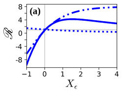
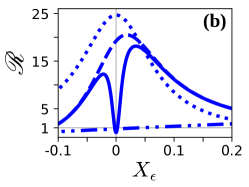
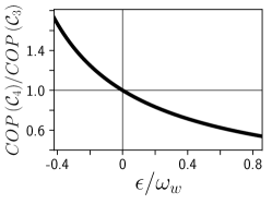
Figure 4: (colour online) (a) Performance ratio $\mathscr{R}=\dot{\mathscr{Q}}_{c}(\pazocal{C}_{4})/\dot{\mathscr{Q}}_{c}(\pazocal{C}_{3})$ (solid line) as a function of the thermodynamic force $X_{\epsilon}$. We also plot the approximation $AD$ from Eq. (40a) (dashed line), and the factors $A$ (dotted line) and $D$ (dot-dashed line). In this case, the solid and dashed lines are indistinguishable at the scale of the figure. We have chosen one-dimensional baths $d_{c}=d_{h}=1$, $\omega_{h}=1$, $\omega_{c}=0.3$, $\lambda=10^{-8}$, $\gamma_{c}=\gamma_{h}=10^{-6}$, $T_{c}=1.5$, and $T_{h}=3$ ($\hbar=k_{B}=1$). Importantly, as discussed in Sec. IV.2, $\mathscr{R}$ coincides with the ratio of stationary coherence of the four-level model and the benchmark, measured by the $l_{1}$-norm. (b) Same as in (a) for three-dimensional baths ($d_{c}=d_{h}=3$). The rest of parameters remain unchanged. (c) Ratio between the COPs of $\pazocal{C}_{3}$ and $\pazocal{C}_{4}$ versus $\epsilon$. Note that, for $\epsilon<0$, the four-level device can simultaneously achieve larger cooling power and COP. All parameters are the same as in (b).

IV.4.2 Performance enhancement

A manageable analytical approximation for the figure of merit $\mathscr{R}=\dot{\mathscr{Q}}_{c}(\pazocal{C}_{4})/\dot{\mathscr{Q}}_{c}(\pazocal{C}_{3})$ can be obtained by combining Eqs. (23), (24), (39a), and (39b) with the assumption that the smallest transition rate is the one related to the driving field [i.e., Eq. (35)]. This gives

$$\mathscr{R} \simeq AD,$$ (40a)

$$A \coloneqq\frac{1+\exp{\left(X_{c}\right)}+\exp{\left(X_{c}-X_{h}\right)}}{1+\exp{\left(X_{c}\right)}+\exp{\left(X_{c}-X_{h}\right)}+\exp{\left(X_{c}-X_{h}-X_{\epsilon}\right)}}$$

$$\qquad\qquad\qquad\qquad\qquad\times\frac{1-\exp{\left(X_{c}-X_{h}-X_{\epsilon}\right)}}{1-\exp{\left(X_{c}-X_{h}\right)}},$$ (40b)

$$D \coloneqq\frac{\Gamma_{\omega_{c}}^{c}+\Gamma_{\omega_{h}}^{h}}{\Gamma_{\omega_{c}}^{c}+\Gamma_{\epsilon}^{h}}.$$ (40c)

As we can see, the factor $A$ depends exclusively on the thermodynamic forces $X_{c}$, $X_{h}$ and $X_{\epsilon}$. Its second term describes the ratio between the cycles asymmetries. The new thermodynamic force allows for an additional control on the asymmetry of the four-level refrigerator, thus favouring the cooling cycle for $X_{\epsilon}>0$. In contrast, the quantity $D$ is purely dissipative; it encodes the ratio between the rates associated with the driving fields Eq. (24). Importantly, small $\epsilon$ in the four-level model can increase $D$. The choice of spectral density for the system-bath interactions (i.e., the dimensionality or ‘Ohmicity’ of the baths) can lead to a sufficiently large $D$ so that the product $\mathscr{R}=AD>1$ for $\epsilon<0$. Thus, factorizing $\mathscr{R}$ as in Eqs. (40) provides insights into the competing physical mechanisms responsible for the cooling power enhancements in the four-level device.

Fig. 4(a) illustrates how the approximation (40a) may hold almost exactly; namely, we work with one-dimensional baths ($d_{c}=d_{h}=1$) at moderate to large temperatures ($k_{B}T_{\alpha}/\hbar\omega_{\alpha}\gtrsim 1$). In this range of parameters, $A$ is the main contribution to the enhancement of $\dot{\mathscr{Q}}_{c}$, so that $\mathscr{R}$ is nearly insensitive to changes in the dissipation strengths.

On the contrary, when taking three-dimensional baths ($d_{c}=d_{h}=3$), the frequency-dependence of the transition rates is largely accentuated. At small $\epsilon$ the rate $W_{2,4}$ ceases to be the smallest in $\pazocal{C}_{4}$, which invalidates Eqs. (40) [see Fig. 4(b)] . In this case, the behaviour of $\mathscr{R}$ is dominated by $D$, and grows almost linearly with $\gamma_{h}$. Similar disagreements between $\mathscr{R}$ and the approximate formula Eq. (40) can be observed in the low-temperature regime.

As shown in Fig. 4(b), the hybrid four-level design can operate at much larger energy-conversion rates than the power-driven benchmark. Indeed, for the arbitrarily chosen parameters in the figure, $\dot{\mathscr{Q}}_{c}(\pazocal{C}_{4})$ can outperform $\dot{\mathscr{Q}}_{c}(\pazocal{C}_{3})$ by an order of magnitude at appropriate values of $\epsilon$. Such enhancement may be classically interpreted solely in terms of the asymmetry $A$ and the dissipation factor $D$, without resorting to the buildup of quantum coherence. Importantly, such qualitative understanding follows directly from the classical emulability of the model, which allows us to study the emulator in place of the original quantum-coherent device.

IV.4.3 Coefficient of performance and cooling window

The COPs of $\pazocal{C}_{3}$ and $\pazocal{C}_{4}$ are related through

$$\pazocal{E}\,(\pazocal{C}_{4})/\pazocal{E}\,(\pazocal{C}_{3})=(1+\epsilon/\omega_{w})^{-1}.$$ (41)

As already mentioned, $\epsilon<0$ results in an increase of the energetic performance of the four-level machine due to the lower power consumption [see Fig. 4(c)]. Interestingly, the ratio $\mathscr{R}$ can be larger than one for $\epsilon<0$, which entails a simultaneous power and efficiency enhancement. For instance, comparing Figs. 4(b) and 4(c), we observe increased power by a factor of $10$ together with a $10\%$ improvement in energy-efficiency.

On the other hand, the operation mode—heat engine or refrigerator—depends on the specific parameters of the models. In particular, to achieve cooling action in the three-level benchmark we must have $\dot{\mathscr{Q}}_{c}(\pazocal{C}_{3})>0$. According to Eq. (39a), this implies $X_{c}-X_{h}<0$ or, equivalently,

$$\omega_{c}<\omega_{c,\text{rev}}\coloneqq\omega_{h}\,T_{c}/T_{h}.$$ (42)

Taking a fixed $\omega_{h}$, the range of values $\omega_{c}<\omega_{c,\text{rev}}$ is thus referred-to as cooling window. On the other hand, from Eq. (39b) we can see that cooling is possible on $\pazocal{C}_{4}$ if

$$\omega_{c}<(\omega_{h}+\epsilon)\,T_{c}/T_{h}.$$ (43)

Hence, whenever $\epsilon>0$ the cooling window of the four-level model is wider than that of the benchmark for the same parameters $\omega_{h}$, $T_{\alpha}$, $\lambda$, $\gamma_{\alpha}$, and $d_{\alpha}$. Conversely, if we were interested in building a quantum heat engine, a negative $\epsilon$ [as depicted in Fig. 3(b)] would broaden the operation range.

V Conclusions

We have analyzed periodically driven thermal machines weakly coupled to an external field and characterized by a cyclic sequence of transitions. We have proposed a new approach to build fully incoherent classical emulators for this family of quantum-coherent heat devices, which exhibit the exact same thermodynamic operation in the long-time limit. In particular, we exploit the fact that the steady state of this type of coherent thermal machines coincides with that of some stochastic-thermodynamic model with the same number of states dissipatively connected via thermal coupling to the same heat baths, and obeying consistent rate equations.

We have then shown how the performance of a three-level quantum-coherent refrigerator may be significantly improved by driving it with a combination of waste heat and external power—both the energy-efficiency and the cooling rate can be boosted in this way. In particular, we have shown that the cooling enhancement is identical to the increase in stationary quantum coherence, when comparing our hybrid model with an equivalent benchmark solely driven by power. In spite of the close connection between the observed effects and the buildup of additional quantum coherence, we remark that these cannot be seen as unmistakable signatures of quantumness since our model belongs to the aforementioned family of “classically emulable” thermal machines.

In fact, the possibility to emulate clasically a quantum heat device goes far beyond the cyclic and weakly driven models discussed here. For instance, in the opposite limit of strong periodic driving (i.e., $\tau_{\text{d}}\ll\tau_{\text{R}}$) one can always resort to Floquet theory to map the steady state operation of the machine into a fully incoherent stochastic-thermodynamic process in some relevant rotating frame Alicki et al. ; Szczygielski (2014); Correa et al. (2014b). Graph theory can be then directly applied for a complete thermodynamic analysis González et al. (2016). Note that this holds for any periodically-driven model and not just for those with a cyclic transition pattern. Similarly, all heat-driven (or ‘absorption’) thermal machines with non-degenerate energy spectra are incoherent in their energy basis and thus, classically emulable in the weak coupling limit González et al. (2017b). Furthermore, the equivalence between multi-stroke and continuous heat devices in the small action limit Uzdin et al. (2015) provides a means to generalize our “classical simulability” argument to reciprocating quantum thermodynamic cycles.

In this paper, we have thus extended the applicability of Hill theory Hill (1966); Schnakenberg (1976) to enable the graph-based analysis of a whole class of quantum-coherent thermal devices. We have also put forward a novel hybrid energy conversion model of independent interest, which exploits heat recovery for improved operation. More importantly, we have neatly illustrated why extra care must be taken when linking quantum effects and enhanced thermodynamic performance. This becomes especially delicate in, e.g., biological systems Engel et al. (2007), in which the details of the underlying physical model are not fully known.

It is conceivable that the steady state of some continuous quantum thermal machines might not be classically emulable—for our arguments to hold, the resulting equations of motion [analogous to our Eq. (25)] must also be proper balance equations with positive transition rates and a clear interpretation in terms of probability currents. Since the positivity of the rates is model-dependent, the search for classical emulators of more complicated devices, including consecutive driven transitions and degenerate states, might pave the way towards genuinely quantum energy-conversion processes with no classical analogue. This interesting open question will be the subject of future work.

Appendix A A model with heat leaks

We consider here the model depicted in Fig. 1 when adding an extra hot transition between the levels $|j_{w}\rangle$ and $|j_{w}+1\rangle$. The populations of such device fulfill Eq. (20a) and

$$\frac{\mathop{}\!\mathrm{d}p_{j_{w}}}{\mathop{}\!\mathrm{d}t} = \Gamma_{-\omega_{{j_{w}}-1}}^{\,\alpha_{{j_{w}}-1}}p_{{j_{w}}-1}-\Gamma_{\omega_{{j_{w}}-1}}^{\,\alpha_{{j_{w}}-1}}\,p_{j_{w}}$$

$$-2\lambda\,\operatorname{Im}\,\left\langle{j_{w}}\right|\hat{\sigma}_{\text{s}}\left|{j_{w}}+1\right\rangle+J_{j_{w},\,j_{w}+1}\,,$$

$$\frac{\mathop{}\!\mathrm{d}p_{{j_{w}}+1}}{\mathop{}\!\mathrm{d}t} = \Gamma_{\omega_{{j_{w}}+1}}^{\,\alpha_{{j_{w}}+1}}\,p_{{j_{w}}+2}-\Gamma_{-\omega_{{j_{w}}+1}}^{\,\alpha_{{j_{w}}+1}}p_{{j_{w}}+1}$$ (44)

$$+2\lambda\,\operatorname{Im}\,\left\langle{j_{w}}\right|\hat{\sigma}_{\text{s}}\left|{j_{w}}+1\right\rangle-J_{j_{w},\,j_{w}+1}\,,$$

where

$$J_{j_{w},\,j_{w}+1}=\Gamma_{\omega_{j_{w}}}^{\,h}p_{j_{w}+1}-\Gamma_{-\omega_{j_{w}}}^{\,h}p_{j_{w}}$$ (45)

is the flux from the state $|j_{w}\rangle$ to $|j_{w}+1\rangle$. This new flux is the responsible for the emergence of an additional term in the non diagonal rates

$$W_{{j_{w}},\,{j_{w}}+1} =4\,\lambda^{2}\left[\Gamma_{\omega_{{j_{w}}-1}}^{\,\alpha_{{j_{w}}-1}}+\Gamma_{-\omega_{{j_{w}}+1}}^{\,\alpha_{{j_{w}}+1}}\right]^{-1}+\Gamma_{\omega_{j_{w}}}^{\,h}$$ (46)

$$W_{{j_{w}+1},\,{j_{w}}} =4\,\lambda^{2}\left[\Gamma_{\omega_{{j_{w}}-1}}^{\,\alpha_{{j_{w}}-1}}+\Gamma_{-\omega_{{j_{w}}+1}}^{\,\alpha_{{j_{w}}+1}}\right]^{-1}+\Gamma_{-\omega_{j_{w}}}^{\,h}\,.$$ (47)

The functions $\Gamma_{\omega_{j_{w}}}^{\,h}$ and $\Gamma_{-\omega_{j_{w}}}^{\,h}$ are always positive and fulfil a detailed balance relation at temperature $T_{h}$ and frequency $\omega_{j_{w}}$. The other non diagonal rates remain the same following Eq. (23). The resulting matrix of rates allows for the definition of a graph representation; therefore, a classical emulator can be assigned also to this model.

Such emulator is defined by a graph $\pazocal{G}$ with three circuits: the original circuit $\pazocal{C}_{N}$, a two-edge circuit $\pazocal{C}_{2}$—with vertices $j_{w}$ and $j_{w}+1$—corresponding to power dissipation into the hot bath, and a $N$-edge circuit $\pazocal{C}_{N}^{\prime}$, where the work edge is replaced by the new hot edge, related to a heat leak from the hot to the cold bath. The heat currents and power of these circuits can be obtained by following the techniques explained in González et al. (2016) and González et al. (2017b). The total heat currents are then the sum of the following three thermodynamically consistent contributions

$$\dot{\mathscr{Q}}_{\alpha}(\pazocal{C}_{N}) = \frac{-T_{\alpha}\pazocal{X}^{\alpha}(\vec{\pazocal{C}}_{N})}{\pazocal{D}(\pazocal{G})}\left[\pazocal{A}(\vec{\pazocal{C}}_{N})-\pazocal{A}(-\vec{\pazocal{C}}_{N})\right]\,,$$

$$\dot{\mathscr{Q}}_{\alpha}(\pazocal{C}_{2}) = \frac{-T_{\alpha}\pazocal{X}^{\alpha}(\vec{\pazocal{C}}_{2})\,\det(-\mathbf{W}|\pazocal{C}_{2})}{\pazocal{D}(\pazocal{G})}\left[\pazocal{A}(\vec{\pazocal{C}}_{2})-\pazocal{A}(-\vec{\pazocal{C}}_{2})\right]\,,$$

$$\dot{\mathscr{Q}}_{\alpha}(\pazocal{C}_{N}^{\prime}) = \frac{-T_{\alpha}\pazocal{X}^{\alpha}(\vec{\pazocal{C}}_{N}^{\prime})}{\pazocal{D}(\pazocal{G})}\left[\pazocal{A}(\vec{\pazocal{C}}_{N}^{\prime})-\pazocal{A}(-\vec{\pazocal{C}}_{N}^{\prime})\right]\,,$$ (48)

where $\pazocal{D}(\pazocal{G})$ is calculated by considering all the maximal trees of the graph containing the three circuits. Besides the matrix $\mathbf{W}|\pazocal{C}_{2}$ is obtained from the matrix of rates by removing the rows and columns corresponding to the vertices of $\pazocal{C}_{2}$.

References

- Binder et al. (2018) F. Binder, L. A. Correa, C. Gogolin, J. Anders, and G. Adesso, eds., Thermodynamics in the quantum regime, Fundamental Theories of Physics (Springer, 2018).
- Kosloff (2013) R. Kosloff, “Quantum thermodynamics: A dynamical viewpoint,” Entropy 15, 2100 (2013).
- Kosloff and Levy (2014) R. Kosloff and A. Levy, “Quantum Heat Engines and Refrigerators: Continuous Devices,” Anual Rev. Phys. Chem. 65, 365 (2014).
- Gelbwaser-Klimovsky et al. (2015a) D. Gelbwaser-Klimovsky, W. Niedenzu, and G. Kurizki, “Thermodynamics of Quantum Systems Under Dynamical Control,” Adv. At. Mol. Opt. Phy. 64, 329 (2015a).
- Goold et al. (2016) J. Goold, M. Huber, A. Riera, L. del Rio, and P. Skrzypczyk, “The role of quantum information in thermodynamics—a topical review,” J. Phys. A: Math. Theor. 49, 143001 (2016).
- Vinjanampathy and Anders (2016) S. Vinjanampathy and J. Anders, “Quantum thermodynamics,” Contemp. Phys. 57, 545 (2016).
- Scovil and Schulz-DuBois (1959) H. E. D. Scovil and E. O. Schulz-DuBois, “Three-Level Masers as Heat Engines,” Phys. Rev. Lett. 2, 262 (1959).
- Geusic et al. (1959) J. E. Geusic, E. O. Schulz-DuBois, R. W. De Grasse, and H. E. D. Scovil, “Three level spin refrigeration and maser action at 1500 mc/sec,” J. Appl. Phys. 30, 1113 (1959).
- Geva and Kosloff (1996a) E. Geva and R. Kosloff, “The quantum heat engine and heat pump: An irreversible thermodynamic analysis of the three-level amplifier,” J. Chem. Phys. 104, 7681 (1996a).
- Feldmann and Kosloff (2000) T. Feldmann and R. Kosloff, “Performance of discrete heat engines and heat pumps in finite time,” Phys. Rev. E 61, 4774 (2000).
- Feldmann and Kosloff (2006) T. Feldmann and R. Kosloff, “Quantum lubrication: Suppression of friction in a first-principles four-stroke heat engine,” Phys. Rev. E 73, 025107 (2006).
- Rezek and Kosloff (2006) Y. Rezek and R. Kosloff, “Irreversible performance of a quantum harmonic heat engine,” New J. Phys. 8, 83 (2006).
- Esposito et al. (2009) M. Esposito, K. Lindenberg, and C. Van den Broeck, “Universality of efficiency at maximum power,” Phys. Rev. Lett. 102, 130602 (2009).
- Creatore et al. (2013) C. Creatore, M. A. Parker, S. Emmott, and A. W. Chin, “Efficient biologically inspired photocell enhanced by delocalized quantum states,” Phys. Rev. Lett. 111, 253601 (2013).
- Correa et al. (2014a) L. A. Correa, J. P. Palao, D. Alonso, and G. Adesso, “Quantum-enhanced absorption refrigerators,” Sci. Rep. 4, 3949 (2014a).
- Correa et al. (2014b) L. A. Correa, J. P. Palao, G. Adesso, and D. Alonso, “Optimal performance of endoreversible quantum refrigerators,” Phys. Rev. E 90, 062124 (2014b).
- Correa (2014) L. A. Correa, “Multistage quantum absorption heat pumps,” Phys. Rev. E 89, 042128 (2014).
- Gelbwaser-Klimovsky et al. (2015b) D. Gelbwaser-Klimovsky, W. Niedenzu, P. Brumer, and G. Kurizki, “Power enhancement of heat engines via correlated thermalization in a three-level “working fluid”,” Sci. Rep. 5, 14413 (2015b).
- Niedenzu et al. (2015) W. Niedenzu, D. Gelbwaser-Klimovsky, and G. Kurizki, “Performance limits of multilevel and multipartite quantum heat machines,” Phys. Rev. E 92, 042123 (2015).
- Correa et al. (2015) L. A. Correa, J. P. Palao, and D. Alonso, “Internal dissipation and heat leaks in quantum thermodynamic cycles,” Phys. Rev. E 92, 032136 (2015).
- Palao et al. (2016) J. P. Palao, L. A. Correa, G. Adesso, and D. Alonso, “Efficiency of inefficient endoreversible thermal machines,” Braz. J. Phys. 46, 282 (2016).
- Uzdin et al. (2016) R. Uzdin, A. Levy, and R. Kosloff, “Quantum heat machines equivalence, work extraction beyond markovianity, and strong coupling via heat exchangers,” Entropy 18, 124 (2016).
- Scully et al. (2003) M. O. Scully, M. S. Zubairy, G. S. Agarwal, and H. Walther, “Extracting work from a single heat bath via vanishing quantum coherence,” Science 299, 862 (2003).
- Scully (2010) M. O. Scully, “Quantum photocell: Using quantum coherence to reduce radiative recombination and increase efficiency,” Phys. Rev. Lett. 104, 207701 (2010).
- Scully et al. (2011) M. O. Scully, K. R. Chapin, K. E. Dorfman, M. B. Kim, and A. Svidzinsky, “Quantum heat engine power can be increased by noise-induced coherence,” PNAS 108, 15097 (2011).
- Svidzinsky et al. (2011) A. A. Svidzinsky, K. E. Dorfman, and M. O. Scully, “Enhancing photovoltaic power by fano-induced coherence,” Phys. Rev. A 84, 053818 (2011).
- Feldmann and Kosloff (2012) T. Feldmann and R. Kosloff, “Short time cycles of purely quantum refrigerators,” Phys. Rev. E 85, 051114 (2012).
- Correa et al. (2013) L. A. Correa, J. P. Palao, G. Adesso, and D. Alonso, “Performance bound for quantum absorption refrigerators,” Phys. Rev. E 87, 042131 (2013).
- Brunner et al. (2014) N. Brunner, M. Huber, N. Linden, S. Popescu, R. Silva, and P. Skrzypczyk, “Entanglement enhances cooling in microscopic quantum refrigerators,” Phys. Rev. E 89, 032115 (2014).
- Uzdin et al. (2015) R. Uzdin, A. Levy, and R. Kosloff, “Equivalence of quantum heat machines, and quantum-thermodynamic signatures,” Phys. Rev. X 5, 031044 (2015).
- Killoran et al. (2015) N. Killoran, S. F. Huelga, and M. B. Plenio, “Enhancing light-harvesting power with coherent vibrational interactions: A quantum heat engine picture,” J. Chem. Phys. 143, 155102 (2015).
- Brask and Brunner (2015) J. B. Brask and N. Brunner, “Small quantum absorption refrigerator in the transient regime: Time scales, enhanced cooling, and entanglement,” Physical Review E 92, 062101 (2015).
- Mitchison et al. (2015) M. T. Mitchison, M. P. Woods, J. Prior, and M. Huber, “Coherence-assisted single-shot cooling by quantum absorption refrigerators,” New Journal of Physics 17, 115013 (2015).
- Xu et al. (2016) D. Xu, C. Wang, Y. Zhao, and J. Cao, “Polaron effects on the performance of light-harvesting systems: a quantum heat engine perspective,” New. J. Phys. 18, 023003 (2016).
- Silva et al. (2016) R. Silva, G. Manzano, P. Skrzypczyk, and N. Brunner, “Performance of autonomous quantum thermal machines: Hilbert space dimension as a thermodynamical resource,” Phys. Rev. E 94, 032120 (2016).
- Friedenberger and Lutz (2017) A. Friedenberger and E. Lutz, “When is a quantum heat engine quantum?” Europhys. Lett. 120, 10002 (2017).
- Grangier and Auffèves (2018) P. Grangier and A. Auffèves, “What is quantum in quantum randomness?” Phil. Trans. R. Soc. A 376, 20170322 (2018).
- Dorfman et al. (2018) K. E. Dorfman, D. Xu, and J. Cao, “Efficiency at maximum power of a laser quantum heat engine enhanced by noise-induced coherence,” Phys. Rev. E 97, 042120 (2018).
- Holubec and Novotnỳ (2018) V. Holubec and T. Novotnỳ, “Effects of noise-induced coherence on the performance of quantum absorption refrigerators,” J. Low Temp. Phys. 192, 147 (2018).
- Du and Zhang (2018) J.-Y. Du and F.-L. Zhang, “Nonequilibrium quantum absorption refrigerator,” New J. Phys. 20, 063005 (2018).
- Kilgour and Segal (2018) M. Kilgour and D. Segal, “Coherence and decoherence in quantum absorption refrigerators,” Phys. Rev. E 98, 012117 (2018).
- Gelbwaser-Klimovsky et al. (2018) D. Gelbwaser-Klimovsky, A. Bylinskii, D. Gangloff, R. Islam, A. Aspuru-Guzik, and V. Vuletic, “Single-atom heat machines enabled by energy quantization,” Phys. Rev. Lett. 120, 170601 (2018).
- Geusic et al. (1967) J. E. Geusic, E. O. Schulz-DuBios, and H. E. D. Scovil, “Quantum Equivalent of the Carnot Cycle,” Phys. Rev. 156, 343 (1967).
- Baumgratz et al. (2014) T. Baumgratz, M. Cramer, and M. B. Plenio, “Quantifying coherence,” Phys. Rev. Lett. 113, 140401 (2014).
- Streltsov et al. (2017) A. Streltsov, G. Adesso, and M. B. Plenio, “Colloquium: quantum coherence as a resource,” Rev. Mod. Phys. 89, 041003 (2017).
- Bulnes Cuetara et al. (2016) G. Bulnes Cuetara, M. Esposito, and G. Schaller, “Quantum thermodynamics with degenerate eigenstate coherences,” Entropy 18, 447 (2016).
- Seifert (2012) U. Seifert, “Stochastic thermodynamics, fluctuation theorems and molecular machines,” Rep. Prog. Phys. 75, 126001 (2012).
- Van den Broeck and Esposito (2015) C. Van den Broeck and M. Esposito, “Ensemble and trajectory thermodynamics: A brief introduction,” Phys. A 418, 6 (2015).
- Polettini et al. (2016) M. Polettini, G. Bulnes-Cuetara, and M. Esposito, “Conservation laws and symmetries in stochastic thermodynamics,” Phys. Rev. E 94, 052117 (2016).
- Nimmrichter et al. (2017) S. Nimmrichter, J. Dai, A. Roulet, and V. Scarani, “Quantum and classical dynamics of a three-mode absorption refrigerator,” Quantum 1, 37 (2017).
- (51) J. Klatzow, C. Weinzetl, P. M. Ledingham, J. N. Becker, D. J. Saunders, J. Nunn, I. A. Walmsley, R. Uzdin, and E. Poem, “Experimental demonstration of quantum effects in the operation of microscopic heat engines,” arXiv preprint arXiv:1710.08716 .
- González et al. (2017a) J. O. González, L. A. Correa, G. Nocerino, J. P. Palao, D. Alonso, and G. Adesso, “Testing the validity of the ‘local’and ‘global’gkls master equations on an exactly solvable model,” Open Syst. Inf. Dyn. 24, 1740010 (2017a).
- Hill (1966) T. L. Hill, “Studies in irreversible thermodynamics iv. diagrammatic representation of steady state fluxes for unimolecular systems,” J. Theoret. Biol. 10, 442 (1966).
- Schnakenberg (1976) J. Schnakenberg, “Network theory of microscopic and macroscopic behavior of master equation systems,” Rev. Mod. Phys. 48, 571 (1976).
- González et al. (2016) J. O. González, D. Alonso, and J. P. Palao, “Performance of continuous quantum thermal devices indirectly connected to environments,” Entropy 18, 166 (2016).
- González et al. (2017b) J. O. González, J. P. Palao, and D. Alonso, “Relation between topology and heat currents in multilevel absorption machines,” New J. Phys. 19, 113037 (2017b).
- Raz et al. (2016) O. Raz, Y. Subaş ı, and C. Jarzynski, “Mimicking nonequilibrium steady states with time-periodic driving,” Phys. Rev. X 6, 021022 (2016).
- Geva and Kosloff (1996b) E. Geva and R. Kosloff, “The quantum heat engine and heat pump: An irreversible thermodynamic analysis of the three-level amplifier,” J. Chem. Phys. 104, 7681 (1996b).
- Palao et al. (2001) J. P. Palao, R. Kosloff, and J. M. Gordon, “Quantum thermodynamic cooling cycle,” Phys. Rev. E 64, 056130 (2001).
- Breuer and Petruccione (2002) H. Breuer and F. Petruccione, The Theory of Open Quantum Systems (Oxford University Press, USA, 2002).
- Gorini et al. (1976) V. Gorini, A. Kossakowski, and E. Sudarshan, “Completely positive dynamical semigroups of n-level systems,” J. Math. Phys. 17, 821 (1976).
- Lindblad (1976) G. Lindblad, “On the generators of quantum dynamical semigroups,” Comm. Math. Phys. 48, 119 (1976).
- (63) R. Alicki, D. Gelbwaser-Klimovsky, and G. Kurizki, “Periodically driven quantum open systems: Tutorial,” arXiv preprint: arXiv:1205.4552 .
- Szczygielski (2014) K. Szczygielski, “On the application of Floquet theorem in development of time-dependent Lindbladians,” J. Math. Phys. 55, 083506 (2014).
- Wichterich et al. (2007) H. Wichterich, M. J. Henrich, H.-P. Breuer, J. Gemmer, and M. Michel, “Modeling heat transport through completely positive maps,” Phys. Rev. E 76, 031115 (2007).
- Hofer et al. (2017) P. P. Hofer, M. Perarnau-Llobet, L. D. M. Miranda, G. Haack, R. Silva, J. B. Brask, and N. Brunner, “Markovian master equations for quantum thermal machines: local versus global approach,” New J. Phys. 19, 123037 (2017).
- Trushechkin and Volovich (2016) A. Trushechkin and I. Volovich, “Perturbative treatment of inter-site couplings in the local description of open quantum networks,” Europhys. Lett. 113, 30005 (2016).
- Levy and Kosloff (2014) A. Levy and R. Kosloff, “The local approach to quantum transport may violate the second law of thermodynamics,” Europhys. Lett. 107, 20004 (2014).
- Stockburger and Motz (2016) J. T. Stockburger and T. Motz, “Thermodynamic deficiencies of some simple Lindblad operators,” Fortschr. Phys. 65, 6 (2016).
- Alicki (1979) R. Alicki, “The quantum open system as a model of the heat engine,” J. Phys. A 12, L103 (1979).
- Spohn (1978) H. Spohn, “Entropy production for quantum dynamical semigroups,” J. Math. Phys. 19, 1227 (1978).
- Gordon and Ng (2000) J. M. Gordon and K. C. Ng, Cool thermodynamics (Cambridge International Science Publishing, 2000).
- Engel et al. (2007) G. S. Engel, T. R. Calhoun, E. L. Read, T.-K. Ahn, T. Mančal, Y.-C. Cheng, R. E. Blankenship, and G. R. Fleming, “Evidence for wavelike energy transfer through quantum coherence in photosynthetic systems,” Nature 446, 782 (2007).