A study of 3-dimensional shapes of asteroid families with an application to Eos

Abstract

In order to fully understand the shapes of asteroids families in the 3-dimensional space of the proper elements $(a_{\rm p},e_{\rm p},\sin I_{\rm p})$ it is necessary to compare observed asteroids with N-body simulations. To this point, we describe a rigorous yet simple method which allows for a selection of the observed asteroids, assures the same size-frequency distribution of synthetic asteroids, accounts for a background population, and computes a $\chi^{2}$ metric. We study the Eos family as an example, and we are able to fully explain its non-isotropic features, including the distribution of pole latitudes $\beta$. We confirm its age $t=(1.3\pm 0.3)\,{\rm Gyr}$; while this value still scales with the bulk density, it is verified by a Monte-Carlo collisional model. The method can be applied to other populous families (Flora, Eunomia, Hygiea , Koronis, Themis, Vesta, etc.).

1 Introduction

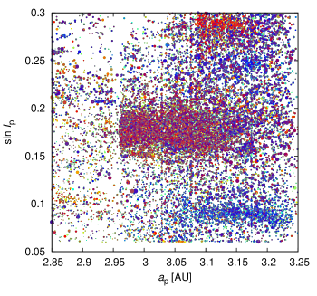
A rigorous comparison of observations versus simulations of asteroid families is a rather difficult task, especially when the observations look like Figure 1. Observed proper elements $a_{\rm p}$, $e_{\rm p}$, $\sin I_{\rm p}$, supplied by physical data (colour indices $a^{\star}$, $i-z$ in this case), show a complicated structure of the Eos family, halo, together with many neighbouring families, overlapping halos, and background asteroids, of course. The hierarchical clustering method alone (HCM, Zappalà et al. 1995) is then practically useless.

Family identification itself affects dynamical studies and vice versa. We would need the family to determine initial conditions. On the other hand, we would need a dynamical study to understand whereever family members could be. There are several well-known weaknesses of HCM, which were demonstrated e.g. in a ‘crime-scene’ Fig. 8 of Nesvorný et al. (2015). The HCM needs a free parameter, either the cutoff velocity $v_{\rm cut}$, or the quasi-random level ${\rm QRL}$. It is also unable to associate halos. Last but not least, the background is never precisely uniform what can be clearly seen at the edges of currently stable zones, close or inside gravitational resonances, or even in stable zones where the population was deteriorated by dynamical processes in the distant past (cf. Cybele region; Carruba et al. 2015).

On the other hand, synthetic families evolve in the course of simulation and loose their members, consequently we should use a variable $v_{\rm cut}$, but its optimal value is again generally unknown. No direct comparison is thus possible.

That is a motivation for our work. We describe a method suitable to study 3-dimensional shapes of asteroid families, taking into account all proper orbital elements, including possibly non-uniform background, and matching the size-frequency distribution at the same time. Our method still relies on a preliminary selection of observed asteroids according to their colours (or albedos) to suppress – but not fully exclude – interlopers. A comparison of the observed asteroids with an output of N-body simulation is performed by means of counting the bodies in proper-element ’boxes’, and a suitable $\chi^{2}$ metric. Because we are forced to select synthetic asteroids randomly (a Monte-Carlo approach), we can expect some stochasticity of the results.

We present an application to the Eos family (family identification number, FIN = 606), one of the most studied families to date, mentioned already by Hirayama (1918). Together with our previous works (Vokrouhlický et al., 2006; Brož and Morbidelli, 2013), this paper forms a long-term series focused on its long-term evolution. We use up-to-date catalogues of proper elements (Knežević and Milani, 2003), and brand new spin data (Hanuš et al., 2018).

Let us recall that the Eos family is of K taxonomic type, while the background is mostly C type. Mothé-Diniz et al. (2008) suggested either a partially differentiated parent body, with meteorite analogues CV, CO or R; or a undifferentiated one, with CK analogues. There was a discovery of a recent breakup of (6733) 1992 EF (Novaković and Tsirvoulis, 2014), belonging to the family core, what makes Eos even more interesting for space weathering studies, because we may see both old (1.3 Gyr) and young (4 Myr) surfaces.

Figure 1: Top panel: the proper semimajor axis $a_{\rm p}$ vs proper inclination $\sin I_{\rm p}$ for all asteroids in the broad surroundings of Eos family. The range of proper eccentricities is $e_{\rm p}\in(0.0;0.3)$. If they have colour data in the SDSS MOC4 catalogue (Parker et al., 2008), the colours correspond to indices $a^{\star}$, $i-z$ which are closely related to taxonomy, namely blue is close to C-complex taxonomy, red to S-complex, and magenta to K-type. The whole sample contains 18 471 asteroids. There are other prominent families visible: Hygeia (C-type, bottom-right), Veritas (C, next to Eos), Tirela (S, upper right), Telramund (S, below Eos); a close inspection would show 32 families in total! Bottom panel: the same plot for a typical outcome of N-body simulations, assuming a disruption of a parent body, ejection of fragments with some velocity field, and their long-term dynamical evolution due to gravitational perturbations, resonances, chaotic diffusion, the Yarkovsky effect, the YORP effect, etc. The two panels are not directly comparable.

2 Methods

Before we proceed with the description of the method, let us explain three problems we have to solve and describe the underlying dynamical model.

2.1 Problem 1: Selection of asteroids

In principle, we can select any subset of asteroids (e.g. by using SDSS colour data, or WISE albedo data) to decrease a contamination by interlopers, or an overlap with other families in the neighbourhood (Parker et al., 2008; Masiero et al., 2011); an approach also used in a multidomain HCM (Carruba et al., 2013). We can also simulate any subset at will, but we should definitely check surroundings where the bodies can be scattered to, because this may be a key constraint.

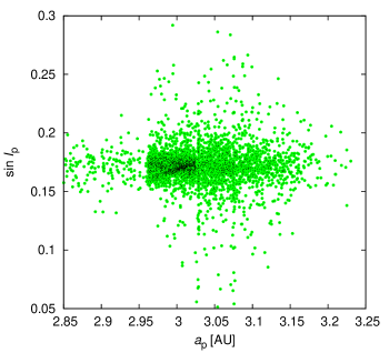
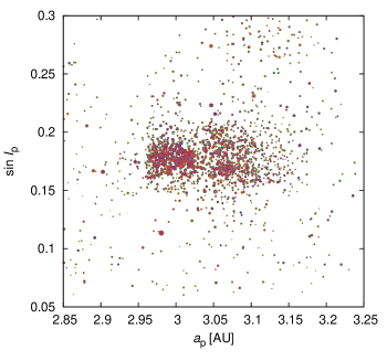
For Eos family, it is easy because of its distinct K taxonomic type which is defined for our purposes in terms of the SDSS colour indices $a^{*}\!\in(0.0,0.1)$, $i-z\in(-0.03,0.08)$, and the geometric albedo $p_{V}>0.07$ (if known in WISE or IRAS catalogues). If only colours are known, we select the asteroids according to them, and assume their $p_{V}=0.158$ which corresponds to the median value of Eos members. As a result, only 1/10^th of asteroids remain, but this is still sufficient (Figure 2). Practically all other families have disappeared, the background is much more uniform. The only exception may be some contamination from the Tirela family (seen as a concentration in the upper right corner of Fig. 2), arising from a photometric noise on S-type asteroids, and a gap at large $\sin I_{\rm p}>0.25$.

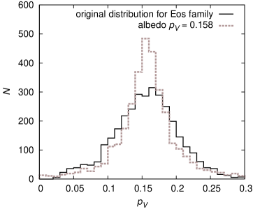
Regarding the homogeneity of albedos, the WISE data exhibit a wide distribution, and we should check whether it can be related to a heterogeneous parent body. The uncertainties $\sigma_{\!p}$ arise mainly from photon noise, and NEATM model systematics. In a statistical sense, even the single albedo value $\bar{p}_{V}=0.158$ would result in a relatively wide distribution because $\sigma_{\!p}$ values are relatively large, which is demonstrated in Figure 3, where we used the $\sigma$’s of individual measurements together with the (constant) $\bar{p}_{V}$ to randomly generate the new distribution of $p_{V}$’s. The Eos family thus seems homogeneous rather than heterogeneous.

Figure 2: K-type asteroids selected from Figure 1, with known colour indices $a^{*}\!\in(0.0;0.1)$, $i-z\in(-0.03;0.08)$. The visual geometric albedo had to be $p_{V}>0.07$ (or unknown). This subset is much more homogeneous and contains 1 991 asteroids. No other prominent families except Eos can be seen; the only exception may be some contamination by Tirela (upper right) due to inherent photometric noise. This subset seems already suitable for a comparison with N-body simulations.

Figure 3: The observed differential distribution of visual geometric albedos $p_{V}$ for the Eos family from the WISE catalogue (Masiero et al., 2011) (black solid), and for the same set of bodies with $p_{V}$ values assigned randomly, assuming a Gaussian distribution with a constant mean $\bar{p}_{V}=0.158$, and 1-$\sigma$ uncertainty declared in the catalogue (dashed gray). The widths of the two distributions are similar, so using the constant $\bar{p}_{V}$ (if unknown) is not a poor approximation.

2.2 Problem 2: Size-frequency distribution

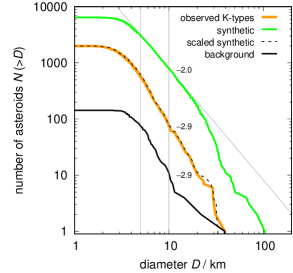
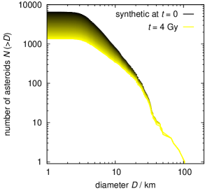
The size-frequency distributions (SFDs) should match for both the observed and synthetic populations, but the latter changes in the course of time (Figure 4). In order to compare apples with apples, we have to scale the SFD. In other words, we randomly select the same number of synthetic bodies (together with their orbits, of course) as the number of observed bodies, in each of prescribed size bins $(D,D+{\rm d}D)$. Let us emphasize we do not rely on the assumption of a constant SFD. To this point, it is definitively useful to start with a larger number of synthetic bodies, so that we still have more than observed at the end of simulation.

This random selection of synthetic asteroids to match the SFD of observed asteroids is needed at every single output time step of the simulation. Even multiple selections at one time step might be useful. This way, we would naturally account for an additional (and often neglected) uncertainty which arises from the fact we always choose the initial conditions from some underlying distributions (e.g. from a prescribed velocity field), but we cannot be absolutely sure that our single selection is not a lucky fluke.

Figure 4: Top panel: the cumulative size-frequency distribution (SFD) of the observed K-type asteroids (orange), the synthetic SFD at the beginning of N-body simulation (green), the scaled synthetic SFD constructed by a random selection of bodies so that it matches the observed one (dotted black; hard to distinguish from orange), and the background SFD (black). Bottom panel: an evolution of the synthetic SFD in the course of an N-body simulation, from time $t=0$ up to 4 Gyr, which is indicated by changing colours (black$\,\rightarrow\,$yellow). These changes (due to a dynamical decay) require scaling at every time step.

2.3 Problem 3: Non-uniform background

A background has to be accounted for otherwise it is essentially impossible to explain a lot of bodies far from the family. First, we need to find some observed background, not very far from the family; in our case, a suitable population seems to be at $\sin I_{\rm p}\in(0.06;0.12)$ and $(0.24;0.30)$. It has its own size-frequency distribution, and we should use the same SFD for the synthetic background. As a first approximation, we model the background as a random uniform distribution in the space of proper elements.

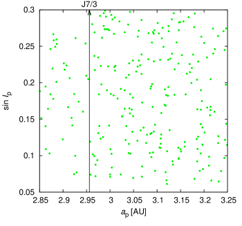
However, Murphy’s law for backgrounds states: The background is never uniform. Especially below and above the 7/3 mean-motion resonance with Jupiter we can expect a difference (see the example in Figure 5).

Again, there is a non-negligible stochasticity. We shall at least try a different random seed. The number density of background objects can be also treated as a free parameter. There is also a priori unknown systematic contamination by neighbouring families, but this is not necessarily present right ‘under’ the Eos family.

Figure 5: A synthetic background generated as a random uniform distribution in proper orbital elements $a_{\rm p},e_{\rm p},\sin I_{\rm p}$, with the same size-distribution as the observed background. In this example, the number densities below and above the 7/3 mean-motion resonance with Jupiter at 2.956 au are different (by a factor of 2), because this resonance separates two distinct zones of the main belt.

2.4 Dynamical model

Our dynamical model was described in detail in Brož et al. (2011). We briefly recall it contains a modified SWIFT integrator (Levison and Duncan, 1994; Laskar and Robutel, 2001), both the diurnal and seasonal Yarkovsky thermal effects (Vokrouhlický, 1998; Vokrouhlický and Farinella, 1999), which induce a semimajor axis drift ${\rm d}a/{\rm d}t$; all mean-motion and secular resonances, captures and corresponding drifts ${\rm d}e/{\rm d}t$, ${\rm d}I/{\rm d}t$, the YORP effect, changing the spin rate $\omega$ and the obliquity $\gamma$ (Čapek and Vokrouhlický, 2004), with the efficiency parameter $c_{\rm YORP}=0.33$ (Hanuš et al., 2011), simplified collisional reorientations by means of a prescribed time scale dependent on size $D$ (Farinella et al., 1998), random period changes due to mass shedding after reaching the critical spin rate $\omega_{\rm crit}$ (Pravec and Harris, 2000), and suitable digital filters for computations of mean and proper elements (Quinn et al., 1991; Šidlichovský and Nesvorný, 1996).

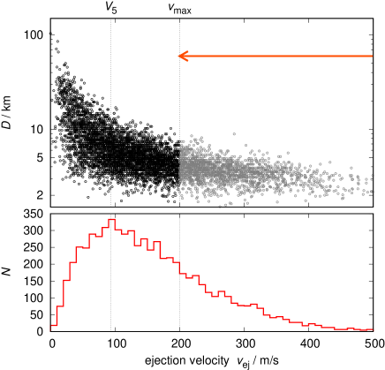
Initial conditions are kept as simple as possible. We assume an isotropic disruption, with the ejection velocity components Gaussian, with the dispersion proportional to $1/D$, and $V_{5}=93\,{\rm m}\,{\rm s}^{-1}$ for $D_{5}=5\,{\rm km}$, an estimate based on our previous work (Vokrouhlický et al., 2006). Consequently, the distrubution of the velocity magnitude $|\vec{v}_{\rm ej}|$ is Maxwellian (see Figure 6). We start with 6 545 synthetic bodies, with the SFD covering $D\in(1.5;100)\,{\rm km}$. Spins are also isotropic and periods uniform, $P\in(2;10)\,{\rm h}$.

Figure 6: Top panel: the dependence of the ejection velocity $v_{\rm ej}$ on the diameter $D$ for our synthetic bodies. The value $V_{5}=93\,{\rm m}\,{\rm s}^{-1}$ denotes the dispersion of velocity components for $D_{5}=5\,{\rm km}$ bodies. In specific cases (Sec. 3.2), we select only bodies with velocities smaller than some maximum value, $v_{\rm ej}<v_{\rm max}$. Bottom panel: the corresponding histogram of $v_{\rm ej}$.

The thermal parameters remain the same as in our previous works: the bulk density $\rho=2\,500\,{\rm kg}\,{\rm m}^{-3}$, the surface density $\rho=1\,500\,{\rm kg}\,{\rm m}^{-3}$, the conductivity $K=0.001\,{\rm W}\,{\rm m}^{-1}\,{\rm K}^{-1}$, the specific capacity $C=680\,{\rm J}\,{\rm kg}^{-1}$, the Bond albedo $A=0.1$, the infrared emissivity $\epsilon=0.9$. For simplicity, we assumed these parameters to be constants, although some of them may be size-dependent (as $K$ in Delbo et al. 2015), or temperature-dependent (Anderson et al., 1991).

The free parameters of our model are the maximum of velocity distribution $v_{\rm max}$ (Fig. 6), the true anomaly $f_{\rm imp}$, and the argument of pericentre $\omega_{\rm imp}$ at the time of impact, which are interrelated by means of the Gauss equations. We may be forced to tune also other osculating orbital elements of the parent body, but for the moment we take those of (221) Eos as the nominal case.

Among the fixed parameters is the bulk density $\rho$. Usually, the age scales linearly with $\rho$ due to the non-gravitational accelerations. Theoretically, if there are both gravitational and non-gravitational accelerations acting at the same time (e.g. Yarkovsky drift in $a$ and chaotic diffusion in $e$) we may be able to break this degeneracy. However, based on our previous experience, we do not expect this for Eos. Neighbouring Veritas may be more suitable for this approach, by the way. Alternatively, one can use collisional models which exhibit a different scaling with $\rho$ (cf. Sec. 4.1).

We integrate the equations of motion with the time step $\Delta t=91\,{\rm d}$, and the time span $4\,{\rm Gyr}$. The output time step after computations of mean elements, proper elements, and final running-window filter is $\Delta t_{\rm out}=10\,{\rm Myr}$.

2.5 Black-box method

We can eventually proceed with a so-called ‘black-box’ method (see Figure 7): (i) we choose 180 boxes with $\Delta a=0.0243\,{\rm au}$, $\Delta e=0.025$, $\Delta\sin I=0.240$ in our case aligned with the J7/3 and J9/4 resonances; (ii) count the numbers of observed asteroids located in these boxes; (iii) compute the observed incremental SFD globally, in the full domain; (iv) compute the background incremental SFD globally; (v) at every single output time step we compute the synthetic incremental SFD globally again (saving also lists of bodies in the respective size bins); (vi) for every single size bin $(D,D+{\rm d}D)$ we draw a synthetic background population of $N_{\rm bg}$ bodies from a random uniform distribution (in the whole range of $a_{\rm p},e_{\rm p},\sin I_{\rm p}$); if the volume where the background was selected differs from our volume of interest, we have to use a suitable factor, i.e. $fN_{\rm bg}$; (vii) we scale the synthetic SFD to the observed one by randomly choosing $N_{\rm obs}-fN_{\rm bg}$ bodies from the lists above; (viii) we count the numbers of all synthetic asteroids located in the boxes; (ix) finally, we compute the metric

$$\chi^{2}=\sum_{i=1}^{N_{\rm box}}{(N_{{\rm syn}\,i}-N_{{\rm obs}\,i})^{2}\over\sigma_{{\rm syn}\,i}^{2}+\sigma_{{\rm obs}\,i}^{2}}\,,$$ (1)

where the uncertainties are assumed Poisson-like, $\sigma=\sqrt{N}$. Using both $\sigma_{\rm obs}$ and $\sigma_{\rm syn}$ in the denominator prevents ‘extreme’ $\chi^{2}$ contributions in boxes where $N_{\rm obs}\to 0$. We shall keep in mind though the corresponding probability distribution of $\chi^{2}$ may be somewhat skewed. There is some freedom related to the box sizes (binning), but within the limits of meaningfulness (neither a single box nor zillions of boxes), the method should give statistically comparable results as we always analyse the same information.

Unlike traditional simplified methods fitting an envelope to $(a_{\rm p},H)$ or $(a_{\rm p},1/D)$, we shall obtain not only an upper limit for the age, but also a lower limit.

3 Results

Hereinafter, we discuss not only the best-fit model, but also several bad fits which are actually more important, because the ‘badness-of-fit’ assures a solid conclusion about the Eos family.

3.1 The nominal model

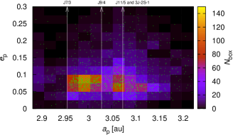
The nominal model is presented in Figure 7. We focus on the proper semimajor axis $a_{\rm p}$ vs proper eccentricity $e_{\rm p}$ distribution, having only one box in inclination $\sin I_{\rm p}$. The initial conditions (top left) are so different from the observations (bottom middle) it is almost hopeless to expect a good fit anytime in the future. However, at around $t=1.3\,{\rm Gyr}$ the situation suddenly changes (top middle); it is almost unbelievable that the synthetic family is so similar to the observations! The final state (top right) is again totally different. The $\chi^{2}$ reaches values as low as $N_{\rm box}$, so we may consider the best fit to be indeed reasonable. The age interval is $t=(1.3\pm 0.3)\,{\rm Gyr}$. Let us emphasize that the fit so good only because we carefully accounted for all three problems outlined in Section 2.

$t=0\,{\rm Myr}$	$t=1340\,{\rm Myr}$	$t=3980\,{\rm Myr}$
	observed	$\chi^{2}$ metric

Figure 7: The proper semimajor axis $a_{\rm p}$ vs proper eccentricity $e_{\rm p}$ for the nominal simulation scaled to the observed SFD (as described in the main text) (top row). Bodies are plotted as green dots. Colours correspond to the number of bodies in 180 boxes, outlined by $\Delta a=0.0234\,{\rm au}$, $\Delta e=0.025$. The range of inclinations is always $\sin I_{\rm p}\in(0.06;0.30)$. Positions of major mean-motion and 3-body resonances are also indicated (J7/3, J9/4, J11/5, and $3{\rm J}-2{\rm S}-1$). The $z_{1}$ secular resonance goes approximately from the lower-left corner to the upper-right. There are the initial conditions (left column), the best-fit at $t=1340\,{\rm Myr}$ (middle), the end of simulation (right); as well as the observations (bottom middle), and the respective $\chi^{2}$ metric compared to the actual number of boxes $N_{\rm box}$ (bottom right). The correspondence between the best-fit and the observations is surprisingly good, with $\chi^{2}=141$, $N_{\rm box}=134$ (not all boxes are populated), and $\chi^{2}\simeq N_{\rm box}$. The 1-$\sigma$, 2-$\sigma$ and 3-$\sigma$ levels (dotted lines) and the inferred 3-$\sigma$ uncertainty of the age (yellow strip) are indicated too.

3.2 Bad fit 1: Ejection velocity tail

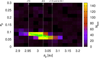
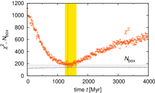
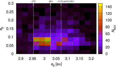
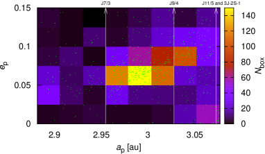
Because our sample is 3 times larger than the observed sample, we can easily resample our synthetic bodies without actually computing the N-body simulation anew, e.g. selecting only those with low ejection velocity $v_{\rm ej}<200\,{\rm m}\,{\rm s}^{-1}$. Consequently, all bodies are initially located above the J7/3 resonance, and below the J11/5.

Using the same post-processing as above we arrived at Figure 8. It is clear that the ‘best fit’ is actually a bad fit compared to the nominal model. The notable differences are below the J7/3 resonance, and above the J11/5 where the numbers of bodies are never sufficient to match the observations (cf. Fig. 7, bottom middle).

It is worth to note there is a small family just below the J7/3 resonance, namely (36256) 1999 XT₁₇ (FIN 629). Tsirvoulis et al. (2018) discovered a link to Eos by analysing the overall V-shape in the semimajor axis $a_{\rm p}$ vs the absolute magnitude $H$ diagram. It seems aligned with the original velocity field of the Eos family — it has the same $\sin I_{\rm p}$ as the family core, but slightly larger $e_{\rm p}\simeq 0.1$, because of the ‘ellipse’ in $(a_{\rm p},e_{\rm p})$ visible in Fig. 7 (top left). We thus conclude, (36256) family is actually a remnant of the original velocity field.

If this is true, it may further contribute to the contamination of the ‘pristine zone’ between the J7/3 and J5/2 resonances, apart from low-probability crossings of the former resonance. This region was analysed by Tsirvoulis et al. (2018), where authors carefully subtracted the contribution of all families (including Eos), extracted the SFD of remaining background asteroids and computed the slope of the primordial (post-accretion) SFD.

$t=1430\,{\rm Myr}$

Figure 8: Bad fit 1: the proper semimajor axis $a_{\rm p}$ vs proper eccentricity $e_{\rm p}$ (top panel), and the temporal evolution of $\chi^{2}$ (bottom panel) for a subset of bodies with the ejection velocities $v_{\rm ej}<200\,{\rm m}\,{\rm s}^{-1}$, i.e. without the tail of the distribution. Initially, all bodies were located above the J7/3 resonance. Observations were shown in Fig. 7 (bottom middle). The ‘best-fit’ at $t=1430\,{\rm Myr}$, with $\chi^{2}=197$, $N_{\rm box}=134$, is much worse than the nominal case. The number of bodies below the J7/3 resonance is too low. Consequently, the velocity tail is needed to get a better fit.

3.3 Bad fit 2: Parent body inclination

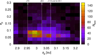
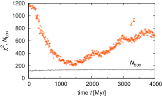
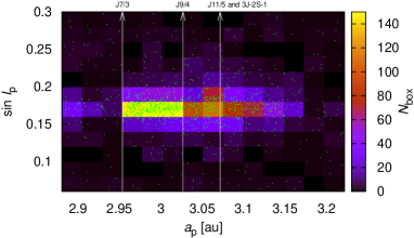
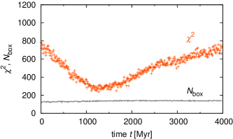
If we look on contrary on the proper semimajor axis $a_{\rm p}$ vs proper inclination $\sin I_{\rm p}$ distribution (Figure 9) there is a problem with the nominal model. Inclinations are all the time too low (and the $\chi^{2}$ too high compared to $N_{\rm box}$). This would affect a 3-dimensional fit too, of course.

Nevertheless, it seems sufficient to adjust the inclination by approximately $0.005\,{\rm rad}$ to get a significantly better fit, $\chi^{2}$ decreased from 238 down to 181. This seems still too high wrt. 130, but this approach is possibly too simplified, because we only shifted the output data. In reality, the resonances (in particular the $z_{1}$) do not shift at all, they are determined by the positions of giant planets, and we should perform the N-body integration anew to obtain a correct $(a_{\rm p},\sin I_{\rm p})$ distribution.

$t=1270\,{\rm Myr}$

Figure 9: Bad fit 2: the proper semimajor axis $a_{\rm p}$ vs proper inclination $\sin I_{\rm p}$ for the synthetic population (top panel), and the temporal evolution of $\chi^{2}$ (bottom panel). The boxes are consequently different, $\Delta a=0.0243\,{\rm au}$, $\Delta\sin I=0.02$, $e_{\rm p}\in(0.0;0.3)$, so is the resulting ‘best-fit’ value $\chi^{2}=238$, $N_{\rm box}=130$. The parent body would have to be shifted in inclination by approximately $0.005\,{\rm rad}$ to get a better fit.

3.4 Bad fit 3: True anomaly $f_{\rm imp}<120^{\circ}$

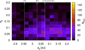
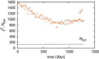
To demonstrate the sensitivity of our ‘black-box’ method with respect to the impact parameters, we present an alternative N-body simulation which started with the true anomaly $f_{\rm imp}=0^{\circ}$. The orientation of the ellipse is then the opposite and there is practically no chance for a good fit (see Figure 10).

All the time, there is a serious mismatch within the family core, it is impossible explain the observed bodies in the boxes with $a_{\rm p}\simeq 2.97\,{\rm au}$, and $e_{\rm p}\simeq 0.08$. Generally, it is surprising that even $1.3\,{\rm Gyr}$ after the impact, there are clear traces of the original velocity field! As already reported in Brož and Morbidelli (2013), the ‘true’ true anomaly should be $f>120^{\circ}$. Another example of such traces (in inclination) is Koronis family (Carruba et al., 2016).

$t=1280\,{\rm Myr}$

Figure 10: Bad fit 3: a detail of the proper semimajor axis $a_{\rm p}$ vs proper eccentricity $e_{\rm p}$ (top panel), and the temporal evolution of $\chi^{2}$ (bottom panel) for the simulation with the true anomaly at the time of impact $f_{\rm imp}=0^{\circ}$, and the argument of perihelion $\omega_{\rm imp}=30^{\circ}$. The ‘best-fit’ $\chi^{2}=711$ is so high compared to $N_{\rm box}=124$ that the simulation was not computed up to $4000\,{\rm Myr}$. The value has to be $f\gtrsim 120^{\circ}$ to get a better fit.

4 Conclusions

Let us conclude, it is important to use a suitable selection of asteroids, match the size-frequency distributions, and account for the background population, when comparing N-body simulations with observations. To this point, we presented and tested a simple method how to compare a 3-dimensional distribution of proper elements.

For the Eos family, it is possible to explain its shape in the $(a_{\rm p},e_{\rm p},\sin I_{\rm p})$ space and estimate the age at the same time, but this estimate still scales with the bulk density $\rho$, because most of the perturbations are non-gravitational (including all systematic drifts ${\rm d}a/{\rm d}t$, ${\rm d}e/{\rm d}t$, ${\rm d}I/{\rm d}t$).

While we believe our model includes the key contributions, no dynamical model is complete. For example, we miss inner planets, gravitational perturbations by large asteroids, or short-term spin axis evolution due to gravitational (solar) torques. Initial condition might be also too simple. In particular, the velocity field might have been non-isotropic even though in catastrophic disruptions (like Eos) we rather expect a high degree of isotropy (Ševeček et al., 2017). Generally, it is better to keep both as simple as possible to have the lowest possible number of free parameters.

Let us finally compare our nominal best-fit model to another two distributions (size and spin) and the respective models (collisional and rotational).

4.1 Collisional evolution

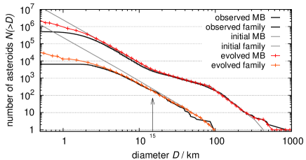
In a Monte-Carlo collisional model, size-frequency distributions are evolved due to fragmentation and reaccumulation. We assume two populations: the main belt, and the Eos family. Their physical properties are summarized by the scaling law $Q^{\star}_{\rm D}(r)$, for which we assume parameters of basalt at $5\,{\rm km}\,{\rm s}^{-1}$ from Benz and Asphaug (1999). To compute the actual evolution, we use the Boulder code by Morbidelli et al. (2009). Parametric relations in the Boulder code, which are needed to compute the fragment distributions, are derived from SPH simulations of Durda et al. (2007).

We assume the initial SFD of the main belt relatively similar to the currently observed SFD, because we focus on the already stable solar system, with the fixed intrinsic impact probability $P_{\rm imp}=3.1\times 10^{-18}\,{\rm km}^{-2}\,{\rm yr}^{-1}$ and the mean velocity $v_{\rm imp}=5.28\,{\rm km}\,{\rm s}^{-1}$. The initial SFD of the Eos family has the same slope as the observed SFD in the range $D\in(15;50)\,{\rm km}$, and it is prolonged down to $D_{\rm min}=0.005\,{\rm km}$. We also account for the size-dependent dynamical decay due to the Yarkovsky effect, with $N(t+\Delta t)=N(t)\exp(-\Delta t/\tau)$, where the time scale $\tau(D)$ is taken from Bottke et al. (2005).

The resulting collisional evolution is shown in Figure 11. The observed knee at $D\simeq 15\,{\rm km}$ is very important, because it usually arises from a collisional grinding. If we start with the constant slope from above, we can match the observed SFD at about $1.3\,{\rm Gyr}$ which is in accord with the dynamics.

It is worth to note the scaling of the age with the bulk density $\rho$ is different from dynamics, which in principle allows to resolve the problem. However, the collisional model is sensitive to the initial conditions and using a steeper SFD would result in longer age. In other words, everything is based on the simple assumption of the constant slope. It would be useful to base the initial conditions on a specific SPH model for the Eos family, with the parent body size reaching up to 380 km (according to an extrapolation of Durda et al. 2007 results).

$t=1300\,{\rm Myr}$

Figure 11: The cumulative size-frequency distributions computed by our Monte-Carlo collisional model of the two populations: the main belt (red), the Eos family (orange), together with the respective initial conditions (gray), and observations (black). At the time around $t=1300\,{\rm Myr}$ the correspondence is good, except the tail below $D\lesssim 2\,{\rm km}$ where an observational incompleteness makes the SFD’s shallow. In particular, we successfully fit the knee of the family at $D\simeq 15\,{\rm km}$.

4.2 Spin distribution

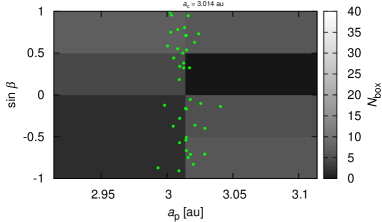
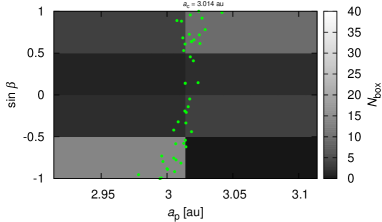
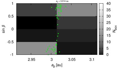
At the same time, it is worth to check the observed distribution of pole latitudes $\beta$, reported in Hanuš et al. (2018). Our dynamical model evolves the spin $(\omega,\gamma)$, which affects the Yarkovsky drift rate ${\rm d}a/{\rm d}t$, but we do not account for spin-orbital resonances (so we would not explain a clustering in the Koronis family; Slivan 2002). Nevertheless, if we use the current model for Eos, with the same post-processing, but focus on $(a_{\rm p},\sin\beta)$ boxes instead, we obtain the results summarized in Figure 12.

We start from an isotropic distribution of spins, which means isotropic also in $\sin\beta$. After about $1.3\,{\rm Gyr}$, it is possible to fit both the asymmetry of the distribution with respect to $a_{\rm c}=3.014\,{\rm au}$, and the substantially lower number of bodies at mid-latitudes $|\sin\beta\,|<0.5$. There are two systematics still present in our analysis, as we account neither for the observational selection bias, nor for the bias of the inversion method, but they should not overturn our conclusions.

Unfortunately, the uncertainty is larger than in the nominal model, because the number of bodies with known latitudes is limited, namely 46 within the family core. As a solution, we may use the distribution of $|\beta|$ of Cibulková et al. (2016) which is available for many more asteroids, but we would need to determine the ’point-spread function’, describing a relation between input $|\beta|$ and output $|\beta|$ for this (approximate) method, which smears the distribution substantially. Their sample also contains a lot of bodies smaller than we had in the previous simulations, so we would have to compute everything again. This is postponed as a future work.

$t=0\,{\rm Myr}$

$t=1260\,{\rm Myr}$

observed

Figure 12: The proper semimajor axis $a_{\rm p}$ vs the sine of pole latitude $\sin\beta$ for the initial synthetic population (top panel), the evolved synthetic population (middle), and the observed population of 46 bodies (bottom). The individual bodies are shown as green dots, while their numbers in 8 boxes are indicated by the gray scale. The simulation started from initially isotropic random distribution, i.e. isotropic in $\sin\beta$. The synthetic SFD was again scaled to the observed one. We account neither for the observational selection bias, nor for the bias of the inversion method. Nevertheless, it is possible to fit both the asymmetry of the distribution with respect to $a_{\rm c}=3.014\,{\rm au}$, and the substantially lower number of bodies at mid-latitudes $|\sin\beta\,|<0.5$.

References

- Anderson et al. (1991) Anderson, O.L., Isaak, D.L., Oda, H., 1991. Thermoelastic parameters for six minerals at high temperature. J. Geophys. Res. 96, 18037. doi:10.1029/91JB01579.
- Benz and Asphaug (1999) Benz, W., Asphaug, E., 1999. Catastrophic Disruptions Revisited. Icarus 142, 5–20. doi:10.1006/icar.1999.6204, arXiv:arXiv:astro-ph/9907117.
- Bottke et al. (2005) Bottke, W.F., Durda, D.D., Nesvorný, D., Jedicke, R., Morbidelli, A., Vokrouhlický, D., Levison, H.F., 2005. Linking the collisional history of the main asteroid belt to its dynamical excitation and depletion. Icarus 179, 63–94. doi:10.1016/j.icarus.2005.05.017.
- Brož and Morbidelli (2013) Brož, M., Morbidelli, A., 2013. The Eos family halo. Icarus 223, 844–849. doi:10.1016/j.icarus.2013.02.002, arXiv:1302.1447.
- Brož et al. (2011) Brož, M., Vokrouhlický, D., Morbidelli, A., Nesvorný, D., Bottke, W.F., 2011. Did the Hilda collisional family form during the late heavy bombardment? Mon. Not. R. Astron. Soc. 414, 2716–2727. doi:10.1111/j.1365-2966.2011.18587.x, arXiv:1109.1114.
- Čapek and Vokrouhlický (2004) Čapek, D., Vokrouhlický, D., 2004. The YORP effect with finite thermal conductivity. Icarus 172, 526–536. doi:10.1016/j.icarus.2004.07.003.
- Carruba et al. (2013) Carruba, V., Domingos, R.C., Nesvorný, D., Roig, F., Huaman, M.E., Souami, D., 2013. A multidomain approach to asteroid families’ identification. Mon. Not. R. Astron. Soc. 433, 2075–2096. doi:10.1093/mnras/stt884, arXiv:1305.4847.
- Carruba et al. (2016) Carruba, V., Nesvorný, D., Aljbaae, S., 2016. Characterizing the original ejection velocity field of the Koronis family. Icarus 271, 57–66. doi:10.1016/j.icarus.2016.01.006, arXiv:1602.04491.
- Carruba et al. (2015) Carruba, V., Nesvorný, D., Aljbaae, S., Huaman, M.E., 2015. Dynamical evolution of the Cybele asteroids. Mon. Not. R. Astron. Soc. 451, 244–256. doi:10.1093/mnras/stv997, arXiv:1505.03745.
- Cibulková et al. (2016) Cibulková, H., Ďurech, J., Vokrouhlický, D., Kaasalainen, M., Oszkiewicz, D.A., 2016. Distribution of spin-axes longitudes and shape elongations of main-belt asteroids. Astron. Astrophys. 596, A57. doi:10.1051/0004-6361/201629192, arXiv:1610.02790.
- Delbo et al. (2015) Delbo, M., Mueller, M., Emery, J.P., Rozitis, B., Capria, M.T., 2015. Asteroid Thermophysical Modeling. pp. 107–128.
- Durda et al. (2007) Durda, D.D., Bottke, W.F., Nesvorný, D., Enke, B.L., Merline, W.J., Asphaug, E., Richardson, D.C., 2007. Size-frequency distributions of fragments from SPH/ N-body simulations of asteroid impacts: Comparison with observed asteroid families. Icarus 186, 498–516. doi:10.1016/j.icarus.2006.09.013.
- Farinella et al. (1998) Farinella, P., Vokrouhlický, D., Hartmann, W.K., 1998. Meteorite Delivery via Yarkovsky Orbital Drift. Icarus 132, 378–387. doi:10.1006/icar.1997.5872.
- Hanuš et al. (2018) Hanuš, J., Delbo’, M., Alí-Lagoa, V., Bolin, B., Jedicke, R., Ďurech, J., Cibulková, H., Pravec, P., Kušnirák, P., Behrend, R., Marchis, F., Antonini, P., Arnold, L., Audejean, M., Bachschmidt, M., Bernasconi, L., Brunetto, L., Casulli, S., Dymock, R., Esseiva, N., Esteban, M., Gerteis, O., de Groot, H., Gully, H., Hamanowa, H., Hamanowa, H., Krafft, P., Lehký, M., Manzini, F., Michelet, J., Morelle, E., Oey, J., Pilcher, F., Reignier, F., Roy, R., Salom, P.A., Warner, B.D., 2018. Spin states of asteroids in the Eos collisional family. Icarus 299, 84–96. doi:10.1016/j.icarus.2017.07.007, arXiv:1707.05507.
- Hanuš et al. (2011) Hanuš, J., Ďurech, J., Brož, M., Warner, B.D., Pilcher, F., Stephens, R., Oey, J., Bernasconi, L., Casulli, S., Behrend, R., Polishook, D., Henych, T., Lehký, M., Yoshida, F., Ito, T., 2011. A study of asteroid pole-latitude distribution based on an extended set of shape models derived by the lightcurve inversion method. Astron. Astrophys. 530, A134. doi:10.1051/0004-6361/201116738, arXiv:1104.4114.
- Hirayama (1918) Hirayama, K., 1918. Groups of asteroids probably of common origin. Astron. J. 31, 185–188. doi:10.1086/104299.
- Knežević and Milani (2003) Knežević, Z., Milani, A., 2003. Proper element catalogs and asteroid families. Astron. Astrophys. 403, 1165–1173. doi:10.1051/0004-6361:20030475.
- Laskar and Robutel (2001) Laskar, J., Robutel, P., 2001. High order symplectic integrators for perturbed Hamiltonian systems. Celestial Mechanics and Dynamical Astronomy 80, 39–62. arXiv:arXiv:astro-ph/0005074.
- Levison and Duncan (1994) Levison, H.F., Duncan, M.J., 1994. The long-term dynamical behavior of short-period comets. Icarus 108, 18–36. doi:10.1006/icar.1994.1039.
- Masiero et al. (2011) Masiero, J.R., Mainzer, A.K., Grav, T., Bauer, J.M., Cutri, R.M., Dailey, J., Eisenhardt, P.R.M., McMillan, R.S., Spahr, T.B., Skrutskie, M.F., Tholen, D., Walker, R.G., Wright, E.L., DeBaun, E., Elsbury, D., Gautier, IV, T., Gomillion, S., Wilkins, A., 2011. Main Belt Asteroids with WISE/NEOWISE. I. Preliminary Albedos and Diameters. Astrophys. J. 741, 68. doi:10.1088/0004-637X/741/2/68, arXiv:1109.4096.
- Morbidelli et al. (2009) Morbidelli, A., Bottke, W.F., Nesvorný, D., Levison, H.F., 2009. Asteroids were born big. Icarus 204, 558–573. doi:10.1016/j.icarus.2009.07.011, arXiv:0907.2512.
- Mothé-Diniz et al. (2008) Mothé-Diniz, T., Carvano, J.M., Bus, S.J., Duffard, R., Burbine, T.H., 2008. Mineralogical analysis of the Eos family from near-infrared spectra. Icarus 195, 277–294. doi:10.1016/j.icarus.2007.12.005.
- Nesvorný et al. (2015) Nesvorný, D., Brož, M., Carruba, V., 2015. Identification and Dynamical Properties of Asteroid Families. pp. 297–321.
- Novaković and Tsirvoulis (2014) Novaković, B., Tsirvoulis, G., 2014. Recent disruption of an asteroid from the Eos family, in: Muinonen, K., Penttilä, A., Granvik, M., Virkki, A., Fedorets, G., Wilkman, O., Kohout, T. (Eds.), Asteroids, Comets, Meteors 2014.
- Parker et al. (2008) Parker, A., Ivezić, Ž., Jurić, M., Lupton, R., Sekora, M.D., Kowalski, A., 2008. The size distributions of asteroid families in the SDSS Moving Object Catalog 4. Icarus 198, 138–155. doi:10.1016/j.icarus.2008.07.002, arXiv:0807.3762.
- Pravec and Harris (2000) Pravec, P., Harris, A.W., 2000. Fast and Slow Rotation of Asteroids. Icarus 148, 12–20. doi:10.1006/icar.2000.6482.
- Quinn et al. (1991) Quinn, T.R., Tremaine, S., Duncan, M., 1991. A three million year integration of the earth’s orbit. Astron. J. 101, 2287–2305. doi:10.1086/115850.
- Ševeček et al. (2017) Ševeček, P., Brož, M., Nesvorný, D., Enke, B., Durda, D., Walsh, K., Richardson, D.C., 2017. SPH/N-Body simulations of small ( km) asteroidal breakups and improved parametric relations for Monte-Carlo collisional models. Icarus 296, 239–256. doi:10.1016/j.icarus.2017.06.021.
- Šidlichovský and Nesvorný (1996) Šidlichovský, M., Nesvorný, D., 1996. Frequency modified Fourier transform and its applications to asteroids. Celestial Mechanics and Dynamical Astronomy 65, 137–148. doi:10.1007/BF00048443.
- Slivan (2002) Slivan, S.M., 2002. Spin vector alignment of Koronis family asteroids. Nature 419, 49–51. doi:10.1038/nature00993.
- Tsirvoulis et al. (2018) Tsirvoulis, G., Morbidelli, A., Delbo’, M., Tsiganis, K., 2018. Reconstructing the size distribution of the primordial Main Belt. Icarus 304, 14–23.
- Vokrouhlický (1998) Vokrouhlický, D., 1998. Diurnal Yarkovsky effect as a source of mobility of meter-sized asteroidal fragments. I. Linear theory. Astron. Astrophys. 335, 1093–1100.
- Vokrouhlický et al. (2006) Vokrouhlický, D., Brož, M., Morbidelli, A., Bottke, W.F., Nesvorný, D., Lazzaro, D., Rivkin, A.S., 2006. Yarkovsky footprints in the Eos family. Icarus 182, 92–117. doi:10.1016/j.icarus.2005.12.011.
- Vokrouhlický and Farinella (1999) Vokrouhlický, D., Farinella, P., 1999. The Yarkovsky Seasonal Effect on Asteroidal Fragments: A Nonlinearized Theory for Spherical Bodies. Astron. J. 118, 3049–3060. doi:10.1086/301138.
- Zappalà et al. (1995) Zappalà, V., Bendjoya, P., Cellino, A., Farinella, P., Froeschlé, C., 1995. Asteroid families: Search of a 12,487-asteroid sample using two different clustering techniques. Icarus 116, 291–314. doi:10.1006/icar.1995.1127.