Isotropy Groups and Kinematic Orbits

for 1 and 2-$d$ $N$-Body Problems

Edward Anderson^∗

Mitchell and Littlejohn showed that isotropy groups and orbits for $N$-body problems attain a sense of genericity for $N=5$. The author recently showed that the arbitrary-$d$ generalization of this 3-$d$ result is that genericity in this sense occurs for $N=d+2$. The author also showed that a second sense of genericity – now order-theoretic rather than a matter of counting – occurs for $N=2d+1$, excepting $d=3$, for which it is not 7 but 8. Applications of this work include 1) that some of the increase in complexity in passing from 3 to 4 and 5 body problems in 3-$d$ is already present in the more-well known setting of passing from intervals to triangles and then to quadrilaterals in 2-$d$. 2) That not $(d,N)=(3,6)$ but (4, 6) is a natural theoretical successor of (3, 5). 3) Such consideration isotropy groups and orbits is moreover a model for a larger case of interest, namely that of GR’s reduced configuration spaces. The current Article presents the lower-$d$ cases explicitly: 0, 1 and 2-$d$, including also the topological and geometrical form of the corresponding isotropy groups and orbits.

PACS: 04.20.Cv , 02.40.Yy , 02.70.Ns .

Physics keywords: $N$-Body Problem, Configuration Spaces, Background Independence, Topological and Geometrical Methods in Theoretical Physics.

Mathematics keywords: Shape Theory, Applied Geometry, Topology and Linear Algebra.

^∗ Dr.E.Anderson.Maths.Physics *at* protonmail.com

1 Introduction

The $N$-Body Problem rapidly develops technical complexity with increasing $N$ [13, 14, 15, 30, 33, 34, 21, 19, 41, 51, 69]. Even $N=3$ is considered to be hard, $N=4$ harder, and $N=5$ the limit of current-era detailed study for specific $N$. This is moreover with reference to 3-$d$; 1- and 2-$d$ exhibit a number of more systematic features [4, 10, 13, 14, 22, 36, 69] Finally, we recently noted [69] that many qualitative features depend on the combination $(d,\,N)$ rather than just on $d$, placing further interest in lower-$d$ specific examples (the current Article) and higher-$d$ ones (for subsequent study: see the Conclusion).

Our study is at the level of configuration space, more specifically of shape space and relational space (alias shape-and-scale space). These are outlined in Sec 2, and constitute an elementary part of Shape Theory [22, 23, 31, 35, 36, 43, 46, 49, 53, 50, 59, 60, 61, 62, 63, 64, 65, 66]. These structures arise moreover as part of Background Independence [5, 6, 7, 8, 9, 16, 25, 44, 56, 57, 62, 67, 68]; the well-known Problem of Time [9, 8, 26, 27, 47, 52, 56, 62] can moreover be viewed as difficulties arising in attempting to implement Background Independence.

The current Article considers more specifically isotropy groups and kinematic orbits in the shapes-and-scales case of quotienting out by the Euclidean group. We approach this with various uses of Linear Algebra and one of Differential Geometry in Sec 3, and explicit examples in Sec 2. By further material in Sec 2, this readily reduces to just quotienting out rotations by passing to centre of mass frame and applying the Jacobi map. We consider, firstly, Mitchell and Littlejohn’s criterion [41] of minimal point-or-particle number $N$ required to distinctly realizing a full count of isotropy subgroups. Secondly, which minimal $N$ is required for these isotropy subgroups to form the generic bounded lattice of subgroups [69]. These are ‘C’ and ‘O’ genericity criteria respectively, standing for ‘counting’ and ‘order’. We concentrate on the 0-, 1- and 2-$d$ cases, [30, 34, 41, 69] having already detailed 3-$d$, working as far up as the first counting-generic and order-generic $N$. Key underlying results are, firstly, that C-genericity occurs for

$$N=d+2$$ (1)

rather than just specifically for $(d,\,N)=(3,\,5)$. Secondly, that a bound on O-genericity occurs for

$$N=2\,d+1$$ (2)

except for $d=3$ itself, for which a Lie group accidental relation pushes it up to 8. This means that the well-studied quadrilaterals (2, 4) are a model arena for (3, 5), and that the pentagons (2, 5) are in some ways a model arena for the O-generic (3, 8). The well-known progression from intervals (2, 2) to triangles (2, 3) to guadrilaterals is moreover a model for some features of the key progression in complexity in passing from 3- to 4- to 5-Body Problems in 3-$d$.

Such consideration isotropy groups and orbits is moreover of further interest as a model for a larger case of interest, namely that of GR’s reduced configuration spaces [8, 11, 12, 32, 45], as well as of some specifically global [62] aspects of Background Independence and the Problem of Time.

In the current Article, we provide 0, 1 and 2-$d$ counterparts of [41]’s analysis in support of [69]’s point that their analysis is counting-generic for . Thus (0, 2), (1, 3) and (2, 4) are considered here, as well as the partial realizations for smaller $N$’s than these in each case. We conclude with an outline of pointers to further research directions in Sec 8; see also [69, 71] for further details.

2 Some configuration spaces for $N$-Body Problem

The carrier space $\mbox{\boldmath${\mathfrak{M}}$}^{d}$, alias absolute space in the physical context is an at least provisional model for the structure of space.

Constellation space (reviewed in [49]) is the product of $N$ copies of carrier space,

$$\mbox{\Large$\mathfrak{q}$}(\mbox{\boldmath${\mathfrak{M}}$}^{d},\,N)\mbox{ }=\mbox{ }\mbox{\Large$\times$}_{I=1}^{N}\mbox{\boldmath${\mathfrak{M}}$}^{N}$$ (3)

modelling $N$ points on ${\mathfrak{M}}$, or, if these points are materially realized, $N$ particles (classical, nonrelativistic).

In the current Article, we consider the most common setting for the $N$-Body Problem,

$$\mbox{\boldmath${\mathfrak{M}}$}=\mathbb{R}^{n}\mbox{ },$$ (4)

by which

$$\mbox{\Large$\mathfrak{q}$}(d,\,N):=\mbox{\Large$\mathfrak{q}$}(\mathbb{R}^{d},\,N)\mbox{ }=\mbox{ }\mbox{\Large$\times$}_{I=1}^{N}\mathbb{R}^{d}\mbox{ }=\mbox{ }\mathbb{R}^{N\,d}\mbox{ }.$$ (5)

We further narrow this down to $d=0,1,2$, [41] having already carried out the analysis in question for the most commonly considered $N$-body setting of all, $\mathbb{R}^{3}=3$.

Relative space (see [49, 63, 69])is the quotient of constellation space by the group of translations,

$$Tr(d)=\mathbb{R}^{d}\mbox{ },$$ (6)

yielding

$$\mbox{\Large$\mathfrak{r}$}(d,\,N)\mbox{ }:=\mbox{ }\frac{\mbox{\Large$\mathfrak{q}$}(\mathbb{R}^{d},\,N)}{Tr(d)}\mbox{ }=\mbox{ }\frac{\mathbb{R}^{d\,N}}{\mathbb{R}^{d}}\mbox{ }=\mbox{ }\mathbb{R}^{d\,n}\mbox{ }.$$ (7)

This last equation holds both topologically and metrically, as is most easily seen [69] by passing to mass-weighted relative Jacobi coordinates [24]. These maintain form of kinetic metric but with one object less; this can be viewed as result of diagonalizing the relative separations.

$$n:=N-1$$ (8)

is the number of independent relative separations.

Preshape space [22, 36, 63] is the quotient of constellation space by the dilatational group comprised of translations and dilations,

$$Dilatat(d)\mbox{ }=\mbox{ }Tr(d)\rtimes Dil\mbox{ }=\mbox{ }\mathbb{R}^{n}\rtimes\mathbb{R}_{+}\mbox{ },$$ (9)

where $\rtimes$ denotes semidirect product of groups [40]. This yields

$$\mbox{\Large$\mathfrak{p}$}(d,\,N)\mbox{ }:=\mbox{ }\frac{\mbox{\Large$\mathfrak{q}$}(d,\,N)}{Dilatat(d)}\mbox{ }=\mbox{ }\frac{\mathbb{R}^{N\,d}}{\mathbb{R}^{n}\rtimes\mathbb{R}_{+}}\mbox{ }=\mbox{ }\frac{\mathbb{R}^{d\,N}}{\mathbb{R}_{+}}\mbox{ }=\mbox{ }\mathbb{S}^{n\,d-1}\mbox{ },$$ (10)

this last result being Kendall’s preshape sphere, at both the topological and metric levels of structure.

Shape space [22, 23, 36] is the quotient of constellation space by the similarity group comprised of translations, dilations and rotations,

$$Sim(d)\mbox{ }=\mbox{ }Tr(d)\rtimes(Dil\times SO(d))\mbox{ }=\mbox{ }\mathbb{R}^{n}\rtimes(\mathbb{R}_{+}\times SO(d))\mbox{ },$$ (11)

where $\times$ denotes direct product of groups [40]. This yields

$$\mbox{\Large$\mathfrak{s}$}(d,\,N)\mbox{ }:=\mbox{ }\frac{\mbox{\Large$\mathfrak{q}$}(d,\,N)}{Sim(d)}\mbox{ }=\mbox{ }\frac{\mathbb{R}^{N\,d}}{\mathbb{R}^{n}\rtimes(\mathbb{R}_{+}\times SO(d))}\mbox{ }=\mbox{ }\frac{\mathbb{R}^{n\,d}}{\mathbb{R}_{+}\times\times SO(d)}\mbox{ }=\mbox{ }\frac{\mathbb{S}^{n\,d-1}}{SO(d)}\mbox{ }.$$ (12)

In 1-$d$, there are no continuous rotations, so shape space coincides with preshape space

$$\mbox{\Large$\mathfrak{s}$}(1,\,N)=\mbox{\Large$\mathfrak{p}$}(1,\,N)=\mathbb{S}^{n-1}\mbox{ }.$$ (13)

In 2-$d$,

$$SO(2)=U(1)$$ (14)

and e.g. [70] the generalized Hopf map [18] gives that

$$\mbox{\Large$\mathfrak{s}$}(2,\,N)\mbox{ }=\mbox{ }\frac{\mathbb{S}^{2\,n-1}}{U(1)}\mbox{ }=\mbox{ }\mathbb{CP}^{n-1}\mbox{ }:$$ (15)

complex-projective spaces of $N$-a-gons [22, 36, 50] as equipped with the standard Fubini–Study metric [18].

Exceptionally for $N=3$, the Hopf map itself gives

$$\mbox{\Large$\mathfrak{s}$}(2,\,3)\mbox{ }=\mbox{ }\mathbb{CP}^{1}\mbox{ }=\mbox{ }\mathbb{S}^{2}$$ (16)

– the sphere of triangles in 2-$d$ [22, 23, 36, 65] –with this case’s Fubini–Study metric collapsing to the standard spherical metric.

Relational space alias scaled shape space is the quotient of constellation space by the Euclidean group of translations and rotations,

$$Eucl(d)\mbox{ }=\mbox{ }Tr(d)\rtimes(Dil\times SO(d))\mbox{ }=\mbox{ }\mathbb{R}^{n}\rtimes\times SO(d)\mbox{ }.$$ (17)

This yields

$$\mbox{\boldmath$\mathfrak{R}$}(d,\,N)\mbox{ }:=\mbox{ }\frac{\mbox{\Large$\mathfrak{q}$}(d,\,N)}{Eucl(d)}\mbox{ }=\mbox{ }\frac{\mathbb{R}^{N\,d}}{\mathbb{R}^{n}\rtimes SO(d)}\mbox{ }=\mbox{ }\frac{\mathbb{R}^{n\,d}}{SO(d)}\mbox{ }=\mbox{ }\mbox{C}(\mbox{\Large$\mathfrak{s}$}(d,\,N))\mbox{ },$$ (18)

where $C(\mbox{$\mathfrak{W}$})$ denotes the topological and metric-level cone [49] over the space $\mathfrak{W}$. In 1-$d$, this simplifies to

$$\mbox{\boldmath$\mathfrak{R}$}(1,\,N)=\mbox{C}(\mathbb{S}^{n-1})=\mathbb{R}^{n}=\mbox{\Large$\mathfrak{r}$}(1,\,N)\mbox{ }:$$ (19)

the flat relative space once again.

In 2-$d$, however [50],

$${\cal R}(2,\,N)=\mbox{C}(\mathbb{CP}^{n-1})$$ (20)

neither coincides with relative space nor elsewise simplifies.

Finally, in 0-$d$, all the points pile up, and none of translations, dilations or rotations are defined, so the trivial configuration space of piled-up points suffices for all of the above spaces.

3 Further orbit and isotropy group structure

The kinematic group of the $N$-Body Problem in $\mathbb{R}^{d}$ is the ‘internal’ $SO(n)$ rotations acting on whichever $\mbox{\Large$\mathfrak{r}$}(d,N)$ basis choice of $n$ mass-weighted Jacobi vectors $\underline{\rho}^{i}$ in the natural manner. This treats the components of each $\underline{\rho}^{i}$ together as a package.

A kinematic rotation alias internal rotation [41] $\mbox{\bf K}\,\in\,SO(n)$ is one which acts ‘internally’ – i.e. not at the level of space but of configuration space, more concretely relative space $\mbox{\Large$\mathfrak{r}$}(d,\,n)$ – by exchanging the relative-separation-cluster labels $i$ of the Jacobi vectors $\underline{\rho}^{i}$ according to the linear combination

$$\underline{\rho}^{i}\mbox{ }\longrightarrow\mbox{ }\sum_{j=1}^{n}{K^{i}}_{j}\underline{\rho}^{j}$$ (21)

Note that $N=1$ has $n=0$ and so no ${\underline{\rho}}^{i}$ for any kinematical rotations to act upon. $N=2$ is then minimal for kinematical rotation matrices to be defined, though its $SO(1)$ can just be the identity rather than a nontrivial linear combination. $N=3$ is thus the minimal requirement for a nontrivial kinematical rotation group in the sense of admitting nontrivial linear combinations of Jacobi vectors.

For 2 or 3-$d$, we also have an arbitrary external alias spatial rotation $\mbox{\bf L}\,\in\,SO(d)$. These obey

$$\mbox{\bf[}\mbox{\bf K}\mbox{\bf,}\,\mbox{\bf L}\mbox{\bf]}=0\mbox{ },$$ (22)

by which [41] $SO(n)$ has a well-defined action on the relational space $\mbox{\boldmath$\mathfrak{R}$}(d,\,N)$. In 2-$d$, there is a single scalar L, whereas in 1-$d$ $SO(d)$ rotations collapse to just the identity and so can be omitted from the analysis.

We next form an array J with components

$$J^{ia}=\rho^{ia}\,$$ (23)

so it is built by adjoining $n$ Jacobi vector columns of height $d$ each to form a $d\times n$ array. This transforms according to

$$\mbox{\bf J}=\mbox{\bf L}\,\mbox{\bf J}\mbox{ },$$ (24)

$$\mbox{\bf J}=\mbox{\bf J}\,\mbox{\bf K}^{\mbox{\scriptsize T}}\mbox{ }.$$ (25)

The kinematic group orbit through a specific relative configuration J is

$$\mbox{$\mathfrak{O}$}(\mbox{\bf J}):=\{\,\mbox{\bf K}\,\mbox{R}\,|\,\mbox{\bf K}\,\in\,SO(n)\,\}\mbox{ }.$$ (26)

Let us also define the isotropy group alias stabilizer corresponding to our kinematical action on J by

$$Isot(\mbox{\bf J}):=\{\,\mbox{\bf K}\,\in\,SO(n)\,|\,\mbox{\bf J}\mbox{ }\mbox{ is invariant under }\mbox{\bf K}\,\in\,SO(d)\,\}=\{\,\mbox{\bf K}\,\in\,SO(n)\,|\,\mbox{\bf J}\,\mbox{\bf K}^{\mbox{\scriptsize T}}=\mbox{\bf Q}\,\mbox{\bf J}\,\}\mbox{ }.$$ (27)

The last equality here follows from $\mbox{\bf J}\,\mbox{\bf K}^{\mbox{T}}$ and J having the same scaled shape iff they are related by a spatial rotation L.

To find the isotropy subgroups, we proceed via the following Linear Algebra treatment ([41] but in arbitrary dimension). J furthermore admits a principal value decomposition

$$\mbox{\bf J}=\mbox{\bf L}\,\mbox{\boldmath$\Lambda$}\,\mbox{\bf H}^{\mbox{\scriptsize T}}$$ (28)

for $\mbox{\bf L}\,\in\,SO(d)$, $\mbox{\bf H}\,\in\,SO(n)$ and

$$\Lambda=(\mbox{diag}(\lambda_{i}),\,\underline{0},\,...\,\underline{0})$$ (29)

with $n-d$ zero columns, so that this is overall a $d\times n$ array.

We next recast the second equality in (27)’s condition as

$$\mbox{for which }\mbox{ }\mbox{\bf K}\,\in\,SO(n)\mbox{ }\exists\mbox{ }\mbox{\bf L}\,\in\,SO(d)\mbox{ }\mbox{ such that }\mbox{ }\mbox{\bf L}\,\mbox{\boldmath$\Lambda$}\,(\mbox{\bf H}^{\mbox{\scriptsize T}}\mbox{\bf K}\,\mbox{\bf H})^{\mbox{\scriptsize T}}=\mbox{\boldmath$\Lambda$}.$$ (30)

This is attained by two uses of our principal decomposition followed by some basic properties of rotations, transposes and inverses. (30) signifies that the isotropy subgroup of the kinematic group’s action on the scaled shape R is (group-theoretically) conjugate [40] to the isotropy subgroup of the kinematic group’s action on the scaled shape $\Lambda$ This is a simple (and thus useful) way of representing that $Isot(\mbox{\bf J})$ is moreover really a function just of scaled shape R, $Isot(\mbox{\bf R})$, from J already being translation-invariant and definition (27) evoking $SO(d)$-invariance.

We next note that [41], at the Differential-Geometric level,

$$\mbox{$\mathfrak{O}$}(\mbox{\bf R})\mbox{ }\stackrel{{\scriptstyle\mbox{diffeo}}}{{=}}\mbox{ }\frac{SO(n)}{Isot(\mbox{\bf R})}\mbox{ }.$$ (31)

Replacing the subgroup being quotiented out by a conjugate subgroup leaves the resulting orbit manifold $\mathfrak{O}$ invariant (up to diffeomorphism). Following [41], we thus assume without loss of generality that

$$\mbox{\bf J}\mbox{ }\mbox{ is represented by }\mbox{ }\mbox{\boldmath$\Lambda$}\mbox{ }.$$ (32)

We are thus seeking all $K\,\in\,SO(n)$ such $\exists$ some $\mbox{\bf L}\,\in\,SO(d)$ satisfying

$$\mbox{\bf L}\,\mbox{\boldmath$\Lambda$}\,\mbox{\bf K}^{\mbox{\scriptsize T}}=\mbox{\boldmath$\Lambda$}\mbox{ }.$$ (33)

$$r:=\mbox{rank}(\mbox{\boldmath$\Lambda$})\mbox{ }$$ (34)

subsequently plays a significant role in this calculation, receiving moreover the geometrical interpretation of the dimensionality of the scaled shape R in question. I.e.

$$r=0\mbox{ }\mbox{ are maximal coincidences-or-collisions of points-or-particles}\mbox{ },$$ (35)

$$r=1\mbox{ }\mbox{ are collinear shapes}\mbox{ },$$ (36)

$$r=2\mbox{ }\mbox{ are coplanar shapes}\mbox{ }.\mbox{ }.\mbox{ }.$$ (37)

$\Lambda$ can furthermore in all cases be written in the block form

$$\mbox{\boldmath$\Lambda$}=\mbox{\Huge(}\stackrel{{\scriptstyle\mbox{$\mbox{\boldmath$\Sigma$}$}}}{{0}}\mbox{ }\stackrel{{\scriptstyle\mbox{0}}}{{0}}\mbox{\Huge)}$$ (38)

for

$$\mbox{\boldmath$\Sigma$}=\mbox{diag}(\lambda_{1},\,...\,,\,\lambda_{r})\mbox{ }.$$ (39)

This is by changing basis to place $\Lambda$’s zero eigenvalues last, so they are contiguous with the zero column vectors added on to the right of $\Lambda$ in defining this array. One can then ‘redecompose’ into $r\times r$, $r\times(n-r)$, $(d-r)\times r$ and $(d-r)\times(n-r)$ blocks as per (38).

(33) moreover only admits solutions if K and L are themselves in block-diagonal form, which we denote by

$$\mbox{\bf K}=\mbox{\Huge(}\stackrel{{\scriptstyle\mbox{$\mbox{\bf A}$}}}{{0}}\mbox{ }\stackrel{{\scriptstyle\mbox{0}}}{{\mbox{\bf B}}}\mbox{\Huge)}\mbox{ }\mbox{ and }$$ (40)

$$\mbox{\bf L}=\mbox{\Huge(}\stackrel{{\scriptstyle\mbox{\bf C}}}{{0}}\mbox{ }\stackrel{{\scriptstyle\mbox{0}}}{{\mbox{\bf D}}}\mbox{\Huge)}\mbox{ }$$ (41)

respectively. A, B, C, D here are $r\times r$, $(n-r)\times(n-r)$, $r\times r$ and $(d-r)\times(d-r)$ matrices respectively. Solving for our problem’s K and L is furthermore equivalent to finding orthogonal matrices A, B, C, D satisfying the algebraic system of equations

$$\mbox{\bf C}\,\mbox{\boldmath$\Sigma$}\,\mbox{\bf A}^{\mbox{\scriptsize T}}=\mbox{\boldmath$\Sigma$}\mbox{ },$$ (42)

$$\mbox{det}\,\mbox{\bf A}\,\mbox{det}\,\mbox{\bf B}=1\mbox{ },$$ (43)

$$\mbox{det}\,\mbox{\bf C}\,\mbox{det}\,\mbox{\bf D}=1\mbox{ },$$ (44)

Finally, since $\Sigma$ is invertible and A, D are orthogonal, (42) requires that

$$\mbox{\bf C}=\mbox{\bf A}\mbox{ }.$$ (45)

(44) thus becomes

$$\mbox{det}\,\mbox{\bf A}\,\mbox{det}\,\mbox{\bf D}=1\mbox{ }.$$ (46)

Moreover, on the one hand, for maximal rank $r=d$, D becomes a zero-dimensional block so

$$\mbox{det}\,\mbox{\bf A}=1\mbox{ },$$ (47)

which just says that A must be special-orthogonal. On the other hand, for non-maximal rank, we can always find a D of equal-sign determinant to A, so the last equation is ‘ineffective’ (in the sense of not imposing any new restrictions).

4 Minimal-$N$ cases dimension by dimension

[41] also noted that for small enough $N$, not all isotropy subgroups are distinctly realized. Avoiding this singled out $N=5$ for their 3-$d$ analysis as the minimal case that attains genericity in this sense. We moreover showed that [69] this is in fact not a property of 5-body problems but of the interplay between $d$ and $N$, occurring specifically for $N=d+2$ in dimension $d$. Thus some of the increase in complexity in the 3, 4, 5 body problem sequence in 3-$d$ is paralleled by that in the more familiar case of passing from the intervals to the triangles to the quadrilaterals in 2-$d$. [The 1-$d$ parallel, from 1 to 2 and 3 points in 1-$d$, is probably too inherently simple as an analogy; see also the Conclusion for an outline of further $d\geq 4$ parallels.] Since we also argued for a further notion of genericity in [69], let us qualify the above use of genericity moreover as C-genericity, since it corresponds to having a full count of distinctly realized isotropy groups.

The first main result of the current Article is as follows.

Proposition 1 $d=0,1,2,3$ possess 1, 2, 4 and 7 isotropy groups respectively as per Fig 1, with a corresponding number of kinematical orbits as per 2. $N=2,3,4$ and 5 are minimal to distinctly realize these in 0- to 3$d$ respectively.

The 3-$d$ case of this was worked out by Mitchell and Littlejohn [41], building on earlier work with Reinsch, Aquilanti and Cavalli [34] for the $N=4$ model. The current Article provides the corresponding workings for 0- to 2-$d$.

Proposition 2 $N=2$, 3, 5 and 8 are minimal to distinctly realize the continuous parts of the isotropy groups in 0- to 3-$d$ respectively.

This is derived in [69] for 3-$d$ and in the current Article for 0- to 2-$d$.

Figure 1: Isotropy groups in a)1-$d$, b) 2-$d$, and c) in 3-$d$. The first row are the continuous parts of the group, whereas the second row are the full group: discrete parts included. $V_{4}:=C_{2}\times C_{2}$: the Klein 4-group.

Figure 2: The corresponding orbit space topologies. $Q_{8}$ is the discrete order-8 group of quaternions. See (48-51) for what $S$, $\widetilde{G}$, $G$ and $A$ are.

A generic chain of isotropy subgroups of length $d$ is present in each dimension $d$. To introduce our notation and explain the ensuing geometry, on the one hand, the bottom element of each such chain is a real Stiefel space (see [17, 18, 39, 48] for introductory accounts or [28] for a more detailed account),

$$S(p,q)\mbox{ }:=\mbox{ }\frac{SO(p)}{SO(q)}\mbox{ }.$$ (48)

On the other hand, each bottom element is a real oriented Grassmann space [17, 18, 39, 48, 28]

$$\widetilde{G}(n,d)\mbox{ }=\mbox{ }\frac{SO(n)}{SO(d)\times SO(n-d)}\mbox{ }.$$ (49)

Unoriented real Grassmann spaces

$$G(n,d)\mbox{ }=\mbox{ }\frac{O(n)}{O(d)\times O(n-d)}\mbox{ }.$$ (50)

moreover also feature in Fig 2’s list of cases of relevance.

Finally, the middle elements of the continuous-part chain are moreover more general than Grassmann spaces, along the lines of

$$A(p;q,r)=\frac{SO(p)}{SO(q)\times SO(r)}\mbox{ },\mbox{ }\mbox{ }q+r\neq p\mbox{ }.$$ (51)

These ‘A-spaces’ are outlined in [69], but are not required for the current Article’s specific examples since for $d\leq 2$ there is no room for our chains to contain nonextremal elements.

Proposition 3 The general result is that

$$N-1=n=d+1\mbox{ }\mbox{ is minimal for C-genericity}\mbox{ }.$$ (52)

Thus [69]

$$\mbox{(minimal linear dependence)}\mbox{ }=\mbox{ }\mbox{(minimal C-genericity)}\mbox{ }.$$ (53)

Derivation This follows by generalizing Mitchell and Littlejohn’s point about the smallest-dimension generic orbit, which in their $d=3$ case has dimension

$$3\,N-12=3(N-4)$$ (54)

thus requiring $N\geq 5$ to realize. For such dimension counting, the continuous part of the orbit suffices.

From the second factor in this, these are all zero-dimensional along the basis diagonal. Inclusion of one more point-or-particle than the basis diagonal however suffices for this to attain a positive-integer value. $\Box$

Remark 4 Once variable dimension is incorporated, Mitchell and Littlejohn’s condition is not a bound on $N$ but rather a ladder of unit slope in the $(d,\,N)$ grid, with $N=5$ being the $d=3$ case.

On the one hand, the quadrilaterals in the plane – $(d,N)=(2,4)$ – are revealed to be a meaningful model arena for the notoriously hard and interesting 5-Body Problem in 3-$d$: $(d,N)=(3,5)$, with the step-up in complexity from the tetrahaedrons’ (3, 4) to (3, 5) sharing some conceptual features with the much more familiar step-up in complexity from the triangles’ (2, 3) to the quadrilaterals’ (2, 4).

Remark 5 This completes realization of the qualitatively-distinct triplets of $N$-Body Problems for values of $N$ (1, 2, 3) in 1-$d$, (2, 3, 4) in 2-$d$, (3, 4, 5) in 3-$d$, (4, 5, 6) in 4-$d$ … and

$$(d,d+1,d+2)\mbox{ }$$ (55)

in general dimension $d$.

On the other hand, $(d,N)=(4,6)$ is revealed to be substantially more of a sequel to $(d,N)=(3,5)$ than $(d,N)=(3,6)$ is. Such sequels are moreover never-ending, by Proposition 3’s formula. These constitute the first parallel above the basisland diagonal, i.e. the minimal (linear) dependentlands [69].

5 0-$d$ case

Let us first consider $d=0$. In this case,

$$\mbox{L}\,\in\,SO(0)=id\mbox{ }\Rightarrow\mbox{ }\mbox{L}=1\mbox{ }.$$ (56)

Also while $\mbox{\bf K}\,\in\,SO(n)$, $d=0$ supports no vectors for these internal rotations to act on in the first place.

This leads to the following simplifications. Firstly,

$$\mbox{J}\,\mbox{\bf K}^{\mbox{\scriptsize T}}=\mbox{L}\,\mbox{J}=\mbox{J}\mbox{ }.$$ (57)

Secondly,

$$\mbox{J}=\mbox{L}\,\Lambda\,\mbox{\bf H}^{\mbox{\scriptsize T}}\mbox{ }.$$ (58)

collapses via $\mbox{L}\,\in\,SO(0)$ being a zero-dimensional vector and $\Lambda$ a $0\times n$ matrix to just

$$\mbox{J}=0\mbox{ }.$$ (59)

Consequently,

$$Isot(\mbox{R})=SO(n)\mbox{ }.$$ (60)

Our working moreover nominally returns this as the sole possibility, for all that we argued that the $SO(n)$ action is trivial in the first place.

The corresponding orbit geometry is given by, introducing our notation $\mbox{$\mathfrak{O}$}(d,r)$,

$$\mbox{$\mathfrak{O}$}(0,\,0)\mbox{ }:=\mbox{ }\frac{SO(n)}{SO(n)}\mbox{ }=\mbox{ }id=\{pt\}\mbox{ }.$$ (61)

$n=1$, i.e. $N=2$ minimally realizes this.

6 1-$d$ case

Next let

$$\mbox{L}\,\in\,SO(1)\mbox{ }\Rightarrow\mbox{ }\mbox{L}=1\mbox{ },$$ (62)

$$\mbox{\bf K}\,\in\,SO(n)\mbox{ },$$ (63)

so again

$$\mbox{\bf J}\,\mbox{\bf K}^{\mbox{\scriptsize T}}=\mbox{L}\,\mbox{\bf J}=\mbox{\bf J}\mbox{ }.$$ (64)

$d=1$ is moreover minimal as regards supporting class distinctions. The collinear case is invariant under

$$\mbox{\bf K}=id$$ (65)

alone, while the maximal collision is invariant under arbitrary K.

J’s principal decomposition

$$\mbox{\bf J}=\mbox{L}\,\mbox{\boldmath$\Lambda$}\,\mbox{\bf H}$$ (66)

now simplifies by (62) and $\Lambda$ taking the form of a $1\times n$ matrix, i.e. a row vector

$$(\lambda_{1}\,|\,0\,.\,.\,.\,0\,)\mbox{ }.$$ (67)

The following cases are then supported, as indexed by rank.

Case 0) $r=0$ corresponds to the maximal collision.

Case 1) $r=1$ corresponds to the linear shape.

In either case,

$$\Lambda=(\Sigma\,|\,0)\mbox{ }.$$ (68)

$$\mbox{\bf A}\,\in\,O(1)\mbox{ }\Rightarrow\mbox{ }\mbox{\bf A}=\pm 1$$ (69)

or absent

$$\mbox{\bf B}\,\in\,O(n-1)\mbox{ }.$$ (70)

So

$$\mbox{\bf C}\mbox{ },\mbox{ }\mbox{ }\mbox{\bf D}\mbox{ }\mbox{ are trivially 1, absent in some order}\mbox{ }.$$ (71)

We next require (42-44) to hold

Case 1) Set $r=1$. Then there is no D. So

$$\mbox{det}(A)=\pm 1\mbox{ }\Rightarrow\mbox{ }A=\pm 1\mbox{ },$$ (72)

forming $C_{2}$. Thus

$$\mbox{det}(\mbox{\bf B})=1\mbox{ },$$ (73)

by which

$$\mbox{\bf B}\,\in\,O(n-1)\mbox{ }.$$ (74)

So

$$Isot(\mbox{R})=O(n-1)\mbox{ }.$$ (75)

Case 0) Set $r=0$.

$$\mbox{dim}(\mbox{\bf A})=0\mbox{ }\Rightarrow\mbox{ }\mbox{\bf K}=\mbox{\bf B}\mbox{ }.$$ (76)

As

$$\mbox{det}(\mbox{\bf B})=1\mbox{ },$$ (77)

the B’s form $SO(n)$. Thus

$$Isot(\mbox{R})=SO(n)\mbox{ }.$$ (78)

We summarize these results in Fig 1.a) including also the continuous parts of each group in Fig 1.b)

The corresponding orbit geometries are given by, using the notation $\mbox{$\mathfrak{O}$}(d,r)$,

$$\mbox{$\mathfrak{O}$}(1,0)\mbox{ }:=\mbox{ }\frac{SO(n)}{SO(n)}\mbox{ }=\mbox{ }id=\{pt\}\mbox{ },$$ (79)

$$\mbox{$\mathfrak{O}$}(1,1)\mbox{ }:=\mbox{ }\frac{SO(n)}{O(n-1)}\mbox{ }=\mbox{ }\mathbb{RP}^{2}\mbox{ }.$$ (80)

Proposition 1 follows from the following series of coincidences.

$SO(p)$ undefined for $p<0$ and $SO(0)=\emptyset$ removes all isotropy groups for $N=1$ and all but the top one for $N=2$.

$N=3$ already has the $C$-generic number of distinct isotropy groups in 1-$d$, as $SO(2)$ and $C_{2}$.

7 2-$d$ case

Finally let

$$\mbox{\bf L}\,\in\,SO(2)\mbox{ }.$$ (81)

and

$$\mbox{\bf K}\,\in\,SO(n)\mbox{ }.$$ (82)

We are to solve

$$\mbox{\bf J}\,\mbox{\bf K}^{\mbox{\scriptsize T}}=\mbox{\bf L}\,\mbox{\bf J}\mbox{ },$$ (83)

with J moreover admitting the principal decomposition

$$\mbox{\bf J}=\mbox{\bf L}\,\Lambda\,\mbox{\bf H}\mbox{ },$$ (84)

where

$$\mbox{\bf L}\,\in\,SO(2)\mbox{ },\mbox{ }\mbox{ }\mbox{\bf H}\,\in\,SO(n)$$ (85)

and $\Lambda$ is a $2\times n$ matrix of form

$$\mbox{\Huge(}\stackrel{{\scriptstyle\mbox{$\lambda_{1}$}}}{{0}}\mbox{ }\stackrel{{\scriptstyle\mbox{0}}}{{\lambda_{2}}}\,\,\mbox{\Huge|}\stackrel{{\scriptstyle\mbox{0 \mbox{ }. \mbox{ }. \mbox{ }.}}}{{\mbox{0 \mbox{ }. \mbox{ }. \mbox{ }.}}}\stackrel{{\scriptstyle\mbox{0}}}{{0}}\mbox{\Huge)}\mbox{ }.$$ (86)

Without loss of generality,

$$\lambda_{1}\mbox{ }\geq\mbox{ }0\mbox{ },\mbox{ }\mbox{ }\lambda_{1}\mbox{ }\geq\mbox{ }|\lambda_{2}|\mbox{ }.$$ (87)

By Sec 3’s argument, it suffices to take $\mbox{\bf K}\,\in\,SO(n)$ and $\mbox{L}\,\in\,SO(2)$ satisfying

$$\mbox{L}\,\Lambda\,\mbox{\bf K}^{\mbox{\scriptsize T}}=\Lambda\mbox{ }.$$ (88)

2-$d$ supports three cases, indexed by rank as follows.

Case 0) $r=0$: the maximal collision.

Case 1) $r=1$: linear shapes.

Case 2) $r=2$: generic planar shapes

In this case, the uniformative version of Sec 3’s working holds.

Case 2) There is no D block, so we require

$$\mbox{det}(\mbox{\bf A})=1\mbox{ }.$$ (89)

On the other hand, for $r<2$, there is an orthogonal matrix such that

$$\mbox{det}(\mbox{\bf D})=\mbox{det}(\mbox{\bf A})\mbox{ },$$ (90)

so once again the uninformative version of Sec 3’s working holds.

For $r=2$,

$$\mbox{det}(\mbox{\bf A})=1\mbox{ },$$ (91)

so Sec 3 gives that

$$\mbox{det}(\mbox{\bf B})=1$$ (92)

as well. Thus

$$\mbox{\bf B}\,\in\,SO(n-2)\mbox{ },$$ (93)

independently of A.

A can moreover take values such that

Subcase i) ‘Asymmetric planar top’ configurations, or

$$\lambda_{1}\neq\lambda_{2}\mbox{ },$$ (94)

Subcase ii) ‘symmetric planar top’ shapes

$$\lambda_{1}=\lambda_{2}\mbox{ }.$$ (95)

We interpret i) and ii) in shape-theoretic terms in the Conclusion.

In Subcase i), setting

$$\mbox{\bf A}\mbox{ }=\mbox{ }\mbox{\Huge(}\stackrel{{\scriptstyle\mbox{\normalsize$\mbox{\normalsize$a$}_{1}$ \mbox{ }$\mbox{\normalsize$a$}_{2}$ }}}{{a_{3}\mbox{ }\,\,a_{4}}}\mbox{\Huge)}\mbox{ },$$ (96)

$$a_{2}(\lambda_{2}-\lambda_{1})=0\mbox{ },$$ (97)

since

$$\lambda_{1}\mbox{ }\neq\mbox{ }\lambda_{2}\mbox{ },\mbox{ }\mbox{ }a_{2}=0\mbox{ }.$$ (98)

Also

$$a_{2}(\lambda_{2}-\lambda_{1})=0\mbox{ },$$ (99)

so

$$a_{3}=0\mbox{ }.$$ (100)

Thus

$$\mbox{\bf A}\mbox{ }=\mbox{ }\mbox{\Huge(}\stackrel{{\scriptstyle\mbox{$a_{1}$}}}{{0}}\mbox{ }\stackrel{{\scriptstyle\mbox{0}}}{{a_{4}}}\mbox{\Huge)}\mbox{ }.$$ (101)

But A is orthogonal, so

$$\mbox{\bf A}\mbox{ }=\mbox{ }\pm\mbox{\Huge(}\stackrel{{\scriptstyle\mbox{1}}}{{0}}\mbox{ }\stackrel{{\scriptstyle\mbox{0}}}{{\mbox{ }1}}\mbox{\Huge)}\mbox{ }\mbox{ or }\mbox{ },$$ (102)

i.e. the A’s form $C_{2}$. Thus we have

$$Isot(\mbox{R})\mbox{ }=\mbox{ }C_{2}\times SO(n-2)\mbox{ }\cong\mbox{ }O(n-2)\mbox{ }.$$ (103)

In subcase ii),

$$\mbox{\bf A}\lambda_{1}\mbox{\bf I}=\lambda_{1}\mbox{\bf I}\mbox{\bf A}\mbox{ },$$ (104)

so there is no restriction on $A$ [just like for 3-$d$’s case iii) [41]]. So the A’s in this case form $SO(2)$, and

$$Isot(\mbox{R})\mbox{ }=\mbox{ }SO(2)\times SO(n-2)\mbox{ }\cong\mbox{ }O(n-2)\mbox{ }.$$ (105)

$r=1$ case

$$\mbox{\bf A}\,\in\,O(1)$$ (106)

so, as the determinant condition gives no restriction,

$$\mbox{\bf A}=\pm 1\mbox{ }.$$ (107)

Then

$$\pm 1=\mbox{\bf A}=\mbox{det}(\mbox{\bf B})\mbox{ },$$ (108)

so

$$\mbox{B}\,\in\,O(n-1)$$ (109)

unrestrictedly, and so

$$Isot(\mbox{\bf R})=O(n-1)\mbox{ }.$$ (110)

$r=0$ case

$$\mbox{dim}(\mbox{\bf A})=0\mbox{ }\Rightarrow\mbox{ }\mbox{K}=\mbox{\bf B}\mbox{ }.$$ (111)

As

$$\mbox{det}(\mbox{\bf B})=1\mbox{ },$$ (112)

the B’s form $SO(n)$, so

$$Isot(\mbox{\bf R})=SO(n)\mbox{ }.$$ (113)

We summarize these results in Fig 1.a), including also the continuous parts of each group in Fig 1.b).

The corresponding orbit geometries are given by

$$\mbox{$\mathfrak{O}$}(2,\,0)\mbox{ }=\mbox{ }\frac{SO(n)}{SO(n)}\mbox{ }=\mbox{ }id=\{pt\}\mbox{ }:$$ (114)

real-projective spaces

$$\mbox{$\mathfrak{O}$}(2,\,1)\mbox{ }=\mbox{ }\frac{SO(n)}{O(n-1)}\mbox{ }=\mbox{ }\mathbb{RP}^{n-1}\mbox{ }.$$ (115)

Grassmann spaces

$$\mbox{$\mathfrak{O}$}(2,\,2)\mbox{ }=\mbox{ }\frac{SO(n)}{SO(2)\times SO(n-2)}\mbox{ }=\mbox{ }\widetilde{G}(n,\,2)\mbox{ },$$ (116)

and $C_{2}$ quotients of Stiefel spaces

$${\cal O}(2,\,2,\,\lambda_{1}\neq\lambda_{2})\mbox{ }=\mbox{ }\frac{SO(n)}{O(n-2)}\mbox{ }=\mbox{ }\frac{S(n,\,2)}{C_{2}}\mbox{ }.$$ (117)

The continuous counterparts are points

$$\mbox{$\mathfrak{O}$}_{+}(2,\,0)=\{pt\}\mbox{ },$$ (118)

spheres

$$\mbox{$\mathfrak{O}$}_{+}(2,\,1)=\mathbb{S}^{n-1}\mbox{ },$$ (119)

Grassmann spaces

$$\mbox{$\mathfrak{O}$}_{+}(2,\,2)=\widetilde{G}(n,\,2)\mbox{ },$$ (120)

and Stiefel spaces

$$\mbox{$\mathfrak{O}$}_{+}(2,\,2,\,\lambda_{1}\neq\lambda_{2})=S(n,\,2)\mbox{ }.$$ (121)

Proposition 1’s 2-$d$ case follows from the following series of points.

The end of the preceding section’s working applies again; $SO(p)$ undefined for $p\leq 0$ and $SO(0)=\emptyset$ removes all isotropy groups for $N=1$ and all but the top one for $N=2$.

In 2-$d$, the first and third isotropy subgroups are conflated by $SO(0)\times SO(2)$ collapsing to $SO(2)$, whereas the fourth is knocked out.

$N=4$ has the $C$-generic number of full isotropy groups in 2-$d$, as $SO(3)$, $O(2)$, $SO(2)\times SO(2)$ and $C_{2}$.

8 Lattice of isotropy subgroups

I furthermore observe a sense in which Mitchell and Littlejohn’s condition for $N=5$ is not generic. This is based on considering the bounded lattice formed by the isotropy subgroups; the continuous parts for this are presented for $d=2$ and 3 in Figs 4.a) and 4.b).

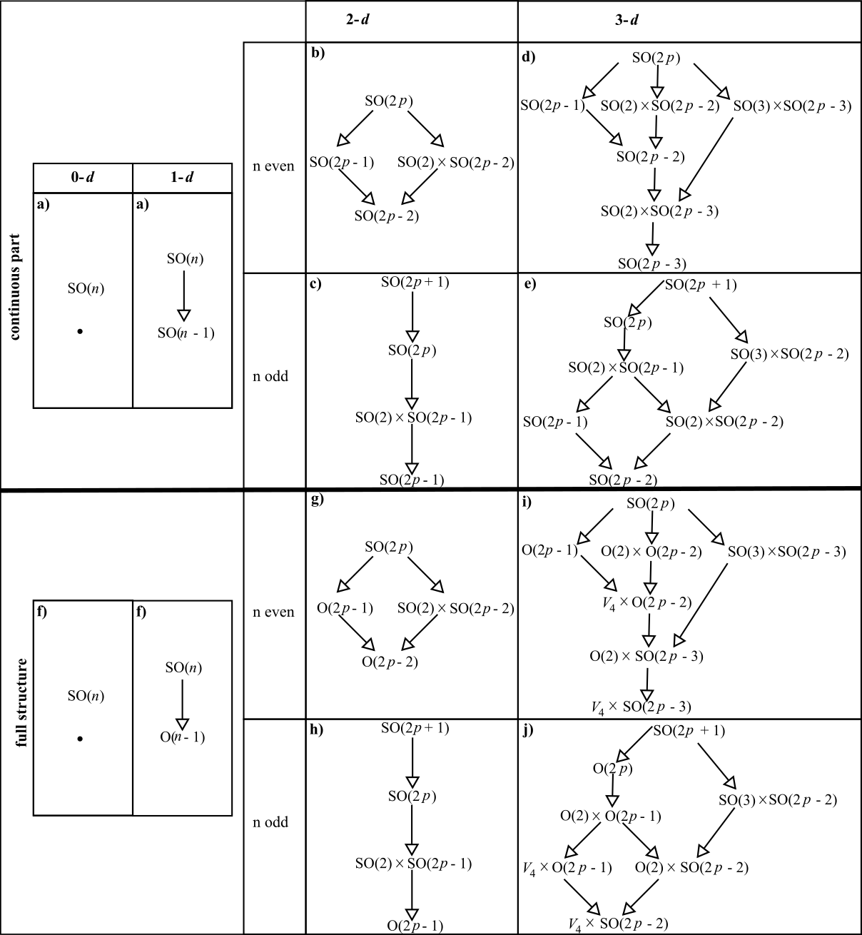
Figure 3: The general lattices.

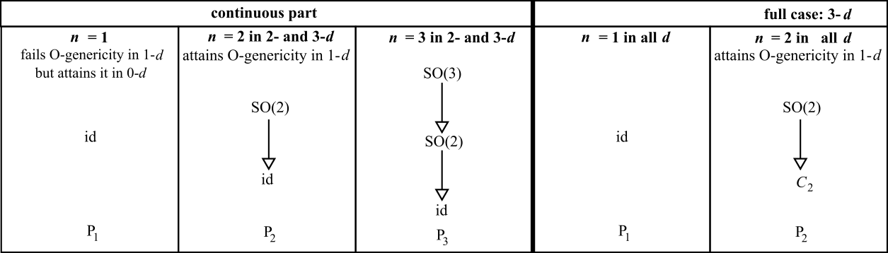
Figure 4: The exceptional cases’ $k$-chains $P_{k}$ of isotropy subgroups in 0-, 1- and 2-$d$

The even–odd distinction of these lattices in 2- and 3-$d$ follows from the number of Casimirs going up by one for every even $SO(n)$ but not at all for every odd $SO(n)$. Thus

$$SO(2\,p-1)\mbox{ }\leq\mbox{ }SO(2\,p)$$ (122)

leaves one Casimir unused, which can be used to generate an extra $SO(2)$, so

$$SO(2)\times SO(2\,p-1)\mbox{ }\leq\mbox{ }SO(2\,p)\mbox{ }.$$ (123)

On the other hand,

$$SO(2\,p-2)\mbox{ }\leq\mbox{ }SO(2\,p-1)$$ (124)

uses up all of the Casimirs, so an extra $SO(2)$ subgroup cannot be included.

We can place a sequence of qualitative criteria in terms of increasing complexity of the bounded lattice of isotropy subgroups as follows.

For arbitarary $d$, $N=2$’s isotropy subgroup lattice is only a point.

$N=3$’s isotropy subgroup lattice is the first with a distinct top and bottom but has no middle. In 1-$d$, this attains genericity.

$N=4$’s isotropy subgroup lattice is the first to have a middle but is still just a chain.

$N=5$’s isotropy subgroup lattice is the first with a nontrivial – rather than just chain – middle.

Proposition 3 Realizing the generic lattice of the continuous parts of the isotropy subgroups requires $N=4$ in 2-$d$ and $N=8$ in 3-$d$.

Proposition 4 i) For $d\neq 3$,

$$n=2\,d\mbox{ }\mbox{ ( i.e. \ $N=2\,d+1$ ) }$$ (125)

is an upper bound (‘B-genericity’, with ‘B’ standing for bounding) on O-genericity.

ii) For $d=3$, $n=7$ is required.

We need $d=0$, $n=0$, $d=1$, $n=2$ and $d=2$, $n=4$. The 3-$d$ case’s exceptionality is rooted in the

$$so(4)\mbox{ }=\mbox{ }so(3)\times so(3)$$ (126)

accidental relation.

9 Conclusion

We consider orbits and isotropy groups for $N$-body problems in 0, 1 and 2-$d$. This complements [41, 69]’s coverage of the 3-$d$ case, particularly in the light of [69, 71]’s detailed study of $N$’s interplay with $d$. For Mitchell and Littlejohn’s [41] notion that we term C-genericity – ‘C’ for ‘counting’ – 2, 3 and 4 Body Problems are minimal in dimensions 0, 1 and 2. For the Author’s notion of O-genericity (‘O’ for order-theoretic, referring to the bounded lattice of isotropy subgroups), 2, 3 and 5 Body problems are minimal in these dimensions. This 2 is an exception to the $N=2\,d+1$ rule, due to having only one object to order providing a more stringent bound. 3 is moreover also an exception by the Lie group accidental relation 126. We also tabulated the isotropy groups and orbit topologies and geometries for our small-$N$ Body Problems in dimensions 0, complementing [41] and making use of [69]’s observation that Stiefel and Grassmann spaces occur in bottom and top roles.

Applications include the following.

1) that some of the increase in complexity in passing from 3 to 4 and 5 body problems in 3-$d$ is already present in the more-well known setting of passing from intervals to triangles and then to quadrilaterals in 2-$d$.

2) That not (3, 6) but (4, 6) is a natural theoretical successor of (3, 5); however, we leave this, and other higher-$d$ $N$-Body Problems for subsequent occasions.

3) Such consideration isotropy groups and orbits is moreover a model for a larger case of interest, namely that of GR’s reduced configuration spaces.

We finally comment that, at the level of shapes, for 2-$d$ triangles the equal-eigenvalue case is regular to the non-equal eigenvalue case being irregular = tall-or-flat. Regular here means that the mass-weighted partial moments of inertia of the base and median are equal [49, 65]. Without mass weighting, these are in the proportion found in the equilateral triangle. The 2-$d$ quadrilaterals are moreover characterized by consideration of pairwise regularities in the subsystems formed by ignoring one of the three Jacobi separations that the quadrialteral’s frame supports [50, 63, 69].

Acknowledgments I thank Chris Isham and Don Page for concrete discussions about configuration space topology, geometry and background independence. I thank Don, Jeremy Butterfield, Malcolm MacCallum, Enrique Alvarez and Reza Tavakol for support with my career.

References

- [1]
- [2] G.W. Leibniz, The Metaphysical Foundations of Mathematics (University of Chicago Press, Chicago 1956) originally dating to 1715; The Leibnitz–Clark Correspondence, ed. H.G. Alexander (Manchester 1956), originally dating to 1715 and 1716.
- [3] E. Mach, Die Mechanik in ihrer Entwickelung, Historisch-kritisch dargestellt (Barth, Leipzig 1883). An English translation is The Science of Mechanics: A Critical and Historical Account of its Development Open Court, La Salle, Ill. 1960).
- [4] F.R. Moulton, “The Straight Line Solutions of Bodies", Ann. Math. 12 1 (1910).
- [5] J.L. Anderson, “Relativity Principles and the Role of Coordinates in Physics.", in Gravitation and Relativity ed. H-Y. Chiu and W.F. Hoffmann p. 175 (Benjamin, New York 1964).
- [6] P.A.M. Dirac, Lectures on Quantum Mechanics (Yeshiva University, New York 1964).
- [7] J.L. Anderson, Principles of Relativity Physics (Academic Press, New York 1967).
- [8] B.S. DeWitt, “Quantum Theory of Gravity. I. The Canonical Theory.", Phys. Rev. 160 1113 (1967).
- [9] J.A. Wheeler, in Battelle Rencontres: 1967 Lectures in Mathematics and Physics ed. C. DeWitt and J.A. Wheeler (Benjamin, New York 1968).
- [10] S. Smale “Topology and Mechanics. II. The Planar -Body Problem, Invent. Math. 11 45 (1970).
- [11] B.S. DeWitt, “Spacetime as a Sheaf of Geodesics in Superspace", in Relativity (Proceedings of the Relativity Conference in the Midwest, held at Cincinnati, Ohio June 2-6, 1969), ed. M. Carmeli, S.I. Fickler and L. Witten (Plenum, New York 1970).
- [12] A.E. Fischer, “The Theory of Superspace", in Relativity (Proceedings of the Relativity Conference in the Midwest, held at Cincinnati, Ohio June 2-6, 1969), ed. M. Carmeli, S.I. Fickler and L. Witten (Plenum, New York 1970).
- [13] R. McGehee, “Triple Collision in the Collinear Three-Body Problem", Invent. Math. 27 191 (1974).
- [14] J.N. Mather and R. McGehee, “Solutions of the Collinear Four Body Problem which Become Unbounded in Finite Time" in Dynamical Systems, Theory and Applications (Springer, Berlin 1975).
- [15] J. Palmore, “Measure of Degenerate Relative Equilibria, I. Annals of Math. 104 421 (1976).
- [16] J.B. Barbour and B. Bertotti, “Mach’s Principle and the Structure of Dynamical Theories", Proc. Roy. Soc. Lond. A382 295 (1982).
- [17] C. Nash and S. Sen, Topology and Geometry for Physicists (1983, Reprint by Dover, New York 2011).
- [18] M. Nakahara, Geometry, Topology and Physics (Institute of Physics Publishing, London 1990).
- [19] Z. Xia, The Existence of Noncollision Singularities in Newtonian Systems, Ann. Math. 135 411 (1992).
- [20] R. Moeckel, “Celestial Mechanics – Especially Central Configurations", http://www.math.umn.edu/ rmoeckel/notes/Notes.html (1994).
- [21] A. Albouy, Recherches sur le Probleme des N Corps (Habilitation, Bureau des Longitudes Paris 1995).
- [22] D.G. Kendall, “Shape Manifolds, Procrustean Metrics and Complex Projective Spaces", Bull. Lond. Math. Soc. 16 81 (1984).
- [23] D.G. Kendall, “A Survey of the Statistical Theory of Shape", Statistical Science 4 87 (1989).
- [24] C. Marchal, Celestial Mechanics (Elsevier, Tokyo 1990).
- [25] M. Henneaux and C. Teitelboim, Quantization of Gauge Systems (Princeton University Press, Princeton 1992).
- [26] K.V. Kuchař, “Time and Interpretations of Quantum Gravity", in Proceedings of the 4th Canadian Conference on General Relativity and Relativistic Astrophysics ed. G. Kunstatter, D. Vincent and J. Williams (World Scientific, Singapore, 1992), reprinted as Int. J. Mod. Phys. Proc. Suppl. D20 3 (2011).
- [27] C.J. Isham, “Canonical Quantum Gravity and the Problem of Time", in Integrable Systems, Quantum Groups and Quantum Field Theories ed. L.A. Ibort and M.A. Rodríguez (Kluwer, Dordrecht 1993), gr-qc/9210011.
- [28] D. Husemoller, Fibre Bundles (Springer, New York 1994).
- [29] R.G. Littlejohn and M. Reinsch, “Internal or Shape Coordinates in the -Body Problem", Phys. Rev. A52 2035 (1995).
- [30] V. Aquilanti, L. Bonnet and S. Cavalli, “Kinematic Rotations for Four-Centre Reactions: Mapping Tetra-Atomic Potential Energy Surfaces on the Kinetic Sphere", Mol. Phys. 89 1 (1996).
- [31] C.G.S. Small, The Statistical Theory of Shape (Springer, New York, 1996).
- [32] A.E. Fischer and V. Moncrief, “A Method of Reduction of Einstein’s Equations of Evolution and a Natural Symplectic Structure on the Space of Gravitational Degrees of Freedom", Gen. Rel. Grav. 28, 207 (1996).
- [33] R.G. Littlejohn and M. Reinsch, “Gauge Fields in the Separation of Rotations and Internal Motions in the -Body Problem", Rev. Mod. Phys. 69 213 (1997).
- [34] R.G. Littlejohn, K.A. Mitchell, M. Reinsch, V. Aquilanti and S. Cavalli, “Internal Spaces, Kinematic Rotations, and Body Frames for Four-Atom Systems", Phys. Rev. A 58 3718 (1998).
- [35] G. Sparr, “Euclidean and Affine Structure/Motion for Uncalibrated Cameras from Affine Shape and Subsidiary Information", in Proceedings of SMILE Workshop on Structure from Multiple Images, Freiburg (1998).
- [36] D.G. Kendall, D. Barden, T.K. Carne and H. Le, Shape and Shape Theory (Wiley, Chichester 1999).
- [37] G.E. Roberts, “A Continuum of Relative Equilibria in the Five-Body Problem", Phys. D127 141 (1999).
- [38] K.V. Mardia and P.E. Jupp, Directional Statistics (Wiley, Chichester 2000).
- [39] Y. Choquet-Bruhat and C. DeWitt-Morette, Analysis, Manifolds and Physics Vol. 2 (Elsevier, Amsterdam 2000).
- [40] P.M. Cohn, Classic Algebra (Wiley, Chichester 2000).
- [41] K.A Mitchell and R.G. Littlejohn, “Kinematic Orbits and the Structure of the Internal Space for Systems of Five or More Bodies", J. Phys. A: Math. Gen. 33 1395 (2000).
- [42] R. Montgomery, “Infinitely Many Syzygies", Arch. Rat. Mech. Anal. 164 311 (2002). “Fitting Hyperbolic Pants to a 3-Body Problem", Ergod. Th. Dynam. Sys. 25 921 (2005), math/0405014. “The Three-Body Problem and the Shape Sphere", Amer. Math. Monthly 122 299 (2015), arXiv:1402.0841.
- [43] K.V. Mardia and V. Patrangenaru, “Directions and Projective Shapes", Annals of Statistics 33 1666 (2005), math/0508280.
- [44] D. Giulini, “Some Remarks on the Notions of General Covariance and Background Independence", in An Assessment of Current Paradigms in the Physics of Fundamental Interactions ed. I.O. Stamatescu, Lect. Notes Phys. 721 105 (2007), arXiv:gr-qc/0603087.
- [45] D. Giulini, “The Superspace of Geometrodynamics", Gen. Rel. Grav. 41 785 (2009) 785, arXiv:0902.3923.
- [46] D. Groisser, and H.D. Tagare, “On the Topology and Geometry of Spaces of Affine Shapes", Journal of Mathematical Imaging and Vision 34 222 (2009).
- [47] E. Anderson, “The Problem of Time in Quantum Gravity", in Classical and Quantum Gravity: Theory, Analysis and Applications ed. V.R. Frignanni (Nova, New York 2012), arXiv:1009.2157.
- [48] T. Frankel, The Geometry of Physics: An Introduction (Cambridge University Press, Cambridge 2011).
- [49] E. Anderson, “The Problem of Time and Quantum Cosmology in the Relational Particle Mechanics Arena", arXiv:1111.1472.
- [50] E. Anderson, “Relational Quadrilateralland. I. The Classical Theory", Int. J. Mod. Phys. D23 1450014 (2014), arXiv:1202.4186.
- [51] A. Albouy and V. Kaloshin, “Finiteness of Central Configurations of Five Bodies in the Plane", Ann. Math. 176 535 (2012).
- [52] E. Anderson, “Problem of Time in Quantum Gravity", Annalen der Physik, 524 757 (2012), arXiv:1206.2403.
- [53] A. Bhattacharya and R. Bhattacharya, Nonparametric Statistics on Manifolds with Applications to Shape Spaces (Cambridge University Press, Cambridge 2012).
- [54] E. Anderson, “Background Independence", arXiv:1310.1524.
- [55] E. Anderson, “Beables/Observables in Classical and Quantum Gravity", SIGMA 10 092 (2014), arXiv:1312.6073.
- [56] E. Anderson, “Problem of Time and Background Independence: the Individual Facets", arXiv:1409.4117.
- [57] E. Anderson, “Spaces of Spaces", arXiv.1412.0239.
- [58] E. Anderson, “Six New Mechanics corresponding to further Shape Theories", Int. J. Mod. Phys. D 25 1650044 (2016), arXiv:1505.00488.
- [59] I.L. Dryden, K.V. Mardia, Statistical Shape Analysis, 2nd Edition (Wiley, Chichester 2016).
- [60] V. Patrangenaru and L. Ellingson, “Nonparametric Statistics on Manifolds and their Applications to Object Data Analysis" (Taylor and Francis, Boca Raton, Florida 2016).
- [61] F. Kelma, J.T. Kent and T. Hotz, “On the Topology of Projective Shape Spaces", arXiv:1602.04330.
- [62] E. Anderson, “A Local Resolution of the Problem of Time", arXiv:1809.01908; E. Anderson, The Problem of Time, Fundam.Theor.Phys. 190 (2017) pp.- ; alias The Problem of Time. Quantum Mechanics versus General Relativity, (Springer, New York 2017); its extensive Appendix Part “Mathematical Methods for Basic and Foundational Quantum Gravity", is freely accessible at https://link.springer.com/content/pdf/bbm3A978-3-319-58848-32F1.pdf .
- [63] E. Anderson, “The Smallest Shape Spaces. I. Shape Theory Posed, with Example of 3 Points on the Line", arXiv:1711.10054;
- [64] E. Anderson, “The Smallest Shape Spaces. II. 4 Points on a Line Suffices for a Complex Background-Independent Theory of Inhomogeneity", arXiv:1711.10073.
- [65] E. Anderson, “The Smallest Shape Spaces. III. Triangles in the Plane and in 3-", arXiv:1711.10115;
- [66] E. Anderson, “Alice in Triangleland: Lewis Carroll’s Pillow Problem and Variants Solved on Shape Space of Triangles", arXiv:1711.11492; “Two New Perspectives on Heron’s Formula", arXiv:1712.01441; “Maximal Angle Flow on the Shape Sphere of Triangles", arXiv:1712.07966. “Absolute versus Relational Debate: a Modern Global Version", arXiv:1805.09459; “Quadrilaterals in Shape Theory. II. Alternative Derivations of Shape Space: Successes and Limitations", cosubmitted to arXiv.
- [67] E. Anderson, “Specific PDEs for Preserved Quantities in Geometry. I. Similarities and Subgroups", arXiv:1809.02045.
- [68] E. Anderson, “Spaces of Observables from Solving PDEs. I. Translation-Invariant Theory.", arXiv:1809.07738;
- [69] E. Anderson “-Body Problem: Minimal for Qualitative Nontrivialities", arXiv:1807.08391.
- [70] E. Anderson, “Quadrilaterals in Shape Theory. II. Alternative Derivations of Shape Space: Successes and Limitations", co-submitted to arXiv.
- [71] E. Anderson “-Body Problem: Minimal for Qualitative Nontrivialities II: Varying Carrier Space and Group Quotiented Out", forthcoming October 2018.
- [72] E. Anderson, forthcoming.