Low-Energy Lepton-Proton Bremsstrahlung via Effective Field Theory

Abstract

We present a systematic calculation of the cross section for the lepton-proton bremsstrahlung process $l+p\to l^{\prime}+p+\gamma$ in chiral perturbation theory at next-to-leading order. This process corresponds to an undetected background signal for the proposed MUSE experiment at PSI. MUSE is designed to measure elastic scattering of low-energy electrons and muons off a proton target in order to extract a precise value of the proton’s r.m.s. radius. We show that the commonly used peaking approximation, which is used to evaluate the radiative tail for the elastic cross section, is not applicable for muon-proton scattering at the low-energy MUSE kinematics. Furthermore, we point out a certain pathology with the standard chiral power counting scheme associated with electron scattering, whereby the next-to-next-to-leading order contribution from the pion loop diagrams is kinematically enhanced and numerically of the same magnitude as the next-to-leading order corrections. We correct a misprint in a commonly cited review article.

I Introduction

Recent high precision experimental determinations of the proton’s r.m.s. radius have produced results which are not consistent with earlier results pohl10 ; Mohr2012 ; pohl13 . The proton radius puzzle refers to the contrasting results obtained between the proton’s electric charge radii extracted from the Lamb shift of muonic hydrogen atoms and those extracted from electron-proton scattering measurements, [see, e.g., Refs. Bernauer2010 ; Zhan2011 ; Mihovilovic2017 .] We note that a dispersion relation analysis of the proton form factor determined from electron-proton scattering data favors a charge radius Ulf1 ; Ulf2 consistent with that extracted from the experimental muonic hydrogen result. In order to resolve this issue, a number of newly commissioned experiments are underway, along with proposals of redoing the lepton-proton scattering measurements at low momentum transfers. The latter includes the MUon-proton Scattering Experiment (MUSE) gilman13 . The MUSE collaboration proposes to measure the elastic differential cross sections for $e^{\pm}p$ and $\mu^{\pm}p$ scattering at very low momentum transfers with an anticipated accuracy of a few tenths of a percent. This should allow for a very precise determination of the slope of the proton’s electric form factor $G^{p}_{E}$, and thereby, extract a value for the proton’s r.m.s. charge radius squared, $(r^{p}_{E})^{2}=\left.6\frac{\partial G^{p}_{E}(\tau^{2})}{\partial\tau^{2}}\right|_{\tau^{2}=0}$, where $\tau$ is the four-momentum transferred to the proton. The MUSE collaboration aims for an r.m.s. radius uncertainty of about 0.01 fm. However, in MUSE only the lepton scattering angle $\theta$ is detected. The final scattered lepton energy $E_{l}^{\prime}$ is not measured, nor are the bremsstrahlung photons. The bremsstrahlung photons constitute an integral part of the lepton-proton elastic scattering, and is one of the principal sources of uncertainties in the accurate measurement of the momentum transfers. In order to determine the proton charge radius, the data analysis necessarily needs to correct for this radiation process.

The lepton beam momenta considered by MUSE are of the order of the muon mass gilman13 ; LinLi . A particular concern is the standard radiative correction procedure, which makes use of the so-called peaking approximation, [see, e.g., Refs. maximon1969 ; maximon00 ; tsai1961 ; motsai1969 for reviews]. This approximation assumes that the bremsstrahlung photons are emitted either along the incident beam direction, or in the direction of the scattered final lepton momentum. The validity of this approximation normally relies on elastic scattering of highly relativistic particles, like electrons. This is, however, questionable when either the particle energy is comparable to its mass, e.g., in the case of low-energy muon scattering in MUSE, or for inelastic scatterings with large energy losses (30-40%) from the incident projectiles due to bremsstrahlung motsai1969 . The main purpose of this paper is to accurately assess the bremsstrahlung processes from electron and muon scattering off a proton at low energies in a model independent formalism. We show in a pedagogical manner the radical differences between the electron and muon angular bremsstrahlung spectra. We also correct a misprint in Eq. (B.5) of Ref. motsai1969 , which is important in the low-energy lepton scattering processes.

At low energies, which includes the kinematic region for MUSE, hadrons are the relevant degrees of freedom where the dynamics are governed by chiral symmetry requirements. Heavy Baryon Chiral Perturbation Theory ($\chi$PT) is a low-energy hadronic effective field theory (EFT), which incorporates the underlying symmetries and symmetry breaking patterns of QCD. In $\chi$PT the evaluation of observables follow well-defined chiral power counting rules, which determine the dominant leading order (LO) contributions, as well as the next-to-leading order (NLO) and higher order corrections to observables in a perturbative scheme. For example, in $\chi$PT the proton’s r.m.s. radius enters at next-to-next-to-leading order (NNLO) where pion loops at the proton-photon vertex enter into the calculation, see, e.g., Ref. bernard1995 . We note that $\chi$PT naturally includes the photon-hadron coupling in a gauge invariant way.

As mentioned, the goal of the present paper is to provide a pedagogical and model independent presentation of the bremsstrahlung process in a low-energy EFT framework. We will show how the lepton mass will crucially influence the photon’s angular distribution, and also discuss how the radiative tail cross section d$\sigma$/(d$p^{\prime}$d$\Omega^{\prime})$ depends on the outgoing lepton momentum $p^{\prime}$ and its mass $m_{l}$. We demonstrate that the so-called peaking approximation is not applicable for muon scattering at MUSE momenta. In fact, our results corroborate the analysis in Ref. ent01 , where it was shown that the peaking approximation, which is predominantly valid in the zero-mass limit or for very high-momentum transfers, becomes questionable at lower energies and could lead to significant errors in estimating the low-energy radiative cross sections. In this work we present a systematic evaluation the bremsstrahlung process using $\chi$PT up to and including NLO in chiral counting. Furthermore, we provide a rough estimate the NNLO contributions from the proton’s structure effects that arise from pion loop corrections to the LO proton-photon vertex. These NNLO pion loop contributions effectively introduce the proton’s r.m.s. radius, the first momentum dependent term in the charge form factor of the proton. As we shall discuss, contrary to the expectations based on standard chiral power counting for this process, the NNLO pion loop contributions appear to be kinematically enhanced by the small electron mass and roughly of the same order as the NLO contributions. This interesting observation, that emerges from our analysis in the case of the electron scattering, is not manifested in the case of the muon scattering due to the much larger muon mass.

The paper is organized as follows: In Sec. II we present a brief description of the lepton-proton bremsstrahlung process and the associated kinematics in the context of $\chi$PT, which, in principle, allows an order by order perturbative evaluation of the radiative and proton recoil correction contributions. In Sec. III we define the coordinate system and discuss the kinematics that are used in our evaluations of the analytic expressions for the differential cross sections. In Sec. IV, we present the results for our systematic evaluation up to and including NLO in chiral power counting. Sec. V contains a discussion of our numerical results. We furthermore include an estimate of the NNLO pion loop corrections, and present a comparison of these NNLO results with our full NLO evaluations. Finally, a short summary is presented before drawing some conclusions. For the sake of completeness we have added an appendix containing explicitly some of our elaborate expressions for the NLO amplitudes.

II Low-Energy Lepton-Proton Bremsstrahlung

In our evaluation the standard relativistic lepton-current BjDr is given by the expression

$$J^{\mu}_{l}(Q)=e\bar{u}_{l}(p^{\prime}_{l})\gamma^{\mu}u_{l}(p_{l})\,,$$ (1)

where $e=\sqrt{4\pi\alpha}$, and the four-momentum transferred to the proton is $Q=p_{l}-p^{\prime}_{l}$. The lepton mass is included in all our expressions, and we will show that the lepton mass plays a crucial role in determining the shape of the low-energy lepton-proton bremsstrahlung differential cross section. The hadronic current is derived from the $\chi$PT Lagrangian. In $\chi$PT it is assumed that the LO terms give the dominant contributions to the amplitude, while the higher chiral orders contribute smaller corrections to the LO amplitude. The effective $\chi$PT Lagrangian ${\mathcal{L}}_{\chi}$ is expanded in increasing chiral order as

$${\mathcal{L}}_{\chi}={\mathcal{L}}^{(0)}_{\pi N}+{\mathcal{L}}^{(1)}_{\pi N}+{\mathcal{L}}^{(2)}_{\pi N}+{\mathcal{L}}^{(0)}_{\pi\pi}+\cdots\;,$$ (2)

where the superscript in ${\mathcal{L}}^{(\nu)}$ denotes interaction terms of chiral order $\nu$. The proton mass $m_{p}$ is large, of the order of the chiral scale $\Lambda_{\chi}\sim 4\pi f_{\pi}\sim 1$ GeV, where $f_{\pi}=93$ MeV is the pion decay constant. An integral part of $\chi$PT is the expansion of the Lagrangian in powers of $m_{p}^{-1}$, where at LO, i.e., ${\cal L}^{(0)}_{\pi N}$, the proton is assumed static ($m_{p}\to\infty$). Note that in our evaluation the $m_{p}^{-1}$ corrections to the bremsstrahlung process have two different origin, namely, the kinematic phase-space corrections, as seen in Eqs. (10) and (11) below, and the dynamical $m_{p}^{-1}$ NLO corrections that arise from the photon-proton interaction in ${\cal L}_{\pi N}^{(1)}$, Eq.(2). In particular, it should be mentioned that in general the anomalous magnetic moments of the nucleons formally enter into the $\chi$PT calculations at NLO through ${\cal L}_{\pi N}^{(1)}$.

We first evaluate the LO contributions to the lepton-proton bremsstrahlung process shown in Fig. 1, using the explicit expression for the LO Lagrangian ${\mathcal{L}}^{(0)}_{\pi N}$ relevant for the processes under study, namely bernard1995 ; fettes00 ,

$$\mathcal{L}^{(0)}_{\pi N}=\bar{N}(iv\cdot D+g_{A}S\cdot u)N\,\,;\,\,u_{\mu} = iu^{\dagger}\nabla_{\mu}Uu^{\dagger}\,.$$ (3)

Here $N$ denotes the heavy nucleon spinor field and $g_{A}=1.26$ is the nucleon axial vector coupling constant, which does not contribute to our amplitude at LO and NLO. It is convenient to choose the proton four-velocity to be $v^{\mu}=(1,{\vec{0}})$ which determines the covariant proton spin operator to be $S^{\mu}=(0,\frac{1}{2}\vec{\sigma})$. The covariant derivative $D_{\mu}$ and $\nabla_{\mu}$ in Eq. (3) are defined as

$$D_{\mu} = \partial_{\mu}+\Gamma_{\mu}-iv^{(s)}_{\mu};$$

$$\Gamma_{\mu} = \frac{1}{2}[u^{\dagger}(\partial_{\mu}-ir_{\mu})u+u(\partial_{\mu}-il_{\mu})u^{\dagger}]\,,$$ (4)

$$\nabla_{\mu}U = \partial_{\mu}U-ir_{\mu}U+iUl_{\mu}\,.$$ (5)

The photon field ${\mathcal{A}}_{\mu}(x)$ is the only external source in this work, and the iso-scalar part of the photon field enters as $v^{(s)}_{\mu}(x)=-e\frac{I}{2}{\mathcal{A}}_{\mu}(x)$, where $I$ is the identity SU(2) matrix. The chiral connection $\Gamma_{\mu}$ and the chiral vielbein $u_{\mu}$ include the external iso-vector sources $r_{\mu}(x)$ and $l_{\mu}(x)$. In our work the left- and right- handed sources become $r_{\mu}(x)=l_{\mu}(x)=-e\frac{\tau_{3}}{2}{\mathcal{A}}_{\mu}(x)$. Generally, the $U$-field depends non-linearly on the pion field ${\bm{\pi}}$, and in the so-called “sigma”-gauge has the following form: $U(x)\equiv u^{2}(x)=\sqrt{1-{\bm{\pi}}^{2}/f_{\pi}^{2}}+i{\bm{\tau}}\cdot{\bm{\pi}}/f_{\pi}$. It may be noted that $U(x)=1$ at the LO where explicit pion fields are absent. The pion fields in $U(x)$ only enters the calculation to generate the NNLO pion loop contributions, see later. We adopt the Coulomb gauge, i.e., $\epsilon\cdot v=0$, where $\epsilon^{\mu}$ is the outgoing photon polarization four-vector. This implies that in $\chi$PT the bremsstrahlung photon from the proton, diagrams (C) and (D) in Fig. 1, do not contribute to the bremsstrahlung process at LO.

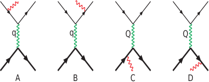
Figure 1: Feynman diagrams contributing to lepton-proton bremsstrahlung process. In the Coulomb gauge the proton radiation diagrams (C) and (D) do not contribute at the leading order in $\chi$PT.

The first non-trivial contribution of photon radiation from proton [Feynman diagrams (G) and (H) in Fig. 2] arises from the NLO interactions specified by ${\cal L}^{(1)}_{\pi N}$ in Eq.(2). Like diagrams (C) and (D) in Fig. 1, diagrams (I) and (J) in Fig. 2 do not contribute in the Coulomb gauge. For completeness, we also specify the NLO Lagrangian bernard1995 ; fettes00 , where, however, only the terms directly relevant to our analysis are retained.

$${\cal L}^{(1)}_{\pi N} = \bar{N}\frac{1}{2m_{p}}\biggl{\{}(v\cdot D)^{2}-D\cdot D-\frac{i}{2}\left[S^{\mu},S^{\nu}\right]$$ (6)

$$\times\biggl{[}(1+\kappa_{v})f^{+}_{\mu\nu}+2(1+\kappa_{s})v^{(s)}_{\mu\nu}\biggr{]}+\cdots\biggr{\}}N\,.$$

Here

$$f^{+}_{\mu\nu} = u^{\dagger}F^{R}_{\mu\nu}u+uF^{L}_{\mu\nu}u^{\dagger}$$ (7)

$$= -e\left(\partial_{\mu}{\mathcal{A}}_{\nu}-\partial_{\nu}{\mathcal{A}}_{\mu}\right)(u^{\dagger}{\mathcal{Q}}u+u{\mathcal{Q}}u^{\dagger}),$$

where ${\mathcal{Q}}={\rm diag}(1,0)$ is the nucleon charge matrix, and

$$F^{L}_{\mu\nu} = F^{R}_{\mu\nu}=\partial_{\mu}l_{\nu}-\partial_{\nu}l_{\mu}-i\left[l_{\mu},l_{\nu}\right]$$

$$= -e\frac{\tau_{3}}{2}\left(\partial_{\mu}{\mathcal{A}}_{\nu}-\partial_{\nu}{\mathcal{A}}_{\mu}\right),$$

$$v^{(s)}_{\mu\nu} = \partial_{\mu}v^{(s)}_{\nu}-\partial_{\nu}v^{(s)}_{\mu}=-e\frac{I}{2}\left(\partial_{\mu}{\mathcal{A}}_{\nu}-\partial_{\nu}{\mathcal{A}}_{\mu}\right)\,.$$ (8)

Since the bremsstrahlung cross section is proportional to $\alpha/m^{2}$ for a radiating particle of mass $m$, we expect the NLO contributions to be small compared to the LO due to the large proton mass.

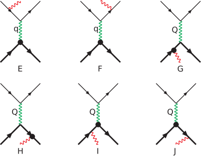
Figure 2: Feynman diagrams contributing to the lepton-proton bremsstrahlung process at NLO. The filled blobs represents insertion of proton-photon interaction terms from ${\cal L}_{\pi N}^{(1)}$. In the Coulomb gauge the proton radiation diagrams (I) and (J) do not contribute.

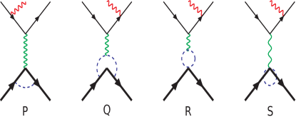
Figure 3: A subset of all NNLO Feynman diagrams of the lepton-proton bremsstrahlung process, where the pion loops, shown by the dashed (blue) propagator lines, contribute to the proton form factors. The vertices in the NNLO pion loop diagrams are all generated by ${\cal L}_{\pi N}^{(0)}$.

In $\chi$PT we naively expect that the NNLO corrections are of order $(\mathscr{P}/\Lambda_{\chi})^{3}\ll 1$, where $\mathscr{P}$ denotes the four-momentum of the process of the order of the pion mass, $m_{\pi}$. However, it turns out that the pion loop contributions are as important as the lower chiral order nucleon pole graph contributions. We will investigate the question regarding the magnitudes of the NNLO pion loop contributions in our process, i.e., we examine how well the usual chiral counting works for the lepton-proton bremsstrahlung process in Sec. V. At NNLO the Lagrangian ${\cal L}_{\pi N}^{(2)}$, can be written as ${\cal L}_{\pi N}^{(2)}={\mathscr{L}}^{(2),{\rm fixed}}_{\pi N}+{\mathscr{L}}^{(2)}_{\pi N}$, where ${\mathscr{L}}^{(2),{\rm fixed}}_{\pi N}$ contains $m_{p}^{-2}$ recoil terms with known coefficients, while ${\mathscr{L}}^{(2)}_{\pi N}$ contains low-energy constants (LECs). The LECs regularize the ultra-violet (UV) contributions from the pion loop diagrams, which enter at NNLO order. The pion loops associated with the photon-proton vertex in diagrams (A) and (B) of Fig. 1 are illustrated in Fig. 3. They contribute to the first momentum dependence of the proton form factors in $\chi$PT. In this work we will effectively make use of the NNLO proton electric form factor which along with the magnetic form factor was formally derived in Refs. fettes00 ; Bernard1998 ; hemmert1998 ; Ecker1994 using $\chi$PT. The explicit ${\cal L}_{\pi N}^{(2)}$ expression can also be found in those references. At this chiral order the measured r.m.s. charge and magnetic radii determine LECs in ${\cal L}_{\pi N}^{(2)}$ Bernard1998 . In essence, a measure of the NNLO contributions to our cross section is the following electric Sachs form factor $G^{p}_{E}$, expressed in terms of the corresponding iso-vector $G^{v}_{E}$ and iso-scalar $G^{s}_{E}$ form factors, namely

$$G^{p}_{E}(q^{2})=\frac{1}{2}\left[G^{v}_{E}(q^{2})+G^{s}_{E}(q^{2})\right]\approx 1+\frac{q^{2}}{6}(r^{p}_{E})^{2}+{\mathcal{O}}(q^{4}),$$

(9)

where $r^{p}_{E}$ is the electric radius of the proton. In Sec. V, our rough estimate of the NNLO contribution is obtained by folding the LO differential cross section results with $G^{p}_{E}$ which include the “measured” r.m.s. radius as the phenomenological input. These should effectively simulate the NNLO $\chi$PT pion loop contributions.

III The LO and NLO cross sections

At LO only the Feynman diagrams (A) and (B) in Fig. 1, contribute. We denote the incident and scattered lepton four-momenta as $p_{l}=(E_{l},\vec{p})$ and $p^{\prime}_{l}=(E^{\prime}_{l},\vec{p}^{\,\prime})$, respectively, where, e.g., $E_{l}=\sqrt{m_{l}^{2}+\vec{p}^{\,2}}$. The corresponding proton four-momenta are $P_{p}=(E_{p},\vec{P}_{p})$ and $P^{\prime}_{p}=(E^{\prime}_{p},\vec{P}^{\,\prime}_{p})$, and the outgoing photon has the four-momentum $k=(E_{\gamma},\vec{k})$. Furthermore, $\theta$ is the lepton scattering angle such that $\vec{p}\cdot\vec{p}^{\,\prime}=|\vec{p}\,||\vec{p}^{\,\prime}|{\rm cos}\theta$, and $q=(Q-k)$ is the four-momentum transferred to the proton when the lepton is radiating.

In $\chi$PT the non-relativistic heavy proton four-momentum satisfies re-parametrization invariance Bernard1992 ; Manohar , and takes the form $P^{\mu}_{p}=m_{p}v^{\mu}+p_{p}^{\mu}$, where $m_{p}$ is the proton mass, such that the square of its off-shell residual part is $p_{p}^{2}\ll m_{p}^{2}$. This means that the incident proton kinetic energy to lowest order in $m_{p}^{-1}$ becomes $v\cdot p_{p}=\frac{\vec{p}_{p}^{\,2}}{2m_{p}}+\cdots$, and similarly for the final recoiling proton. The bremsstrahlung differential cross section is given in the laboratory frame by the general expression

$${\rm d}\sigma = \int\frac{{\rm d}^{3}\vec{p}^{\,\prime}\;{\rm d}^{3}\vec{k}}{(2\pi)^{5}8E_{l}^{\prime}E_{\gamma}}\frac{\delta\left(E_{l}-E_{l}^{\prime}-E_{\gamma}-\frac{(\vec{p}-\vec{p}^{\,\prime}-\vec{k})^{2}}{2m_{p}}+\cdots\right)}{4m_{p}E_{l}\left(m_{p}+\frac{(\vec{p}-\vec{p}^{\,\prime}-\vec{k})^{2}}{2m_{p}}+\cdots\right)}\,$$ (10)

$$\quad\times\,\,\frac{1}{4}\sum_{\rm spins}|{\mathcal{M}}_{br}|^{2}\,,$$

where in the phase-space expression (including the $\delta$-function) we expand the recoil proton energy as

$$E^{\prime}_{p} = \sqrt{m^{2}_{p}+(\vec{p}^{\,\prime}_{p})^{2}}$$ (11)

$$= m_{p}+\frac{(\vec{p}-\vec{p}^{\,\prime}-\vec{k})^{2}}{2m_{p}}+{\mathcal{O}}\left(m^{-3}_{p}\right)\,.$$

A straightforward evaluation of the two Feynman diagrams (A) and (B), shown in Fig. 1 leads to the following LO expression for the bremsstrahlung amplitude squared:

$$\frac{1}{4}\sum_{\rm spins}\!\!|{\mathcal{M}}^{\rm(LO)}_{br}|^{2} = \frac{1}{4}\sum|{\mathcal{M}}_{A}+{\mathcal{M}}_{B}|^{2}=\left(\frac{512\pi^{3}\alpha^{3}}{q^{4}}\right)(m_{p}+E_{p})(m_{p}+E_{p}^{\prime})$$ (12)

$$\times\,\Biggl{\{}-\,\,\frac{1}{[(p^{\prime}+k)^{2}-m_{l}^{2}]^{2}}\left[m_{l}^{4}+m_{l}^{2}E_{l}^{\prime}E_{l}+m_{l}^{2}E_{l}E_{\gamma}+m_{l}^{2}E_{l}^{\prime}E_{\gamma}-E_{l}E_{l}^{\prime}E_{\gamma}^{2}+m_{l}^{2}(\vec{k}\cdot\vec{p})-m_{l}^{2}(\vec{k}\cdot\vec{p}^{\,\prime})\right.$$

$$\left.\hskip 125.75018pt+\,\,m_{l}^{2}(\vec{p}\cdot\vec{p}^{\,\prime})+E_{l}E_{\gamma}(\vec{k}\cdot\vec{p}^{\,\prime})-E_{l}^{\prime}E_{\gamma}(\vec{k}\cdot\vec{p})+(\vec{k}\cdot\vec{p}^{\,\prime})(\vec{k}\cdot\vec{p})\right]$$

$$\hskip 15.6491pt-\,\,\frac{1}{[(p-k)^{2}-m_{l}^{2}]^{2}}\left[m_{l}^{4}-E_{\gamma}^{2}E_{l}E_{l}^{\prime}+m_{l}^{2}E_{l}E_{l}^{\prime}-m_{l}^{2}E_{l}E_{\gamma}-m_{l}^{2}E_{l}^{\prime}E_{\gamma}+m_{l}^{2}(\vec{p}\cdot\vec{k})+m_{l}^{2}(\vec{p}\cdot\vec{p}^{\,\prime})\right.$$

$$\left.\hskip 125.75018pt-\,\,m_{l}^{2}(\vec{k}\cdot\vec{p}^{\,\prime})-E_{l}E_{\gamma}(\vec{k}\cdot\vec{p}^{\,\prime})+E_{l}^{\prime}E_{\gamma}(\vec{k}\cdot\vec{p})+(\vec{k}\cdot\vec{p}^{\,\prime})(\vec{k}\cdot\vec{p})\right]$$

$$\hskip 15.6491pt-\,\,\frac{2}{[(p^{\prime}+k)^{2}-m_{l}^{2}]\,[(p-k)^{2}-m_{l}^{2}]}\left[m_{l}^{2}E_{l}^{\prime}E_{l}-m_{l}^{2}E_{\gamma}^{2}+E_{l}^{2}E_{l}^{\prime 2}-m_{l}^{2}(\vec{p}\cdot\vec{p}^{\,\prime})+E_{l}^{2}(\vec{k}\cdot\vec{p}^{\,\prime})\right.$$

$$\left.\hskip 125.75018pt-\,\,E_{l}^{\prime\,2}(\vec{k}\cdot\vec{p})-(\vec{p}\cdot\vec{p}^{\,\prime})^{2}+(\vec{p}\cdot\vec{p}^{\,\prime})(\vec{k}\cdot\vec{p}^{\,\prime})-(\vec{p}\cdot\vec{p}^{\,\prime})(\vec{k}\cdot\vec{p}\,)\right]\,\,\Biggr{\}}\,.$$

To evaluate the cross section, it is convenient to define our reference frame such that the momentum transfer, $\vec{Q}=\vec{p}-\vec{p}^{\,\prime}$ is directed along the $z$-axis motsai1969 , while the lepton momenta, $\vec{p}$ and $\vec{p}^{\,\prime}$, lie in $xz$-plane as shown in Fig. 4. The pertinent angles are defined as follows:

$$\vec{k}\cdot\vec{p}^{\,\prime} = E_{\gamma}|\vec{p}^{\,\prime}|(\cos\gamma\,\cos\alpha+\sin\alpha\,\sin\gamma\,\cos\phi_{\gamma}),$$

$$\vec{k}\cdot\vec{p} = E_{\gamma}|\vec{p}\,|(\cos\zeta\,\cos\alpha+\sin\alpha\,\sin\zeta\,\cos\phi_{\gamma})\,.$$ (13)

The lepton scattering angle in our coordinate system is given as $\theta=\gamma-\zeta$. When the lepton radiates a photon the squared four-momentum transferred to the proton is

$$q^{2} = (Q-k)^{2}$$ (14)

$$= 2\biggl{[}m^{2}_{l}-E_{l}E_{l}^{\prime}+|\vec{p}\,||\vec{p}^{\,\prime}|\cos\theta-E_{\gamma}(E_{l}-E_{l}^{\prime})$$

$$+\,E_{\gamma}\cos\alpha\sqrt{|\vec{p}\,|^{2}+|\vec{p}^{\,\prime}|^{2}-2|\vec{p}\,||\vec{p}^{\,\prime}|\cos\theta}\biggr{]}\,,$$

which is independent of $\phi_{\gamma}$ in our reference frame as suggested in Ref. motsai1969 . This choice of reference frame readily allows the analytical $\phi_{\gamma}$ integration.

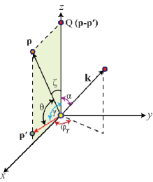
Figure 4: Reference coordinate system used in the evaluation of the differential cross section, such that $\vec{Q}=\vec{p}-\vec{p}^{\,\prime}$ is taken along the $z$-axis, while $\vec{p}$ and $\vec{p}^{\,\prime}$ lie in $xz$-plane. The different angles and three-momentum symbols are defined in the text.

To evaluate our LO expression for the differential cross section, ${\rm d}^{3}\sigma^{\rm(LO)}/({\rm d}|\vec{p}^{\,\prime}|\,{\rm d}\Omega^{\prime}_{l}\,{\rm d}{\rm cos}\alpha)$ [see Eq. (LABEL:eq:sigma5)], it is convenient to define two angle dependent parameters,

$$a=\frac{1-\beta^{\prime}\cos\alpha\,\cos\gamma}{\beta^{\prime}\sin\alpha\,\sin\gamma}\quad{\rm and}\quad b=\frac{1-\beta\cos\alpha\,\cos\zeta}{\beta\sin\alpha\,\sin\zeta}\,.$$

Here $\beta=\frac{|\vec{p}\,|}{E_{l}}$ and $\beta^{\prime}=\frac{|\vec{p}^{\,\prime}|}{E_{l}^{\prime}}$ are the incoming and outgoing lepton velocities, respectively. In this equation, we also define the magnitudes of the incoming and outgoing lepton three-momenta as $p=|\vec{p}|$ and $p^{\prime}=|\vec{p}^{\,\prime}|$, respectively. To obtain our final expression, we integrate the cross section in Eq. (10) over the photon energies $E_{\gamma}$, which means that the infrared singularity will appear when the momentum $p^{\prime}$ is close to it’s maximal allowed value. To account for the proton recoil corrections in the kinematics we include the $m_{p}^{-1}$ terms in the photon energy $E_{\gamma}$ given by the delta-function in Eq. (10). We define $E_{\gamma}^{0}=E_{l}-E_{l}^{\prime}$, which gives the following expression for $E_{\gamma}$,

$$E_{\gamma}=E_{\gamma}^{0}-\frac{K}{m_{p}}+{\mathcal{O}}\left(m^{-3}_{p}\right)\,,$$ (15)

where

$$K = \frac{1}{2}\biggl{[}|\vec{p}|^{2}+|\vec{p}^{\,\prime}|^{2}-2|\vec{p}||\vec{p}^{\,\prime}|\cos\theta+(E_{\gamma}^{0})^{2}$$ (16)

$$-\,2E_{\gamma}^{0}\cos\alpha\sqrt{|\vec{p}|^{2}+|\vec{p}^{\,\prime}|^{2}-2|\vec{p}||\vec{p}^{\,\prime}|\cos\theta}\biggr{]}\,.$$

When integrating over $E_{\gamma}$, the expression in the delta-function also introduces a factor $\left(1-\frac{Z}{m_{p}}\right)$ in the phase-space to lowest order in $m_{p}^{-1}$ needed in our analysis, where

$$Z=E_{\gamma}^{0}-\cos\alpha\,\sqrt{|\vec{p}|^{2}+|\vec{p}^{\,\prime}|^{2}-2|\vec{p}||\vec{p}^{\,\prime}|\cos\theta}.$$ (17)

Furthermore, the $m_{p}^{-1}$ correction in the photon energy affects the expression for the four-momentum transfer $q^{2}$, which can be written as

$$q^{2}=(q^{0})^{2}+\frac{\kappa}{m_{p}}+{\mathcal{O}}\left(m^{-3}_{p}\right)\,,$$ (18)

where

$$(q^{0})^{2} = 2\biggl{[}m^{2}_{l}-E_{l}E_{l}^{\prime}+|\vec{p}\,||\vec{p}^{\,\prime}|\cos\theta-E_{\gamma}^{0}(E_{l}-E_{l}^{\prime})$$ (19)

$$+\,E_{\gamma}^{0}\cos\alpha\sqrt{|\vec{p}\,|^{2}+|\vec{p}^{\,\prime}|^{2}-2|\vec{p}\,||\vec{p}^{\,\prime}|\cos\theta}\biggr{]},$$

and

$$\kappa=2K\Big{[}E_{l}-E_{l}^{\prime}-\cos\alpha\sqrt{|\vec{p}\,|^{2}+|\vec{p}^{\,\prime}|^{2}-2|\vec{p}\,||\vec{p}^{\,\prime}|\cos\theta}\Big{]}\,.$$

In the process of evaluation of the cross section up to NNLO, we will only need the $m_{p}^{-1}$ kinematic terms, i.e., we include the $m_{p}^{-1}$ corrections for $E_{\gamma}$, $q^{2}$, as well as in the above given phase-space factor.

As a pedagogical survey of the bremsstrahlung process at energies not much larger than the muon mass, we initially consider the most simplest and rather qualitative case of the static proton limit ($m_{p}\to\infty$). We shall then compare these qualitative results with the improved ones obtained by, first, including the kinematical $m_{p}^{-1}$ recoil corrections in the phase space factor and the delta-function expression in Eq. (10), and second, by including the dynamical $m_{p}^{-1}$ recoil corrections in the matrix element at NLO.

As a first step, we evaluate the LO cross section in the static proton limit ($m_{p}\to\infty$), which is expressed as

$${\rm d}\sigma^{\rm(LO)}_{{\rm static}} = \int\frac{{\rm d}^{3}\vec{p}^{\,\prime}\,{\rm d}^{3}\vec{k}}{(2\pi)^{5}32E_{l}^{\prime}E_{\gamma}m_{p}^{2}E_{l}}\delta\left(E_{l}-E_{l}^{\prime}-E_{\gamma}\right)$$ (21)

$$\quad\times\,\,\frac{1}{4}\sum_{spin}|{\mathcal{M}}_{br}^{\rm static}|^{2}\,.$$

When we evaluate ${\mathcal{M}}_{br}^{\rm static}$ in Eq. (21) in the static proton limit ($m_{p}\to\infty$), we set $K$, $\kappa$ and $Z$ all equal zero in Eq. (LABEL:eq:sigma5). This equation incorporates the $m_{p}^{-1}$ recoil effects only from the phase space [including the energy-delta function in Eq. (10)] but the matrix element is derived from the leading chiral order Lagrangian ${\mathcal{L}}^{(0)}_{\pi N}$:

$$\frac{{\rm d}^{3}\sigma^{\rm(LO)}}{{\rm d}p^{\prime}\,{\rm d}\Omega^{\prime}_{l}\,{\rm d}\cos\alpha} = \left(\frac{\alpha^{3}\beta^{\prime\,2}}{2\pi^{2}q^{4}}\right)\left(1-\frac{Z}{m_{p}}\right)E_{\gamma}$$

$$\left\{-\int_{0}^{2\pi}{\rm d}\phi_{\gamma}\frac{1}{(a-\cos\phi_{\gamma})^{2}}\left(\frac{1}{E_{l}E^{\prime}_{l}E_{\gamma}^{2}(\beta^{\prime}\,{\sin}\alpha\,{\sin}\gamma)^{2}}\right)\right.$$

$$\left.\hskip 22.76228pt\times\,\Big{[}m_{l}^{4}-E_{l}E_{l}^{\prime}E_{\gamma}^{2}+m_{l}^{2}E_{l}^{\prime}E_{\gamma}+m_{l}^{2}E_{l}E_{l}^{\prime}+m_{l}^{2}E_{l}E_{\gamma}+m_{l}^{2}pp^{\prime}\cos\theta\right.$$

$$\left.\hskip 36.98866pt-\,m_{l}^{2}p^{\prime}E_{\gamma}\,\Big{(}{\cos}\alpha\,{\cos}\gamma+\,{\sin}\alpha\,{\sin}\gamma\,{\cos}\phi_{\gamma}\Big{)}+\,p^{\prime}E_{l}E_{\gamma}^{2}\,\Big{(}{\cos}\alpha\,{\cos}\gamma+\,{\sin}\alpha\,{\sin}\gamma\,{\cos}\phi_{\gamma}\Big{)}\right.$$

$$\left.\hskip 36.98866pt+\,m_{l}^{2}pE_{\gamma}\,\Big{(}{\cos}\alpha\,{\cos}\zeta+\,{\sin}\alpha\,{\sin}\zeta\,{\cos}\phi_{\gamma}\Big{)}-\,pE_{l}^{\prime}E_{\gamma}^{2}\,\Big{(}{\cos}\alpha\,{\cos}\zeta+\,{\sin}\alpha\,{\sin}\zeta\,{\cos}\phi_{\gamma}\Big{)}\right.$$

$$\left.\hskip 36.98866pt+\,pp^{\prime}E_{\gamma}^{2}\,\Big{(}{\cos}^{2}\alpha\,{\cos}\gamma\,{\cos}\zeta+\,{\cos}\alpha\,{\cos}\gamma\,{\sin}\alpha\,{\sin}\zeta\,{\cos}\phi_{\gamma}+\,{\sin}\alpha\,{\sin}\gamma\,{\cos}\alpha\,{\cos}\zeta\,{\cos}\phi_{\gamma}\right.$$

$$\left.\hskip 36.98866pt+\,{\sin}^{2}\alpha\,{\sin}\gamma\,{\sin}\zeta\,{\cos}^{2}\phi_{\gamma}\Big{)}\Big{]}_{{\rm dir}(\gamma)}\right.$$

$$\left.-\,\int_{0}^{2\pi}{\rm d}\phi_{\gamma}\frac{1}{(b-\cos\phi_{\gamma})^{2}}\left(\frac{E_{l}^{\prime}}{E_{l}^{3}E_{\gamma}^{2}(\beta\,{\sin}\alpha\,{\sin}\zeta)^{2}}\right)\right.$$

$$\left.\hskip 22.76228pt\times\,\Big{[}m_{l}^{4}-E_{l}E_{l}^{\prime}E_{\gamma}^{2}-m_{l}^{2}E_{l}^{\prime}E_{\gamma}+m_{l}^{2}E_{l}E_{l}^{\prime}-m_{l}^{2}E_{l}E_{\gamma}+m_{l}^{2}pp^{\prime}\cos\theta\right.$$

$$\left.\hskip 36.98866pt-\,m_{l}^{2}p^{\prime}E_{\gamma}\,\Big{(}{\cos}\alpha\,{\cos}\gamma+\,{\sin}\alpha\,{\sin}\gamma\,{\cos}\phi_{\gamma}\Big{)}-\,p^{\prime}E_{l}E_{\gamma}^{2}\,\Big{(}{\cos}\alpha\,{\cos}\gamma+\,{\sin}\alpha\,{\sin}\gamma\,{\cos}\phi_{\gamma}\Big{)}\right.$$

$$\left.\hskip 36.98866pt+\,m_{l}^{2}pE_{\gamma}\,\Big{(}{\cos}\alpha\,{\cos}\zeta+\,{\sin}\alpha\,{\sin}\zeta\,{\cos}\phi_{\gamma}\Big{)}+\,pE_{l}^{\prime}E_{\gamma}^{2}\,\Big{(}{\cos}\alpha\,{\cos}\zeta+\,{\sin}\alpha\,{\sin}\zeta\,{\cos}\phi_{\gamma}\Big{)}\right.$$

$$\left.\hskip 36.98866pt+\,pp^{\prime}E_{\gamma}^{2}\,\Big{(}{\cos}^{2}\alpha\,{\cos}\gamma\,{\cos}\zeta+\,{\cos}\alpha\,{\cos}\gamma\,{\sin}\alpha\,{\sin}\zeta\,{\cos}\phi_{\gamma}+\,{\sin}\alpha\,{\sin}\gamma\,{\cos}\alpha\,{\cos}\zeta\,{\cos}\phi_{\gamma}\right.$$

$$\left.\hskip 36.98866pt+\,{\sin}^{2}\alpha\,{\sin}\gamma\,{\sin}\zeta\,{\cos}^{2}\phi_{\gamma}\Big{)}\Big{]}_{{\rm dir}(\zeta)}\right.$$

$$\left.+\,\int_{0}^{2\pi}{\rm d}\phi_{\gamma}\frac{1}{(a-\cos\phi_{\gamma})(b-\cos\phi_{\gamma})}\left(\frac{2}{E_{l}^{2}E_{\gamma}^{2}(\beta\beta^{\prime}\,{\sin}^{2}\alpha\,{\sin}\gamma\,{\sin}\zeta)}\right)\right.$$

$$\left.\hskip 22.76228pt\times\,\Big{[}m_{l}^{2}E_{l}E_{l}^{\prime}+E_{l}^{2}E_{l}^{\prime 2}-m_{l}^{2}E_{\gamma}^{2}-\,m_{l}^{2}pp^{\prime}\cos\theta-p^{2}p^{\prime 2}\,{\cos}^{2}\theta\right.$$

$$\left.\hskip 36.98866pt+\,p^{\prime}E_{l}^{2}E_{\gamma}\,\Big{(}{\cos}\alpha\,{\cos}\gamma+\,{\sin}\alpha\,{\sin}\gamma\,{\cos}\phi_{\gamma}\Big{)}+\,pp^{\prime 2}E_{\gamma}\cos\theta\,\Big{(}{\cos}\alpha\,{\cos}\gamma+\,{\sin}\alpha\,{\sin}\gamma\,{\cos}\phi_{\gamma}\Big{)}\right.$$

$$\left.\hskip 36.98866pt-\,pE_{l}^{\prime 2}E_{\gamma}\,\Big{(}{\cos}\alpha\,{\cos}\zeta+\,{\sin}\alpha\,{\sin}\zeta\,{\cos}\phi_{\gamma}\Big{)}-\,p^{2}p^{\prime}E_{\gamma}\cos\theta\,\Big{(}{\cos}\alpha\,{\cos}\zeta+\,{\sin}\alpha\,{\sin}\zeta\,{\cos}\phi_{\gamma}\Big{)}\Big{]}_{\rm int}{\color[rgb]{1,1,1}\int_{0}^{2\pi}}\right\}\,.$$

The terms within the first and second square brackets, i.e., $[\cdots]_{{\rm dir}(\gamma)}$ and $[\cdots]_{{\rm dir}(\zeta)}$, represent the contributions from the “direct” terms (matrix element squared of diagram (B) and (A), respectively) of real photon emissions from the outgoing and incoming leptons, respectively. The third square bracket $[\cdots]_{\rm int}$, represents the “interference” contribution of diagrams (A) and (B).

Next including the ${\mathcal{O}}(m^{-1}_{p})$ dynamical corrections in the matrix elements due to the interactions in ${\cal L}^{(1)}_{\pi N}$, i.e., with

$$\left|\mathcal{M}_{br}\right|^{2} \to 2{\rm Re}\sum_{\rm spins}\left({\mathcal{M}}_{\rm A}+{\mathcal{M}}_{\rm B}\right)^{*}$$ (23)

$$\qquad\times\,\left({\mathcal{M}}_{\rm E}+{\mathcal{M}}_{\rm F}+{\mathcal{M}}_{\rm G}+{\mathcal{M}}_{\rm H}\right)\,,$$

yields the complete NLO expression to the bremsstrahlung differential cross section which is expressed as

$$\frac{{\rm d}^{3}\sigma}{{\rm d}p^{\,\prime}\,{\rm d}\Omega^{\prime}_{l}\,{\rm d}\cos\alpha} = \frac{{\rm d}^{3}\sigma^{\rm(LO)}}{{\rm d}p^{\,\prime}\,{\rm d}\Omega^{\prime}_{l}\,{\rm d}\cos\alpha}+\Delta\left[\frac{\rm d^{3}\sigma}{{\rm d}p^{\prime}\,{\rm d}\Omega_{l}^{\prime}\,{\rm d}\cos\alpha}\right]_{\rm NLO},$$

where the $\mathcal{O}(m^{-1}_{p})$ NLO correction term above is

$$\Delta\left[\frac{\rm d^{3}\sigma}{{\rm d}p^{\prime}\,{\rm d}\Omega_{l}^{\prime}\,{\rm d}\cos\alpha}\right]_{\rm NLO}\!\!\! = \left(\frac{\alpha^{3}\beta^{\prime 2}}{2\pi^{2}(q^{0})^{4}}\right)\frac{1}{m_{p}}2E^{0}_{\gamma}$$

$$\times\,\int^{2\pi}_{0}{\rm d}\phi_{\gamma}\Bigg{[}-\frac{1}{(a-\cos\phi_{\gamma})^{2}}\left(\frac{W_{\rm BF}}{E_{l}E_{l}^{\prime}(E^{0}_{\gamma})^{2}(\beta^{\prime}\,\sin\alpha\,\sin\gamma)^{2}}\right)$$

$$\hskip 55.48277pt-\,\frac{1}{(b-\cos\phi_{\gamma})^{2}}\left(\frac{E^{\prime}_{l}W_{\rm AE}}{E_{l}^{3}(E^{0}_{\gamma})^{2}(\beta\,\sin\alpha\,\sin\zeta)^{2}}\right)$$

$$\hskip 55.48277pt-\,\,\frac{1}{(a-\cos\phi_{\gamma})(b-\cos\phi_{\gamma})}\left(\frac{W_{\rm AF}+W_{\rm BE}}{E^{2}_{l}(E^{0}_{\gamma})^{2}(\beta\beta^{\prime}\,{\sin}^{2}\alpha\,\sin\gamma\,\sin\zeta)}\right)$$

$$\hskip 55.48277pt+\,\,\frac{(q^{0})^{2}}{Q^{2}}\bigg{\{}\frac{1}{(a-\cos\phi_{\gamma})}\left(\frac{W_{\rm BG}-W_{\rm BH}}{E_{l}E_{l}^{\prime}(E^{0}_{\gamma})^{2}(\beta^{\prime}\,\sin\alpha\,\sin\gamma)}\right)$$

$$\hskip 96.73918pt-\,\,\frac{1}{(b-\cos\phi_{\gamma})}\left(\frac{E^{\prime}_{l}(W_{\rm AG}+W_{\rm AH})}{E^{3}_{l}(E^{0}_{\gamma})^{2}(\beta\,\sin\alpha\,\sin\zeta)}\right)\bigg{\}}\,\,\Bigg{]}\,.$$

At NLO we use the $\mathcal{O}(m^{0}_{p})$ expressions, $E^{0}_{\gamma}=E_{l}-E_{l}^{\prime}$ and $(q^{0})^{2}$, already defined earlier in Eq. (15) and Eq. (19), respectively. The explicit expressions for the partial amplitudes of $\mathcal{O}(m^{0}_{p})$, namely $W_{\rm AE},W_{\rm AF},W_{\rm AG},W_{\rm AH}$ and $W_{\rm BE},W_{\rm BF},W_{\rm BG},W_{\rm BH}$, are rather lengthy and relegated to the Appendix. As evident from the subscripts, these contributions arise from the interference of the diagrams in Fig. 1 with those in Fig. 2.

IV LO and NLO results

The MUSE collaboration gilman13 proposes the scattering of lepton off proton at the following three beam momenta, $p$ = 115, 153 and 210 MeV/c. As discussed, MUSE is designed to count the number of scattered leptons at a fixed scattering angle $\theta$ for any value of the scattered lepton momentum $|\vec{p}^{\,\prime}|$ larger than a certain minimum value. We shall discuss the dependence of the cross section on the photon angle $\alpha$ and the lepton momentum $|\vec{p}^{\,\prime}|$. First, however, we analyze the $q^{2}$ dependence of the bremsstrahlung process.

In order to extract a precise value for the proton r.m.s. radius, one needs to know accurately the $Q^{2}$ dependence of the proton form factor. To LO in $\chi$PT the four-momentum transferred to the proton is $q=(Q-k)$, since the proton do not radiate. At NLO, however, the momentum transfer can be either $Q$ or $q$ depending on whether the proton radiates or not. For a given scattering angle $\theta$, Eq. (14) shows that $q^{2}$ is a function of the outgoing lepton momentum $|\vec{p}^{\,\prime}|$, the lepton scattering angle $\theta$, and the photon polar angle $\alpha$. Although the bremsstrahlung process for muon scattering at a given angle $\theta$, constitutes a small correction to the elastic cross section, the process introduces a non-negligible $q^{2}$ value uncertainty. Thus, we find it important to examine the $q^{2}$ dependence on $|\vec{p}^{\,\prime}|$ and $\alpha$ in order to guesstimate the uncertainty given by the bremsstrahlung process.

First, it is inferred from Eq. (14) that for a given lepton mass $m_{l}$ and very small $|\vec{p}^{\,\,\prime}|=p^{\prime}$, as the angle $\alpha\to 0$, the $\theta$ angular dependence of the squared momentum transfer $-q^{2}$ becomes practically negligible. This means that the photon emission direction $\vec{k}$ is (almost) collinear with the incident lepton direction $\vec{p}$. On the other hand, when $p^{\prime}$ tends toward its maximal limit for fixed $\theta$, i.e., $p^{\prime}\to p^{\prime}_{elastic}(\theta)$, the $\alpha$ dependence plays a complex role in determining the resulting $-q^{2}$ behavior. Figure 5 depicts the $-q^{2}$ behavior of the outgoing lepton momentum $p^{\prime}$, for a fixed incident lepton momentum $p=|\vec{p}\,|$, forward scattering angle $\theta$, and a small polar angle $\alpha$. Both plots exhibit a quadratic behavior of $-q^{2}$ versus $p^{\prime}$, with a minimum at a certain $p^{\prime}$ value. In general, the minimum depends on $p$, $\theta$, $\alpha$ and the lepton mass $m_{l}$. Even in the massless ($m_{l}\to 0$) case, a minimum of $-q^{2}$ at a non-zero value of $p^{\prime}$ is obtained as long as $\theta$ or $\alpha$ is non-zero. For example, in the given figure the minimum occurs for $p^{\prime}\lesssim 5$ MeV/c for the electron and $p^{\prime}\lesssim 100$ MeV/c for the muon. Furthermore, we find that for given fixed angles ($\theta,\alpha$), and lepton mass $p^{\prime}\ll m_{l}\leq p^{\prime}_{elastic}$, the square momentum transfer $-q^{2}$ becomes linear in $|\vec{p}^{\,\prime}|$ with a negative slope for forward scattering angles $\theta<\pi/2$. This behavior can be seen in each plot in Fig. 5 for the small $p^{\prime}$ region, though in case of the electron plot the negative slope of the hardly discernible. However, the inserted zoomed plot clearly shows this behavior. Thus, we can expect that the small $q^{2}$ dependence on $p^{\prime}$ in the low-momentum region below 100 MeV/c, that is relevant to MUSE, will produce significant effects on the differential cross section d$\sigma$/(d$p^{\prime}$d$\Omega^{\prime})$. Note that the MUSE collaboration is expected to detect electrons and muons with momenta $p^{\prime}$ in a range down to about $50-20$ MeV/c.

Second, we note that the bremsstrahlung cross section is directly proportional to $1/q^{4}$, Eq. (LABEL:eq:sigma5). In Fig. 6 we display the behavior of $1/q^{4}$ as a simultaneous function of $p^{\prime}$ and $\cos\alpha$. In the electron case, the figure clearly shows a large collinear enhancement of $1/q^{4}$ as $\alpha\to 0$ and $p^{\prime}$ is taken very small. This enhancement falls off sharply with the increasing values of both $\cos\alpha$ and $p^{\prime}$. In contrast, for the muons no such enhancement in $1/q^{4}$ is apparent for small $p^{\prime}$.

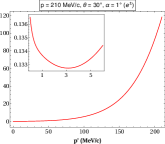
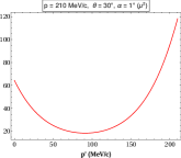
Figure 5: Behavior of the squared momentum transfer $-q^{2}$ (in units of $10^{2}$ MeV${}^{2}/c^{2}$), as a function of the outgoing lepton momentum, $p^{\prime}=|\vec{p}^{\,\prime}|$, for a fixed incident lepton momenta, $p=|\vec{p}\,|=210$ MeV/c, scattering angle, $\theta=30\degree$ and $\alpha=1\degree$. When $p^{\prime}\ll m_{e},|\vec{p}\,|$, we have near collinear photon emission with $\vec{p}$. In the case of electron scattering (left plot), the inset plot clearly displays the minimum of $-q^{2}$.

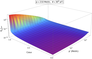
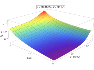
Figure 6: Behavior of $q^{-4}$ [in (MeV/c)^-4] as a simultaneous function of the outgoing lepton momenta $p^{\prime}$ and $0\leq\cos\alpha\leq 1$. The left plot is for the electron case and the right plot gives the muon results. In each case, the incident lepton momentum is $p=210$ MeV/c and the scattering angle is $\theta=30\degree$. In case of electron, there is a very large collinear enhancement for $p^{\prime}\to 0$ and $\alpha\to 0$ and manifests as a local maximum at small $p^{\prime}$ in Fig. 10. This phenomenon is not noticeable in the muon spectrum.

In Fig. 7, we display the result for the total differential cross section up to and including NLO in $\chi$PT, Eq. (LABEL:eq:sigma6), versus the cosine of the outgoing photon angle $\alpha$, for three MUSE specified incoming momenta, $p=|\vec{p}\,|=210,153,115$ MeV/c. For the bremsstrahlung process the outgoing lepton momentum can be chosen arbitrarily in the range $0\leq p^{\prime}\leq p^{\prime}_{elastic}(\theta)$, with $p_{elastic}(\theta)<p$ for a given scattering angle $\theta$. We only display the results for the MUSE specified kinematics with $p^{\prime}=30,100$ and $200$ MeV/c and for three forward angles: $\theta=15\degree,30\degree$ and $60\degree$. We also present a comparison of our NLO results with those of the LO (static and with recoil), as well as with the results obtained by using the corrected expression for Eq. (B.5) in Ref. motsai1969 (see clarification towards the end of this section). The differential cross section shows that the commonly used peaking approximation tsai1961 ; motsai1969 is very well satisfied for the electron even at these low electron momenta $p$ and $p^{\prime}$. The double-peak structure is a distinctive feature of the angular radiative spectrum for ultra-relativistic particles.

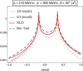
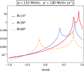
Figure 7: The bremsstrahlung differential cross section up to and including NLO in $\chi$PT, ${\rm d}^{3}\sigma/({\rm d}|\vec{p}^{\,\prime}|\,{\rm d}\Omega^{\prime}_{l}\,{\rm d}{\rm cos}\alpha)$ (in mb/GeV/sr), versus $\cos\alpha$ for electron scattering for the three incident MUSE specified momenta $p=|\vec{p}\,|$, as displayed. For each $p$ just one value for the outgoing electron momentum $p^{\prime}=|\vec{p}^{\,\prime}|$ is plotted. In the two l.h.s. and bottom right plots, the solid (red) curves correspond to $\theta=15\degree$, the dotted (blue) curves to $\theta=30\degree$, and the dashed (orange) curves to $\theta=60\degree$. The insert in the lower right graph shows the dominant $\zeta$-peak and the additional third peak very close to $\cos\alpha=1$. The top right graph compares the NLO result, Eq.(LABEL:eq:sigma6), with our LO evaluations, without [i.e., static, Eq. (21)], and with the proton recoil terms of ${\mathcal{O}}(m^{-1}_{p})$ in the phase space [i.e., recoil, Eq. (LABEL:eq:sigma5)]. In the same graph, the dashed curve shows the corresponding result obtained using the corrected expression for Eq. (B.5) in Ref. motsai1969 (see text).

The prominent double peaks occur for photon angle $\alpha$ close to the angle $\zeta$ (the $\zeta$-peak) for the incoming electron momentum, and the angle $\gamma$ (the $\gamma$-peak) for the outgoing electron momentum, as defined in Fig. 4. Moreover, it may be noted in the figure that for $\theta=15\degree$ for both the lower plots (as well as for $\theta=30\degree$ and $60\degree$ in the lower right plot) three peaks are generated with the $\zeta$-peak being the dominant one. In each case the rightmost peak-like structure very close to $\cos\alpha=1$, as shown by the insert plot in the lower right graph in Fig. 7, can be attributed to the small $q^{2}$ (or alternatively, large $1/q^{4}$) behavior for angle $\alpha$ close to zero (also, see Fig. 11 in Ref. motsai1969 ). As expected from a classical bremsstrahlung angular spectrum (see, e.g., Ref. motsai1969 ), for relativistic electrons the emitted photons get collimated close to the incoming and outgoing directions of the electron momentum. Several further observations regarding the electron plots are in order:

• The separation between the peaks increase with increasing scattering angle $\theta=\gamma-\zeta$. For $\theta\to 0$, the two peaks merge together into a single sharp peak, denoting collinear alignment of all momentum vectors.

• For a finite electron mass $m_{e}$, incident momentum $|\vec{p}\,|$, and fixed angles ($\theta,\alpha$), the differential cross section becomes maximum when the outgoing three-momentum $p^{\prime}$ value corresponding to the minimum of $-q^{2}$ (maximum of $1/q^{4}$).

• For fixed scattering angle $\theta$ and three-momentum transfer $|\vec{Q}|=|\vec{p}-\vec{p}^{\,\prime}|$, the differential cross section decreases with increasing incident momentum $|\vec{p}\,|$.

• For fixed three-momenta $p$ and $p^{\prime}$, the differential cross section decreases with increasing scattering angle $\theta$.

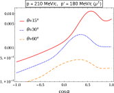
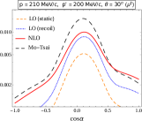
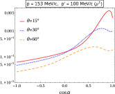
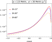
Figure 8: The bremsstrahlung differential cross section up to and including NLO in $\chi$PT, ${\rm d}^{3}\sigma/({\rm d}|\vec{p}^{\,\prime}|\,{\rm d}\Omega^{\prime}_{l}\,{\rm d}{\rm cos}\alpha)$ (in mb/GeV/sr) versus $\cos\alpha$ for muon scattering for the three incident MUSE specified momenta $p=|\vec{p}\,|$, as displayed. For each $p$ just one value for the outgoing muon momentum $p^{\prime}=|\vec{p}^{\,\prime}|$ is plotted. See text and caption of Fig. 7 for details.

In contrast to our electron scattering results, the $\cos\alpha$ dependence with the same kinematics for incoming muons is very different, as seen in Fig. 8. The initial muon momenta are not much larger than the muon mass, and the bremsstrahlung differential cross section versus $\cos\alpha$ has a broad angular spectrum. The plots in Figs. 7 and 8 clearly demonstrate that the so-called peaking approximations motsai1969 , a widely used practical recipe for data analysis incorporating radiative corrections, while viable for electron scattering at the low-momentum MUSE kinematics, is not applicable for muon scattering at MUSE energies. As seen from Fig. 7 (top right plot), the expressions for the NLO “interference” corrections, namely, Eqs. (23) - (LABEL:eq:sigma7), appear to yield contributions much smaller compared to the dominant LO result for the electron scattering. In contrast, for the muon scattering the NLO corrections are appreciably larger, as evidenced from the comparison plot in Fig. 8. Regarding our LO results, we have checked that the interference contribution in the LO differential bremsstrahlung cross section, Eq. (LABEL:eq:sigma5), is much larger and dominates over the “direct” contribution for both the electron and muon scattering (provided that the value for $p^{\prime}$ is not too small for the electron scattering case). As expected, the muon bremsstrahlung differential cross section is reduced by roughly two orders of magnitude compared to the corresponding electron cross sections for the same kinematic specification.

Zooming in on each peak in the electron angular $\cos\alpha$ dependence reveals the existence of a (3D) cone-like sub-structure, as displayed in Fig. 9, i.e., the photon emission is (almost) collinear with the incoming and outgoing electron momenta. It may be recalled that for a charged relativistic particle with an acceleration parallel to its velocity $\vec{\beta}$, the angular intensity distribution of the classical radiation corresponds to a cone with maximal opening angle $\sim{\mathcal{O}}(\sqrt{1-\beta^{2}})$ with respect to the direction of motion $\vec{\beta}$. The dashed vertical lines in Fig. 9 correspond in our reference system, Fig. 4, to the expected directions of the incoming and outgoing leptons. The effect of bremsstrahlung radiation results in the lepton recoiling away in a slightly different direction, leading to the characteristic cone-like feature for each peak with the vertex along the expected axis of the radiation cone. Unlike the $\cos\alpha$ dependence of the electron bremsstrahlung cross section, in case of the muon we observe significant interference effects between the two dominant broad angular peak structures arising entirely from the “direct” terms, labelled $[\dots]_{\rm dir(\gamma)}$ and $[\dots]_{\rm dir(\zeta)}$, and the “interference” contribution, labelled $[\dots]_{\rm int}$, in the LO expression Eq. (LABEL:eq:sigma5). We find in addition a nominal NLO correction Eq. (LABEL:eq:sigma7) to the $\cos\alpha$ behavior. These lead to the deviations of each minimum from the expected directions, as indicated by the vertically (red) dashed lines in the figure. Our graphic demonstrations support part of the analysis presented in Ref. ent01 (e.g., see, Fig. 4 in this reference), where radiative corrections to $(e,e^{\prime}p)$ coincident experiments were discussed. It is to be, however, noted that if we were to reduce the value of the muon mass from its physical value, there should be a steady reduction of this observed mismatch between the vertical (red) dashed lines and the cone minima.

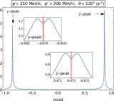
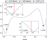
Figure 9: The bremsstrahlung differential cross sections up to and including NLO in $\chi$PT, ${\rm d}^{3}\sigma/({\rm d}|\vec{p}^{\,\prime}|\,{\rm d}\Omega^{\prime}_{l}\,{\rm d}{\rm cos}\alpha)$ (in mb/GeV/sr), versus $\cos\alpha$, indicating photon emissions from the leptons distributed within a shallow cone about their incident or scattered directions. The left plot is for electrons whereas the right plot is for muons. Both plots correspond to $p=210$ MeV/c and $p^{\prime}=200$ MeV/c, and for the lepton scattering angle $\theta=120\degree$. The red dashed lines indicate the directions of the incident and scattered leptons, i.e., $\cos\zeta$ and $\cos\gamma$, respectively.

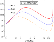
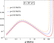
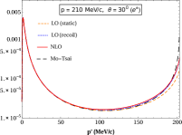
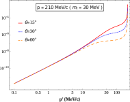
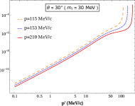
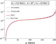
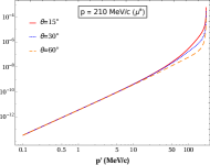
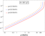
Figure 10: The “radiative tail spectrum” cross section up to and including NLO in $\chi$PT, ${\rm d}^{2}\sigma/({\rm d}|\vec{p}^{\,\prime}|\,{\rm d}\Omega^{\prime}_{l})$ (in mb/GeV/sr) is plotted as a function of the scattered lepton momentum $|\vec{p}^{\,\prime}|$, for incoming lepton momenta $|\vec{p}|$ and scattering angles $\theta$ specified by MUSE. The plots in the upper (lower) row correspond to electron (muon) scattering, while the plots in the middle row correspond to the results for an intermediate lepton mass, $m_{l}\sim 30$ MeV. In the left column plots, where $|\vec{p}\,|=210$ MeV/c, we display the cross sections for $\theta=15\degree$ solid (red) curve, 30$\degree$ dotted (blue) curve, and 60$\degree$ dashed (orange) curve. For the middle column plots, we show the cross sections with $\theta=30\degree$ for the three incoming MUSE specified momenta, $p=210$ (solid), $153$ (dotted) and $115$ (dashed) MeV/c in the static approximation $m_{p}\to\infty$. The right column plots (with non-log scale abscissa) compare our NLO results with the static and recoil LO evaluations, Eqs. (21) and (LABEL:eq:sigma5), respectively, as well as with the results obtained using the corrected expression for Eq. (B.5) in Ref. motsai1969 , but ignoring the proton form factors.

The NLO results for the electron and muon bremsstrahlung “radiative tail” cross section given in Eq. (LABEL:eq:sigma6) for the MUSE specified values of the incoming lepton momenta, i.e., $p=|\vec{p}\,|=210,153$ and $115$ MeV/c, are displayed in Figs. 10. We only display the plots for the forward scattering angles, $\theta=15\degree,30\degree$, and $60\degree$, also specified for MUSE measurements. The bremsstrahlung cross section versus $p^{\prime}$ is plotted from 0.1 MeV/c up to $p^{\prime}_{max}=p^{\prime}_{elastic}-\Delta p^{\prime}$, where we have chosen $\Delta p^{\prime}=0.1$ MeV/c in order to avoid the IR singular region. There is clearly a large IR enhancement of all the plots toward the large $p^{\prime}$ endpoint region. Without a proper treatment of the radiative IR divergences, our large $p^{\prime}$ results are beset with large uncertainties, though in the low-momentum region $p^{\prime}\lesssim 100$ MeV/c (suitable for MUSE) our results are reasonably accurate. We note that as $p^{\prime}$ tends toward zero, the differential cross section also goes to zero for the both muon and electron cases. However, for the electron tail spectrum the cross section reaches a local maximum before going to zero as $p^{\prime}\to 0$.

This local maximum at small $p^{\prime}$ values is primarily due to the dominant behavior of our static LO radiative tail cross section. When the outgoing electron momentum $\vec{p}^{\,\prime}\to 0$, the photon emission from the electron becomes (almost) collinear with the direction of the incident electron momentum $\vec{p}$ (reflected in the peaking approximation in Figs. 7 and 9) and the momentum transfer, $\vec{q}=\vec{p}-\vec{p}^{\,\prime}-\vec{k}$. If we artificially let the electron mass go towards zero, we will encounter a mass singularity when $p^{\prime}=0$. The small electron mass effectively regularizes this singularity, and a remnant of this divergence manifests itself as a local maximum in the cross section. In that case the cross section goes to zero as $p^{\prime}\to 0$.

Another way to examine the gradual development of the local maximum in the electron cross section is to consider our muon results presented in Fig. 10 (lower row plots) and artificially lower the value of the muon mass from the physical value, i.e., $m_{\mu}=105.7$ MeV. We find that for a lepton mass, $m_{l}\sim 30-40$ MeV, the cross section starts developing a “shoulder”, which for still smaller lepton mass values develops into a local maximum for small $p^{\prime}$ values. It then starts to resemble the cross section for electron scattering (upper row plots in Fig. 10). Thus, for sufficiently small values of the lepton mass, the cross section has a distinct local maximum in the cross section in the small $p^{\prime}$ region.

As evident from Fig. 10, our results up to and including the NLO appear to be dominated by the LO results. In other words, the qualitative difference made by the NLO corrections to the electron and the muon cross sections are not at all apparent from the figure. Thus, for a better qualitative estimate of the NLO part of tail spectrum, we present a relative comparison between the LO and NLO contributions in terms of a quantity, $\delta_{\rm NLO}$, which measures the ratio of the NLO correction with respect to the LO contribution, namely

$$\delta_{\rm NLO}=\left[\left(\frac{{\rm d}^{2}\sigma^{\rm(NLO)}}{{\rm d}p^{\prime}{\rm d}\Omega_{l}}\right)-\left(\frac{{\rm d}^{2}\sigma^{\rm(LO)}}{{\rm d}p^{\prime}{\rm d}\Omega_{l}}\right)\right]\text{\huge/}\left(\frac{{\rm d}^{2}\sigma^{\rm(LO)}}{{\rm d}p^{\prime}{\rm d}\Omega_{l}}\right)\,.$$ (26)

This quantity is plotted in Fig. 11 against the outgoing lepton momentum $p^{\prime}$, corresponding to the same kinematics specification as in the right column plots in Fig. 10. Clearly, the $\delta_{\rm NLO}$ for the muon spectrum is an order of magnitude larger than same for the electron spectrum. Moreover, in the electron case, the NLO corrections in the low $p^{\prime}$ region below 50 MeV/c become negative, in contrast to the NLO corrections for the muon that remain positive definite for the entire range of $p^{\prime}$ values.

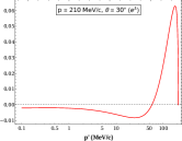
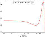
Figure 11: The quantity $\delta_{\rm NLO}$ of Eq. (26), which stands for the NLO corrections relative to LO radiative tail cross section, is plotted as a function of the outgoing lepton momentum $p^{\prime}<p^{\prime}_{elastic}$, where $p^{\prime}_{elastic}\approx 203.8$ MeV/c for electron and about $203.1$ MeV/c for muon, for scattering angle $\theta=30\degree$. The left plot is for the electron case and the right plot gives the corresponding muon results.

Finally, in comparing our results with the expression Eq. (B.5) in Ref. motsai1969 , we find that the expression has to be corrected as follows. The very first energy factor, $E_{p}/E_{s}$, multiplying the integral in that expression should have been $\vec{p}^{\,\,2}/(E_{p}E_{s})$. This reduces to the energy factor in Eq. (B.5) provided we neglect the lepton mass. Incorporating this correction and by ignoring the proton form factors (anomalous magnetic moment contribution also excluded) in Eq. (B.5) of Ref. motsai1969 , we find only a nominal difference with our LO result obtained from Eq. (LABEL:eq:sigma5). However, once we include the full NLO result obtained by evaluating Eqs. (LABEL:eq:sigma6) and (LABEL:eq:sigma7), which includes the $m_{p}^{-1}$ recoil corrections from the phase space, the $\delta$-function, and the matrix elements, the differences with Ref. motsai1969 indeed becomes negligible, as evident from the right column plots in Figs. 10. Note that Ref. motsai1969 treated both the leptons and the proton in a common relativistic framework, whereas in our $\chi$PT approach the proton, being a heavy particle, is treated non-relativistically in both the phase-space expressions and the matrix elements.

V Discussions and Summary

As mentioned in the introduction and in Sec. $\rm II$, the pion loops, as well as $m_{p}^{-2}$ terms from ${\cal L}_{\pi N}^{(2)}$ contribute at NNLO in $\chi$PT and generate the low-momentum proton form factors. These contributions are supposed to be small according to standard $\chi$PT counting. However, as presented in Sec. II the $\rm\chi PT$ counting scheme might not capture the fact that the probability of an electron radiating is much enhanced compared to the radiation from the heavy proton. Hence, we next examine the importance of the proton form factors generated by NNLO terms. The low-momentum NNLO expressions for the Sachs form factors $G^{p}_{E,M}$, have already been evaluated in earlier $\chi$PT works, e.g., Ref. Bernard1998 , and they are effectively incorporated in our evaluation. We consider only those LO Feynman graphs where the real photon radiation originates from one of the lepton lines, i.e., diagrams (A) and (B) in Fig. 1. We only include the dominant Sachs electric form factor $G^{p}_{E}$ of the proton, in particular the Taylor expanded form given by Eq. (9), at the exchanged photon-proton vertices associated with the LO diagrams. In order to have a rough assessment of the relative importance of the proton’s structure effects, we show our results as a ratio ${\mathscr{R}}$, which may be taken as a qualitative measure of the expected NNLO corrections $\delta_{\rm NNLO}$:

$${\mathscr{R}}=\frac{\left(\frac{{\rm d}^{2}\sigma}{{\rm d}p^{\prime}{\rm d}\Omega^{\prime}_{l}}\right)_{\rm form}\!\!\!-\,\left(\frac{{\rm d}^{2}\sigma}{{\rm d}p^{\prime}{\rm d}\Omega^{\prime}_{l}}\right)_{\rm point}}{\left(\frac{{\rm d}^{2}\sigma}{{\rm d}p^{\prime}{\rm d}\Omega^{\prime}_{l}}\right)_{\rm point}}\,.$$ (27)

Here, the subscripts “form” and “point”, respectively, denotes the radiative tail differential cross section evaluated with and without the proton’s r.m.s. charge radius $r^{p}_{E}$ included. Thus, in our analysis we approximate the NNLO $\chi$PT contributions as

$$\left(\frac{{\rm d}^{2}\sigma}{{\rm d}p^{\prime}\,{\rm d}\Omega^{\prime}_{l}}\right)_{\rm form}\!\!\!\! \to \int^{1}_{-1}{\rm d}(\cos\alpha)\left(\frac{{\rm d}^{3}\sigma^{\rm(LO)}}{{\rm d}p^{\prime}\,{\rm d}\Omega^{\prime}_{l}\,{\rm d}\cos\alpha}\right)G^{p}_{E}(q^{2})\,,$$

$$\left(\frac{{\rm d}^{2}\sigma}{{\rm d}p^{\prime}\,{\rm d}\Omega^{\prime}_{l}}\right)_{\rm point}\!\!\!\! \to \frac{{\rm d}^{2}\sigma^{\rm(LO)}}{{\rm d}p^{\prime}\,{\rm d}\Omega^{\prime}_{l}}\,,$$ (28)

with $q^{2}$ given by Eq. (14), and the charge radius $r^{p}_{E}$ of the proton to be used as the input. In phenomenological analyses, the dipole parametrization dipole is a commonly employed parametrization for the Sachs form factors, as was used in Ref. motsai1969 that correspond to $r^{p}_{E}=0.81$ fm. Furthermore, the recent high-precision measurements from the study of muonic hydrogen spectroscopy by the CREMA experimental collaboration pohl10 ; pohl13 led to the controversial value of $r^{p}_{E}=0.84$ fm, a result that is $\sim 7\sigma$ smaller than the previously accepted CODATA result, $r^{p}_{E}=0.87$ fm Mohr2012 . These three values of $r^{p}_{E}$ are used as the “measured” r.m.s. radius input to $G^{p}_{E}$ in the above relation. The results are displayed in Fig. 12 where they are labelled as “$\chi$PT (dople)”, “$\chi$PT (CREMA)” and “$\chi$PT (CODATA)”, respectively. Finally, these NNLO predictions are compared with the corresponding result obtained by using Eq. (B.5) of Ref. motsai1969 (with our corrected version), with and without their phenomenological electric form factor $G^{p}_{E}$ for obtaining the “form” and “point” contributions, respectively, while ignoring their magnetic dipole form factor $G^{p}_{M}$. This result is labelled as “Mo-Tsai” in the figure.

By comparing the plots in Figs. 11 and 12, we observe that the NLO and NNLO corrections relative to the LO results can be significant. As evident from the plots, for an incoming electron of momentum $p=210$ MeV/c, outgoing momentum $p^{\prime}=100$ MeV/c, and scattering angle $\theta=30\degree$, we find that the NLO and NNLO corrections modify the LO radiative tail cross section by about $2\%$ and $1\%$, respectively, with the “$\chi$PT” form factors [i.e., Eq. (9) with the above phenomenological r.m.s. radii.] Using the same kinematics for the muon, the corresponding LO results get modified about $20\%$ and $2\%$, respectively. In addition, our NNLO results suggest that effectively the pion loops strongly suppress the local maximum at small $p^{\prime}$ values in the electron radiative tail cross section. In case of the electron the crucial observation is that the NNLO form factor effects are of the same order as our NLO contributions. However, for the muon we find that the NNLO “$\chi$PT” contributions are about a factor of two smaller than the NLO contributions and more consistent with the standard $\chi$PT counting rules. But again in contrast, Fig.12 shows that for the muon “Mo -Tsai” result the proton’s structure contributions are a factors of two larger than those of the NNLO “$\chi$PT” results, and therefore, of similar magnitude as that of the muon NLO result shown in Fig. 11.

In Fig. 10, the bremsstrahlung cross sections diverge as the maximal value $p^{\prime}_{max}$ approaches the elastic lepton-proton scattering value $p^{\prime}_{elastic}$. As mentioned this is due to the infrared divergence (IR) of the bremsstrahlung process when the bremsstrahlung photon energy tends to zero. As demonstrated in, e.g., Refs. maximon00 ; motsai1969 , the cross section is free of IR singularities, provided the virtual radiative corrections are included in the calculation. In $\chi$PT, one can systematically evaluate the effect of virtual photon-loops, as well as the bremsstrahlung contribution from the leptons and protons in order to remove the IR singularities from observables. For the elastic lepton-proton scattering, the virtual photon loops along with the so-called two-photon exchange (TPE) contributions will additionally introduce ultraviolet (UV) divergences. These divergences can be treated systematically in $\chi$PT using the procedure of dimensional regularization which ensure gauge invariance at every perturbative order. To the best of our knowledge, such an evaluation has not been pursued to date in the context of low-energy lepton-proton scattering. This would naturally involve the introduction of low-energy constants (LECs) in the $\chi$PT Lagrangian required for the purpose of renormalization. Fortunately, at the order of our interest, all such LECs are known and can be taken directly from earlier $\chi$PT works, e.g., Ref. Ando . Such a systematic evaluation of the radiative corrections is beyond the scope of the present discussion, and shall be pursued in a future work.

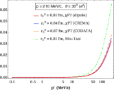
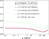
Figure 12: The quantity, $|\delta_{\rm NNLO}|$ is a qualitative measure of the expected NNLO proton’s r.m.s. radius contribution to the radiative tail cross section when the lepton is radiating. This quantity is plotted as a function of the outgoing lepton momentum $p^{\prime}<p^{\prime}_{elastic}$, where $p^{\prime}_{elastic}\approx 203.8$ MeV/c for electron and about $203.1$ MeV/c for muon, for scattering angle $\theta=30\degree$. Here different r.m.s. radii are used as phenomenological input to parametrize the “$\chi$PT” electric form factor $G^{p}_{E}$ (see text). For comparison, we also display the corresponding result obtained by using Eq. (B.5) of Ref. motsai1969 , while ignoring the magnetic form factor contribution. The left (right) plot corresponds to the electron (muon) results.

In retrospect, the purpose of this work was to present a qualitative but yet pedagogical evaluations of the LO and NLO contributions to the lepton-proton bremsstrahlung cross section in the context of a low-energy EFT framework. Here we summarize some of the essential aspects of this work:

• One important issue was to discuss a scenario where a large change in the angular spectrum of the bremsstrahlung process can be expected at typical momenta not much larger than the muon mass. The importance of such a study is very relevant to the MUSE experimental program where high precision lepton-proton scatterings at very low-momentum transfers will be pursued in order to investigate the reason behind the unexpectedly large discrepancy of the proton charge radius extracted from scattering experiments and the radius obtained from muonic hydrogen measurements. Our analysis demonstrates that a non-standard treatment of the bremsstrahlung corrections for muon scattering must be carefully thought through by the MUSE collaboration.

• In $\chi$PT employing Coulomb gauge, the two LO diagrams (C) and (D) in Fig.  1, and the two NLO diagrams, (I) and (J) in Fig. 2, do not contribute. In other words, bremsstrahlung radiation from a LO proton-photon vertex does not contribute in our $\chi$PT analysis. However, there is non-trivial proton bremsstrahlung contributions [diagrams (G) and (H) in Fig. 2] at NLO associated with chiral order $\nu=1$ proton-photon vertex in $\chi$PT.

• While taking the trace over the amplitude squared in order to determine the unpolarized bremsstrahlung cross section, the spin dependent interactions in the NLO Lagrangian give vanishing contribution. Consequently, the anomalous magnetic moment of the proton does not contribute to the cross section for this process at NLO in $\chi$PT, contrary to usual expectations. Thus, the proton’s magnetic moment starts contributing to the bremsstrahlung process only at NNLO, as implicitly parametrized in our case in terms of the proton’s r.m.s. radius.

• Our results displayed in Figs. 7 and 8, clearly indicate that the widely used peaking approximation in radiative analysis of high energy electron scattering data can not be used in the radiative analyses of the future low-energy muon data from MUSE.

• As evidenced from Fig. 10, the radiative tail cross section for the electron scattering process for small outgoing momenta, $p^{\prime}\lesssim 5$ MeV/c exhibits a local maximum that can be attributed due to the small but non-zero electron mass. However, in the same figure we show that such a behavior disappears for the much larger lepton muon mass. Since MUSE is designed only to detect the lepton scattering angle $\theta$ and can not determine the value of the outgoing lepton momentum $|\vec{p}^{\,\prime}\,|$, care must be taken in the analysis of the MUSE data when one corrects for the radiative tail from the bremsstrahlung spectra.

• At NNLO the proton’s r.m.s. radius enters the evaluation via the LECs in ${\cal L}_{\pi N}^{(2)}$, meaning that the low-momentum aspects of the proton’s structure (r.m.s. radius) naturally contribute at this sub-leading order. In particular, we find that NNLO corrections for electron scattering bremsstrahlung diagrams illustrated in Fig. 3, are as large as the NLO corrections, contrary to what is expected in standard chiral power counting.

• Finally, we report that our evaluations revealed a misprint in the overall energy factor in the well-known review article motsai1969 .

As a future extension of this work, we intend to improve on the systematic uncertainties and evaluate the radiative corrections to the lepton-proton bremsstrahlung scattering process (including the two-photon exchange corrections) which should eliminate the unphysical IR singularities in the large $p^{\prime}$ region in all the differential cross sections considered in this work.

VI Acknowledgments

Numerous discussions with Steffen Strauch have been very helpful in the present work. We thank Ulf Meißner, Daniel Phillips and Shung-Ichi Ando for useful comments. One of us (FM) is grateful for the hospitality at Ruhr University Bochum while working on this project.

Appendix A The partial NLO amplitudes in Eq. (LABEL:eq:sigma7)

We display the eight partial amplitudes appearing in our NLO corrections to the lepton-proton bremsstrahlung differential cross section, Eq. (LABEL:eq:sigma7), namely

$$W_{AE} = -\,m_{l}^{2}E_{l}(\vec{p}_{p}^{\,\prime}\cdot\vec{p}^{\,\prime})-m_{l}^{2}E_{l}(\vec{p}_{p}\cdot\vec{p}^{\,\prime})+m_{l}^{2}E^{\prime}_{l}(\vec{p}_{p}^{\,\prime}\cdot\vec{k})+m_{l}^{2}E^{\prime}_{l}(\vec{p}_{p}\cdot\vec{k})-m_{l}^{2}E^{\prime}_{l}(\vec{p}_{p}^{\,\prime}\cdot\vec{p})-m_{l}^{2}E^{\prime}_{l}(\vec{p}_{p}\cdot\vec{p})+m_{l}^{2}E^{0}_{\gamma}(\vec{p}_{p}^{\,\prime}\cdot\vec{p}^{\,\prime})$$

$$+\,m_{l}^{2}E^{0}_{\gamma}(\vec{p}_{p}\cdot\vec{p}^{\,\prime})+E_{l}(E^{0}_{\gamma})^{2}(\vec{p}_{p}\cdot\vec{p}^{\,\prime})+E_{l}(E^{0}_{\gamma})^{2}(\vec{p}_{p}^{\,\prime}\cdot\vec{p}^{\,\prime})+E_{l}E^{\prime}_{l}E^{0}_{\gamma}(\vec{p}_{p}\cdot\vec{k})+E_{l}E^{\prime}_{l}E^{0}_{\gamma}(\vec{p}_{p}^{\,\prime}\cdot\vec{k})-E^{\prime}_{l}(\vec{p}_{p}^{\,\prime}\cdot\vec{k})(\vec{p}\cdot\vec{k})$$

$$-\,E^{\prime}_{l}(\vec{p}_{p}\cdot\vec{k})(\vec{p}\cdot\vec{k})-E^{0}_{\gamma}(\vec{p}_{p}^{\,\prime}\cdot\vec{p}^{\,\prime})(\vec{p}\cdot\vec{k})-E^{0}_{\gamma}(\vec{p}_{p}\cdot\vec{p}^{\,\prime})(\vec{p}\cdot\vec{k})\,,$$

$$W_{AF} = m_{l}^{2}E_{l}(\vec{p}_{p}^{\,\prime}\cdot\vec{k})+m_{l}^{2}E_{l}(\vec{p}_{p}\cdot\vec{k})+m_{l}^{2}E^{\prime}_{l}(\vec{p}_{p}^{\,\prime}\cdot\vec{k})+m_{l}^{2}E^{\prime}_{l}(\vec{p}_{p}\cdot\vec{k})+m_{l}^{2}E^{0}_{\gamma}(\vec{p}_{p}^{\,\prime}\cdot\vec{k})+m_{l}^{2}E^{0}_{\gamma}(\vec{p}_{p}\cdot\vec{p})+m_{l}^{2}E^{0}_{\gamma}(\vec{p}_{p}\cdot\vec{p}^{\,\prime})$$

$$+\,m_{l}^{2}E^{0}_{\gamma}(\vec{p}_{p}\cdot\vec{k})-m_{l}^{2}E^{0}_{\gamma}(\vec{p}_{p}^{\,\prime}\cdot\vec{p}^{\,\prime})-m_{l}^{2}E^{0}_{\gamma}(\vec{p}_{p}^{\,\prime}\cdot\vec{p})+E_{l}^{2}E^{\prime}_{l}(\vec{p}_{p}^{\,\prime}\cdot\vec{p}^{\,\prime})+E_{l}^{2}E^{\prime}_{l}(\vec{p}_{p}\cdot\vec{p}^{\,\prime})+E_{l}^{2}E^{0}_{\gamma}(\vec{p}_{p}^{\,\prime}\cdot\vec{p}^{\,\prime})$$

$$+\,E_{l}^{2}E^{0}_{\gamma}(\vec{p}_{p}\cdot\vec{p}^{\,\prime})+E_{l}(E^{\prime}_{l})^{2}(\vec{p}_{p}^{\,\prime}\cdot\vec{p})+E_{l}(E^{\prime}_{l})^{2}(\vec{p}_{p}\cdot\vec{p})-E_{l}(E^{\prime}_{l})^{2}(\vec{p}_{p}^{\,\prime}\cdot\vec{k})-E_{l}(E^{\prime}_{l})^{2}(\vec{p}_{p}\cdot\vec{k})+E_{l}(\vec{p}_{p}^{\,\prime}\cdot\vec{p})(\vec{p}^{\,\prime}\cdot\vec{k})$$

$$+\,E_{l}(\vec{p}_{p}^{\,\prime}\cdot\vec{p}^{\,\prime})(\vec{p}^{\,\prime}\cdot\vec{k})+E_{l}(\vec{p}_{p}\cdot\vec{p})(\vec{p}^{\,\prime}\cdot\vec{k})+E_{l}(\vec{p}_{p}\cdot\vec{p}^{\,\prime})(\vec{p}^{\,\prime}\cdot\vec{k})-E_{l}(\vec{p}_{p}^{\,\prime}\cdot\vec{p}^{\,\prime})(\vec{p}\cdot\vec{p}^{\,\prime})-E_{l}(\vec{p}_{p}^{\,\prime}\cdot\vec{p}^{\,\prime})(\vec{p}\cdot\vec{k})$$

$$-\,E_{l}(\vec{p}_{p}\cdot\vec{p}^{\,\prime})(\vec{p}\cdot\vec{p}^{\,\prime})-E_{l}(\vec{p}_{p}\cdot\vec{p}^{\,\prime})(\vec{p}\cdot\vec{k})+E^{\prime}_{l}(\vec{p}_{p}^{\,\prime}\cdot\vec{k})(\vec{p}\cdot\vec{p}^{\,\prime})+E^{\prime}_{l}(\vec{p}_{p}\cdot\vec{k})(\vec{p}\cdot\vec{p}^{\,\prime})-E^{\prime}_{l}(\vec{p}_{p}\cdot\vec{p})(\vec{p}\cdot\vec{p}^{\,\prime})$$

$$-\,E^{\prime}_{l}(\vec{p}_{p}\cdot\vec{p}^{\,\prime})(\vec{p}\cdot\vec{k})-E^{\prime}_{l}(\vec{p}_{p}^{\,\prime}\cdot\vec{p})(\vec{p}\cdot\vec{p}^{\,\prime})-E^{\prime}_{l}(\vec{p}_{p}^{\,\prime}\cdot\vec{p}^{\,\prime})(\vec{p}\cdot\vec{k})-E^{0}_{\gamma}(\vec{p}_{p}^{\,\prime}\cdot\vec{p})(\vec{p}\cdot\vec{p}^{\,\prime})+E^{0}_{\gamma}(\vec{p}_{p}\cdot\vec{p})(\vec{p}\cdot\vec{p}^{\,\prime})\,,$$

$$W_{AG} = m_{l}^{2}E_{l}^{2}E^{0}_{\gamma}+E_{l}^{3}E^{\prime}_{l}E^{0}_{\gamma}+2m_{l}^{2}E_{l}(\vec{p}_{p}\cdot\vec{p})-m_{l}^{2}E_{l}(\vec{p}_{p}\cdot\vec{k})-m_{l}^{2}E_{l}(\vec{p}\cdot\vec{k})+2E_{l}^{2}E^{\prime}_{l}(\vec{p}_{p}\cdot\vec{p})-E_{l}^{2}E^{\prime}_{l}(\vec{p}_{p}\cdot\vec{k})$$

$$-\,E_{l}^{2}E^{\prime}_{l}(\vec{p}\cdot\vec{k})-E^{\prime}_{l}E_{l}E^{0}_{\gamma}(\vec{p}_{p}\cdot\vec{p})+E_{l}^{2}E^{0}_{\gamma}(\vec{p}\cdot\vec{p}^{\,\prime})-E_{l}^{2}E^{0}_{\gamma}(\vec{p}_{p}\cdot\vec{p}^{\,\prime})+2E_{l}(\vec{p}_{p}\cdot\vec{p})(\vec{p}\cdot\vec{p}^{\,\prime})-E_{l}(\vec{p}_{p}\cdot\vec{p})(\vec{p}^{\,\prime}\cdot\vec{k})$$

$$+\,E_{l}(\vec{p}_{p}\cdot\vec{p}^{\,\prime})(\vec{p}\cdot\vec{k})-E_{l}(\vec{p}_{p}\cdot\vec{k})(\vec{p}\cdot\vec{p}^{\,\prime})-E_{l}(\vec{p}\cdot\vec{p}^{\,\prime})(\vec{p}\cdot\vec{k})\,,$$

$$W_{AH} = m_{l}^{2}E_{l}^{2}E^{0}_{\gamma}+E_{l}^{3}E_{l}^{\prime}E^{0}_{\gamma}+m_{l}^{2}E_{l}(\vec{p}_{p}^{\,\prime}\cdot\vec{k})-2m_{l}^{2}E_{l}(\vec{p}_{p}^{\,\prime}\cdot\vec{p})-m_{l}^{2}E_{l}(\vec{p}\cdot\vec{k})-2E_{l}^{2}E^{\prime}_{l}(\vec{p}_{p}^{\,\prime}\cdot\vec{p})+E_{l}^{2}E^{\prime}_{l}(\vec{p}_{p}^{\,\prime}\cdot\vec{k})$$

$$+\,E^{\prime}_{l}E_{l}E^{0}_{\gamma}(\vec{p}_{p}^{\,\prime}\cdot\vec{p})-E_{l}^{2}E^{\prime}_{l}(\vec{p}\cdot\vec{k})+E_{l}^{2}E^{0}_{\gamma}(\vec{p}_{p}^{\,\prime}\cdot\vec{p}^{\,\prime})+E_{l}^{2}E^{0}_{\gamma}(\vec{p}\cdot\vec{p}^{\,\prime})+E_{l}(\vec{p}_{p}^{\,\prime}\cdot\vec{p})(\vec{p}^{\,\prime}\cdot\vec{k})-2E_{l}(\vec{p}_{p}^{\,\prime}\cdot\vec{p})(\vec{p}^{\,\prime}\cdot\vec{p})$$

$$+\,E_{l}(\vec{p}_{p}^{\,\prime}\cdot\vec{k})(\vec{p}^{\,\prime}\cdot\vec{p})-E_{l}(\vec{p}_{p}^{\,\prime}\cdot\vec{p}^{\,\prime})(\vec{p}\cdot\vec{k})-E_{l}(\vec{p}^{\,\prime}\cdot\vec{p})(\vec{p}\cdot\vec{k})\,.$$

$$W_{BE} = -\,m_{l}^{2}E_{l}(\vec{p}_{p}\cdot\vec{k})-m_{l}^{2}E_{l}(\vec{p}_{p}^{\,\prime}\cdot\vec{k})-m_{l}^{2}E_{l}^{\prime}(\vec{p}_{p}^{\,\prime}\cdot\vec{k})-m_{l}^{2}E_{l}^{\prime}(\vec{p}_{p}\cdot\vec{k})+m_{l}^{2}E^{0}_{\gamma}(\vec{p}_{p}\cdot\vec{p}^{\,\prime})+m_{l}^{2}E^{0}_{\gamma}(\vec{p}_{p}^{\,\prime}\cdot\vec{p}^{\,\prime})+m_{l}^{2}E^{0}_{\gamma}(\vec{p}_{p}\cdot\vec{p})$$

$$-\,m_{l}^{2}E^{0}_{\gamma}(\vec{p}_{p}^{\,\prime}\cdot\vec{k})-m_{l}^{2}E^{0}_{\gamma}(\vec{p}_{p}^{\,\prime}\cdot\vec{p})-m_{l}^{2}E^{0}_{\gamma}(\vec{p}_{p}\cdot\vec{k})+E_{l}^{2}E^{\prime}_{l}(\vec{p}_{p}^{\,\prime}\cdot\vec{p}^{\,\prime})+E_{l}^{2}E^{\prime}_{l}(\vec{p}_{p}\cdot\vec{p}^{\,\prime})+E_{l}^{2}E^{\prime}_{l}(\vec{p}_{p}\cdot\vec{k})+E_{l}^{2}E^{\prime}_{l}(\vec{p}_{p}^{\,\prime}\cdot\vec{k})$$

$$+\,E_{l}(E_{l}^{\prime})^{2}(\vec{p}_{p}^{\,\prime}\cdot\vec{p})+E_{l}(E_{l}^{\prime})^{2}(\vec{p}_{p}\cdot\vec{p})-(E_{l}^{\prime})^{2}E^{0}_{\gamma}(\vec{p}_{p}^{\,\prime}\cdot\vec{p})-(E_{l}^{\prime})^{2}E^{0}_{\gamma}(\vec{p}_{p}\cdot\vec{p})+E_{l}(\vec{p}_{p}^{\,\prime}\cdot\vec{p})(\vec{p}^{\,\prime}\cdot\vec{k})+E_{l}(\vec{p}_{p}\cdot\vec{p})(\vec{p}^{\,\prime}\cdot\vec{k})$$

$$-\,E_{l}(\vec{p}_{p}\cdot\vec{k})(\vec{p}\cdot\vec{p}^{\,\prime})-E_{l}(\vec{p}_{p}^{\,\prime}\cdot\vec{p}^{\,\prime})(\vec{p}^{\,\prime}\cdot\vec{p})-E_{l}(\vec{p}_{p}^{\,\prime}\cdot\vec{k})(\vec{p}^{\,\prime}\cdot\vec{p})-E_{l}(\vec{p}_{p}\cdot\vec{p}^{\,\prime})(\vec{p}^{\,\prime}\cdot\vec{p})+E_{l}^{\prime}(\vec{p}_{p}^{\,\prime}\cdot\vec{p})(\vec{p}^{\,\prime}\cdot\vec{k})$$

$$+\,E_{l}^{\prime}(\vec{p}_{p}\cdot\vec{p})(\vec{p}^{\,\prime}\cdot\vec{k})-E_{l}^{\prime}(\vec{p}_{p}^{\,\prime}\cdot\vec{p})(\vec{p}^{\,\prime}\cdot\vec{p})-E_{l}^{\prime}(\vec{p}_{p}^{\,\prime}\cdot\vec{p})(\vec{p}\cdot\vec{k})-E_{l}^{\prime}(\vec{p}_{p}^{\,\prime}\cdot\vec{p}^{\,\prime})(\vec{p}\cdot\vec{k})-E_{l}^{\prime}(\vec{p}_{p}\cdot\vec{p})(\vec{p}\cdot\vec{p}^{\,\prime})$$

$$-\,E_{l}^{\prime}(\vec{p}_{p}\cdot\vec{p})(\vec{p}\cdot\vec{k})-E_{l}^{\prime}(\vec{p}_{p}\cdot\vec{p}^{\,\prime})(\vec{p}\cdot\vec{k})+E^{0}_{\gamma}(\vec{p}_{p}^{\,\prime}\cdot\vec{p}^{\,\prime})(\vec{p}\cdot\vec{p}^{\,\prime})+E^{0}_{\gamma}(\vec{p}_{p}\cdot\vec{p}^{\,\prime})(\vec{p}\cdot\vec{p}^{\,\prime})\,,$$

$$W_{BF} = -\,m_{l}^{2}E_{l}(\vec{p}_{p}^{\,\prime}\cdot\vec{p}^{\,\prime})-m_{l}^{2}E_{l}(\vec{p}_{p}\cdot\vec{p}^{\,\prime})-m_{l}^{2}E_{l}(\vec{p}_{p}^{\,\prime}\cdot\vec{k})-m_{l}^{2}E_{l}(\vec{p}_{p}\cdot\vec{k})-m_{l}^{2}E_{l}^{\prime}(\vec{p}_{p}^{\,\prime}\cdot\vec{p})-m_{l}^{2}E_{l}^{\prime}(\vec{p}_{p}\cdot\vec{p})-m_{l}^{2}E^{0}_{\gamma}(\vec{p}_{p}^{\,\prime}\cdot\vec{p})$$

$$-m_{l}^{2}E^{0}_{\gamma}(\vec{p}_{p}\cdot\vec{p})+\,E_{l}^{\prime}(E^{0}_{\gamma})^{2}(\vec{p}_{p}^{\,\prime}\cdot\vec{p})+E_{l}^{\prime}(E^{0}_{\gamma})^{2}(\vec{p}_{p}\cdot\vec{p})+E_{l}E_{l}^{\prime}E^{0}_{\gamma}(\vec{p}_{p}^{\,\prime}\cdot\vec{k})+E_{l}E_{l}^{\prime}E^{0}_{\gamma}(\vec{p}_{p}\cdot\vec{k})-E_{l}(\vec{p}_{p}^{\,\prime}\cdot\vec{k})(\vec{p}^{\,\prime}\cdot\vec{k})$$

$$-E_{l}(\vec{p}_{p}\cdot\vec{k})(\vec{p}^{\,\prime}\cdot\vec{k})-E^{0}_{\gamma}(\vec{p}_{p}^{\,\prime}\cdot\vec{p})(\vec{p}^{\,\prime}\cdot\vec{k})-E^{0}_{\gamma}(\vec{p}_{p}\cdot\vec{p})(\vec{p}^{\,\prime}\cdot\vec{k})\,,$$

$$W_{BG} = m_{l}^{2}(E_{l}^{\prime})^{2}E^{0}_{\gamma}+E_{l}E^{0}_{\gamma}(E_{l}^{\prime})^{3}+2m_{l}^{2}E_{l}^{\prime}(\vec{p}_{p}\cdot\vec{p}^{\,\prime})+m_{l}^{2}E_{l}^{\prime}(\vec{p}_{p}\cdot\vec{k})-m_{l}^{2}E_{l}^{\prime}(\vec{p}^{\,\,\prime}\cdot\vec{k})+2E_{l}(E_{l}^{\prime})^{2}(\vec{p}_{p}\cdot\vec{p}^{\,\prime})+E_{l}(E_{l}^{\prime})^{2}(\vec{p}_{p}\cdot\vec{k})$$

$$-\,E_{l}(E_{l}^{\prime})^{2}(\vec{p}^{\,\prime}\cdot\vec{k})+E_{l}E_{l}^{\prime}E^{0}_{\gamma}(\vec{p}_{p}\cdot\vec{p}^{\,\prime})+(E_{l}^{\prime})^{2}E^{0}_{\gamma}(\vec{p}_{p}\cdot\vec{p})+(E_{l}^{\prime})^{2}E^{0}_{\gamma}(\vec{p}^{\,\prime}\cdot\vec{p})+2E_{l}^{\prime}(\vec{p}_{p}\cdot\vec{p}^{\,\prime})(\vec{p}^{\,\prime}\cdot\vec{p})+E_{l}^{\prime}(\vec{p}_{p}\cdot\vec{k})(\vec{p}\cdot\vec{p}^{\,\prime})$$

$$+\,E_{l}^{\prime}(\vec{p}_{p}\cdot\vec{p}^{\,\prime})(\vec{p}\cdot\vec{k})-E_{l}^{\prime}(\vec{p}^{\,\prime}\cdot\vec{k})(\vec{p}^{\,\prime}\cdot\vec{p})-E_{l}^{\prime}(\vec{p}_{p}\cdot\vec{p})(\vec{p}^{\,\prime}\cdot\vec{k})\,,$$

$$W_{BH} = -\,m_{l}^{2}(E_{l}^{\prime})^{2}E^{0}_{\gamma}-E_{l}(E_{l}^{\prime})^{3}E^{0}_{\gamma}+m_{l}^{2}E_{l}^{\prime}(\vec{p}_{p}^{\,\prime}\cdot\vec{k})+m_{l}^{2}E_{l}^{\prime}(\vec{p}^{\,\prime}\cdot\vec{k})+2m_{l}^{2}E_{l}^{\prime}(\vec{p}_{p}^{\,\prime}\cdot\vec{p}^{\,\prime})+2E_{l}(E_{l}^{\prime})^{2}(\vec{p}_{p}^{\,\prime}\cdot\vec{p}^{\,\prime})+E^{2}_{l}(E_{l}^{\prime})^{2}(\vec{p}_{p}^{\,\prime}\cdot\vec{k})$$

$$+\,E_{l}(E_{l}^{\prime})^{2}(\vec{p}^{\,\prime}\cdot\vec{k})+E_{l}E_{l}^{\prime}E^{0}_{\gamma}(\vec{p}_{p}^{\,\prime}\cdot\vec{p}^{\,\prime})+(E_{l}^{\prime})^{2}E^{0}_{\gamma}(\vec{p}_{p}^{\,\prime}\cdot\vec{p})-(E_{l}^{\prime})^{2}E^{0}_{\gamma}(\vec{p}^{\,\prime}\cdot\vec{p})+2E_{l}^{\prime}(\vec{p}_{p}^{\,\prime}\cdot\vec{p}^{\,\prime})(\vec{p}^{\,\prime}\cdot\vec{p})+E_{l}^{\prime}(\vec{p}_{p}^{\,\prime}\cdot\vec{p}^{\,\prime})(\vec{p}\cdot\vec{k})$$

$$+\,E_{l}^{\prime}(\vec{p}_{p}^{\,\prime}\cdot\vec{k})(\vec{p}^{\,\prime}\cdot\vec{p})+E_{l}^{\prime}(\vec{p}^{\,\prime}\cdot\vec{k})(\vec{p}^{\,\prime}\cdot\vec{p})-E_{l}^{\prime}(\vec{p}_{p}^{\,\prime}\cdot\vec{p})(\vec{p}^{\,\prime}\cdot\vec{k})\,.$$

In the rest frame of hadron target, the three-momentum of the proton, $|\vec{p}\,|=0$. The expressions for the dot-products in our preferred frame of reference, Fig. 4, are:

$$\vec{p}\cdot\vec{p}^{\,\prime} = |\vec{p}^{\,\prime}||\vec{p}\,|\cos\theta\,,$$

$$\vec{k}\cdot\vec{p}^{\,\prime} = E_{\gamma}|\vec{p}^{\,\prime}|(\cos\gamma\,\cos\alpha+\sin\alpha\,\sin\gamma\,\cos\phi_{\gamma})\,,$$

$$\vec{k}\cdot\vec{p} = E_{\gamma}|\vec{p}\,|(\cos\zeta\,\cos\alpha+\sin\alpha\,\sin\zeta\,\cos\phi_{\gamma})\,,$$

$$\vec{p}_{p}^{\,\prime}\cdot\vec{p}^{\,\prime} = (\vec{Q}-\vec{k})\cdot\vec{p}^{\,\prime}=|\vec{Q}||\vec{p}^{\,\prime}|\cos\gamma-\vec{k}\cdot\vec{p}^{\,\prime}\,,$$

$$\vec{p}_{p}^{\,\prime}\cdot\vec{p} = (\vec{Q}-\vec{k})\cdot\vec{p}=|\vec{Q}||\vec{p}\,|\cos\zeta-\vec{k}\cdot\vec{p}\,,$$

$$\vec{p}_{p}^{\,\prime}\cdot\vec{k} = (\vec{Q}-\vec{k})\cdot\vec{k}=|\vec{Q}|E_{\gamma}\cos\alpha-E_{\gamma}^{2}\,.$$ (30)

References

- (1) R. Pohl, et al., Nature 466 (2010) 213.
- (2) P. J. Mohr, B. N. Taylor, and D. B. Newell, Rev. Mod. Phys. 84, 1527 (2012).
- (3) R. Pohl, R. Gilman, G. A. Miller, G. A. Nille, and K. Pachucki, Annu. Rev. Nucl. Part. Science, 63, 175 (2013).
- (4) J. Bernauer et al. (A1 Collaboration), Phys. Rev. Lett. 105, 242001 (2010).
- (5) X. Zhan et al., Phys. Lett. B 705, 59 (2011).
- (6) M. Mihovilovič et al., Phys. Lett. B 771, 194 (2017).
- (7) M. A. Belushkin, H.-W. Hammer and Ulf-G. Meissner, Phys. Rev. C 75, 035202 (2007).
- (8) I. T. Lorenz, H.-W. Hammer and U.-G. Meissner, Eur. Phys. J. A 48, 151 (2012).
- (9) R. Gilman, et al., Technical Design Report for the Paul Scherrer Institute Experiment R-12-01.1: Studying the Proton ”Radius” Puzzle with Elastic Scattering, arXiv:1709.09753
- (10) Lin Li, S. Strauch Personal communications.
- (11) L. Maximon, Rev. Mod. Phys. 41 193 (1969).
- (12) L. Maximon and J. Tjon, Phys. Rev. C 62, 054320 (2000).
- (13) Y.-S. Tsai, Phys. Rev. 122, 1898 (1961).
- (14) L. W. Mo and Y.-S. Tsai, Rev. Mod. Phys. 41 205 (1969).
- (15) V. Bernard, N. Kaiser and Ulf-G. Meißner, Int. J. Mod. Phys. Rev. E 4, (1995) 193.
- (16) R. Ent, et al., Phys. Rev. C 64, 054610 (2001).
- (17) J. D. Bjorken and S. D. Drell, “Relativistic Quantum Fields”, McGraw-Hill Book Comp., N.Y., 1965.
- (18) N. Fettes, Ph.D Dissertation, Univ. Bonn (2000), unpublished.
- (19) T. R. Hemmert, B. R. Holstein and J. Kambor, J. Phys. G 24 (1998) 1831.
- (20) G. Ecker, Phys. Lett. B 336 (1994) 508.
- (21) V Bernard, H. W. Fearing, T. R. Hemmert and Ulf-G. Meißner, Nucl. Phys. A 635 (1998) 121-145.
- (22) V. Bernard, N. Kaiser, J. Kambor and Ulf-G. Meißner, Nucl. Phys. B 388, 315 (1992).
- (23) A. V. Manohar and M. Luke, Phys. Lett. B 286, 348 (1992).
- (24) S. Ando et al., Phys. Lett. B 595, 250 (2004).
- (25) J. R. Dunning, et Phys. Rev. 141, 1286 (1966).