Comparison of U-net-based Convolutional Neural Networks for Liver Segmentation in CT

Abstract

Various approaches for liver segmentation in CT have been proposed: Besides statistical shape models, which played a major role in this research area, novel approaches on the basis of convolutional neural networks have been introduced recently. Using a set of 219 liver CT datasets with reference segmentations from liver surgery planning, we evaluate the performance of several neural network classifiers based on 2D and 3D U-net architectures.

An interesting observation is that slice-wise approaches perform surprisingly well, with mean and median Dice coefficients above 0.97, and may be preferable over 3D approaches given current hardware and software limitations.

1 Introduction

Liver segmentation has long been investigated, as it plays an important role when planning surgeries or catheter-based interventions [1, 2, 3]. Several clinical workflows require a volumetric analysis of the liver. The size and complex shape of the organ make manual delineation very time-consuming. On the other hand, its appearance in computed tomography scans varies a lot, for instance, when it contains hypo- or hyperdense tumors, necrosis, calcifications, cirrhosis, cysts, or contrast agent. Furthermore, several adjacent structures (e.g., heart, stomach, intestines) may have very similar appearance, causing low boundary contrast.

Proposed methods for liver segmentation range from semi-interactive [4] to fully automatic [5, 6, 7, 8, 9], and one of the first "challenges" organized for a fair and reproducible comparison of segmentation methods in medical image computing was on liver segmentation [3]. Many successful approaches employed statistical shape models as a representation of typical liver shapes for guiding the segmentation in the presence of the above difficulties [6, 5, 7]. More recently, convolutional neural networks (CNN) have received a lot of attention due to their ability to solve segmentation problems formulated as voxel classification tasks with sometimes impressive performance. Fully-convolutional network architectures (FCN) became very popular, because they allow for very efficient training and classification on many voxels at once [10]. In particular, so-called "U-nets" were proposed as a deep segmentation architecture supporting efficient end-to-end training of a multi-resolution model in 2D [11] and 3D [12, 13]. Other methods create the multi-resolution representation in the external preprocessing pipeline, feeding parallel low- and high-resolution streams into the neural network, which saves GPU memory and thus allows for larger training batches [14]. For liver segmentation, 2D U-nets were applied slice-wise, optionally combined with 3D conditional random fields [8]. Other authors applied a simple 3D CNN architecture to this task [9], with fewer layers, larger kernels, and smaller numbers of convolutional filters. An interesting compromise using three orthogonal 2D CNNs was proposed for cartilage segmentation in MRI [15].

The goal of this work was to quantitatively and qualitatively compare the performance of different U-net-based neural network architectures. Our evaluation includes various existing 2D and 3D variants of U-nets, and a novel approach using an ensemble of fully convolutional slice-wise classifiers operating on different view directions.

2 Methods

CT Datasets

We evaluated our method on a dataset comprising 219 liver CT volumes for surgery planning, acquired on different scanners with a resolution of about 0.6 mm in-plane and a reconstructed slice thickness of 0.8 mm. Iodinated contrast agent was applied in all cases. The data included healthy livers, organs with benign and/or malignant liver lesion, and pre-resected cases. Liver Segmentation and further planning was performed on the venous phase for two types of surgery: living donor liver transplantation [16], $n=52$, 24% and liver resection [2], $n=167$, 76%. Patient age ranged from 10-85 years (IQR 55-72) and 133 of the patients were male, 81 female. All cases were carefully annotated using a slice-wise approach based on live-wire, shape-based interpolation and interactive contour correction [4] and were reviewed by radiological experts.

After import, the DICOM rescale parameters were applied to get 16 bit Hounsfield integer values for the network’s input layer. Subsequently, for models using a fixed voxel size (2 mm or 1 mm, depending on the experiment), we rescaled the volumes to an isotropic voxel size with a Lanczos window for the CT data and a nearest neighbor interpolator for the corresponding binary mask.

Training vs. Test Sets

All available cases were randomly assigned to three disjunct groups for training, validation, and testing. The training cases were the largest group (comprising two thirds of the cases) and were directly used for deriving our models. Separate validation cases were used for evaluating performance during training. The test cases were not used for either of these, maximizing the likelihood of being able to predict generalization performance.

Neural Network Architectures

Figure 1: Overview of U-net architecture variant with four resolution levels (2D)

All neural network architectures discussed in this work are fully convolutional architectures [10], which means that we can both train and apply each network efficiently on many voxels at once by feeding larger patches into the network. The effect is the same as training on many overlapping patches, but it is much more efficient because many convolutions are re-used. Batch normalization was applied before all ReLu activations for faster training.

Our baseline architecture is the "U-net" [11], named after the characteristic shape of its architecture diagram (1) with a downscaling path on the left and an upscaling path on the right. The depicted variant with four resolution levels has a receptive field of 99 voxels, which amounts to roughly 20 cm after resampling to a voxel size of 2 mm. The size of the receptive field is important, because it specifies the "window" through which the classification is performed. For instance, if this window is too small, the classifier cannot see the border of the liver and performs substantially worse when the tissue appearance is anormal, e.g. within large tumors. In order to evaluate the influence of downsampling, we also trained networks with a reduced voxel size of 1 mm, restoring the U-net’s fifths resolution level [11] to keep the receptive field at about 20 cm (203 voxels). Note that the effective receptive field is even smaller [17], but this is an upper bound.

Finally, we trained a 3D U-net [12] on this problem, which not only increases the dimensionality of the operations, but also requires a series of modifications: Due to memory limitations, the number of resolution levels is only four, the number of filters is halfed in the downscaling pathway, and the number of filters is increased before each max pooling layer in order to prevent early bottlenecks [12]. As an alternative approach to reducing the memory requirements, we also trained a 3D U-net with zero-padding in the convolutional layers (labeled $\text{3D}_{\text{pad}}$). This alleviates the need for additional input padding during training and causes the network to learn from all input voxels. During classification, we use convolution layers without padding, in order to prevent boundary artifacts. We expect the benefits from larger mini-batches to outweight the missing real image context at the patch borders.

No artificial data augmentation was performed, but the networks learned to capture exactly the variability occurring in our data set.

Segmentation Approaches

For segmentation purposes, we applied the U-nets slice-wise, without sophisticated postprocessing (such as CRF [8]), but discarding all connected foreground components except the largest (in 3D). We chose the transversal viewing direction as default, but noticed that networks trained on coronal or sagittal slices would be able to prevent certain errors of the transversal approach. Therefore, we also evaluated ensemble classifiers based on the softmax outputs from three orthogonal U-nets. We report results from a simple averaging (subsequently thresholded at $\nicefrac{{1}}{{2}}$, results labeled "mean"), as well as from an ensemble including a final two-layer CNN that performs $5\times 5\times 5$ convolutions in 3D (128 and 64 filters, results labeled "ensemble"). This is similar to previous triplanar approaches [15], but differs in one important aspect: Our method is based on the softmax output only, allowing all four networks to be trained and executed fully convolutionally [10], which is much more efficient.

We used the Adam optimizer [18] for training the network, and we evaluated a binary cross entropy loss function $L_{\text{CE}}$ and a Dice-based loss function $L_{\text{DSC}}$

$$L_{\text{CE}}=-\frac{1}{N}\sum_{i}\left(y_{i}\log p_{i}+\left(1-y_{i}\right)\log\left(1-p_{i}\right)\right)\quad L_{\text{DSC}}=1-\frac{2\sum_{i}\left(y_{i}\cdot p_{i}\right)}{\sum_{i}y_{i}+\sum_{i}p_{i}}$$

The liver typically only covers between 5 and 10 % of all voxels, so the two classes are severely imbalanced. The Dice coefficient was suggested as a novel loss function for segmentation problems [13] because it only depends on foreground voxels (including false positives and false negatives, but excluding all true negatives) and elegantly alleviates the need for class balancing.

3 Results and Discussion

Quantitative Evaluation

	VOE	$\Delta_{\text{vol}}$	$d_{\text{mean}}$	$d_{\text{max}}$	$d_{\text{rms}}$	$\phi_{\text{MICCAI}}$	time [s]
transversal (2mm)	5.48	3.68	1.02	19.5	1.68	76.9	3.69
mean (2mm)	5.41	4.18	1.04	18.5	1.69	76.1	12.6
ensemble (2mm)	5.21	4.16	0.971	19.7	1.73	76.4	13.3
3D (2mm)	6.64	4.07	1.25	22.4	2.41	72	7.3
3D pad (2mm)	5.93	4.84	1.11	18.2	1.81	74.7	26.2
transversal (1mm)	5.48	3.67	0.909	19.6	1.42	78.3	88.1
mean (1mm)	5.28	3.97	0.877	18.5	1.35	78.1	134
ensemble (1mm)	5.05	3.51	0.874	19.1	1.44	79.4	146

Table 1: Median performance parameters over all 40 test cases

Figure 2: Distribution of MICCAI scores for all evaluated methods (red: clipped outliers)

We compared the algorithm output against the reference masks and computed several performance criteria, the medians of which are presented in 1, such as the volumetric overlap error (VOE in %), the relative volume error $\Delta_{vol}$ in %, mean / max / rms surface distances in mm, and the task-specific MICCAI score $\phi_{\text{MICCAI}}$ which averages these criteria converted into scores in the range $\left[0\ldots 100\right]$, calibrated such that 75 is the typical performance of an untrained human observer [3], see 1 and 2.

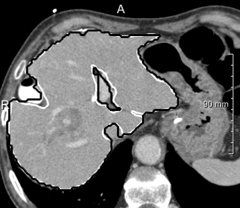
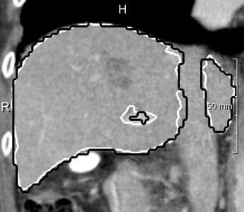
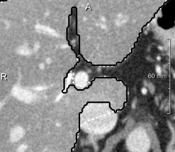
Figure 3: Example output of U-net ensemble trained on 2 mm voxel size (black) and reference (white); right: application on SLIVER07 case (dashed reference)

Example segmentations of the 2D U-net ensemble (2 mm) are illustrated in 3. Contour precision is limited by the resampling, but the model nicely excludes the vena cava and large hilar vessels much like in our training set. This hinders comparison against the state-of-art, since the reference masks from the SLIVER07 challenge (dashed in 3, right) partially include these vessels.

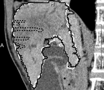
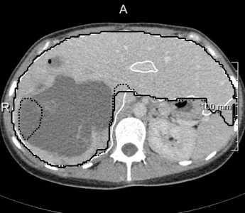
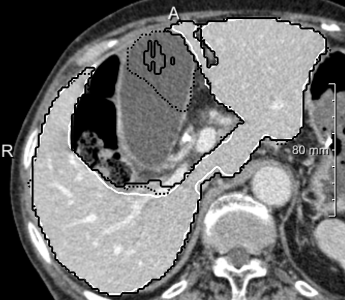
Figure 4: Example problems of slice-wise approach (dashed black) compared against ensemble of orthogonal U-nets (solid black) and reference (white)

In most cases, the purely slice-wise application of the 2D U-net (dashed contours in 4) does not show any comb artifacts in orthogonal views. However, the ensemble classifier (solid contours) performs significantly better when the appearance is severely abnormal and 3D context is needed. In some cases, it locally performs worse, but has an overall better volumetric overlap (Wilcoxon signed-rank test, $p<0.05$). The ensemble models performed significantly better than the purely 2D transversal model on the same voxel size.

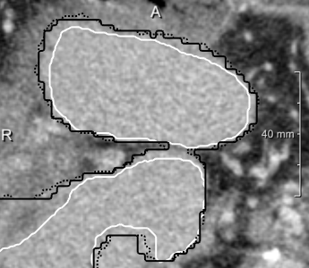
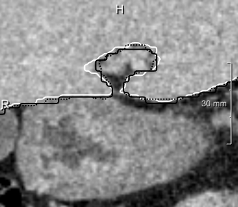
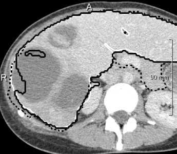
Figure 5: Left, center: Results from U-net ensembles on 2 mm (solid) and 1 mm voxel size (dashed); right: Comparison of 2D U-net (solid) and 3D U-net results (dashed)

We observed some problems with narrow fissures and gaps (5 left, center), and hypothesized that reducing the resampling target voxel size from 2 mm to 1 mm isotropic could help here. We could not observe qualitative changes, and the volumetric overlap did not change significantly. The MICCAI scores, however, showed significant improvements (Wilcoxon $p<0.05$) due to reduced surface distances, at the expense of higher GPU memory requirements and longer training and classification times.

mini-batch size		max tile size	(voxels)	padded size	(voxels)	ratio
2D U-net (4 levels)	21	$140\times 140$	411,600	$228\times 228$	1,091,664	38 %
2D U-net (5 levels)	16	$116\times 116$	215,296	$300\times 300$	1,440,000	15 %
3D U-net (4 levels)⋆	1	$20\times 20\times 20$	8,000	$108\times 108\times 108$	1,259,712	0.64 %
3D U-net (4 levels)	1	$68\times 60\times 20$	81,600	$156\times 148\times 108$	2,493,504	3.5 %
3D U-netpad (4 levels)	1	$104\times 104\times 64$	692,224	$104\times 104\times 64$	692,224	100 %

^⋆Naive variant, without reducing the number of filters in the downscaling path [12]

Table 2: Affordable batch sizes with 8 GiB of GPU memory

Lastly, we evaluated 3D U-nets, because slice-wise segmentation of volumetric images may lead to characteristic artifacts in general. However, both 3D U-nets performed significantly worse than the 2D ensembles. The 3D models performed better in some of the problematic areas of the 2D approaches (which were not many), but also brought new problems (5 right). We attribute this to the limits imposed by the available GPU memory on training batch sizes (2). U-nets with four resolution levels need 44 voxels of padding on each side, and when naively going from 2D to 3D (without reducing the number of filters [11, 12]), 8 GiB of memory are just enough to train with mini batches containing a single patch of 20³ voxels each, which does not suffice for stochastic gradient estimates stable enough for convergence. The ratio between the number of output voxels the loss is computed on and the number of input voxels after padding is given in the last column of 2. Consequently, the $\text{3D}_{\text{pad}}$ U-net performed significantly better than the 3D U-net with unpadded convolutions (Wilcoxon $p<0.05$).

With respect to the two loss functions that we investigated, we found that the Dice loss $L_{\text{DSC}}$ did not improve performance significantly in our experiments over binary cross entropy, even without any kind of class balancing. We offer the following explanation of this observation, considering a simple segmentation problem with perfect reference segmentations, but 95 % background class. Although a classifier always assigning the background class would achieve a low $L_{\text{CE}}$, all wrong voxels do contribute to $L_{\text{CE}}$, and the gradient $\vec{\nabla}L_{\text{CE}}$ points into the right direction. Only when given faulty or imprecise reference segmentations, or when the problem is ill-posed for some other reason, the classifier cannot perform well and will start to show a bias towards the more frequent class. We could observe this problem with other datasets, but not with the expert liver segmentations used here, which are of unusually high quality.

4 Conclusion

We have successfully implemented several CNN architectures for liver segmentation in CT, based on high-quality reference segmentation from surgery planning. We proposed an ensemble classifier comprising three 2D U-nets trained on orthogonal slices, which performed significantly better than a single 2D U-net, and was even more robust in the presence of abnormal cases such as resected or polycystic livers. Mean and median volumetric overlap was above 95 %, the MICCAI scores were higher than untrained humans, but apparently limited by the resampling we performed for efficiency, which impaired the surface distances.

Surprisingly, ensembles of orthogonal 2D U-nets performed even better than 3D U-nets trained on an NVIDIA GeForce GTX 1080 GPU, which we attribute to limits imposed by the available memory (8 GiB). Therefore, we conclude that a 2D classifier ensemble is an efficient approach for the time being, in particular when taking into account deployment scenarios in clinical environments without high-end hardware.

In the future, we want to improve the ensemble classifier by rescaling back to the original resolution and taking the original CT into account. Furthermore, we will investigate more efficient 3D CNNs [14] and extend the classifier towards vessels and tumors.

References

- [1] Schenk A, Haemmerich D, Preusser T. Planning of Image-Guided Interventions in the Liver. IEEE Pulse. 2011;2(5):48–55. doi:10.1109/MPUL.2011.942605.
- [2] Endo I, et al. Imaging and surgical planning for perihilar cholangiocarcinoma. Journal of Hepato-Biliary-Pancreatic Sciences. 2014;21(8):525–532. doi:10.1002/jhbp.75.
- [3] Heimann T, et al. Comparison and Evaluation of Methods for Liver Segmentation From CT Datasets. IEEE Transactions on Medical Imaging. 2009;28(8):1251–1265. doi:10.1109/tmi.2009.2013851.
- [4] Schenk A, et al. Efficient Semiautomatic Segmentation of 3D Objects in Medical Images. In: MICCAI 2000. vol. 1935 of LNCS. Springer; 2000. p. 186–195.
- [5] Kainmüller D, Lange T, Lamecker H. Shape constrained automatic segmentation of the liver based on a heuristic intensity model. In: Proc. MICCAI Workshop 3D Segmentation in the Clinic: A Grand Challenge; 2007. p. 109–116.
- [6] Heimann T, et al. A shape-guided deformable model with evolutionary algorithm initialization for 3D soft tissue segmentation. In: Biennial International Conference on Information Processing in Medical Imaging. Springer; 2007. p. 1–12.
- [7] Li G, Chen X, Shi F, Zhu W, Tian J, Xiang D. Automatic liver segmentation based on shape constraints and deformable graph cut in CT images. IEEE Transactions on Image Processing. 2015;24(12):5315–5329.
- [8] Christ P, et al. Automatic Liver and Lesion Segmentation in CT Using Cascaded Fully Convolutional Neural Networks and 3D Conditional Random Fields. In: MICCAI 2016. vol. 9901 of LNCS. Springer; 2016. p. 415–423.
- [9] Dou Q, Chen H, Jin Y, Yu L, Qin J, Heng PA. 3D Deeply Supervised Network for Automatic Liver Segmentation from CT Volumes. In: MICCAI 2016. vol. 9901 of LNCS. Springer; 2016. p. 149–157.
- [10] Long J, Shelhamer E, Darrell T. Fully Convolutional Networks for Semantic Segmentation. In: IEEE Conference on Computer Vision and Pattern Recognition (CVPR 2015). IEEE Computer Society; 2015. p. 3431–3440.
- [11] Ronneberger O, other. U-Net: Convolutional Networks for Biomedical Image Segmentation. In: MICCAI 2015. vol. 9351 of LNCS. Springer; 2015. p. 234–241.
- [12] Çiçek O, Abdulkadir A, Lienkamp S, Brox T, Ronneberger O. 3D U-Net: Learning Dense Volumetric Segmentation from Sparse Annotation. In: MICCAI 2016. vol. 9901 of LNCS. Springer; 2016. p. 424–432.
- [13] Milletari F, Navab N, Ahmadi SA. V-Net: Fully Convolutional Neural Networks for Volumetric Medical Image Segmentation. In: Intl. Conf. on 3D Vision (3DV 2016). IEEE Computer Society; 2016. p. 565–571.
- [14] Kamnitsas K, et al. Efficient multi-scale 3D CNN with fully connected CRF for accurate brain lesion segmentation. Medical Image Analysis. 2017;36:61–78. doi:10.1016/j.media.2016.10.004.
- [15] Prasoon A, Petersen K, Igel C, Lauze F, Dam E, Nielsen M. Deep feature learning for knee cartilage segmentation using a triplanar convolutional neural network. In: MICCAI 2013. vol. 16 of LNCS. Springer; 2013. p. 246–253.
- [16] Tanaka K, et al. Technique of right hemihepatectomy preserving ventral right anterior section guided by area of hepatic venous drainage. Surgery. 2010;147(3):450 – 458. doi:http://dx.doi.org/10.1016/j.surg.2009.04.020.
- [17] Luo W, Li Y, Urtasun R, Zemel R. Understanding the Effective Receptive Field in Deep Convolutional Neural Networks. In: NIPS 2016. Curran Associates Inc.; 2016. p. 4905–4913.
- [18] Kingma DP, Ba J. Adam: A Method for Stochastic Optimization. CoRR. 2014;abs/1412.6980.