On the Normal Force and Static Friction Acting on a Rolling Ball Actuated by Internal Point Masses

Abstract

The goal of this paper is to investigate the normal and tangential forces acting at the point of contact between a horizontal surface and a rolling ball actuated by internal point masses moving in the ball’s frame of reference. The normal force and static friction are derived from the equations of motion for a rolling ball actuated by internal point masses that move inside the ball’s frame of reference, and, as a special case, a rolling disk actuated by internal point masses. The masses may move along one-dimensional trajectories fixed in the ball’s and disk’s frame. The dynamics of a ball and disk actuated by masses moving along one-dimensional trajectories are simulated numerically and the minimum coefficients of static friction required to prevent slippage are computed.

Keywords: nonholonomic mechanics, holonomic mechanics, rolling balls, rolling disks
MSC2010 numbers: 37J60, 70E18, 70E60

1 Introduction

Internally actuated rolling ball robots hold great promise for environmental data collection, surveillance, and observation, such as is required for meteorology, law enforcement, security, defense, crop management, pollution detection, planetary exploration, etc. Many actuation mechanisms and control algorithms have been proposed for locomoting these robots, such as discussed in [1, 2] (internal rotors), [3] (internal magnets), [4] (internal gyroscopic pendulum), [5] (internal pendulum and yoke), [3, 6, 7, 8] (internal masses moving along linear trajectories), [9, 10] (internal masses moving along more general trajectories). When detachment from or slip at the surface occurs, the actuation mechanisms of rolling ball robots become inefficient. Moreover, from the perspective of theoretical mechanics, the consideration of the exact dynamics at the moment of slippage is quite difficult, as discussed in [11]. Some previous works have discussed these dynamics for non-actuated rolling ball robots. For example, progress has been made in the case of continuous slippage [12], but in general, it is always desirable to prevent dynamics that cause detachment or slippage. Thus, for example, the paper [13] investigates the magnitudes of the normal and tangential forces at the contact point for the non-actuated ball, in order to enforce the no-slip postulate and the main assumptions of nonholonomic mechanics. In this short paper, we will show how to calculate the normal force and static friction for a rolling ball actuated by moving internal point masses, so that the assumptions of no-detachment and no-slip at the contact point made in [10] may be readily checked. The expressions for the normal and tangential forces at the contact point obtained here, we hope, will facilitate practical implementations of rolling ball robots that obey the performance envelope defined by the no-detachment and no-slip conditions.

There are 3 regimes for the dynamics of a ball actuated by moving internal point masses:

1. Rolling without Slipping These dynamics and their associated contact point forces are the main focus of this paper and are derived in Section 2.

2. Detachment These dynamics are derived in Appendix B.

3. Sliding Friction and the Painlevé Paradox This paradox corresponds to the impossibility to uniquely continue the solution past certain boundaries in phase space if dry friction at the contact point is assumed.

The second item deals with the detachment dynamics when the ball loses contact with and leaves the surface. In that case, the forces applied on the ball at the moment of detachment are discontinuous and the numerical solution of the problem is challenging. The third item above, the description of a system experiencing dry sliding friction at the contact point, leads to the Painlevé paradox. Even for simple dynamical systems such as a falling rigid rod whose end slides on the plane with friction, there is the impossibility of continuing the dynamics using both the condition of contact and the laws of sliding friction, provided that the coefficient of static friction $\mu_{\mathrm{s}}$ is large enough. For the implementation of the nonholonomic constraint, that coefficient is taken to be very large (or even infinite). For discussion and resolution of these highly complex issues of contact dynamics, see [14, 15, 16, 17]. Our mechanical system is substantially more complex than the one considered by Painlevé, and thus careful treatment of the dynamics’ continuation through detachment is beyond the scope of this paper.

In order for a ball to roll without slipping on a horizontal surface so that the rolling constraint is in effect, the magnitude $N$ of the normal force of the surface acting at the ball’s contact point must be positive (i.e. the normal force direction must oppose gravity’s direction) so that

$$N>0.$$ (1.1)

In addition, to prevent slipping, an inequality constraint due to dry static friction must be satisfied:

$$\mu_{\mathrm{s}}N\geq f_{\mathrm{s}},$$ (1.2)

where $\mu_{\mathrm{s}}$ is the coefficient of static friction and $f_{\mathrm{s}}$ is the magnitude of the static friction. $\mu_{\mathrm{s}}$ is positive and depends on the material properties of the ball and surface and possibly on other environmental factors. The condition (1.2) for dry static friction acting at the contact point is a simplified model, following from Amontons’ laws [18]. While finer aspects of the behavior of dry static friction acting at the contact point are certainly known, we shall use condition (1.2) to enforce the no-slip dynamics, as it is the most widely used and accepted. In reality, the true relationship between the normal and tangential forces is substantially more complicated than (1.2) and is still up for considerable debate. The transition from no-slip to slipping motion is rather complex, and we do not attempt to study it here. We refer the reader to recent papers by V.V. Kozlov [19, 20], which explain the complexity of the mechanism of sliding friction and treat associated paradoxes arising from naive applications of dry friction laws.

Therefore, any numerical simulation of the dynamics of a rolling ball, especially one actuated by an internal mechanism such as moving internal point masses, must verify that $N>0$ to ensure that the rolling constraint is indeed always in effect. Moreover, if $N>0$ for $a\leq t\leq b$ and if $\mu_{\mathrm{s}}$ is unknown, it is also useful to compute

$$\hat{\mu}_{\mathrm{s}}\equiv\max_{a\leq t\leq b}\frac{f_{\mathrm{s}}}{N},$$ (1.3)

which is the minimum coefficient of static friction permitted before slippage occurs. If $\mu_{\mathrm{s}}$ is known and if the ball has an internal actuation mechanism that may be controlled, in order to construct a control for the ball such that the ball rolls without slipping, it is necessary to include the constraints $N>0$ and $\mu_{\mathrm{s}}N\geq f_{\mathrm{s}}$ in conjunction with the no-slip dynamics. In order to enable these computations, this paper derives the normal force and static friction acting on a ball actuated by internal point masses, whose dynamics were investigated in [10], assuming that this ball rolls without slipping. In the process, the ball’s equations of motion are derived via Newton’s laws, validating a previous derivation via Lagrange-d’Alembert’s principle in [10]. We shall note that reference [21] derived the normal force acting on a ball actuated by a single spherical pendulum. The present work generalizes the computation of the normal force to the case when the ball is actuated by masses moving along arbitrary trajectories.

2 Rolling Ball with 3-d Parameterizations of the Point Mass Trajectories

This section pedagogically derives the equations of motion of a rolling ball, defining the coordinate systems, notation, and variables, generalizing the derivations in [9], and validating the derivation in [10] obtained via Lagrange-d’Alembert’s principle.

Consider a rigid ball of radius $r$ containing some static internal structure as well as $n\in\mathbb{N}^{0}$ point masses which are free to move inside the ball, where $\mathbb{N}^{0}$ denotes the set of nonnegative integers. This ball rolls without slipping on a horizontal surface in the presence of a uniform gravitational field. The ball with its static internal structure has mass $m_{0}$ and the $i^{\mathrm{th}}$ point mass has mass $m_{i}$ for $1\leq i\leq n$. Let $M=\sum_{i=0}^{n}m_{i}$ denote the mass of the total system. The total mechanical system consisting of the ball with its static internal structure and the $n$ point masses is referred to as the ball or the rolling ball, the ball with its static internal structure but without the $n$ point masses may also be referred to as $m_{0}$, and the $i^{\mathrm{th}}$ point mass may also be referred to as $m_{i}$ for $1\leq i\leq n$. Note that the dynamics of this system are equivalent to that of the Chaplygin ball [22, 10], equipped with point masses.

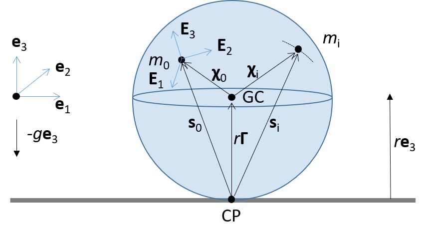
Figure 2.2: A ball of radius $r$ and mass $m_{0}$ rolls without slipping on a horizontal surface in the presence of a uniform gravitational field of magnitude $g$. The ball’s geometric center, center of mass, and contact point with the horizontal surface are denoted by GC, $m_{0}$, and CP, respectively. The ball’s motion is actuated by $n$ point masses, each of mass $m_{i}$, $1\leq i\leq n$, that move inside the ball. The spatial frame has origin located at height $r$ above the horizontal surface and orthonormal axes $\mathbf{e}_{1}$, $\mathbf{e}_{2}$, and $\mathbf{e}_{3}$. The body frame has origin located at the ball’s center of mass (denoted by $m_{0}$) and orthonormal axes $\mathbf{E}_{1}$, $\mathbf{E}_{2}$, and $\mathbf{E}_{3}$. All vectors inside the ball are expressed with respect to the body frame, while all vectors outside the ball are expressed with respect to the spatial frame.

Two coordinate systems, or frames of reference, will be used to describe the motion of the rolling ball, an inertial spatial coordinate system and a body coordinate system in which each particle within the ball is always fixed. For brevity, the spatial coordinate system will be referred to as the spatial frame and the body coordinate system will be referred to as the body frame. These two frames are depicted in Figure 2.2. The spatial frame has orthonormal axes $\mathbf{e}_{1}$, $\mathbf{e}_{2}$, $\mathbf{e}_{3}$, such that the $\mathbf{e}_{1}$-$\mathbf{e}_{2}$ plane is parallel to the horizontal surface and passes through the ball’s geometric center (i.e. the $\mathbf{e}_{1}$-$\mathbf{e}_{2}$ plane is a height $r$ above the horizontal surface), such that $\mathbf{e}_{3}$ is vertical (i.e. $\mathbf{e}_{3}$ is perpendicular to the horizontal surface) and points “upward” and away from the horizontal surface, and such that $\left(\mathbf{e}_{1},\mathbf{e}_{2},\mathbf{e}_{3}\right)$ forms a right-handed coordinate system. For simplicity, the spatial frame axes are chosen to be

$$\mathbf{e}_{1}=\begin{bmatrix}1&0&0\end{bmatrix}^{\mathsf{T}},\quad\mathbf{e}_{2}=\begin{bmatrix}0&1&0\end{bmatrix}^{\mathsf{T}},\quad\mathrm{and}\quad\mathbf{e}_{3}=\begin{bmatrix}0&0&1\end{bmatrix}^{\mathsf{T}}.$$ (2.1)

The acceleration due to gravity in the uniform gravitational field is $\mathfrak{g}=-g\mathbf{e}_{3}=\begin{bmatrix}0&0&-g\end{bmatrix}^{\mathsf{T}}$ in the spatial frame.

The body frame’s origin is chosen to coincide with the position of $m_{0}$’s center of mass. The body frame has orthonormal axes $\mathbf{E}_{1}$, $\mathbf{E}_{2}$, and $\mathbf{E}_{3}$, chosen to coincide with $m_{0}$’s principal axes, in which $m_{0}$’s inertia tensor $\mathbb{I}$ is diagonal, with corresponding principal moments of inertia $d_{1}$, $d_{2}$, and $d_{3}$. That is, in this body frame the inertia tensor is the diagonal matrix $\mathbb{I}=\mathrm{\textbf{diag}}\left(\begin{bmatrix}d_{1}&d_{2}&d_{3}\end{bmatrix}\right)$. Moreover, $\mathbf{E}_{1}$, $\mathbf{E}_{2}$, and $\mathbf{E}_{3}$ are chosen so that $\left(\mathbf{E}_{1},\mathbf{E}_{2},\mathbf{E}_{3}\right)$ forms a right-handed coordinate system. For simplicity, the body frame axes are chosen to be

$$\mathbf{E}_{1}=\begin{bmatrix}1&0&0\end{bmatrix}^{\mathsf{T}},\quad\mathbf{E}_{2}=\begin{bmatrix}0&1&0\end{bmatrix}^{\mathsf{T}},\quad\mathrm{and}\quad\mathbf{E}_{3}=\begin{bmatrix}0&0&1\end{bmatrix}^{\mathsf{T}}.$$ (2.2)

In the spatial frame, the body frame is the moving frame $\left(\Lambda\left(t\right)\mathbf{E}_{1},\Lambda\left(t\right)\mathbf{E}_{2},\Lambda\left(t\right)\mathbf{E}_{3}\right)$, where $\Lambda\left(t\right)\in SO(3)$ defines the orientation (or attitude) of the ball at time $t$ relative to its reference configuration, for example at some initial time.

For $0\leq i\leq n$, let $\mathbf{z}_{i}(t)$ denote the position of $m_{i}$’s center of mass in the spatial frame. Let $\boldsymbol{\chi}_{i}(t)$ denote the body frame vector from the ball’s geometric center to $m_{i}$’s center of mass. Then for $m_{0}$, $\boldsymbol{\chi}_{0}$ is the constant (time-independent) vector from the ball’s geometric center to $m_{0}$’s center of mass. Note that the position of $m_{i}$’s center of mass in the body frame is $\boldsymbol{\chi}_{i}(t)-\boldsymbol{\chi}_{0}$ and in the spatial frame is $\mathbf{z}_{i}(t)=\mathbf{z}_{0}(t)+\Lambda(t)\left[\boldsymbol{\chi}_{i}(t)-\boldsymbol{\chi}_{0}\right]$. In general, a particle with position $\mathbf{w}(t)$ in the body frame has position $\mathbf{z}(t)=\mathbf{z}_{0}(t)+\Lambda(t)\mathbf{w}(t)$ in the spatial frame and has position $\mathbf{w}(t)+\boldsymbol{\chi}_{0}$ in the body frame translated to the ball’s geometric center. In addition, suppose a time-varying external force $\mathbf{F}_{\mathrm{e}}(t)$ acts at the ball’s geometric center. Note that $\mathbf{F}_{\mathrm{e}}(t)$ does not involve the static friction induced by the surface to enforce the no-slip constraint. Instead, it involves forces due to other environmental factors such as air resistance (i.e. drag) and wind force.

To obtain the dynamics of this rolling ball, it is assumed that the trajectories $\left\{\boldsymbol{\chi}_{i}(t)\right\}_{i=1}^{n}$ of the $n$ point masses are prescribed, in which case the dynamics can be obtained more efficiently by considering a single point mass of mass $M-m_{0}$ and whose trajectory is $\frac{1}{M-m_{0}}\sum_{i=1}^{n}m_{i}\boldsymbol{\chi}_{i}(t)$, the center of mass of the trajectories of the $n$ point masses. In subsequent work [23], we consider the control of this rolling ball, in which case it is desirable to have $n$ degrees of freedom instead of a single degree of freedom. In the current work, the ball’s motion is not controlled.

It is also worth noting the validity of the assumption that $\boldsymbol{\chi}_{i}(t)$ is a prescribed function of time for $1\leq i\leq n$. In general, for internal masses actuated by motors with a given torque, the motion of the masses as a function of time cannot be prescribed a priori, but instead must be solved for in conjunction with the ball’s motion [24]. We envision a different driving mechanism based on a stepper motor which is rigidly attached to the internal frame of the rolling ball. Unlike a regular electric motor which generates a given torque based on the input voltage/current, a stepper motor is a device which rotates the motor’s shaft by a given amount measured in a discrete number of steps, where each step is typically 1-2 degrees depending on the motor’s design, with a typical error of 1-2% of the step angle. The maximum achievable rotation speed is dependent on the motor’s type and the masses involved. Modern stepper motors are capable of turning quite rapidly, at least several full revolutions per second and possibly more depending on the torques applied to the shaft. Thus, as long as the motor used is capable of supplying the torques required, we can assume that the rotation of the motor’s shaft with respect to the ball can be specified within a given accuracy as a function of time, independent of the motion of the ball itself. This rotation of the shaft can then be used to drive masses along different trajectories fixed in the ball’s frame. Some examples of driving mechanisms of this type are illustrated in Figure 2.1. In the left panel of Figure 2.1, the stepper motor swings a pendulum, so that the trajectory of the mass is a circle. In the right panel of Figure 2.1, the stepper motor translates a rod with masses attached along a line. It is possible to create more complex trajectories, for example, by using a curved toothed rod instead of the straight one depicted in the right panel of Figure 2.1.

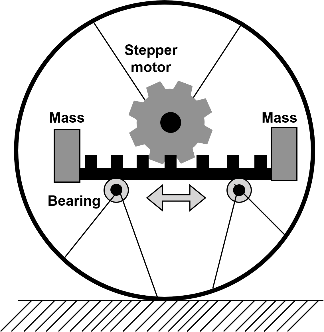
Figure 2.1: Examples of driving mechanisms actuated by a stepper motor. In both cases, the motor is rigidly attached to the internal frame of the ball, with the angle of rotation of the motor’s shaft prescribed as a function of time. Left: a stepper motor swings a pendulum. Right: A stepper motor uses a sprocket to translate a rigid toothed rod with masses attached.

Let us turn to the dynamical description of the ball’s motion. For conciseness, the ball’s geometric center is often denoted GC, $m_{0}$’s center of mass is often denoted CM, and the ball’s contact point with the surface is often denoted CP. The GC is located at $\mathbf{z}_{\mathrm{GC}}(t)=\mathbf{z}_{0}(t)-\Lambda(t)\boldsymbol{\chi}_{0}$ in the spatial frame, at $-\boldsymbol{\chi}_{0}$ in the body frame, and at $\mathbf{0}$ in the body frame translated to the GC. The CM is located at $\mathbf{z}_{0}(t)$ in the spatial frame, at $\mathbf{0}$ in the body frame, and at $\boldsymbol{\chi}_{0}$ in the body frame translated to the GC. The CP is located at $\mathbf{z}_{\mathrm{CP}}(t)=\mathbf{z}_{0}(t)-\Lambda(t)\left[r\boldsymbol{\Gamma}(t)+\boldsymbol{\chi}_{0}\right]$ in the spatial frame, at $-\left[r\boldsymbol{\Gamma}(t)+\boldsymbol{\chi}_{0}\right]$ in the body frame, and at $-r\boldsymbol{\Gamma}(t)$ in the body frame translated to the GC, where $\boldsymbol{\Gamma}(t)\equiv\Lambda^{-1}(t)\mathbf{e}_{3}$. Since the third spatial coordinate of the ball’s GC is always $0$ and of the ball’s CP is always $-r$, only the first two spatial coordinates of the ball’s GC and CP, denoted by $\boldsymbol{z}(t)$, are needed to determine the spatial location of the ball’s GC and CP.

For succintness, the explicit time dependence of variables is often dropped. That is, the orientation of the ball at time $t$ is denoted simply $\Lambda$ rather than $\Lambda(t)$, the position of $m_{i}$’s center of mass in the spatial frame at time $t$ is denoted $\mathbf{z}_{i}$ rather than $\mathbf{z}_{i}(t)$, the position of $m_{i}$’s center of mass in the body frame translated to the GC at time $t$ is denoted $\boldsymbol{\chi}_{i}$ rather than $\boldsymbol{\chi}_{i}(t)$, the spatial $\mathbf{e}_{1}$- and $\mathbf{e}_{2}$-components of the ball’s GC and CP at time $t$ are denoted $\boldsymbol{z}$ rather than $\boldsymbol{z}(t)$, and the external force is denoted $\mathbf{F}_{\mathrm{e}}$ rather than $\mathbf{F}_{\mathrm{e}}(t)$.

Recall that $N$ denotes the magnitude of the normal force acting at the ball’s CP. Assume that the ball rolls without slipping so that $N>0$ and

$${\dot{\mathbf{z}}}_{\mathrm{GC}}=\Lambda\boldsymbol{\Omega}\times r\mathbf{e}_{3}=\Lambda\left[\boldsymbol{\Omega}\times r\boldsymbol{\Gamma}\right],$$ (2.3)

where $\boldsymbol{\Omega}\equiv\left(\Lambda^{-1}\dot{\Lambda}\right)^{\vee}$ is the ball’s body angular velocity and $\boldsymbol{\Gamma}\equiv\Lambda^{-1}\mathbf{e}_{3}$. Recall that $f_{\mathrm{s}}$ denotes the magnitude of the static friction acting at the ball’s CP and let $\boldsymbol{\sigma}$ denote the unit-length direction antiparallel to the static friction. Note that $\boldsymbol{\sigma}$ is parallel to the surface and therefore orthogonal to $\mathbf{e}_{3}$. Newton’s laws for linear motion state that the time derivative of the ball’s spatial linear momentum equals the sum of the forces exerted on the ball. Figure 2.3 illustrates the free body diagram depicting all the forces acting on the ball. Since the ball of mass $m_{0}$ is acted upon by gravity at the ball’s CM, by an external force $\mathbf{F}_{\mathrm{e}}$ at the ball’s GC, by a normal force $N\mathbf{e}_{3}$ at the ball’s CP, and by a static friction $-f_{\mathrm{s}}\boldsymbol{\sigma}$ at the ball’s CP and since each point mass $m_{i}$, for $1\leq i\leq n$, is acted upon by gravity and has spatial acceleration ${\ddot{\mathbf{z}}}_{i}$, Newton’s laws for linear motion give the time derivative of the ball’s spatial linear momentum as

$$\frac{\mathrm{d}}{\mathrm{d}t}\left(m_{0}{\dot{\mathbf{z}}}_{0}\right)=\left(N-Mg\right)\mathbf{e}_{3}+\mathbf{F}_{\mathrm{e}}-f_{\mathrm{s}}\boldsymbol{\sigma}-\sum_{i=1}^{n}m_{i}{\ddot{\mathbf{z}}}_{i}.$$ (2.4)

Since $m_{0}$ is constant, $\frac{\mathrm{d}}{\mathrm{d}t}\left(m_{0}{\dot{\mathbf{z}}}_{0}\right)=m_{0}{\ddot{\mathbf{z}}}_{0}$ and (2.4) simplifies to

$$\mathbf{0}=\left(N-Mg\right)\mathbf{e}_{3}+\mathbf{F}_{\mathrm{e}}-f_{\mathrm{s}}\boldsymbol{\sigma}-\sum_{i=0}^{n}m_{i}{\ddot{\mathbf{z}}}_{i}.$$ (2.5)

For $0\leq i\leq n$, recall that

$$\mathbf{z}_{i}=\mathbf{z}_{\mathrm{GC}}+\Lambda\boldsymbol{\chi}_{i}.$$ (2.6)

Differentiating (2.6) with respect to time, using the rolling constraint (2.3), and recalling that $\dot{\Lambda}=\Lambda\widehat{\boldsymbol{\Omega}}$ (since $\boldsymbol{\Omega}\equiv\left(\Lambda^{-1}\dot{\Lambda}\right)^{\vee}$) and $\mathbf{s}_{i}\equiv r\boldsymbol{\Gamma}+\boldsymbol{\chi}_{i}$ yield

$${\dot{\mathbf{z}}}_{i}={\dot{\mathbf{z}}}_{\mathrm{GC}}+\dot{\Lambda}\boldsymbol{\chi}_{i}+\Lambda{\dot{\boldsymbol{\chi}}}_{i}=\Lambda\left[\boldsymbol{\Omega}\times r\boldsymbol{\Gamma}\right]+\Lambda\widehat{\boldsymbol{\Omega}}\boldsymbol{\chi}_{i}+\Lambda{\dot{\boldsymbol{\chi}}}_{i}=\Lambda\left[\boldsymbol{\Omega}\times\mathbf{s}_{i}+{\dot{\boldsymbol{\chi}}}_{i}\right].$$ (2.7)

Differentiating (2.7) with respect to time, using $\dot{\Lambda}=\Lambda\widehat{\boldsymbol{\Omega}}$, $\mathbf{s}_{i}\equiv r\boldsymbol{\Gamma}+\boldsymbol{\chi}_{i}$, and ${\dot{\mathbf{s}}}_{i}=r\dot{\boldsymbol{\Gamma}}+{\dot{\boldsymbol{\chi}}}_{i}$, and recalling that $\dot{\boldsymbol{\Gamma}}=\boldsymbol{\Gamma}\times\boldsymbol{\Omega}$ (since $\dot{\boldsymbol{\Gamma}}=\left(\frac{\mathrm{d}}{\mathrm{d}t}\Lambda^{-1}\right)\mathbf{e}_{3}=-\Lambda^{-1}\dot{\Lambda}\Lambda^{-1}\mathbf{e}_{3}=-\widehat{\boldsymbol{\Omega}}\boldsymbol{\Gamma}=-\boldsymbol{\Omega}\times\boldsymbol{\Gamma}=\boldsymbol{\Gamma}\times\boldsymbol{\Omega}$) yield

$$\begin{split}{\ddot{\mathbf{z}}}_{i}&=\Lambda\left[\dot{\boldsymbol{\Omega}}\times\mathbf{s}_{i}+\boldsymbol{\Omega}\times{\dot{\mathbf{s}}}_{i}+{\ddot{\boldsymbol{\chi}}}_{i}\right]+\dot{\Lambda}\left[\boldsymbol{\Omega}\times\mathbf{s}_{i}+{\dot{\boldsymbol{\chi}}}_{i}\right]\\ &=\Lambda\left[\dot{\boldsymbol{\Omega}}\times\mathbf{s}_{i}+\boldsymbol{\Omega}\times{\dot{\mathbf{s}}}_{i}+{\ddot{\boldsymbol{\chi}}}_{i}\right]+\Lambda\widehat{\boldsymbol{\Omega}}\left[\boldsymbol{\Omega}\times\mathbf{s}_{i}+{\dot{\boldsymbol{\chi}}}_{i}\right]\\ &=\Lambda\left[\dot{\boldsymbol{\Omega}}\times\mathbf{s}_{i}+\boldsymbol{\Omega}\times\left(\boldsymbol{\Omega}\times\mathbf{s}_{i}+{\dot{\boldsymbol{\chi}}}_{i}+{\dot{\mathbf{s}}}_{i}\right)+{\ddot{\boldsymbol{\chi}}}_{i}\right]\\ &=\Lambda\left[\dot{\boldsymbol{\Omega}}\times\mathbf{s}_{i}+\boldsymbol{\Omega}\times\left(\boldsymbol{\Omega}\times\left(r\boldsymbol{\Gamma}+\boldsymbol{\chi}_{i}\right)+{\dot{\boldsymbol{\chi}}}_{i}+r\dot{\boldsymbol{\Gamma}}+{\dot{\boldsymbol{\chi}}}_{i}\right)+{\ddot{\boldsymbol{\chi}}}_{i}\right]\\ &=\Lambda\left[\dot{\boldsymbol{\Omega}}\times\mathbf{s}_{i}+\boldsymbol{\Omega}\times\left(\boldsymbol{\Omega}\times\boldsymbol{\chi}_{i}+2{\dot{\boldsymbol{\chi}}}_{i}\right)+{\ddot{\boldsymbol{\chi}}}_{i}\right].\end{split}$$ (2.8)

Substituting (2.8) into (2.5) gives

$$\mathbf{0}=\left(N-Mg\right)\mathbf{e}_{3}+\mathbf{F}_{\mathrm{e}}-f_{\mathrm{s}}\boldsymbol{\sigma}-\Lambda\sum_{i=0}^{n}m_{i}\left[\dot{\boldsymbol{\Omega}}\times\mathbf{s}_{i}+\boldsymbol{\Omega}\times\left(\boldsymbol{\Omega}\times\boldsymbol{\chi}_{i}+2{\dot{\boldsymbol{\chi}}}_{i}\right)+{\ddot{\boldsymbol{\chi}}}_{i}\right].$$ (2.9)

Dotting both sides of (2.9) with $\mathbf{e}_{3}$, recalling that $\boldsymbol{\sigma}$ is orthogonal to $\mathbf{e}_{3}$, and solving for $N$ gives

$$N=Mg+\left<\sum_{i=0}^{n}m_{i}\left[\dot{\boldsymbol{\Omega}}\times\mathbf{s}_{i}+\boldsymbol{\Omega}\times\left(\boldsymbol{\Omega}\times\boldsymbol{\chi}_{i}+2{\dot{\boldsymbol{\chi}}}_{i}\right)+{\ddot{\boldsymbol{\chi}}}_{i}\right],\boldsymbol{\Gamma}\right>-F_{\mathrm{e},3}.$$ (2.10)

Solving (2.9) for $-f_{\mathrm{s}}\boldsymbol{\sigma}$ and substituting the formula for $N$ given by (2.10) yield

$$-f_{\mathrm{s}}\boldsymbol{\sigma}=\begin{bmatrix}\left(\Lambda\sum_{i=0}^{n}m_{i}\left[\dot{\boldsymbol{\Omega}}\times\mathbf{s}_{i}+\boldsymbol{\Omega}\times\left(\boldsymbol{\Omega}\times\boldsymbol{\chi}_{i}+2{\dot{\boldsymbol{\chi}}}_{i}\right)+{\ddot{\boldsymbol{\chi}}}_{i}\right]-\mathbf{F}_{\mathrm{e}}\right)_{12}\\ 0\end{bmatrix}.$$ (2.11)

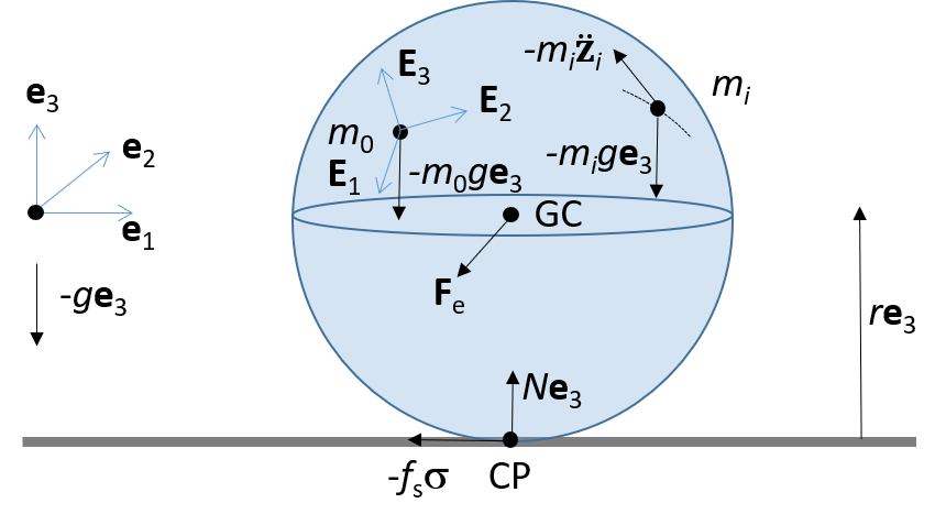
Figure 2.3: Free body diagram showing all the forces that act on the ball depicted in Figure 2.2.

Newton’s laws for angular motion state that the time derivative of the ball’s spatial angular momentum, computed about the ball’s CM, equals the sum of the torques exerted on the ball about the ball’s CM. Equating the time derivative of the ball’s spatial angular momentum, computed about the ball’s CM, to the sum of the torques about the ball’s CM yields

$$\frac{\mathrm{d}}{\mathrm{d}t}\left(\mathbb{I}_{\mathrm{S}}\boldsymbol{\omega}\right)=-\Lambda\mathbf{s}_{0}\times\left(N\mathbf{e}_{3}-f_{\mathrm{s}}\boldsymbol{\sigma}\right)-\Lambda\boldsymbol{\chi}_{0}\times\mathbf{F}_{\mathrm{e}}+\sum_{i=1}^{n}\left(\mathbf{z}_{i}-\mathbf{z}_{0}\right)\times m_{i}\left(-{\ddot{\mathbf{z}}}_{i}-g\mathbf{e}_{3}\right),$$ (2.12)

where $\mathbb{I}_{\mathrm{S}}$ is the ball’s spatial moment of inertia and $\boldsymbol{\omega}\equiv\left[\dot{\Lambda}\Lambda^{-1}\right]^{\vee}$ is the ball’s spatial angular velocity. By definition, the ball’s body moment of inertia is $\mathbb{I}\equiv\Lambda^{-1}\mathbb{I}_{\mathrm{S}}\Lambda$, so that $\mathbb{I}_{\mathrm{S}}=\Lambda\mathbb{I}\Lambda^{-1}$. By definition, $\boldsymbol{\omega}\equiv\left[\dot{\Lambda}\Lambda^{-1}\right]^{\vee}=\Lambda\boldsymbol{\Omega}$, so that $\dot{\boldsymbol{\omega}}=\dot{\Lambda}\boldsymbol{\Omega}+\Lambda\dot{\boldsymbol{\Omega}}=\Lambda\widehat{\boldsymbol{\Omega}}\boldsymbol{\Omega}+\Lambda\dot{\boldsymbol{\Omega}}=\Lambda\left(\boldsymbol{\Omega}\times\boldsymbol{\Omega}\right)+\Lambda\dot{\boldsymbol{\Omega}}=\Lambda\dot{\boldsymbol{\Omega}}$, recalling that $\dot{\Lambda}=\Lambda\widehat{\boldsymbol{\Omega}}$. Also recall that $\dot{\Lambda}^{-1}=-\Lambda^{-1}\dot{\Lambda}\Lambda^{-1}$. Using these facts, the time derivative of the ball’s spatial angular momentum, computed about the ball’s CM, may be simplified:

$$\begin{split}\frac{\mathrm{d}}{\mathrm{d}t}\left(\mathbb{I}_{\mathrm{S}}\boldsymbol{\omega}\right)&=\dot{\mathbb{I}}_{\mathrm{S}}\boldsymbol{\omega}+\mathbb{I}_{\mathrm{S}}\dot{\boldsymbol{\omega}}=\left(\dot{\Lambda}\mathbb{I}\Lambda^{-1}+\Lambda\mathbb{I}\dot{\Lambda}^{-1}\right)\Lambda\boldsymbol{\Omega}+\Lambda\mathbb{I}\Lambda^{-1}\Lambda\dot{\boldsymbol{\Omega}}\\ &=\left(\dot{\Lambda}\mathbb{I}\Lambda^{-1}-\Lambda\mathbb{I}\Lambda^{-1}\dot{\Lambda}\Lambda^{-1}\right)\Lambda\boldsymbol{\Omega}+\Lambda\mathbb{I}\dot{\boldsymbol{\Omega}}\\ &=\left(\Lambda\widehat{\boldsymbol{\Omega}}\mathbb{I}-\Lambda\mathbb{I}\Lambda^{-1}\Lambda\widehat{\boldsymbol{\Omega}}\right)\boldsymbol{\Omega}+\Lambda\mathbb{I}\dot{\boldsymbol{\Omega}}=\Lambda\left(\boldsymbol{\Omega}\times\mathbb{I}\boldsymbol{\Omega}+\mathbb{I}\dot{\boldsymbol{\Omega}}\right).\end{split}$$ (2.13)

Substituting (2.13) into (2.12) yields

$$\Lambda\left(\boldsymbol{\Omega}\times\mathbb{I}\boldsymbol{\Omega}+\mathbb{I}\dot{\boldsymbol{\Omega}}\right)=-\Lambda\mathbf{s}_{0}\times\left(N\mathbf{e}_{3}-f_{\mathrm{s}}\boldsymbol{\sigma}\right)-\Lambda\boldsymbol{\chi}_{0}\times\mathbf{F}_{\mathrm{e}}-\sum_{i=1}^{n}\left(\mathbf{z}_{i}-\mathbf{z}_{0}\right)\times m_{i}\left({\ddot{\mathbf{z}}}_{i}+g\mathbf{e}_{3}\right).$$ (2.14)

Multiplying (2.14) by $\Lambda^{-1}$, using (2.6), and recalling that $\mathbf{s}_{0}\equiv r\boldsymbol{\Gamma}+\boldsymbol{\chi}_{0}$ and $\tilde{\boldsymbol{\Gamma}}\equiv\Lambda^{-1}\mathbf{F}_{\mathrm{e}}$ yield

$$\boldsymbol{\Omega}\times\mathbb{I}\boldsymbol{\Omega}+\mathbb{I}\dot{\boldsymbol{\Omega}}=-\left(r\boldsymbol{\Gamma}+\boldsymbol{\chi}_{0}\right)\times\Lambda^{-1}\left(N\mathbf{e}_{3}-f_{\mathrm{s}}\boldsymbol{\sigma}\right)-\boldsymbol{\chi}_{0}\times\tilde{\boldsymbol{\Gamma}}-\sum_{i=1}^{n}\left(\boldsymbol{\chi}_{i}-\boldsymbol{\chi}_{0}\right)\times m_{i}\left(\Lambda^{-1}{\ddot{\mathbf{z}}}_{i}+g\boldsymbol{\Gamma}\right).$$ (2.15)

Solving (2.5) for $N\mathbf{e}_{3}-f_{\mathrm{s}}\boldsymbol{\sigma}$, which is the net force exerted by the surface on the ball at the CP, yields

$$N\mathbf{e}_{3}-f_{\mathrm{s}}\boldsymbol{\sigma}=Mg\mathbf{e}_{3}-\mathbf{F}_{\mathrm{e}}+\sum_{i=0}^{n}m_{i}{\ddot{\mathbf{z}}}_{i}=\sum_{i=0}^{n}m_{i}\left({\ddot{\mathbf{z}}}_{i}+g\mathbf{e}_{3}\right)-\mathbf{F}_{\mathrm{e}}.$$ (2.16)

Multiplying (2.16) by $\Lambda^{-1}$ yields

$$\Lambda^{-1}\left(N\mathbf{e}_{3}-f_{\mathrm{s}}\boldsymbol{\sigma}\right)=\sum_{i=0}^{n}m_{i}\left(\Lambda^{-1}{\ddot{\mathbf{z}}}_{i}+g\boldsymbol{\Gamma}\right)-\tilde{\boldsymbol{\Gamma}}.$$ (2.17)

Substituting (2.17) into (2.15) yields

$$\begin{split}\boldsymbol{\Omega}\times\mathbb{I}\boldsymbol{\Omega}+\mathbb{I}\dot{\boldsymbol{\Omega}}&=-\left(r\boldsymbol{\Gamma}+\boldsymbol{\chi}_{0}\right)\times\left[\sum_{i=0}^{n}m_{i}\left(\Lambda^{-1}{\ddot{\mathbf{z}}}_{i}+g\boldsymbol{\Gamma}\right)-\tilde{\boldsymbol{\Gamma}}\right]-\boldsymbol{\chi}_{0}\times\tilde{\boldsymbol{\Gamma}}\\ &\hphantom{=}-\sum_{i=1}^{n}\left(\boldsymbol{\chi}_{i}-\boldsymbol{\chi}_{0}\right)\times m_{i}\left(\Lambda^{-1}{\ddot{\mathbf{z}}}_{i}+g\boldsymbol{\Gamma}\right)\\ &=-r\boldsymbol{\Gamma}\times\left[\sum_{i=0}^{n}m_{i}\left(\Lambda^{-1}{\ddot{\mathbf{z}}}_{i}+g\boldsymbol{\Gamma}\right)-\tilde{\boldsymbol{\Gamma}}\right]-\sum_{i=0}^{n}\boldsymbol{\chi}_{i}\times m_{i}\left(\Lambda^{-1}{\ddot{\mathbf{z}}}_{i}+g\boldsymbol{\Gamma}\right)\\ &=-\sum_{i=0}^{n}m_{i}\mathbf{s}_{i}\times\left(\Lambda^{-1}{\ddot{\mathbf{z}}}_{i}+g\boldsymbol{\Gamma}\right)+r\boldsymbol{\Gamma}\times\tilde{\boldsymbol{\Gamma}}.\end{split}$$ (2.18)

Substituting (2.8) into (2.18) yields

$$\begin{split}\boldsymbol{\Omega}\times\mathbb{I}\boldsymbol{\Omega}+\mathbb{I}\dot{\boldsymbol{\Omega}}&=-\sum_{i=0}^{n}m_{i}\mathbf{s}_{i}\times\left\{\dot{\boldsymbol{\Omega}}\times\mathbf{s}_{i}+\boldsymbol{\Omega}\times\left(\boldsymbol{\Omega}\times\boldsymbol{\chi}_{i}+2{\dot{\boldsymbol{\chi}}}_{i}\right)+{\ddot{\boldsymbol{\chi}}}_{i}+g\boldsymbol{\Gamma}\right\}+r\boldsymbol{\Gamma}\times\tilde{\boldsymbol{\Gamma}}.\end{split}$$ (2.19)

Solving (2.19) for $\dot{\boldsymbol{\Omega}}$ yields

$$\dot{\boldsymbol{\Omega}}=\left[\sum_{i=0}^{n}m_{i}\widehat{\mathbf{s}_{i}}^{2}-\mathbb{I}\right]^{-1}\left[\boldsymbol{\Omega}\times\mathbb{I}\boldsymbol{\Omega}+r\tilde{\boldsymbol{\Gamma}}\times\boldsymbol{\Gamma}+\sum_{i=0}^{n}m_{i}\mathbf{s}_{i}\times\left\{g\boldsymbol{\Gamma}+\boldsymbol{\Omega}\times\left(\boldsymbol{\Omega}\times\boldsymbol{\chi}_{i}+2{\dot{\boldsymbol{\chi}}}_{i}\right)+{\ddot{\boldsymbol{\chi}}}_{i}\right\}\right],$$ (2.20)

which agrees with the result obtained via Lagrange-d’Alembert’s principle in [10].

Rolling Ball with Static Internal Structure

By setting the number of point masses $n$ to 0, the dynamics and contact point forces for the rolling ball with static internal structure are readily obtained. Letting $n=0$, (2.20) simplifies to [10]

$$\dot{\boldsymbol{\Omega}}=\left[m_{0}\widehat{\mathbf{s}_{0}}^{2}-\mathbb{I}\right]^{-1}\left[\boldsymbol{\Omega}\times\mathbb{I}\boldsymbol{\Omega}+r\tilde{\boldsymbol{\Gamma}}\times\boldsymbol{\Gamma}+m_{0}\mathbf{s}_{0}\times\left\{g\boldsymbol{\Gamma}+\boldsymbol{\Omega}\times\left(\boldsymbol{\Omega}\times\boldsymbol{\chi}_{0}\right)\right\}\right],$$ (2.21)

(2.10) simplifies to

$$N=m_{0}\left(g+\left<\dot{\boldsymbol{\Omega}}\times\mathbf{s}_{0}+\boldsymbol{\Omega}\times\left(\boldsymbol{\Omega}\times\boldsymbol{\chi}_{0}\right),\boldsymbol{\Gamma}\right>\right)-F_{\mathrm{e},3},$$ (2.22)

and (2.11) simplifies to

$$-f_{\mathrm{s}}\boldsymbol{\sigma}=\begin{bmatrix}\left(m_{0}\Lambda\left[\dot{\boldsymbol{\Omega}}\times\mathbf{s}_{0}+\boldsymbol{\Omega}\times\left(\boldsymbol{\Omega}\times\boldsymbol{\chi}_{0}\right)\right]-\mathbf{F}_{\mathrm{e}}\right)_{12}\\ 0\end{bmatrix}.$$ (2.23)

For the case of the Routh sphere, i.e. a ball such that the line joining the ball’s CM and GC forms an axis of mass distribution symmetry, (2.21) may be integrated by quadratures [25] so that (2.22) and (2.23) may be analyzed analytically [26].

3 Rolling Ball with 1-d Parameterizations of the Point Mass Trajectories

For $1\leq i\leq n$, assume now that the trajectory $\boldsymbol{\chi}_{i}$ of the $i^{\mathrm{th}}$ point mass is required to move along a 1-d rail, like a circular hoop. Moreover, for $1\leq i\leq n$, assume that the $i^{\mathrm{th}}$ rail is parameterized by a 1-d parameter $\theta_{i}$, so that the trajectory $\boldsymbol{\zeta}_{i}$ of the $i^{\mathrm{th}}$ rail, in the body frame translated to the ball’s geometric center, as a function of $\theta_{i}$ is $\boldsymbol{\zeta}_{i}(\theta_{i})$. Thus, the trajectory of the $i^{\mathrm{th}}$ point mass as a function of time $t$ is $\boldsymbol{\chi}_{i}(t)\equiv\boldsymbol{\zeta}_{i}(\theta_{i}(t))$, $1\leq i\leq n$. Refer to Figure 3.1 for an illustration. To make notation consistent, define $\boldsymbol{\zeta}_{0}(\theta_{0})\equiv\boldsymbol{\chi}_{0}$, so that the constant (time-independent) vector $\boldsymbol{\chi}_{0}=\boldsymbol{\chi}_{0}(t)\equiv\boldsymbol{\zeta}_{0}(\theta_{0}(t))$ for any scalar-valued, time-varying function $\theta_{0}(t)$. By the chain rule and using the notation ␣^⋅ to denote differentiation with respect to time $t$ and $\boldsymbol{\zeta}_{i}^{\prime}$ to denote differentiation of $\boldsymbol{\zeta}_{i}$ with respect to $\theta_{i}$, for $0\leq i\leq n$,

$$\begin{split}\boldsymbol{\chi}_{i}(t)&\equiv\boldsymbol{\zeta}_{i}(\theta_{i}(t))=\boldsymbol{\zeta}_{i},\\ \dot{\boldsymbol{\chi}}_{i}(t)&=\frac{\mathrm{d}\boldsymbol{\zeta}_{i}}{\mathrm{d}\theta_{i}}(\theta_{i}(t))\dot{\theta}_{i}(t)=\boldsymbol{\zeta}_{i}^{\prime}(\theta_{i}(t))\dot{\theta}_{i}(t)=\boldsymbol{\zeta}_{i}^{\prime}\dot{\theta}_{i}=\dot{\theta}_{i}\boldsymbol{\zeta}_{i}^{\prime},\\ \ddot{\boldsymbol{\chi}}_{i}(t)&=\frac{d^{2}\boldsymbol{\zeta}_{i}}{d\theta_{i}^{2}}(\theta_{i}(t))\dot{\theta}_{i}^{2}(t)+\frac{\mathrm{d}\boldsymbol{\zeta}_{i}}{\mathrm{d}\theta_{i}}(\theta_{i}(t))\ddot{\theta}_{i}(t)\\ &=\boldsymbol{\zeta}_{i}^{\prime\prime}(\theta_{i}(t))\dot{\theta}_{i}^{2}(t)+\boldsymbol{\zeta}_{i}^{\prime}(\theta_{i}(t))\ddot{\theta}_{i}(t)=\boldsymbol{\zeta}_{i}^{\prime\prime}\dot{\theta}_{i}^{2}+\boldsymbol{\zeta}_{i}^{\prime}\ddot{\theta}_{i}=\dot{\theta}_{i}^{2}\boldsymbol{\zeta}_{i}^{\prime\prime}+\ddot{\theta}_{i}\boldsymbol{\zeta}_{i}^{\prime}.\end{split}$$ (3.1)

With this new notation, $\mathbf{s}_{i}\equiv r\boldsymbol{\Gamma}+\boldsymbol{\chi}_{i}=r\boldsymbol{\Gamma}+\boldsymbol{\zeta}_{i}$ for $0\leq i\leq n$.

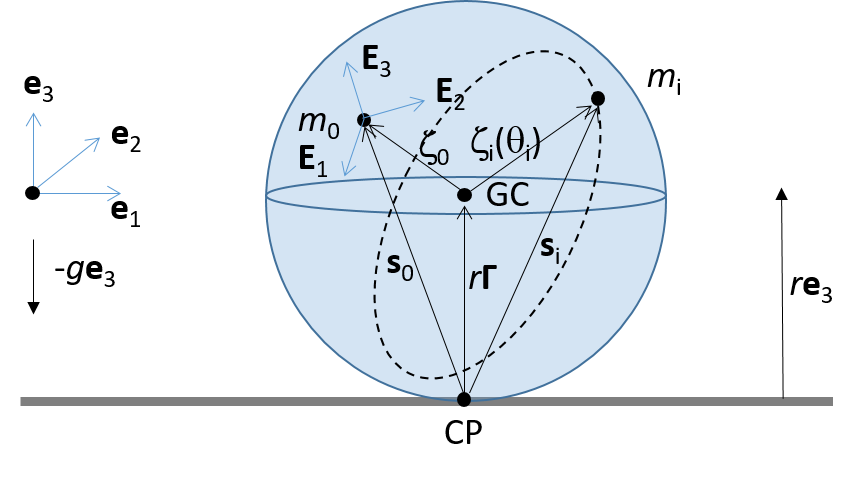
Figure 3.1: Each point mass, denoted by $m_{i}$, $1\leq i\leq n$, moves along a rail fixed inside the ball depicted here by the dashed hoop. The trajectory of the rail is denoted by $\boldsymbol{\zeta}_{i}$ and is parameterized by $\theta_{i}$.

Plugging the formulas for $\boldsymbol{\chi}_{i}$, $\dot{\boldsymbol{\chi}}_{i}$, and $\ddot{\boldsymbol{\chi}}_{i}$ given in (3.1) into the relevant formulas in Section 2 yields the equations of motion, normal force, and static friction for a rolling ball with 1-d parameterizations of the point mass trajectories. (2.20) becomes [10]

$$\begin{split}\dot{\boldsymbol{\Omega}}&=\left[\sum_{i=0}^{n}m_{i}\widehat{\mathbf{s}_{i}}^{2}-\mathbb{I}\right]^{-1}\Bigg{[}\boldsymbol{\Omega}\times\mathbb{I}\boldsymbol{\Omega}+r\tilde{\boldsymbol{\Gamma}}\times\boldsymbol{\Gamma}\\ &\hphantom{=\left[\sum_{i=0}^{n}m_{i}\widehat{\mathbf{s}_{i}}^{2}-\mathbb{I}\right]^{-1}\Bigg{[}}+\sum_{i=0}^{n}m_{i}\mathbf{s}_{i}\times\left\{g\boldsymbol{\Gamma}+\boldsymbol{\Omega}\times\left(\boldsymbol{\Omega}\times\boldsymbol{\zeta}_{i}+2\dot{\theta}_{i}\boldsymbol{\zeta}_{i}^{\prime}\right)+\dot{\theta}_{i}^{2}\boldsymbol{\zeta}_{i}^{\prime\prime}+\ddot{\theta}_{i}\boldsymbol{\zeta}_{i}^{\prime}\right\}\Bigg{]},\end{split}$$ (3.2)

(2.10) becomes

$$N=Mg+\left<\sum_{i=0}^{n}m_{i}\left[\dot{\boldsymbol{\Omega}}\times\mathbf{s}_{i}+\boldsymbol{\Omega}\times\left(\boldsymbol{\Omega}\times\boldsymbol{\zeta}_{i}+2\dot{\theta}_{i}\boldsymbol{\zeta}_{i}^{\prime}\right)+\dot{\theta}_{i}^{2}\boldsymbol{\zeta}_{i}^{\prime\prime}+\ddot{\theta}_{i}\boldsymbol{\zeta}_{i}^{\prime}\right],\boldsymbol{\Gamma}\right>-F_{\mathrm{e},3},$$ (3.3)

and (2.11) becomes

$$-f_{\mathrm{s}}\boldsymbol{\sigma}=\begin{bmatrix}\left(\Lambda\sum_{i=0}^{n}m_{i}\left[\dot{\boldsymbol{\Omega}}\times\mathbf{s}_{i}+\boldsymbol{\Omega}\times\left(\boldsymbol{\Omega}\times\boldsymbol{\zeta}_{i}+2\dot{\theta}_{i}\boldsymbol{\zeta}_{i}^{\prime}\right)+\dot{\theta}_{i}^{2}\boldsymbol{\zeta}_{i}^{\prime\prime}+\ddot{\theta}_{i}\boldsymbol{\zeta}_{i}^{\prime}\right]-\mathbf{F}_{\mathrm{e}}\right)_{12}\\ 0\end{bmatrix}.$$ (3.4)

Equations (3.2), (3.3), and (3.4) and their subsequent analysis constitute the main focus of this paper.

4 Rolling Disk with 1-d Parameterizations of the Point Mass Trajectories

Let us now consider the special case when the motion of the rolling ball is purely planar, which is the case of a rolling disk. In order to perform this two-dimensional reduction, suppose that the ball’s inertia is such that one of the ball’s principal axes, say the one labeled $\mathbf{E}_{2}$, is orthogonal to the plane containing the GC and CM. Also assume that all the point masses move along 1-d rails which lie in the plane containing the GC and CM. Moreover, suppose that the ball is oriented initially so that the plane containing the GC and CM coincides with the $\mathbf{e}_{1}$-$\mathbf{e}_{3}$ plane and that the external force $\mathbf{F}_{\mathrm{e}}$ acts in the $\mathbf{e}_{1}$-$\mathbf{e}_{3}$ plane. Then for all time, the ball will remain oriented so that the plane containing the GC and CM coincides with the $\mathbf{e}_{1}$-$\mathbf{e}_{3}$ plane and the ball will only move in the $\mathbf{e}_{1}$-$\mathbf{e}_{3}$ plane, with the ball’s rotation axis always parallel to $\mathbf{e}_{2}$. Note that the dynamics of this system are equivalent to that of the Chaplygin disk [22], equipped with point masses, rolling in the $\mathbf{e}_{1}$-$\mathbf{e}_{3}$ plane, and where the Chaplygin disk (minus the point masses) has polar moment of inertia $d_{2}$. This particular ball with this special inertia, orientation, and placement of the rails and point masses, may be referred to as the disk or the rolling disk. Figure 4.1 depicts the rolling disk.

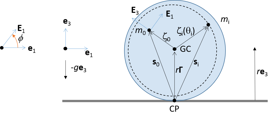
Figure 4.1: A disk of radius $r$ and mass $m_{0}$ rolls without slipping in the $\mathbf{e}_{1}$-$\mathbf{e}_{3}$ plane. $\mathbf{e}_{2}$ and $\mathbf{E}_{2}$ are directed into the page and are omitted from the figure. The disk’s center of mass is denoted by $m_{0}$. The disk’s motion is actuated by $n$ point masses, each of mass $m_{i}$, $1\leq i\leq n$, that move along rails fixed inside the disk. The point mass depicted here by $m_{i}$ moves along a circular hoop in the disk that is not centered on the disk’s geometric center (GC). The disk’s orientation is determined by $\phi$, the angle measured counterclockwise from $\mathbf{e}_{1}$ to $\mathbf{E}_{1}$.

Let $\phi$ denote the angle between $\mathbf{e}_{1}$ and $\mathbf{E}_{1}$, measured counterclockwise from $\mathbf{e}_{1}$ to $\mathbf{E}_{1}$. Thus, if $\dot{\phi}>0$, the disk rolls in the $-\mathbf{e}_{1}$ direction and $\boldsymbol{\Omega}$ has the same direction as $-\mathbf{e}_{2}$, and if $\dot{\phi}<0$, the disk rolls in the $\mathbf{e}_{1}$ direction and $\boldsymbol{\Omega}$ has the same direction as $\mathbf{e}_{2}$.

For the rolling disk with 1-d parameterizations of the point mass trajectories, (3.2) becomes [10]

$$\ddot{\phi}=\frac{\sum_{i=0}^{n}m_{i}K_{i}-rF_{\mathrm{e},1}}{d_{2}+\sum_{i=0}^{n}m_{i}\left[\left(r\sin\phi+\zeta_{i,1}\right)^{2}+\left(r\cos\phi+\zeta_{i,3}\right)^{2}\right]},$$ (4.1)

where

$$\begin{split}K_{i}&\equiv\left(g+r{\dot{\phi}}^{2}\right)\left(\zeta_{i,3}\sin\phi-\zeta_{i,1}\cos\phi\right)+\left(r\cos\phi+\zeta_{i,3}\right)\left(-2\dot{\phi}{\dot{\theta}}_{i}\zeta_{i,3}^{\prime}+{\dot{\theta}}_{i}^{2}\zeta_{i,1}^{\prime\prime}+{\ddot{\theta}}_{i}\zeta_{i,1}^{\prime}\right)\\ &\hphantom{\equiv}-\left(r\sin\phi+\zeta_{i,1}\right)\left(2\dot{\phi}{\dot{\theta}}_{i}\zeta_{i,1}^{\prime}+{\dot{\theta}}_{i}^{2}\zeta_{i,3}^{\prime\prime}+{\ddot{\theta}}_{i}\zeta_{i,3}^{\prime}\right),\end{split}$$ (4.2)

(3.3) becomes

$$\begin{split}N&=Mg+\sum_{i=0}^{n}m_{i}\Big{[}\left(-\ddot{\phi}\zeta_{i,3}-{\dot{\phi}}^{2}\zeta_{i,1}-2\dot{\phi}{\dot{\theta}}_{i}\zeta_{i,3}^{\prime}+{\dot{\theta}}_{i}^{2}\zeta_{i,1}^{\prime\prime}+{\ddot{\theta}}_{i}\zeta_{i,1}^{\prime}\right)\sin\phi\\ &\hphantom{=Mg+\sum_{i=0}^{n}m_{i}\Big{[}}+\left(\ddot{\phi}\zeta_{i,1}-{\dot{\phi}}^{2}\zeta_{i,3}+2\dot{\phi}{\dot{\theta}}_{i}\zeta_{i,1}^{\prime}+{\dot{\theta}}_{i}^{2}\zeta_{i,3}^{\prime\prime}+{\ddot{\theta}}_{i}\zeta_{i,3}^{\prime}\right)\cos\phi\Big{]}-F_{\mathrm{e},3},\end{split}$$ (4.3)

and (3.4) becomes

$$\begin{split}-f_{\mathrm{s}}\boldsymbol{\sigma}&=-\Big{\{}Mr\ddot{\phi}+\sum_{i=0}^{n}m_{i}\Big{[}\left(\ddot{\phi}\zeta_{i,3}+{\dot{\phi}}^{2}\zeta_{i,1}+2\dot{\phi}{\dot{\theta}}_{i}\zeta_{i,3}^{\prime}-{\dot{\theta}}_{i}^{2}\zeta_{i,1}^{\prime\prime}-{\ddot{\theta}}_{i}\zeta_{i,1}^{\prime}\right)\cos\phi\\ &\hphantom{=-\Big{\{}Mr\ddot{\phi}+\sum_{i=0}^{n}m_{i}\Big{[}}+\left(\ddot{\phi}\zeta_{i,1}-{\dot{\phi}}^{2}\zeta_{i,3}+2\dot{\phi}{\dot{\theta}}_{i}\zeta_{i,1}^{\prime}+{\dot{\theta}}_{i}^{2}\zeta_{i,3}^{\prime\prime}+{\ddot{\theta}}_{i}\zeta_{i,3}^{\prime}\right)\sin\phi\Big{]}+F_{\mathrm{e},1}\Big{\}}\mathbf{e}_{1}.\end{split}$$ (4.4)

Appendix A provides detailed calculations justifying how (4.3) and (4.4) follow from (3.3) and (3.4), respectively. The $\mathbf{e}_{1}$-component of $-f_{\mathrm{s}}\boldsymbol{\sigma}$ is denoted by $\pi f_{\mathrm{s}}$.

Rolling Disk with Static Internal Structure

By setting the number of point masses $n$ to 0, the dynamics and contact point forces for the rolling disk with static internal structure are readily obtained. Letting $n=0$, (4.1) simplifies to

$$\ddot{\phi}=\frac{m_{0}\left(g+r{\dot{\phi}}^{2}\right)\left(\zeta_{0,3}\sin\phi-\zeta_{0,1}\cos\phi\right)-rF_{\mathrm{e},1}}{d_{2}+m_{0}\left[\left(r\sin\phi+\zeta_{0,1}\right)^{2}+\left(r\cos\phi+\zeta_{0,3}\right)^{2}\right]},$$ (4.5)

(4.3) simplifies to

$$N=m_{0}\left[g-\left(\ddot{\phi}\zeta_{0,3}+{\dot{\phi}}^{2}\zeta_{0,1}\right)\sin\phi+\left(\ddot{\phi}\zeta_{0,1}-{\dot{\phi}}^{2}\zeta_{0,3}\right)\cos\phi\right]-F_{\mathrm{e},3},$$ (4.6)

and (4.4) simplifies to

$$-f_{\mathrm{s}}\boldsymbol{\sigma}=-\left\{m_{0}\left[r\ddot{\phi}+\left(\ddot{\phi}\zeta_{0,3}+{\dot{\phi}}^{2}\zeta_{0,1}\right)\cos\phi+\left(\ddot{\phi}\zeta_{0,1}-{\dot{\phi}}^{2}\zeta_{0,3}\right)\sin\phi\right]+F_{\mathrm{e},1}\right\}\mathbf{e}_{1}.$$ (4.7)

5 Numerical Simulations of the Dynamics of the Rolling Disk

To write the equations of motion for the rolling disk in the standard ODE form, the state of the system is defined as

$${\boldsymbol{x}}\equiv\begin{bmatrix}\boldsymbol{\theta}\\ \dot{\boldsymbol{\theta}}\\ \phi\\ \dot{\phi}\end{bmatrix},$$ (5.1)

where $\boldsymbol{\theta},\dot{\boldsymbol{\theta}}\in\mathbb{R}^{n}$ and $\phi,\dot{\phi}\in\mathbb{R}$. The ODE formulation of the rolling disk’s system dynamics defined for $a\leq t\leq b$ is

$$\dot{{\boldsymbol{x}}}=\begin{bmatrix}\dot{\boldsymbol{\theta}}\\ \ddot{\boldsymbol{\theta}}\\ \dot{\phi}\\ \ddot{\phi}\end{bmatrix}=\mathbf{f}\left(t,{\boldsymbol{x}},\boldsymbol{u}\right)\equiv\begin{bmatrix}\dot{\boldsymbol{\theta}}\\ \boldsymbol{u}\\ \dot{\phi}\\ \kappa\left(t,{\boldsymbol{x}},\boldsymbol{u}\right)\end{bmatrix},$$ (5.2)

where $\boldsymbol{u}\colon\mathbb{R}\to\mathbb{R}^{n}$ is a prescribed function of $t$ such that $\boldsymbol{u}(t)=\ddot{\boldsymbol{\theta}}(t)\in\mathbb{R}^{n}$ and $\kappa\left(t,{\boldsymbol{x}},\boldsymbol{u}\right)$ is given by the right-hand side of the formula for $\ddot{\phi}$ in (4.1). In order to simulate the rolling disk’s dynamics, (5.2) must be integrated with prescribed initial conditions at time $t=a$:

$${\boldsymbol{x}}\left(a\right)=\begin{bmatrix}\boldsymbol{\theta}(a)\\ \dot{\boldsymbol{\theta}}(a)\\ \phi(a)\\ \dot{\phi}(a)\end{bmatrix}=\begin{bmatrix}\boldsymbol{\theta}_{a}\\ {\dot{\boldsymbol{\theta}}}_{a}\\ \phi_{a}\\ \scalebox{0.75}[1.0]{$-$}\frac{{\dot{z}}_{a}}{r}\end{bmatrix}\equiv{\boldsymbol{x}}_{a}.$$ (5.3)

(5.2) and (5.3) constitute an ODE IVP. For the ODE systems considered here, one can choose $a=0$ without loss of generality; however, we shall let $a$ be arbitrary to keep our discussion general and consistent with the notation used in the literature on the numerical solution of boundary value problems [27]. Given $\phi$, the spatial $\mathbf{e}_{1}$-component $z$ of the disk’s GC and CP is $z=z_{a}-r\left(\phi-\phi_{a}\right)$, where $z_{a}$ is the spatial $\mathbf{e}_{1}$-component of the disk’s GC and CP at time $t=a$ and $\phi_{a}$ is the disk’s angle at time $t=a$.

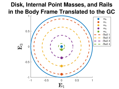
Figure 5.2: A disk of radius $r=1$ actuated by $4$ internal point masses, $m_{1}$, $m_{2}$, $m_{3}$, and $m_{4}$, each on its own circular rail of radius $r_{1}=.9$, $r_{2}=.6\overline{3}$, $r_{3}=.3\overline{6}$, and $r_{4}=.1$, respectively. The location of the disk’s CM coincides with the GC and is denoted by $m_{0}$. $m_{0}=m_{1}=m_{2}=m_{3}=m_{4}=1$ and $g=1$. The configuration at the initial time $t=0$ is shown.

Consider a rolling disk of mass $m_{0}=1$, radius $r=1$, polar moment of inertia $d_{2}=1$, and with the CM coinciding with the GC (i.e. $\boldsymbol{\zeta}_{0}=\mathbf{0}$). The disk contains $n=4$ internal point masses, each of mass $1$ so that $m_{1}=m_{2}=m_{3}=m_{4}=1$ and each located on its own concentric circle centered on the GC of radius $r_{1}=.9$, $r_{2}=.6\overline{3}$, $r_{3}=.3\overline{6}$, and $r_{4}=.1$, respectively, as shown in Figure 5.2. For $1\leq i\leq n$, the position of $m_{i}$ in the body frame centered on the GC is:

$$\boldsymbol{\zeta}_{i}\left(\theta_{i}\right)=r_{i}\begin{bmatrix}\cos\theta_{i}\\ 0\\ \sin\theta_{i}\end{bmatrix}.$$ (5.4)

The disk’s total system mass is $M=5$, and gravity is rescaled to be $g=1$. There is no external force acting on the disk’s GC so that $F_{\mathrm{e},1}=0$ in the right-hand side of (5.2). This disk’s dynamics are simulated with initial time $a=0$ and final time $b=20$, so that the simulation time interval is $\left[0,20\right]$. The parameterized acceleration of each internal point mass is a continuous approximation of a short duration unit amplitude step function:

$$u_{i}(t)=\ddot{\theta}_{i}(t)=\left(\scalebox{0.75}[1.0]{$-$}1\right)^{i}\left\{\begin{array}[]{ll}1,&0\leq t\leq.1,\\ \scalebox{0.75}[1.0]{$-$}10t+2,&.1\leq t\leq.2,\\ 0,&.2\leq t\leq 20,\end{array}\right.\quad\mbox{for}\quad 1\leq i\leq n.$$ (5.5)

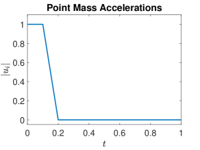
Figure 5.1: The magnitude of the parameterized acceleration, $u_{i}(t)=\ddot{\theta}_{i}(t)$, of each point mass, $1\leq i\leq n$.

The magnitudes of the functions $u_{i}(t)$ are illustrated in Figure 5.1. For each $i$, the magnitude of the parameterized acceleration $u_{i}$ is chosen to be $1$ for the short time interval $0\leq t\leq 0.1$, then decreases linearly from $1$ to $0$ for the short time interval $0.1\leq t\leq 0.2$, and finally stays constant at $0$ for the rest of time. These motions can be realized by finite, continuous forces and torques applied by the driving motors, as long as it can be assumed that the motion of the masses can be prescribed without the need to solve additional differential equations for the masses. See the discussion concerning Figure 2.1 in Section 2 and also the discussion of the same topic related to the motion of the rolling ball after (6.11) below. The parameterized accelerations $u_{i}=\ddot{\theta}_{i}$ are constructed to be continuous (instead of discontinuous) so that $\dot{\boldsymbol{\theta}}$ and $\boldsymbol{\theta}$ are differentiable. We have used these parameterized accelerations since the derivation of the equations of motion (3.2) and (4.1) assumed that $\boldsymbol{\theta}$ and $\dot{\boldsymbol{\theta}}$ are differentiable.

The rolling disk’s initial conditions are selected so that the disk starts at rest at the origin. Table 5.1 shows parameter values used in the rolling disk’s initial conditions (5.3). Since the initial orientation of the disk is $\phi_{a}=0$ and since the initial configurations of the internal point masses are given by $\boldsymbol{\theta}_{a}=\begin{bmatrix}\scalebox{0.75}[1.0]{$-$}\frac{\pi}{2}&\scalebox{0.75}[1.0]{$-$}\frac{\pi}{2}&\scalebox{0.75}[1.0]{$-$}\frac{\pi}{2}&\scalebox{0.75}[1.0]{$-$}\frac{\pi}{2}\end{bmatrix}^{\mathsf{T}}$, all the internal point masses are initially located directly below the GC, so that the disk’s total system CM is initially located below the GC. To ensure that the disk is initially at rest, ${\dot{\boldsymbol{\theta}}}_{a}=\begin{bmatrix}0&0&0&0\end{bmatrix}^{\mathsf{T}}$ and $\dot{\phi}_{a}=\scalebox{0.75}[1.0]{$-$}\frac{{\dot{z}}_{a}}{r}=0$. To ensure that the disk’s GC is initially located at the origin, $z_{a}=0$. In summary, the rolling disk’s initial conditions are

$${\boldsymbol{x}}_{a}=\begin{bmatrix}\scalebox{0.75}[1.0]{$-$}\frac{\pi}{2}&\scalebox{0.75}[1.0]{$-$}\frac{\pi}{2}&\scalebox{0.75}[1.0]{$-$}\frac{\pi}{2}&\scalebox{0.75}[1.0]{$-$}\frac{\pi}{2}&0&0&0&0&0&0\end{bmatrix}^{\mathsf{T}}.$$ (5.6)

Parameter	Value
$\boldsymbol{\theta}_{a}$	$\begin{bmatrix}\scalebox{0.75}[1.0]{$-$}\frac{\pi}{2}&\scalebox{0.75}[1.0]{$-$}\frac{\pi}{2}&\scalebox{0.75}[1.0]{$-$}\frac{\pi}{2}&\scalebox{0.75}[1.0]{$-$}\frac{\pi}{2}\end{bmatrix}^{\mathsf{T}}$
$\dot{\boldsymbol{\theta}}_{a}$	$\begin{bmatrix}0&0&0&0\end{bmatrix}^{\mathsf{T}}$
$\phi_{a}$	$0$
$\dot{\phi}_{a}$	$0$
$z_{a}$	$0$
$\dot{z}_{a}$	$0$

Table 5.1: Initial condition parameter values for the rolling disk.

The dynamics of this rolling disk are simulated by numerically integrating the ODE IVP (5.2), (5.6) via LAB R2017b and Fortran ODE-integration routines. For ODE integrators, we have used the LAB R2017b routines 45, 113, 15s, 23t, and 23tb and a LAB wrapper of the Fortran routine radau5 [28], using the default input options except for the absolute and relative error tolerances and the Jacobian. The absolute and relative error tolerances supplied to the numerical integrators are both set to $1\mathrm{e}{-12}$. The Jacobian of $\mathbf{f}$ with respect to the state ${\boldsymbol{x}}$, obtained via complex-step differentiation [29, 30, 31], is supplied to 15s, 23t, 23tb, and radau5. Since excellent agreement was observed between all the numerical integrators, only the results obtained by numerically integrating the ODE IVP (5.2), (5.6) with 45 are shown in Figures 5.3 and 5.4. We shall also note that while all the numerical integrators yielded identical results, 113 completed the numerical integration in the shortest time. Figure 5.4a shows that the magnitude of the disk’s normal force is always positive and Figure 5.4c shows that the minimum coefficient of static friction required for the disk to roll without slipping is $\hat{\mu}_{\mathrm{s}}=.2951$. The reader is referred to [32] for listings of the coefficient of static friction for pairs of materials to see which materials could be used to make this particular disk roll without slipping on the surface. For example, if the disk’s shell were made from aluminum, then it could roll without slipping on an aluminum ($\mu_{\mathrm{s}}=.42$), steel ($\mu_{\mathrm{s}}=.35$), titanium ($\mu_{\mathrm{s}}=.34$), or nickel ($\mu_{\mathrm{s}}=.33$) surface, but not on a copper ($\mu_{\mathrm{s}}=.28$), chromium ($\mu_{\mathrm{s}}=.27$), glass ($\mu_{\mathrm{s}}=.17$), or graphite ($\mu_{\mathrm{s}}=.16$) surface.

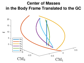
(a) Trajectories of the disk’s internal point masses and of the total system center of mass in the body frame translated to the GC.

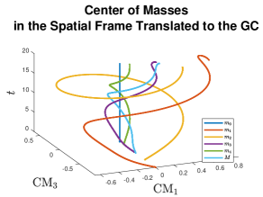
(b) Trajectories of the disk’s internal point masses and of the total system center of mass in the spatial frame translated to the GC.

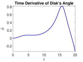
(c) Evolution of the time derivative of the disk’s rotation angle.

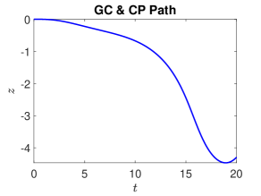
(d) Trajectory of the disk’s GC and CP.

Figure 5.3: Dynamics of the rolling disk shown in Figure 5.2 obtained by numerically integrating the ODE IVP (5.2), (5.6) with 45 over the time interval $\left[0,20\right]$. The parameterized accelerations of the internal point masses are given in (5.5).

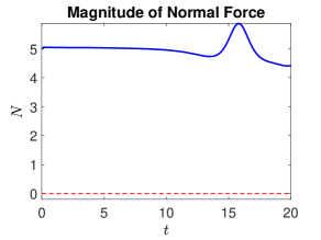
(a) The magnitude of the disk’s normal force is always positive so that the disk rolls without slipping if the coefficient of static friction exceeds $.2951$.

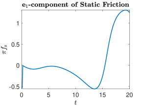
(b) $\mathbf{e}_{1}$-component of the disk’s static friction.

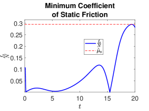
(c) Ratio of the magnitude of the static friction to the magnitude of the normal force. The minimum coefficient of static friction for the disk is $.2951$.

Figure 5.4: Contact point forces acting on the rolling disk shown in Figure 5.2 obtained by numerically integrating the ODE IVP (5.2), (5.6) with 45 over the time interval $\left[0,20\right]$. The parameterized accelerations of the internal point masses are given in (5.5). Since the magnitude of the disk’s normal force is always positive, the disk rolls without slipping if the coefficient of static friction exceeds $.2951$.

6 Numerical Simulations of the Dynamics of the Rolling Ball

To write the equations of motion for the rolling ball in the standard ordinary differential/algebraic equation (ODE/DAE) form, the state of the system is defined as

$${\boldsymbol{x}}\equiv\begin{bmatrix}\boldsymbol{\theta}\\ \dot{\boldsymbol{\theta}}\\ \mathfrak{q}\\ \boldsymbol{\Omega}\\ \boldsymbol{z}\end{bmatrix},$$ (6.1)

where $\boldsymbol{\theta},\,\dot{\boldsymbol{\theta}}\in\mathbb{R}^{n}$ encode the positions and velocities of the moving masses, the versor $\mathfrak{q}\in\mathscr{S}\cong\mathbb{S}^{3}\subset\mathbb{R}^{4}$ encodes the orientation of the rolling ball, $\boldsymbol{\Omega}\in\mathbb{R}^{3}$ is the body angular velocity, and $\boldsymbol{z}\in\mathbb{R}^{2}$ denotes the spatial $\mathbf{e}_{1}$- and $\mathbf{e}_{2}$-components of the GC and CP. Appendix D of [10] provides a brief review of quaternions and versors. Recall from [10] that given a column vector $\boldsymbol{v}\in\mathbb{R}^{3}$, $\boldsymbol{v}^{\sharp}$ is the quaternion

$$\boldsymbol{v}^{\sharp}=\begin{bmatrix}0\\ \boldsymbol{v}\end{bmatrix},$$ (6.2)

and given a quaternion $\mathfrak{p}\in\mathbb{H}$, $\mathfrak{p}^{\flat}\in\mathbb{R}^{3}$ is the column vector such that

$$\mathfrak{p}=\begin{bmatrix}p_{0}\\ \mathfrak{p}^{\flat}\end{bmatrix}.$$ (6.3)

Using a versor to parameterize the ball’s orientation implies that the state vector (6.1) consists of $2n+9$ components, whereas the state vector would be comprised of only $2n+8$ components if Euler angles were used instead. While the versor is less efficient than Euler angles at parameterizing the ball’s orientation, the versor parameterization, which is a mapping from the unit 3-sphere $\mathbb{S}^{3}$ to $SO(3)$, provides a double covering of $SO(3)$ and therefore gives a local homeomorphism about each point in $SO(3)$ [33, 34]. In contrast, the Euler angle parameterization, which is a mapping from the 3-torus $\mathbb{T}^{3}$ to $SO(3)$, is not a covering map of $SO(3)$ and therefore does not give a local homeomorphism about each point in $SO(3)$, which causes gimbal lock at those points where the parameterization is not a local homeomorphism [33, 34]. ODE and DAE formulations of the rolling ball’s system dynamics defined for $a\leq t\leq b$ are

$$\dot{{\boldsymbol{x}}}=\begin{bmatrix}\dot{\boldsymbol{\theta}}\\ \ddot{\boldsymbol{\theta}}\\ \dot{\mathfrak{q}}\\ \dot{\boldsymbol{\Omega}}\\ \dot{\boldsymbol{z}}\end{bmatrix}=\mathbf{f}\left(t,{\boldsymbol{x}},\boldsymbol{u}\right)\equiv\begin{bmatrix}\dot{\boldsymbol{\theta}}\\ \boldsymbol{u}\\ \frac{1}{2}\mathfrak{q}\boldsymbol{\Omega}^{\sharp}\\ \boldsymbol{\kappa}\left(t,{\boldsymbol{x}},\boldsymbol{u}\right)\\ \left(\left[\mathfrak{q}\boldsymbol{\Omega}^{\sharp}\mathfrak{q}^{-1}\right]^{\flat}\times r\mathbf{e}_{3}\right)_{12}\end{bmatrix}$$ (6.4)

and

$$\mathcal{M}\dot{{\boldsymbol{x}}}=\begin{bmatrix}\dot{\boldsymbol{\theta}}\\ \ddot{\boldsymbol{\theta}}\\ 0\\ {\dot{\mathfrak{q}}}^{\flat}\\ \dot{\boldsymbol{\Omega}}\\ \dot{\boldsymbol{z}}\end{bmatrix}=\mathbf{g}\left(t,{\boldsymbol{x}},\boldsymbol{u}\right)\equiv\begin{bmatrix}\dot{\boldsymbol{\theta}}\\ \boldsymbol{u}\\ \left|\mathfrak{q}\right|^{2}-1\\ \left[\frac{1}{2}\mathfrak{q}\boldsymbol{\Omega}^{\sharp}\right]^{\flat}\\ \boldsymbol{\kappa}\left(t,{\boldsymbol{x}},\boldsymbol{u}\right)\\ \left(\left[\mathfrak{q}\boldsymbol{\Omega}^{\sharp}\mathfrak{q}^{-1}\right]^{\flat}\times r\mathbf{e}_{3}\right)_{12}\end{bmatrix},$$ (6.5)

respectively, where $\boldsymbol{u}\colon\mathbb{R}\to\mathbb{R}^{n}$ is a prescribed function of $t$ such that $\boldsymbol{u}(t)=\ddot{\boldsymbol{\theta}}(t)\in\mathbb{R}^{n}$, $\boldsymbol{\kappa}\left(t,{\boldsymbol{x}},\boldsymbol{u}\right)$ is given by the right-hand side of the formula for $\dot{\boldsymbol{\Omega}}$ in (3.2), and

$$\mathcal{M}\equiv\mathrm{\textbf{diag}}\left(\begin{bmatrix}\mathbf{1}_{1\times 2n}&0&\mathbf{1}_{1\times 8}\end{bmatrix}\right)$$ (6.6)

is a diagonal DAE mass matrix. Observe that (6.5) is a semi-explicit DAE of index 1, since differentiation of the algebraic constraint $\left|\mathfrak{q}\right|^{2}-1$ with respect to time followed by using ${\dot{\mathfrak{q}}}^{\flat}=\left[\frac{1}{2}\mathfrak{q}\boldsymbol{\Omega}^{\sharp}\right]^{\flat}$ and algebraic manipulation yield the $\left(2n+1\right)^{\mathrm{st}}$ equation in (6.4), $\dot{q}_{0}=-\frac{1}{2}{\mathfrak{q}}^{\flat}\cdot\boldsymbol{\Omega}$. The reader is referred to [10] for details on the most efficient way to compute $\boldsymbol{\Gamma}\equiv\Lambda^{-1}\mathbf{e}_{3}=\left[\mathfrak{q}^{-1}\mathbf{e}_{3}^{\sharp}\mathfrak{q}\right]^{\flat}$, $\tilde{\boldsymbol{\Gamma}}\equiv\Lambda^{-1}\mathbf{F}_{\mathrm{e}}=\left[\mathfrak{q}^{-1}\mathbf{F}_{\mathrm{e}}^{\sharp}\mathfrak{q}\right]^{\flat}$, and $\boldsymbol{\omega}\equiv\left[\dot{\Lambda}\Lambda^{-1}\right]^{\vee}=\Lambda\boldsymbol{\Omega}=\left[\mathfrak{q}\boldsymbol{\Omega}^{\sharp}\mathfrak{q}^{-1}\right]^{\flat}$, which appear on the right-hand sides of (6.4) and (6.5).

In order to simulate the rolling ball’s dynamics, (6.4) or (6.5) must be integrated with prescribed initial conditions at time $t=a$:

$${\boldsymbol{x}}\left(a\right)=\begin{bmatrix}\boldsymbol{\theta}(a)\\ \dot{\boldsymbol{\theta}}(a)\\ \mathfrak{q}(a)\\ \boldsymbol{\Omega}(a)\\ \boldsymbol{z}(a)\end{bmatrix}=\begin{bmatrix}\boldsymbol{\theta}_{a}\\ {\dot{\boldsymbol{\theta}}}_{a}\\ \mathfrak{q}_{a}\\ \boldsymbol{\Omega}_{a}\\ \boldsymbol{z}_{a}\end{bmatrix}\equiv{\boldsymbol{x}}_{a}.$$ (6.7)

(6.4) and (6.7) constitute an ODE IVP, while (6.5) and (6.7) constitute a DAE IVP.

In the simulations, we consider a rolling ball of mass $m_{0}=1$, radius $r=1$, principal moments of inertia $d_{1}=.9$, $d_{2}=1$, and $d_{3}=1.1$, and with the CM shifted slightly away from the GC at $\boldsymbol{\zeta}_{0}=\begin{bmatrix}0&0&-.05\end{bmatrix}^{\mathsf{T}}$. The ball contains $n=3$ internal point masses, each of mass $1$ so that $m_{1}=m_{2}=m_{3}=1$ and each located on its own circular rail centered on the GC of radius $r_{1}=.95$, $r_{2}=.9$, and $r_{3}=.85$, respectively, oriented as shown in Figure 6.1. For $1\leq i\leq n$, the position of $m_{i}$ in the body frame centered on the GC is:

$$\boldsymbol{\zeta}_{i}\left(\theta_{i}\right)=r_{i}\mathcal{B}_{i}\left(\boldsymbol{\varsigma}\left(\mathbf{v}_{i}\right)\right)\begin{bmatrix}\cos\theta_{i}\\ 0\\ \sin\theta_{i}\end{bmatrix},$$ (6.8)

where $\mathcal{B}_{i}\left(\mathbf{n}\right)\in SO(3)$ is a rotation matrix whose columns are the right-handed orthonormal basis constructed from the unit vector $\mathbf{n}\in\mathbb{R}^{3}$ based on the algorithm given in Section 4 and Listing 2 of [35], $\boldsymbol{\varsigma}\colon\mathbb{R}^{3}\to\mathbb{R}^{3}$ maps spherical coordinates to Cartesian coordinates:

$$\boldsymbol{\varsigma}\left(\begin{bmatrix}\phi\\ \theta\\ \rho\end{bmatrix}\right)=\begin{bmatrix}\rho\cos\theta\cos\phi\\ \rho\cos\theta\sin\phi\\ \rho\sin\theta\end{bmatrix},$$ (6.9)

and

$$\mathbf{v}_{1}=\begin{bmatrix}0&0&1\end{bmatrix}^{\mathsf{T}},\quad\mathbf{v}_{2}=\begin{bmatrix}\frac{\pi}{2}&0&1\end{bmatrix}^{\mathsf{T}},\quad\mathrm{and}\quad\mathbf{v}_{3}=\begin{bmatrix}\frac{\pi}{4}&\frac{\pi}{4}&1\end{bmatrix}^{\mathsf{T}}$$ (6.10)

are spherical coordinates of unit vectors in $\mathbb{R}^{3}$. The total mass of the ball’s system is $M=4$, and gravity is rescaled to be $g=1$. There is no external force acting on the ball’s GC so that $\mathbf{F}_{\mathrm{e}}=\tilde{\boldsymbol{\Gamma}}=\mathbf{0}$ in the right-hand sides of (6.4) and (6.5). This ball’s dynamics are simulated with initial time $a=0$ and final time $b=20$, so that the simulation time interval is $\left[0,20\right]$. The parameterized acceleration of each internal point mass is a continuous approximation of a short duration unit amplitude step function:

$$u_{i}(t)=\ddot{\theta}_{i}(t)=\left\{\begin{array}[]{ll}1,&0\leq t\leq.1,\\ \scalebox{0.75}[1.0]{$-$}10t+2,&.1\leq t\leq.2,\\ 0,&.2\leq t\leq 20,\end{array}\right.\quad\mbox{for}\quad 1\leq i\leq n.$$ (6.11)

A plot of the magnitude of (6.11) is depicted in Figure 5.1. Physically, these motions of the internal masses are realized by applying finite forces and torques during the initial time interval $0\leq t\leq.1$, ramping these forces/torques to other values during the time interval $.1\leq t\leq.2$, and maintaining a uniform angular speed of the masses for all later times. If electric motors are used to actuate the masses, the actuation dynamics are coupled with the ball’s dynamics [21, 36, 37] and (6.11) is not physically realizable. In this work, we assume that the masses are actuated by stepper motors so that (6.11) is realizable, as discussed in Section 2.

The rolling ball’s initial conditions are selected so that the ball starts at rest at the origin. Table 6.2 shows parameter values used in the rolling ball’s initial conditions (6.7). The initial orientation matrix is selected to be the identity matrix so that $\mathfrak{q}_{a}=\begin{bmatrix}1&0&0&0\end{bmatrix}^{\mathsf{T}}$ and the initial configurations of the internal point masses are given by $\boldsymbol{\theta}_{a}=\begin{bmatrix}0&2.0369&0.7044\end{bmatrix}^{\mathsf{T}}$, so that the ball’s total system center of mass is initially located above the GC. These particular initial configurations of the point masses were obtained by solving a system of algebraic equations for mass positions based on the requirement that the ball’s total system center of mass be directly above or below the GC. To ensure that the ball is initially at rest, ${\dot{\boldsymbol{\theta}}}_{a}=\begin{bmatrix}0&0&0\end{bmatrix}^{\mathsf{T}}$ and $\boldsymbol{\Omega}_{a}=\begin{bmatrix}0&0&0\end{bmatrix}^{\mathsf{T}}$. To ensure that the ball’s GC is initially located at the origin, $\boldsymbol{z}_{a}=\begin{bmatrix}0&0\end{bmatrix}^{\mathsf{T}}$. In summary, the rolling ball’s initial conditions are

$${\boldsymbol{x}}_{a}=\setcounter{MaxMatrixCols}{15}\begin{bmatrix}0&2.0369&0.7044&0&0&0&1&0&0&0&0&0&0&0&0\end{bmatrix}^{\mathsf{T}}.$$ (6.12)

Parameter	Value
$\boldsymbol{\theta}_{a}$	$\begin{bmatrix}0&2.0369&.7044\end{bmatrix}^{\mathsf{T}}$
$\dot{\boldsymbol{\theta}}_{a}$	$\begin{bmatrix}0&0&0\end{bmatrix}^{\mathsf{T}}$
$\mathfrak{q}_{a}$	$\begin{bmatrix}1&0&0&0\end{bmatrix}^{\mathsf{T}}$
$\boldsymbol{\Omega}_{a}$	$\begin{bmatrix}0&0&0\end{bmatrix}^{\mathsf{T}}$
$\boldsymbol{z}_{a}$	$\begin{bmatrix}0&0\end{bmatrix}^{\mathsf{T}}$

Table 6.2: Initial condition parameter values for the rolling ball.

The dynamics of this rolling ball are simulated by numerically integrating the ODE IVP (6.4), (6.12) or the DAE IVP (6.5), (6.12). The ODE IVP (6.4), (6.12) is numerically integrated via the LAB R2017b routines 45, 113, 15s, 23t, and 23tb and a LAB wrapper of the Fortran routine radau5 [28], while the DAE IVP (6.5), (6.12) is numerically integrated via the LAB R2017b routines 15s and 23t and a LAB wrapper of the Fortran routine radau5. Except for the absolute and relative error tolerances and the Jacobian, all the numerical integrators are used with the default input options. The absolute and relative error tolerances supplied to the numerical integrators are both set to $1\mathrm{e}{-10}$. Jacobions of $\mathbf{f}$ and $\mathbf{g}$ with respect to the state ${\boldsymbol{x}}$, obtained via complex-step differentiation [29, 30, 31], are supplied to 15s, 23t, 23tb, and radau5, depending on whether the ODE or DAE IVP is numerically integrated. Since excellent agreement was observed between all the numerical integrators, only the results obtained by numerically integrating the DAE IVP (6.5), (6.12) with radau5 are shown in Figures 6.2 and 6.3. As was the case for the rolling disk, 113 completed the numerical integration of the rolling ball’s equations of motion in the shortest time. Figure 6.3a shows that the magnitude of the ball’s normal force is always positive and Figure 6.3c shows that the minimum coefficient of static friction required for the ball to roll without slipping is $\hat{\mu}_{\mathrm{s}}=.19$. The reader is referred to [32] for listings of the coefficient of static friction for pairs of materials to see which materials could be used to make this particular ball roll without slipping on the surface. Similarly to the example of the rolling disk, if the ball’s shell were made from aluminum, then it could roll without slipping on an aluminum ($\mu_{\mathrm{s}}=.42$), steel ($\mu_{\mathrm{s}}=.35$), titanium ($\mu_{\mathrm{s}}=.34$), nickel ($\mu_{\mathrm{s}}=.33$), copper ($\mu_{\mathrm{s}}=.28$), or chromium ($\mu_{\mathrm{s}}=.27$) surface, but not on a glass ($\mu_{\mathrm{s}}=.17$) or graphite ($\mu_{\mathrm{s}}=.16$) surface.

Detachment

There are three ways to numerically simulate detachment of the ball from the horizontal surface:

1. Assume perfect friction (i.e. $\mu_{\mathrm{s}}=\infty$), which is not physically possible.

2. Assume that $\mu_{\mathrm{s}}$ is finite and be able to model slipping, which we do not know how to do at this time.

3. Assume that $\mu_{\mathrm{s}}$ is finite and construct an example for which $N=f_{\mathrm{s}}=0$ at the detachment time and for which the no-slip condition $f_{\mathrm{s}}\leq\mu_{\mathrm{s}}N$ is satisfied prior to the detachment time.

Figure 6.4 illustrates the dynamics and contact point forces of a ball that detaches under the assumption of perfect friction (i.e. $\mu_{\mathrm{s}}=\infty$), where $N=0$ and $f_{\mathrm{s}}>0$ at the detachment time $t=3.7358$. This example is obtained by simulating the same ball as that depicted in Figure 6.1, with the same initial conditions as shown in Table 6.2, the same mass excitations (6.11), and the same physical parameters as described at the beginning of this section, except that the masses have been modified so that $m_{0}=m_{1}=m_{2}=.1$ and $m_{3}=60$. The ODE IVP (6.4), (6.12) is numerically integrated with 45 using the same settings as before, except that LAB ODE event location is used to stop the numerical integration when $N=0$. However, this example is unphysical since $\mu_{\mathrm{s}}$ must be finite in reality. In reality, such an example of perfect friction detachment would slip just prior to detachment as $N\searrow 0$, since $\mu_{\mathrm{s}}$ must be finite in reality. We believe that the third option is quite exceptional in practice, and we believe it would be difficult to construct such an example.

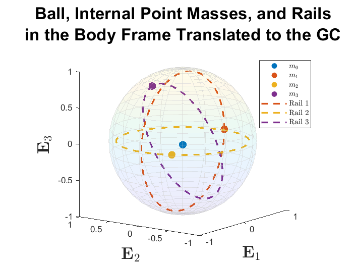
Figure 6.1: A ball of radius $r=1$ actuated by $3$ internal point masses, $m_{1}$, $m_{2}$, and $m_{3}$, each on its own circular rail of radius $r_{1}=.95$, $r_{2}=.9$, and $r_{3}=.85$, respectively. The location of the ball’s CM is shifted slightly away from the GC and is denoted by $m_{0}$. $m_{0}=m_{1}=m_{2}=m_{3}=1$ and $g=1$. The configuration at the initial time $t=0$ is shown.

(a) Trajectories of the ball’s internal point masses and of the total system center of mass in the body frame translated to the GC.

(b) Trajectories of the ball’s internal point masses and of the total system center of mass in the spatial frame translated to the GC.

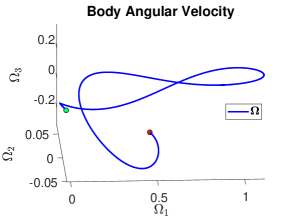
(c) Evolution of the ball’s body angular velocity.

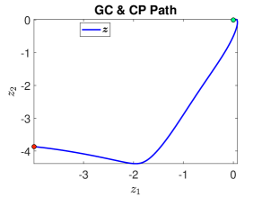
(d) Trajectory of the ball’s GC and CP.

Figure 6.2: Dynamics of the rolling ball shown in Figure 6.1 obtained by numerically integrating the DAE IVP (6.5), (6.12) with radau5 over the time interval $\left[0,20\right]$. The parameterized accelerations of the internal point masses are given in (6.11).

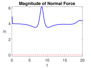
(a) The magnitude of the ball’s normal force is always positive so that the ball rolls without slipping if the coefficient of static friction exceeds $.19$.

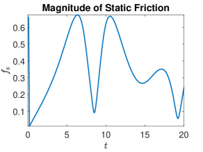
(b) Magnitude of the ball’s static friction.

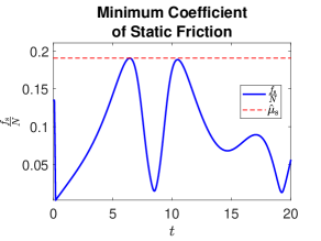
(c) Ratio of the magnitude of the static friction to the magnitude of the normal force. The minimum coefficient of static friction for the ball is $.19$.

(d) The static friction is plotted atop the trajectory of the ball’s GC and CP.

Figure 6.3: Contact point forces acting on the rolling ball shown in Figure 6.1 obtained by numerically integrating the DAE IVP (6.5), (6.12) with radau5 over the time interval $\left[0,20\right]$. The parameterized accelerations of the internal point masses are given in (6.11). Since the magnitude of the ball’s normal force is always positive, the ball rolls without slipping if the coefficient of static friction exceeds $.19$.

(a) The ball detaches at $t=3.7358$ when the magnitude of the ball’s normal force vanishes.

(b) Magnitude of the ball’s static friction.

(c) Evolution of the ball’s body angular velocity.

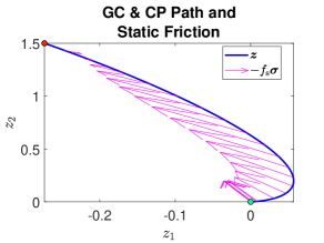
(d) The static friction is plotted atop the trajectory of the ball’s GC and CP.

Figure 6.4: Dynamics and contact point forces for the rolling ball shown in Figure 6.1 obtained by numerically integrating the ODE IVP (6.4), (6.12) with 45 over the time interval $\left[0,3.7358\right]$. The parameterized accelerations of the internal point masses are given in (6.11). Detachment occurs at the final time when $N=0$.

7 Conclusions

Newton’s laws were used to derive the equations of motion, normal force, and static friction for several cases of a ball, actuated by internal point masses, that rolls without slipping on a horizontal surface. This derivation of the equations of motion via Newton’s laws validates a previous derivation via Lagrange-d’Alembert’s principle in [10]. The dynamics of a rolling disk and ball actuated by internal point masses were simulated and the formulas for the normal force and static friction were exploited to calculate the minimum coefficient of static friction required to prevent slipping.

One may observe that the main results of the paper, equations (3.3) for the magnitude of the normal force and (3.4) for the static friction, connect the contact point forces with the dynamic variables $\dot{\boldsymbol{\Omega}}$ computed by (3.2). Thus, equations (3.3) and (3.4), in concert with the no-detachment condition (1.1) and no-slip condition (1.2), form an explicit performance envelope within which the rolling ball, actuated by moving internal point masses, must operate in order to avoid detachment and slip. Alternatively, if detachment is desired, for example, to make the ball climb up stairs or hop over an obstacle, or if slip is desired, for example, to realize a change of orientation without spatial translation of the geometric center, this performance envelope can be intentionally violated by appropriate accelerations of the masses. These questions, in part due to the complexity of the transition from slip to no-slip dynamics and vice versa, should be treated carefully in future work on the subject. We thus hope that the results presented here will be useful for further study of the dynamics and control of rolling ball robots.

Appendix A Rolling Disk Calculations

This appendix provides calculations that derive the normal force (4.3) and static friction (4.4) acting on the rolling disk. The reader is referred to Sections 2, 3, and 4 for explanations of the notation. For the rolling disk

$$\Lambda=\begin{bmatrix}\cos\phi&0&-\sin\phi\\ 0&1&0\\ \sin\phi&0&\cos\phi\end{bmatrix},$$ (A.1)

$$\boldsymbol{\Gamma}\equiv\Lambda^{-1}\mathbf{e}_{3}=\Lambda^{\mathsf{T}}\mathbf{e}_{3}=\begin{bmatrix}\sin\phi\\ 0\\ \cos\phi\end{bmatrix},\quad\boldsymbol{\Omega}\equiv\left(\Lambda^{-1}\dot{\Lambda}\right)^{\vee}=\left(\Lambda^{\mathsf{T}}\dot{\Lambda}\right)^{\vee}=\begin{bmatrix}0\\ -1\\ 0\end{bmatrix}\dot{\phi}=-\dot{\phi}\begin{bmatrix}0\\ 1\\ 0\end{bmatrix}=-\dot{\phi}\mathbf{e}_{2},$$ (A.2)

$$\boldsymbol{\zeta}_{i}=\begin{bmatrix}\zeta_{i,1}\\ 0\\ \zeta_{i,3}\end{bmatrix},\quad\boldsymbol{\zeta}_{i}^{\prime}=\begin{bmatrix}\zeta_{i,1}^{\prime}\\ 0\\ \zeta_{i,3}^{\prime}\end{bmatrix},\quad\boldsymbol{\zeta}_{i}^{\prime\prime}=\begin{bmatrix}\zeta_{i,1}^{\prime\prime}\\ 0\\ \zeta_{i,3}^{\prime\prime}\end{bmatrix},\quad\mathrm{and}\quad\mathbf{s}_{i}=r\boldsymbol{\Gamma}+\boldsymbol{\zeta}_{i}=\begin{bmatrix}r\sin\phi+\zeta_{i,1}\\ 0\\ r\cos\phi+\zeta_{i,3}\end{bmatrix}.$$ (A.3)

Therefore,

$$\dot{\boldsymbol{\Omega}}\times\mathbf{s}_{i}=\left(-\ddot{\phi}\mathbf{e}_{2}\right)\times\begin{bmatrix}r\sin\phi+\zeta_{i,1}\\ 0\\ r\cos\phi+\zeta_{i,3}\end{bmatrix}=-\ddot{\phi}\begin{bmatrix}r\cos\phi+\zeta_{i,3}\\ 0\\ -r\sin\phi-\zeta_{i,1}\end{bmatrix},$$ (A.4)

$$\boldsymbol{\Omega}\times\boldsymbol{\zeta}_{i}=\left(-\dot{\phi}\mathbf{e}_{2}\right)\times\begin{bmatrix}\zeta_{i,1}\\ 0\\ \zeta_{i,3}\end{bmatrix}=-\dot{\phi}\begin{bmatrix}\zeta_{i,3}\\ 0\\ -\zeta_{i,1}\end{bmatrix},$$ (A.5)

$$\boldsymbol{\Omega}\times\left(\boldsymbol{\Omega}\times\boldsymbol{\zeta}_{i}\right)=\left(-\dot{\phi}\mathbf{e}_{2}\right)\times-\dot{\phi}\begin{bmatrix}\zeta_{i,3}\\ 0\\ -\zeta_{i,1}\end{bmatrix}=-{\dot{\phi}}^{2}\begin{bmatrix}\zeta_{i,1}\\ 0\\ \zeta_{i,3}\end{bmatrix},$$ (A.6)

$$2\dot{\theta}_{i}\boldsymbol{\Omega}\times\boldsymbol{\zeta}_{i,1}^{\prime}=2\dot{\theta}_{i}\left(-\dot{\phi}\mathbf{e}_{2}\right)\times\begin{bmatrix}\zeta_{i,1}^{\prime}\\ 0\\ \zeta_{i,3}^{\prime}\end{bmatrix}=-2\dot{\phi}\dot{\theta}_{i}\begin{bmatrix}\zeta_{i,3}^{\prime}\\ 0\\ -\zeta_{i,1}^{\prime}\end{bmatrix},$$ (A.7)

and

$${\dot{\theta}}_{i}^{2}\boldsymbol{\zeta}_{i}^{\prime\prime}+{\ddot{\theta}}_{i}\boldsymbol{\zeta}_{i}^{\prime}=\begin{bmatrix}{\dot{\theta}}_{i}^{2}\zeta_{i,1}^{\prime\prime}+{\ddot{\theta}}_{i}\zeta_{i,1}^{\prime}\\ 0\\ {\dot{\theta}}_{i}^{2}\zeta_{i,3}^{\prime\prime}+{\ddot{\theta}}_{i}\zeta_{i,3}^{\prime}\end{bmatrix}.$$ (A.8)

Combining (A.4), (A.6), (A.7), and (A.8) yields

$$\dot{\boldsymbol{\Omega}}\times\mathbf{s}_{i}+\boldsymbol{\Omega}\times\left(\boldsymbol{\Omega}\times\boldsymbol{\zeta}_{i}+2\dot{\theta}_{i}\boldsymbol{\zeta}_{i}^{\prime}\right)+\dot{\theta}_{i}^{2}\boldsymbol{\zeta}_{i}^{\prime\prime}+\ddot{\theta}_{i}\boldsymbol{\zeta}_{i}^{\prime}=\begin{bmatrix}-r\ddot{\phi}\cos\phi-\ddot{\phi}\zeta_{i,3}-{\dot{\phi}}^{2}\zeta_{i,1}-2\dot{\phi}{\dot{\theta}}_{i}\zeta_{i,3}^{\prime}+{\dot{\theta}}_{i}^{2}\zeta_{i,1}^{\prime\prime}+{\ddot{\theta}}_{i}\zeta_{i,1}^{\prime}\\ 0\\ r\ddot{\phi}\sin\phi+\ddot{\phi}\zeta_{i,1}-{\dot{\phi}}^{2}\zeta_{i,3}+2\dot{\phi}{\dot{\theta}}_{i}\zeta_{i,1}^{\prime}+{\dot{\theta}}_{i}^{2}\zeta_{i,3}^{\prime\prime}+{\ddot{\theta}}_{i}\zeta_{i,3}^{\prime}\end{bmatrix}.$$ (A.9)

Substituting (A.9) into (3.3) and (3.4) yields (4.3) and (4.4), respectively.

Appendix B Detachment Dynamics

This appendix derives the dynamics of the ball and disk when they are detached from the surface. The reader is referred to Sections 2, 3, and 4 for explanations of the notation. Suppose that the ball is detached from the surface, so that $\mbox{z}_{\mathrm{GC},3}\geq 0$ and $N=f_{\mathrm{s}}=0$. Setting $N=f_{\mathrm{s}}=0$ in (2.5), Newton’s laws of linear motion about the ball’s CM give

$$\mathbf{0}=-Mg\mathbf{e}_{3}+\mathbf{F}_{\mathrm{e}}-\sum_{i=0}^{n}m_{i}{\ddot{\mathbf{z}}}_{i}.$$ (B.1)

For $0\leq i\leq n$,

$$\mathbf{z}_{i}=\mathbf{z}_{\mathrm{GC}}+\Lambda\boldsymbol{\chi}_{i}.$$ (B.2)

Therefore,

$${\dot{\mathbf{z}}}_{i}={\dot{\mathbf{z}}}_{\mathrm{GC}}+\Lambda\left[\boldsymbol{\Omega}\times\boldsymbol{\chi}_{i}+{\dot{\boldsymbol{\chi}}}_{i}\right]$$ (B.3)

and

$${\ddot{\mathbf{z}}}_{i}={\ddot{\mathbf{z}}}_{\mathrm{GC}}+\Lambda\left[\dot{\boldsymbol{\Omega}}\times\boldsymbol{\chi}_{i}+\boldsymbol{\Omega}\times\left(\boldsymbol{\Omega}\times\boldsymbol{\chi}_{i}+2{\dot{\boldsymbol{\chi}}}_{i}\right)+{\ddot{\boldsymbol{\chi}}}_{i}\right].$$ (B.4)

Plugging (B.4) into (B.1) gives

$$\mathbf{0}=-Mg\mathbf{e}_{3}+\mathbf{F}_{\mathrm{e}}-\sum_{i=0}^{n}m_{i}\left\{{\ddot{\mathbf{z}}}_{\mathrm{GC}}+\Lambda\left[\dot{\boldsymbol{\Omega}}\times\boldsymbol{\chi}_{i}+\boldsymbol{\Omega}\times\left(\boldsymbol{\Omega}\times\boldsymbol{\chi}_{i}+2{\dot{\boldsymbol{\chi}}}_{i}\right)+{\ddot{\boldsymbol{\chi}}}_{i}\right]\right\}.$$ (B.5)

Solving (B.5) for $\ddot{\mathbf{z}}_{\mathrm{GC}}$ gives

$$\ddot{\mathbf{z}}_{\mathrm{GC}}=\frac{1}{M}\mathbf{F}_{\mathrm{e}}-g\mathbf{e}_{3}-\frac{1}{M}\Lambda\sum_{i=0}^{n}m_{i}\left[\dot{\boldsymbol{\Omega}}\times\boldsymbol{\chi}_{i}+\boldsymbol{\Omega}\times\left(\boldsymbol{\Omega}\times\boldsymbol{\chi}_{i}+2{\dot{\boldsymbol{\chi}}}_{i}\right)+{\ddot{\boldsymbol{\chi}}}_{i}\right].$$ (B.6)

(B.1) may be rewritten as

$$\mathbf{0}=\mathbf{F}_{\mathrm{e}}-\sum_{i=0}^{n}m_{i}\left({\ddot{\mathbf{z}}}_{i}+g\mathbf{e}_{3}\right).$$ (B.7)

Multiplying both sides of (B.7) by $\Lambda^{-1}$ gives

$$\mathbf{0}=\tilde{\boldsymbol{\Gamma}}-\sum_{i=0}^{n}m_{i}\left(\Lambda^{-1}{\ddot{\mathbf{z}}}_{i}+g\boldsymbol{\Gamma}\right).$$ (B.8)

Crossing both sides of (B.8) by $\boldsymbol{\chi}_{0}$ and solving for $\tilde{\boldsymbol{\Gamma}}\times\boldsymbol{\chi}_{0}$ gives

$$\tilde{\boldsymbol{\Gamma}}\times\boldsymbol{\chi}_{0}=\sum_{i=0}^{n}m_{i}\left(\Lambda^{-1}{\ddot{\mathbf{z}}}_{i}+g\boldsymbol{\Gamma}\right)\times\boldsymbol{\chi}_{0}.$$ (B.9)

Setting $N=f_{\mathrm{s}}=0$ in (2.15), Newton’s laws of angular motion about the ball’s CM give

$$\boldsymbol{\Omega}\times\mathbb{I}\boldsymbol{\Omega}+\mathbb{I}\dot{\boldsymbol{\Omega}}=-\boldsymbol{\chi}_{0}\times\tilde{\boldsymbol{\Gamma}}-\sum_{i=1}^{n}\left(\boldsymbol{\chi}_{i}-\boldsymbol{\chi}_{0}\right)\times m_{i}\left(\Lambda^{-1}{\ddot{\mathbf{z}}}_{i}+g\boldsymbol{\Gamma}\right).$$ (B.10)

Plugging (B.9) into (B.10) gives

$$\boldsymbol{\Omega}\times\mathbb{I}\boldsymbol{\Omega}+\mathbb{I}\dot{\boldsymbol{\Omega}}=-\sum_{i=0}^{n}\boldsymbol{\chi}_{i}\times m_{i}\left(\Lambda^{-1}{\ddot{\mathbf{z}}}_{i}+g\boldsymbol{\Gamma}\right).$$ (B.11)

Multiplying both sides of (B.4) by $\Lambda^{-1}$ and using (B.6) gives

$$\Lambda^{-1}{\ddot{\mathbf{z}}}_{i}=\frac{1}{M}\tilde{\boldsymbol{\Gamma}}-g\boldsymbol{\Gamma}-\sum_{j=0}^{n}\left(\frac{m_{j}}{M}-\delta_{ij}\right)\left[\dot{\boldsymbol{\Omega}}\times\boldsymbol{\chi}_{j}+\boldsymbol{\Omega}\times\left(\boldsymbol{\Omega}\times\boldsymbol{\chi}_{j}+2{\dot{\boldsymbol{\chi}}}_{j}\right)+{\ddot{\boldsymbol{\chi}}}_{j}\right].$$ (B.12)

Plugging (B.12) into (B.11) yields

$$\boldsymbol{\Omega}\times\mathbb{I}\boldsymbol{\Omega}+\mathbb{I}\dot{\boldsymbol{\Omega}}=-\sum_{i=0}^{n}\boldsymbol{\chi}_{i}\times m_{i}\left\{\frac{1}{M}\tilde{\boldsymbol{\Gamma}}-\sum_{j=0}^{n}\left(\frac{m_{j}}{M}-\delta_{ij}\right)\left[\dot{\boldsymbol{\Omega}}\times\boldsymbol{\chi}_{j}+\boldsymbol{\Omega}\times\left(\boldsymbol{\Omega}\times\boldsymbol{\chi}_{j}+2{\dot{\boldsymbol{\chi}}}_{j}\right)+{\ddot{\boldsymbol{\chi}}}_{j}\right]\right\},$$ (B.13)

which simplifies to

$$\left[\mathbb{I}+\sum_{i=0}^{n}m_{i}\widehat{\boldsymbol{\chi}_{i}}\left\{\sum_{j=0}^{n}\left(\frac{m_{j}}{M}-\delta_{ij}\right)\widehat{\boldsymbol{\chi}_{j}}\right\}\right]\dot{\boldsymbol{\Omega}}\\ =\mathbb{I}\boldsymbol{\Omega}\times\boldsymbol{\Omega}-\sum_{i=0}^{n}m_{i}\boldsymbol{\chi}_{i}\times\left\{\frac{1}{M}\tilde{\boldsymbol{\Gamma}}-\sum_{j=0}^{n}\left(\frac{m_{j}}{M}-\delta_{ij}\right)\left[\boldsymbol{\Omega}\times\left(\boldsymbol{\Omega}\times\boldsymbol{\chi}_{j}+2{\dot{\boldsymbol{\chi}}}_{j}\right)+{\ddot{\boldsymbol{\chi}}}_{j}\right]\right\}.$$ (B.14)

Solving (B.14) for $\dot{\boldsymbol{\Omega}}$ yields

$$\dot{\boldsymbol{\Omega}}=\left[\mathbb{I}+\sum_{i=0}^{n}m_{i}\widehat{\boldsymbol{\chi}_{i}}\left\{\sum_{j=0}^{n}\left(\frac{m_{j}}{M}-\delta_{ij}\right)\widehat{\boldsymbol{\chi}_{j}}\right\}\right]^{-1}\\ \left[\mathbb{I}\boldsymbol{\Omega}\times\boldsymbol{\Omega}-\sum_{i=0}^{n}m_{i}\boldsymbol{\chi}_{i}\times\left\{\frac{1}{M}\tilde{\boldsymbol{\Gamma}}-\sum_{j=0}^{n}\left(\frac{m_{j}}{M}-\delta_{ij}\right)\left[\boldsymbol{\Omega}\times\left(\boldsymbol{\Omega}\times\boldsymbol{\chi}_{j}+2{\dot{\boldsymbol{\chi}}}_{j}\right)+{\ddot{\boldsymbol{\chi}}}_{j}\right]\right\}\right].$$ (B.15)

The detachment dynamics for the ball are given by (B.15) and (B.6).

Ball with Static Internal Structure

By setting the number of point masses $n$ to 0, the detachment dynamics for the ball with static internal structure are readily obtained. Letting $n=0$, (B.15) and (B.6) simplify to

$$\begin{split}\dot{\boldsymbol{\Omega}}&=\mathbb{I}^{-1}\left[\mathbb{I}\boldsymbol{\Omega}\times\boldsymbol{\Omega}+\tilde{\boldsymbol{\Gamma}}\times\boldsymbol{\chi}_{0}\right]\\ \ddot{\mathbf{z}}_{\mathrm{GC}}&=\frac{1}{m_{0}}\mathbf{F}_{\mathrm{e}}-g\mathbf{e}_{3}-\Lambda\left[\dot{\boldsymbol{\Omega}}\times\boldsymbol{\chi}_{0}+\boldsymbol{\Omega}\times\left(\boldsymbol{\Omega}\times\boldsymbol{\chi}_{0}\right)\right].\end{split}$$ (B.16)

Ball with 1-d Parameterizations of the Point Mass Trajectories

Plugging the formulas for $\boldsymbol{\chi}_{i}$, $\dot{\boldsymbol{\chi}}_{i}$, and $\ddot{\boldsymbol{\chi}}_{i}$ given in (3.1) into (B.15) and (B.6) yields the detachment dynamics for a ball with 1-d parameterizations of the point mass trajectories:

$$\begin{split}\dot{\boldsymbol{\Omega}}&=\left[\mathbb{I}+\sum_{i=0}^{n}m_{i}\widehat{\boldsymbol{\zeta}_{i}}\left\{\sum_{j=0}^{n}\left(\frac{m_{j}}{M}-\delta_{ij}\right)\widehat{\boldsymbol{\zeta}_{j}}\right\}\right]^{-1}\\ &\hskip 28.45274pt\left[\mathbb{I}\boldsymbol{\Omega}\times\boldsymbol{\Omega}-\sum_{i=0}^{n}m_{i}\boldsymbol{\zeta}_{i}\times\left\{\frac{1}{M}\tilde{\boldsymbol{\Gamma}}-\sum_{j=0}^{n}\left(\frac{m_{j}}{M}-\delta_{ij}\right)\left[\boldsymbol{\Omega}\times\left(\boldsymbol{\Omega}\times\boldsymbol{\zeta}_{j}+2\dot{\theta}_{j}\boldsymbol{\zeta}_{j}^{\prime}\right)+\dot{\theta}_{j}^{2}\boldsymbol{\zeta}_{j}^{\prime\prime}+\ddot{\theta}_{j}\boldsymbol{\zeta}_{j}^{\prime}\right]\right\}\right]\\ \ddot{\mathbf{z}}_{\mathrm{GC}}&=\frac{1}{M}\mathbf{F}_{\mathrm{e}}-g\mathbf{e}_{3}-\frac{1}{M}\Lambda\sum_{i=0}^{n}m_{i}\left[\dot{\boldsymbol{\Omega}}\times\boldsymbol{\zeta}_{i}+\boldsymbol{\Omega}\times\left(\boldsymbol{\Omega}\times\boldsymbol{\zeta}_{i}+2\dot{\theta}_{i}\boldsymbol{\zeta}_{i}^{\prime}\right)+\dot{\theta}_{i}^{2}\boldsymbol{\zeta}_{i}^{\prime\prime}+\ddot{\theta}_{i}\boldsymbol{\zeta}_{i}^{\prime}\right].\end{split}$$ (B.17)

Disk with 1-d Parameterizations of the Point Mass Trajectories

By using the results in Section 3.4 and Appendix C of [10] and in Appendix A, (B.17) simplifies to give the detachment dynamics for a disk with 1-d parameterizations of the point mass trajectories:

$$\begin{split}\ddot{\phi}&=\frac{\sum_{i=0}^{n}m_{i}\left[F_{\mathrm{e},1}\left(\zeta_{i,1}\sin\phi+\zeta_{i,3}\cos\phi\right)-F_{\mathrm{e},3}\left(\zeta_{i,1}\cos\phi-\zeta_{i,3}\sin\phi\right)+\sum_{j=0}^{n}\left(m_{j}-M\delta_{ij}\right)V_{ij}\right]}{Md_{2}-\sum_{i=0}^{n}m_{i}\left(m_{i}-M\right)\left(\zeta_{i,1}^{2}+\zeta_{i,3}^{2}\right)-2\sum_{i=0}^{n}\sum_{j=i+1}^{n}m_{i}m_{j}\left(\zeta_{i,1}\zeta_{j,1}+\zeta_{i,3}\zeta_{j,3}\right)}\\ \ddot{\mathbf{z}}_{\mathrm{GC}}&=\frac{1}{M}\begin{bmatrix}F_{\mathrm{e},1}-\sum_{i=0}^{n}m_{i}\left[\cos\phi\left(-\ddot{\phi}\zeta_{i,3}+Q_{i}\right)-\sin\phi\left(\ddot{\phi}\zeta_{i,1}+P_{i}\right)\right]\\ 0\\ F_{\mathrm{e},3}-Mg-\sum_{i=0}^{n}m_{i}\left[\sin\phi\left(-\ddot{\phi}\zeta_{i,3}+Q_{i}\right)+\cos\phi\left(\ddot{\phi}\zeta_{i,1}+P_{i}\right)\right]\end{bmatrix},\end{split}$$ (B.18)

where

$$\begin{split}P_{i}&\equiv-{\dot{\phi}}^{2}\zeta_{i,3}+2\dot{\phi}{\dot{\theta}}_{i}\zeta_{i,1}^{\prime}+{\dot{\theta}}_{i}^{2}\zeta_{i,3}^{\prime\prime}+{\ddot{\theta}}_{i}\zeta_{i,3}^{\prime}\\ Q_{i}&\equiv-{\dot{\phi}}^{2}\zeta_{i,1}-2\dot{\phi}{\dot{\theta}}_{i}\zeta_{i,3}^{\prime}+{\dot{\theta}}_{i}^{2}\zeta_{i,1}^{\prime\prime}+{\ddot{\theta}}_{i}\zeta_{i,1}^{\prime}\\ V_{ij}&\equiv\zeta_{i,1}P_{j}-\zeta_{i,3}Q_{j}.\end{split}$$ (B.19)

Disk with Static Internal Structure

By setting the number of point masses $n$ to 0, the detachment dynamics for the disk with static internal structure are readily obtained. Letting $n=0$, (B.18) simplifies to

$$\begin{split}\ddot{\phi}&=\frac{1}{d_{2}}\left[F_{\mathrm{e},1}\left(\zeta_{0,1}\sin\phi+\zeta_{0,3}\cos\phi\right)-F_{\mathrm{e},3}\left(\zeta_{0,1}\cos\phi-\zeta_{0,3}\sin\phi\right)\right]\\ \ddot{\mathbf{z}}_{\mathrm{GC}}&=\begin{bmatrix}\frac{F_{\mathrm{e},1}}{M}+\cos\phi\left(\ddot{\phi}\zeta_{0,3}+{\dot{\phi}}^{2}\zeta_{0,1}\right)+\sin\phi\left(\ddot{\phi}\zeta_{0,1}-{\dot{\phi}}^{2}\zeta_{0,3}\right)\\ 0\\ \frac{F_{\mathrm{e},3}}{M}-g+\sin\phi\left(\ddot{\phi}\zeta_{0,3}+{\dot{\phi}}^{2}\zeta_{0,1}\right)-\cos\phi\left(\ddot{\phi}\zeta_{0,1}-{\dot{\phi}}^{2}\zeta_{0,3}\right)\end{bmatrix}.\end{split}$$ (B.20)

References

- [1] A.V. Borisov, A.A. Kilin and I.S. Mamaev “How to Control Chaplygin’s Sphere Using Rotors” In Regular and Chaotic Dynamics 17, 2012, pp. 258–272
- [2] A.V. Borisov, A.A. Kilin and I.S. Mamaev “How to Control Chaplygin’s Sphere Using Rotors II” In Regular and Chaotic Dynamics 18, 2013, pp. 144–158
- [3] M.R. Burkhardt and J.W. Burdick “Reduced dynamical equations for barycentric spherical robots” In Robotics and Automation (ICRA), 2016 IEEE International Conference on, 2016, pp. 2725–2732 IEEE
- [4] A.A. Kilin, E.N. Pivovarova and T.B. Ivanova “Spherical robot of combined type: Dynamics and control” In Regular and Chaotic Dynamics 20.6 Springer, 2015, pp. 716–728
- [5] S. Gajbhiye and R.N. Banavar “Geometric modeling and local controllability of a spherical mobile robot actuated by an internal pendulum” In International Journal of Robust and Nonlinear Control 26.11 Wiley Online Library, 2016, pp. 2436–2454
- [6] T. Das, R. Mukherjee and H. Yuksel “Design considerations in the development of a spherical mobile robot” In Proc. 15th SPIE Annual International Symposium on Aerospace/Defense Sensing, Simulation, and Controls 4364, 2001, pp. 61–71
- [7] P. Mojabi “Introducing August: a novel strategy for an omnidirectional spherical rolling robot” In Robotics and Automation, 2002. Proceedings. ICRA’02. IEEE International Conference on 4, 2002, pp. 3527–3533 IEEE
- [8] J. Shen, D.A. Schneider and A.M. Bloch “Controllability and motion planning of a multibody Chaplygin’s sphere and Chaplygin’s top” In International Journal of Robust and Nonlinear Control 18.9 Wiley Online Library, 2008, pp. 905–945
- [9] K.I. Ilin, H.K. Moffatt and V.A. Vladimirov “Dynamics of a rolling robot” In Proceedings of the National Academy of Sciences National Academy of Sciences, 2017, pp. 12858–12863
- [10] V. Putkaradze and S.M. Rogers “On the dynamics of a rolling ball actuated by internal point masses” In Meccanica 53.15, 2018, pp. 3839–3868 DOI: 10.1007/s11012-018-0904-5
- [11] Editorial board “Editorial discussion on some papers by G.M. Rosenblat (in Russian)” In Nonlinear Dynamics 5, 2009, pp. 621–624
- [12] T.B. Ivanova and E.N. Pivovarova “Comments on the Paper by A.V. Borisov, A.A. Kilin, I.S. Mamaev ’How to Control the Chaplygin Ball Using Rotors. II”’ In Regular and Chaotic Dynamics 19, 2014, pp. 140–143
- [13] V.V. Vaskin and O.S. Naimushina “A study of the motion of axisymmetric sphere with a shifted center of mass on a rough plane (In Russian)” In Proc. Udmurt State University 2, 2012, pp. 10–17
- [14] A. Wagner et al. “Analysis of an oscillatory Painlevé–Klein apparatus with a nonholonomic constraint” In Differential Equations and Dynamical Systems 21.1-2 Springer, 2013, pp. 149–157
- [15] T.B. Ivanova and I.S. Mamaev “Dynamics of a Painleve-Appel system” In Journal of Applied Mathematics and Mechanics 80.1, 2016, pp. 7–15
- [16] A.P. Ivanov “On detachment conditions in the problem on the motion of a rigid body on a rough plane” In Regular and Chaotic Dynamics 13.4 Springer, 2008, pp. 355–368
- [17] A.P. Ivanov “Geometric representation of detachment conditions in systems with unilateral constraint” In Regular and Chaotic Dynamics 13.5 Springer, 2008, pp. 435–442
- [18] P.J. Blau “Friction science and technology: from concepts to applications” CRC press, 2008
- [19] V.V. Kozlov “On the dry-friction mechanism” In Doklady Physics 56.4, 2011, pp. 256–257 DOI: 10.1134/S1028335811040124
- [20] V.V. Kozlov “Friction by Painlevé and lagrangian mechanics” In Doklady Physics 56.6, 2011, pp. 355–358 Springer
- [21] D.V. Balandin, M.A. Komarov and G.V. Osipov “A motion control for a spherical robot with pendulum drive” In Journal of Computer and Systems Sciences International 52.4 Springer, 2013, pp. 650–663
- [22] D.D. Holm “Geometric Mechanics: Rotating, translating, and rolling”, Geometric Mechanics Imperial College Press, 2011
- [23] V. Putkaradze and S.M. Rogers “On the Optimal Control of a Rolling Ball Robot Actuated by Internal Point Masses” In arXiv preprint arXiv:1708.03829, 2017
- [24] Y. Bai, M. Svinin and M. Yamamoto “Dynamics-Based Motion Planning for a Pendulum-Actuated Spherical Rolling Robot” In Regular and Chaotic Dynamics 23.4 Springer, 2018, pp. 372–388
- [25] S.A. Chaplygin “On a motion of a heavy body of revolution on a horizontal plane” In Regular and Chaotic Dynamics 7.2 Turpion Ltd, 2002, pp. 119–130
- [26] G.M. Rozenblat “On the separation-free motions of a rigid body on a plane” In Doklady Physics 52.8, 2007, pp. 447–449 Springer
- [27] U.M. Ascher, R.M.M. Mattheij and R.D. Russell “Numerical solution of boundary value problems for ordinary differential equations” Siam, 1994
- [28] E. Hairer and G. Wanner “Solving ordinary differential equations. II, volume 14 of Springer Series in Computational Mathematics” Springer-Verlag, Berlin, 1996
- [29] W. Squire and G. Trapp “Using complex variables to estimate derivatives of real functions” In Siam Review 40.1 SIAM, 1998, pp. 110–112
- [30] J.R.R.A. Martins, P. Sturdza and J.J. Alonso “The connection between the complex-step derivative approximation and algorithmic differentiation” In AIAA paper 921, 2001, pp. 2001
- [31] J.R.R.A. Martins, P. Sturdza and J.J. Alonso “The complex-step derivative approximation” In ACM Transactions on Mathematical Software (TOMS) 29.3 ACM, 2003, pp. 245–262
- [32] “ASM Handbook, Volume 18: Friction, Lubrication, and Wear Technology”, 2017
- [33] D. Schröder “Transferring the Bearing Using a Strapdown Inertial Measurement Unit” In Applications of Geodesy to Engineering Springer, 1993, pp. 25–38
- [34] J. Stuelpnagel “On the parametrization of the three-dimensional rotation group” In SIAM review 6.4 SIAM, 1964, pp. 422–430
- [35] J.R. Frisvad “Building an orthonormal basis from a 3D unit vector without normalization” In Journal of Graphics Tools 16.3 Taylor & Francis, 2012, pp. 151–159
- [36] T.B. Ivanova and E.N. Pivovarova “Dynamics and Control of a Spherical Robot with an Axisymmetric Pendulum Actuator” In Nonlinear Dynamics & Mobile Robotics 1.1 Автономная некоммерческая организация Ижевский институт компьютерных …, 2013, pp. 71–85
- [37] T.B. Ivanova, A.A. Kilin and E.N. Pivovarova “Controlled Motion of a Spherical Robot with Feedback. II” In Journal of Dynamical and Control Systems Springer, 2017, pp. 1–16