Decoupled Classification Refinement:
Hard False Positive Suppression for Object Detection

Abstract

In this paper, we analyze failure cases of state-of-the-art detectors and observe that most hard false positives result from classification instead of localization and they have a large negative impact on the performance of object detectors. We conjecture there are three factors and prove our hypothesis with experiments: (1) Shared feature representation is not optimal due to the mismatched goals of feature learning for classification and localization; (2) large receptive field for different scales leads to redundant context information for small objects; (3) multi-task learning helps, yet optimization of the multi-task loss may result in sub-optimal for individual tasks. We demonstrate the potential of detector classification power by a simple, effective, and widely-applicable Decoupled Classification Refinement (DCR) network. In particular, DCR places a separate classification network in parallel with the localization network (base detector). With ROI Pooling placed on the early stage of the classification network, we enforce an adaptive receptive field in DCR. During training, DCR samples hard false positives from the base detector and trains a strong classifier to refine classification results. During testing, DCR refines all boxes from the base detector. Experiments show competitive results on PASCAL VOC and COCO without any bells and whistles. Our codes are available at: this link .

1 Introduction

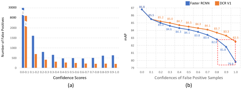
Figure 1: (a) Comparison of the number of false positives in different ranges. (b) Comparison of the mAP gains by progressively removing false positives; from right to left, the detector is performing better as false positives are removed according to their confidence scores.

Figure 2: (a) Comparison of our proposed DCR V1 and V2 with baseline in terms of different Faster RCNN series and benchmarks. (b) Speed-Accuracy comparison of DCR V1 and V2 upon Faster RCNN.

Region-based approaches with convolutional neural networks (CNNs) (Girshick et al., 2014; Girshick, 2015; Ren et al., 2015; Cai and Vasconcelos, 2018; Xu et al., 2017; Li et al., 2017b, 2018a, a; Yu et al., 2016; Hu et al., 2018; Shen et al., 2019; Wei et al., 2018) have achieved great success in object detection. Such detectors are usually built with separate classification and localization branches on top of shared feature extraction networks, and trained with multi-task loss. In particular, Faster RCNN Ren et al. (2015) learns one of the first end-to-end two-stage detector with remarkable efficiency and accuracy. Many follow-up works, such as R-FCN Dai et al. (2016), Feature Pyramid Networks (FPN) Lin et al. (2017a), Deformable ConvNets (DCN) Dai et al. (2017), have been leading popular detection benchmark in PASCAL VOC Everingham et al. (2010) and COCO Lin et al. (2014) datasets in terms of accuracy. Yet, few work has been proposed to study what is the full potential of the classification power in Faster RCNN styled detectors.

To answer this question, in this paper, we begin with investigating the key factors affecting the performance of Faster RCNN. As shown in Fig 1 (a), we conduct object detection on PASCAL VOC 2007 using Faster RCNN and count the number of false positive detections in different confidence score intervals (blue). Although only a small percentage of all false positives are predicted with high confidence scores, these samples lead to a significant performance drop in mean average precision (mAP). In particular, we perform an analysis of potential gains in mAP using Faster RCNN: As illustrated in Fig 1 (b), given the detection results from Faster RCNN and a confidence score threshold, we assume that all false positives with predicted confidence score above that threshold were classified correctly and we report the correspondent hypothesized mAP. It is evident that by correcting all false positives, Faster RCNN could, hypothetically, have achieved $86.8\%$ in mAP instead of $79.8\%$. Moreover, even if we only eliminate false positives with high confidences, as indicated in the red box, we can still improve the detection performance significantly by $3.0\%$ mAP, which is a desired yet hard-to-obtain boost for modern object detection systems.

The above observation motivates our work to alleviate the burden of false positives and improve the classification power of Faster RCNN based detectors. By scrutinizing the false positives produced by Faster RCNN, we conjecture that such errors are mainly due to three reasons: (1) Shared feature representation for both classification and localization may not be optimal for region proposal classification, the mismatched goals in feature learning lead to the reduced classification power of Faster RCNN; (2) Receptive fields in deep CNNs such as ResNet-101 He et al. (2016) are large, the whole image are usually fully covered for any given region proposals. Such large receptive fields could lead to inferior classification capacity by introducing redundant context information for small objects; and (3) Multi-task learning in general helps to improve the performance of object detectors as shown in Fast RCNN Girshick (2015) and Faster RCNN Ren et al. (2015), but the joint optimization also leads to possible sub-optimal to balance the goals of multiple tasks and could not directly utilize the full potential on individual tasks.

Following the above arguments, we propose a simple yet effective approach, named Decoupled Classification Refinement (DCR), to eliminate high-scored false positives and improve the region proposal classification results. DCR decouples the classification and localization tasks in Faster RCNN styled detectors. It takes input from a base detector, e.g. the Faster RCNN, and refine the classification results using a separate classification network which does not share features with the base detector. DCR samples hard false positives, namely the false positives with high confidence scores, from the base classifier, and then trains a stronger correctional classifier for the classification refinement. DCR is originally designed to not share any parameters with the Faster RCNN, however, we observe that sharing low-level features could speed up inference time without lossing accuracy.

Experimental results show the benefit of decoupling classification and localization tasks in object detection and, more interestingly, we find a new speed-accuracy trade-off in object detection which is controlled by the amount of features shared between classification network and localization network. Namely, we find that the less features shared between classification and localization task, the better performance a detector will achieve and, in the mean while, the slower the detector is during inference time. We hope this new trade-off can motivate the society to find new directions of improving over current objection architectures.

We conduct extensive experiments based on different Faster RCNN styled detectors (i.e. Faster RCNN, Deformable ConvNets, FPN) and benchmarks (i.e. PASCAL VOC 2007 & 2012, COCO) to demonstrate the effectiveness of our proposed simple solution in enhancing the detection performance by alleviating hard false positives. As shown in Fig 1 (a), our approach can significantly reduce the number of hard false positives and boost the detection performance by $2.7\%$ in mAP on PASCAL VOC 2007 over a strong baseline as indicated in Fig 1 (b). All of our experiment results demonstrate that our proposed DCR module can provide consistent improvements over various detection baselines, as shown in Fig 2 (a). Our contributions are fourfold:

1. We analyze the error modes of region-based object detectors and formulate the hypotheses that might cause these failure cases.

2. We propose a set of design principles to improve the classification power of Faster RCNN styled object detectors along with the DCR module based on the proposed design principles.

3. We are the first to show decoupling classification and localization helps object detection task and observe a new speed and accuracy trade-off in object detection.

4. Our DCR modules consistently bring significant performance boost to strong object detection systems on popular benchmarks and achieve competitive results. In particular, following common practice of using ResNet-101 as backbone without any bells and whistles, we achieve mAP of $84.2\%$ and $81.2\%$ on the classic PASCAL VOC 2007 and 2012 set, respectively, and $43.5\%$ on the more challenging COCO test-dev set.

This paper is an extended version of our previous work Cheng et al. (2018). In particular, we make three methodological improvements: the first one is that we propose a new DCR module that can be end-to-end trained together with the base object detector; the second one is that the proposed DCR module reduces the computation significantly without sacrificing accuracy by sharing some of the computation of regional feature at the image level; and the third one is that we come up with a inference technique that can further reduces the inference time while keeping a good speed-accuracy trade-off (Fig 2 (b)). In addition, we provide more results to demonstrate the effectiveness of our proposed method and we also perform more experiments to support our hypothesis. To justify decoupling features is important, we perform experiments to share different amount of features between classification and localization network (Table 2 (a)) and we observe that the less features shared the better the performance is (mAP increases from 78.4% to 83.0%). We further justify the importance of adaptive receptive field by placing ROI Pooling to different stages (Table 2 (b)) and we observe that the earlier ROI Pooling is placed the more adjustable receptive field can be and the better performance we get (mAP increases from 79.8% to 83.0%). These experiments also give new speed-accuracy trade-offs for object detectors.

The rest of the paper is organized as follows. In Section 3, some related works are introduced. In Section 3, we analyze problems of current object detectors. In Section 4, the details of the proposed method are described. In Section 5, we extensively perform experiments and analysis. Finally, we conclude this paper in Section 6.

2 Related Works

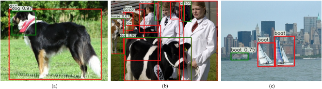
Figure 3: Demonstration of hard false positives. Results are generate by Faster RCNN with 2 fully connected layer (2fc) as detector head Ren et al. (2015); Lin et al. (2017a), red boxes are ground truth, green boxes are hard false positives with scores higher than 0.3; (a) boxes covering only part of objects with high confidences; (b) incorrect classification due to similar objects; (c) misclassified backgrounds.

Object Detection. Recent CNN based object detectors can generally be categorized into two-stage and single stage. One of the first two-stage detector is RCNN Girshick et al. (2014), where selective search Uijlings et al. (2013) is used to generate a set of region proposals for object candidates, then a deep neural network to extract feature vector of each region followed by SVM classifiers. SPPNet He et al. (2014) improves the efficiency of RCNN by sharing feature extraction stage and use spatial pyramid pooling to extract fixed length feature for each proposal. Fast RCNN Girshick (2015) improves over SPPNet by introducing an differentiable ROI Pooling operation to train the network end-to-end. Faster RCNN Ren et al. (2015) embeds the region proposal step into a Region Proposal Network (RPN) that further reduce the proposal generation time. R-FCN Dai et al. (2016) proposed a position sensitive ROI Pooling (PSROI Pooling) that can share computation among classification branch and bounding box regression branch. Deformable ConvNets (DCN) Dai et al. (2017) further add deformable convolutions and deformable ROI Pooling operations, that use learned offsets to adjust position of each sampling bin in naive convolutions and ROI Pooling, to Faster RCNN. Feature Pyramid Networks (FPN) Lin et al. (2017a) add a top-down path with lateral connections to build a pyramid of features with different resolutions and attach detection heads to each level of the feature pyramid for making prediction. Finer feature maps are more useful for detecting small objects and thus a significant boost in small object detection is observed with FPN. Most of the current state-of-the-art object detectors are two-stage detectors based of Faster RCNN, because two-stage object detectors produce more accurate results and are easier to optimize. However, two-stage detectors are slow in speed and require very large input sizes due to the ROI Pooling operation. Aimed at achieving real time object detectors, one-stage method, such as OverFeat Sermanet et al. (2013), SSD Liu et al. (2016); Fu et al. (2017) and YOLO Redmon et al. (2016); Redmon and Farhadi (2017), predict object classes and locations directly. Though single stage methods are much faster than two-stage methods, their results are inferior and they need more extra data and extensive data augmentation to get better results. Recently, there advances a new group of one-stage object detectors named anchor-free methods. One type of anchor-free methods Law and Deng (2018); Zhou et al. (2019b); Duan et al. (2019); Zhou et al. (2019a); Cheng et al. (2019b, c) are motivated by human pose estimation Cao et al. (2017); Papandreou et al. (2017); Cheng et al. (2019d). They first define “keypoints” for an object (e.g. center point Zhou et al. (2019a); Cheng et al. (2019b, c), corner point Law and Deng (2018) or extreme point Zhou et al. (2019b)) and regress to the object bounding box. Another type of anchor-free methods Tian et al. (2019); Zhu et al. (2019a) are motivated by fully convolutional networks (FCN) for semantic segmentation Long et al. (2015); Chen et al. (2018); Cheng et al. (2019a). They directly predict the bounding box on every pixel that belongs to an instance. Our paper follows the method of two-stage detectors Girshick et al. (2014); Girshick (2015); Ren et al. (2015), but with a main focus on analyzing reasons why detectors make mistakes.

Classifier Cascade. The method of classifier cascade commonly trains a stage classifier using misclassified examples from a previous classifier. This has been used a lot for object detection in the past. The Viola Jones Algorithm Viola and Jones (2004) for face detection used a hard cascades by Adaboost Freund and Schapire (1997), where a strong region classifier is built with cascade of many weak classifier focusing attentions on different features and if any of the weak classifier rejects the window, there will be no more process. Soft cascades Bourdev and Brandt (2005) improved Viola and Jones (2004) built each weak classifier based on the output of all previous classifiers. Deformable Part Model (DPM) Felzenszwalb et al. (2010) used a cascade of parts method where a root filter on coarse feature covering the entire object is combined with some part filters on fine feature with greater localization accuracy. More recently, Li et al. Li et al. (2015) proposed the Convolutional Neural Network Cascade for fast face detection. Our paper proposed a method similar to the classifier cascade idea, however, they are different in the following aspects. The classifier cascade aims at producing an efficient classifier (mainly in speed) by cascade weak but fast classifiers and the weak classifiers are used to reject examples. In comparison, our method aims at improving the overall system accuracy, where exactly two strong classifiers are cascaded and they work together to make more accurate predictions. More recent Cascade RCNN Cai and Vasconcelos (2018) proposes training object detector in a cascade manner with gradually increased IoU threshold to assign ground truth labels to align the testing metric i.e. average mAP with IOU 0.5:0.05:0.95.

3 Problems with Faster RCNN

We observe Faster RCNN produces 3 typical types of hard false positives (which may be the case for any object detector), as shown in Fig 3: (1) The classification is correct but the overlap between the predicted box and ground truth has low IoU, e.g. $<0.5$ in Fig 3 (a). This type of false negative boxes usually cover the most discriminative part and have enough information to predict the correct classes due to translation invariance. (2) Incorrect classification for predicted boxes but the IoU with ground truth are large enough, e.g. in Fig 3 (b). It happens mainly because some classes share similar discriminative parts and the predicted box does not align well with the true object and happens to cover only the discriminative parts of confusion. Another reason is that the classifier used in the detector is not strong enough to distinguish between two similar classes. (3) the detection is a “confident” background, meaning that there is no intersection or small intersection with ground truth box but classifier’s confidence score is large, e.g. in Fig 3 (c). Most of the background pattern in this case is similar to its predicted class and the classifier is too weak to distinguish. Another reason for this case is that the receptive field is fixed and it is too large for some box that it covers the actual object in its receptive field. In Fig 3 (c), the misclassified background is close to a ground truth box (the left boat), and the large receptive field (covers more than 1000 pixels in ResNet-101) might “sees” too much object features to make the wrong prediction. Given above analysis, we can conclude that the hard false positives are mainly caused by the suboptimal classifier embedded in the detector. The reasons may be that: (1) feature sharing between classification and localization, (2) detector’s receptive field does not change according to the size of objects and (3) optimizing the sum of classification loss and localization loss.

3.1 Problem with Feature Sharing

Detector backbones are usually adapted from image classification model and pre-trained on large image classification dataset. These backbones are original designed to learn scale invariant features for classification. Scale invariance is achieved by adding sub-sampling layers, e.g. max pooling, and data augmentation, e.g. random crop. Detectors place a classification branch and localization branch on top of the same backbone, however, classification needs translation invariant feature whereas localization needs translation covariant feature. During fine-tuning, the localization branch will force the backbone to gradually learn translation covariant feature, which might potentially down-grade the performance of classifier.

Ablation studies (Table 2) show that sharing less features between classification and localization branch indeed is helpful which support our hypothesis on feature sharing.

3.2 Problem with Receptive Field

Deep convolutional neural networks have fixed receptive fields. For image classification, inputs are usually cropped and resized to have fixed sizes, e.g. $224\times 224$, and network is designed to have a receptive field little larger than the input region. However, since contexts are cropped and objects with different scales are resized, the “effective receptive field” is covering the whole object.

Unlike image classification task where a single large object is in the center of a image, objects in detection task have various sizes over arbitrary locations. In Faster RCNN, the ROI pooling is introduced to crop object from 2-D convolutional feature maps to a 1-D fixed size representation for the following classification, which results in fixed receptive field (i.e. the network is attending to a fixed-size window of the input image). In such a case, objects have various sizes and the fixed receptive field will introduce different amount of context. For a small object, the context might be too large to focus on the object whereas for a large object, the receptive field might be too small that the network is looking at part of the object. Although some works introduce multi-scale features by aggregating features with different receptive field, the number of sizes is still too small comparing with the number various sizes of objects.

Recently, Deformable ConvNets V2 (DCN V2) Zhu et al. (2019b) provides a deeper analysis on the spatial support of regular convolution and deformable convolution and the authors find some interesting results that can support our hypothesis. The authors visualize the error-bounded saliency regions which can be interpreted as approximately the size of receptive field. DCN V2 observes that the receptive field of deformable convolution is changing according to the scale of objects. That is, feature within a smaller object has smaller receptive field and feature within larger object has larger receptive field. Furthermore, the receptive field of features within an object only attend to the object region. In Zhu et al. (2019b), deformable convolution learns to adapt its receptive field to mainly cover the object without introducing any background context. In contrast, the receptive field of regular convolution does not vary much and it covers much background context for small object while it only covers partial region for large objects. This observation together with the fact that deformable convolution performs better than regular convolution in Faster RCNN support our hypothesis that “adaptive” receptive field is necessary.

3.3 Problem with Optimization

Faster RCNN series are built with a feature extractor as backbone and two task-specified branches for classifying regions and the other for localizing correct locations. Denote loss functions for classification and localization as $L_{cls}$ and $L_{bbox}$, respectively. Then, the optimization of Faster RCNN series is to address a Multi-Task Learning (MTL) problem by minimizing the sum of two loss functions: $L_{detection}=L_{cls}+L_{bbox}$. However, MTL for object detection is not studied under the recent powerful classification backbones and it may be suboptimal for stronger backbones. Although it is hard to provide theoretical proof for the assumption of sub-optimal optimization in multi-task learning, some experiments results show that not using MTL may achieve better results. The purpose of this assumption is not to make any conclusion, but to motivate the society to further study multi-task learning in object detection.

4 Decoupled Classification Refinement

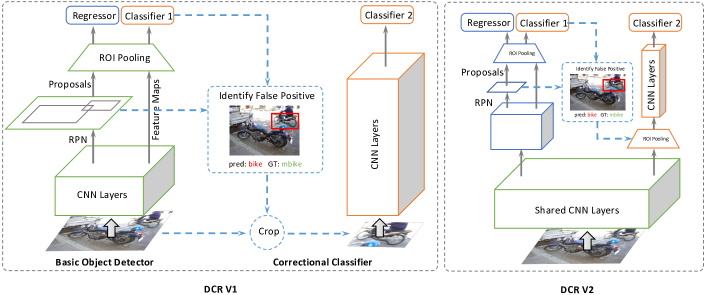
Figure 4: Left: DCR V1 module Cheng et al. (2018). Right: our proposed DCR V2 module.

In this section, we look back closely into the classic RCNN Girshick et al. (2014) method, and give an in-depth analysis of why RCNN can be used as a “complement” to improve Faster RCNN. Based on our findings, we provide a simple yet effective decoupled classification refinement (DCR) module, that can be easily added to any current state-of-the-art object detectors to provide performance improvements.

4.1 Learning from RCNN Design

We train a modified RCNN with ResNet-50 as backbone and Faster RCNN predictions as region proposals. We find that with RCNN along, the detection result is deteriorated. Since RCNN does not modify box coordinate, the inferior result means worse classification. We find that many boxes having small intersections with an object are classified as that object instead of the background which Faster RCNN predicts. Based on this finding, we hypothesize that the drawback of RCNN is mainly root from that classification model is pre-trained without awaring object location. Since ResNet-50 is trained to be translation-invariance on ImageNet in multi-crop manner, no matter how much the intersection of the crop to the object is, classifier is encouraged to predict that class. This leads to the classifier in RCNN being “too strong” for proposal classification, and this is why RCNN needs a carefully tuned sampling strategy, i.e. a ratio of 1:3 of fg to bg. Straightforwardly, we are interested whether RCNN is “strong” enough to correct hard negatives. We make a minor modification to multiply RCNN classification score with Faster RCNN classification score and observe a boost of 1.9% (from 79.8% to 81.7%)! Thus, we consider that RCNN can be seen as a compliment of Faster RCNN in the following sense: the classifier of Faster RCNN is weaker but aware of object location whereas the classifier of RCNN is unaware of object location but stronger. Based on our findings, we propose the following three principals to design a better object detector.

4.1.1 Decoupled Features

Current detectors still place classification network and localization network on the same backbone, hence we propose that classification head and localization head should not share parameter (as the analysis given in Section 3.1), resulted in a decoupled feature using pattern by RCNN.

To demonstrate it is necessary to decouple classification and localization network, we explore sharing different amount of features between classification and localization. More specifically, we use two same networks, one for classification and one for localization and experiment with the number of stages that are shared (a “stage” is a group of features that have the same resolution). Results are shown in Table 2 (a). If all features are shared, the performance is 78.4% mAP. When we share less features, the performance monotonically increases to 83.0% when only the first stage is shared.

4.1.2 Adaptive Receptive Field

The most important advantage of RCNN is that its receptive field always covers the whole ROI, i.e. the receptive field size adjusts according to the size of the object by cropping and resizing each proposal to a fixed size. We agree that context information may be important for precise detection, however, we conjuncture that different amount of context introduced by fixed receptive field might cause different performance to different sizes of objects. It leads to our last proposed principal that a detector should an adaptive receptive field that can change according to the size of objects it attends to. In this principal, the context introduced for each object should be proportional to its size, but how to decide the amount of context still remains an open question to be studied in the future. Another advantage of adaptive receptive field is that its features are well aligned to objects. Current detectors make predictions at hight-level, coarse feature maps usually having a large stride, e.g. a stride of 16 or 32 is used in Faster RCNN, due to sub-sampling operations. The sub-sampling introduces unaligned features, e.g. one cell shift on a feature map of stride 32 leads to 32 pixels shift on the image, and defects the predictions. With adaptive receptive field, the detector always attends to the entire object resulting in an aligned feature to make predictions. RCNN gives us a simple way to achieve adaptive receptive field, but how to find a more efficient way to do so remains an interesting problem needs studying.

To verify the importance of adaptive receptive field, we perform experiments by adding ROI Pooling to different stages in the parallel classification network. Results are shown in Table 2 (b). When we place the ROI Pooling at last stage, the network is less likely to adjust receptive field according to the ROI size and the performance is only 79.8%. However, as we place the ROI Pooling to earlier stages, the performance increases monotonically to 83.0%.

4.2 DCR V1: A Naïve Method

Following these principals, we propose a naïve module (DCR V1) that can be easily augmented to Faster RCNN as well as any object detector to build a stronger detector. The overall pipeline is shown in Fig 4 (left). The green part and the orange part are the original Faster RCNN and our proposed DCR module, respectively. In particular, DCR V1 mainly consists a crop-resize layer and a strong classifier. The crop-resize layer takes two inputs, the original image and boxes produced by Faster RCNN, crops boxes on the original image and feeds them to the strong classifier after resizing them to a predefined size. Region scores of DCR V1 (Classifier 2) is aggregated with region scores of Faster RCNN (Classifier 1) by element-wise product to form the final score of each region. In DCR V1, the two parts are trained separately and the scores are only combined during test time.

The classification network in DCR V1 does not share any features with the detector backbone in order to preserve the quality of classification-aimed translation invariance feature. Furthermore, there is no error propagation between the classification network in DCR V1 and the base detector, thus the optimization of one loss does not affect the other. This in turn results in a decoupled pattern where the base detector is focused more on localization (than DCR V1) whereas the DCR V1 focuses more on classification. DCR V1 introduces adaptive receptive field by resizing boxes to a predefined size. Noticed that this processing is very similar to moving an ROI Pooling from final feature maps to the image, however, it is quite different than doing ROI Pooling on feature maps. Even though the final output feature map sizes are the same, features from ROI Pooling sees larger region because objects embedded in an image has richer context. We truncated the context by cropping objects directly on the image and the network cannot see context outside object regions.

4.3 DCR V2: A Faster DCR Module

Although DCR V1 solves the problem of hard false positives, it also introduces extra computation overhead, including:

1. Cropping and resizing a large number of boxes on the original image.

2. Forward a large batch (usually 300 in Faster RCNN) of images to a deep network (a 152-layer ResNet).

The above computation overhead causes the real run time of DCR V1 module (1.3900 seconds/image) to be more than 100 times of that of the original Faster RCNN (0.0855 seconds/images). This number does not count the cropping and resizing time, which takes around 1$\sim$2 seconds per image with a sequential CPU implementation.

Inspired by He et al. (2014); Girshick (2015), we design a faster DCR module (DCR V2) that alleviates the computation overhead of DCR V1 module, shown in Fig 4 (right). That is, we solve (1) by using a highly paralleled GPU implementation of ROI Pooling and (2) by sharing part of the computation on the entire image. More specifically, we use a shared backbone network to extract high level features of the image and build the base detector and DCR V2 on top of the shared feature extractor. This design is based on the assumption that early stages of deep convolutional neural networks mainly extract low-level features (e.g. edges and textures) and we assume these low-level features can be shared among different tasks. The base detector is the same as that in the Faster RCNN and DCR V2 module is a deep convolutional classifier on regional features which are pooled by ROI Pooling.

To avoid the problem of feature sharing of classification and localization, we use a very deep residual network as the feature extractor of DCR V2. By placing this network on top of regional feature, the DCR V2 module is capable of learning translation invariance features for classifying regions. To introduce adaptive receptive field, we place the DCR V2 module at the early stage (by early stage, we mean layers that is close to input image). The early stages of network can learn texture-aware features that can be shared among different tasks as it has small stride and local receptive field. In our experiments, we also find it is beneficial to place DCR V2 module at early stage of the network.

Although sharing part of the regional feature extraction reduces the computation, we still need to process a large batch of ROIs during inference which requires a lot of memory and computation. To further reduce the inference time, we propose a simple yet efficient strategy called “top-sampling”. We find that the higher confidence score a false positive has, the larger impact it has (Fig. 1), thus we place different importance on false positives based on their confidence scores. In “top-sampling”, we only sample part of the detections whose confidence scores are within the top $p$ percent which can further reduce the inference time while preserving the accuracy. For example, if we choose $p=50\%$, then during the inference, we first score detections based on their maximum softmax scores and only pass top $50\%$ boxes into the DCR V2 module.

The “top-sampling” strategy is also based on the fact that hard false positives that cannot be suppressed by post-processing (e.g. NMS) usually have high confidence, while false positives with low confidence are less likely to be suppressed. In this way, we can achieve a speed-accuracy trade-off by “attending” to detections with high confidence scores. Experimentally, we demonstrate that processing only the top $50\%$ boxes degrades performance by less than $0.5\%$ while nearly halving the actual run time.

4.4 An AP interpretation of DCR

The success of DCR V1 Cheng et al. (2018) shows the necessity of removing false positives in object detection. However, one question in our mind is that is the effectiveness of DCR comes from model ensemble? The answer is no as we will show in Section 5. If that is the case, then what makes DCR so effective? We try to answer this question from the perspective of average precision (AP). To calculate AP, detections are first sorted according to their confidence scores which makes false positives in earlier ranking impact more than false positives in later ranking. Although DCR cannot remove all false positives, it re-ranks detections to make false positives appear later than true positive. The recent success of Mask Scoring R-CNN Huang et al. (2019) can be served as a strong evidence that ranking matters.

4.5 Training

4.5.1 Training DCR V1

Since there is no error propagates from the DCR module to Faster RCNN, we train our object detector in a two-step manner. First, we train Faster RCNN to converge. Then, we train our DCR module on mini-batches sampled from hard false positives of Faster RCNN. Parameters of DCR module are pre-trained by ImageNet dataset Deng et al. (2009). We follow the image-centric method Girshick (2015) to sample $N$ images with a total mini-batch size of $R$ boxes, i.e. $R/N$ boxes per image. We use $N=1$ and $R=32$ throughout experiments. We use a different sampling heuristic that we sample not only foreground and background boxes but also hard false positive uniformly. Because we do not want to apply any prior knowledge to impose unnecessary bias on classifier. However, we observed that boxes from the same image have little variance. Thus, we fix Batch Normalization layer with ImageNet training set statistics. The newly added linear classifier (fully connected layer) is set with 10 times of the base learning rate since we want to preserve translation invariance features learned on the ImageNet dataset.

4.5.2 Training DCR V2

We train our DCR V2 module with the base detector in an end-to-end manner. The training of the base detector is the same as Ren et al. (2015) and we mainly discuss the training of DCR V2 in detail. During training, we first sample $R$ boxes from the outputs of the bounding box regression branch in the base detector, then we use these boxes as ROIs to extract regional features in the DCR V2 module. And the training of DCR V2 module is simply minimizing the cross entropy loss. In our experiments, we follow the optimal sampling strategy and label assignment that is used for training DCR V1. The final loss term is:

$$\mathcal{L}=\mathcal{L}_{\text{RPN}}+\mathcal{L}_{\text{RCNN}}+\mathcal{L}_{\text{DCRV2}}$$

4.6 Difference with Other Cascade Methods

CRAFT Yang et al. (2016) or Cascade RCNN Cai and Vasconcelos (2018) can be categorized as using cascade classifiers to improve object detection, but they are essentially different from our approach. In particular:

1. The motivations are different. CRAFT is motivated by “divide and conquer” philosophy, it is designed to split one tasks into several small tasks. Cascade RCNN is motivated by the fact that previous training methods (use IOU 0.5 to assign foregrounds) are misaligned with testing metrics (AP with IOU 0.5-0.95). Our motivation is that Faster RCNN is making many classification errors and we want to improve it by correctly classifying those misclassified regions.

2. The architecture design principals are different. Both CRAFT and Cascade RCNN have fixed receptive field and share the backbone features. DCR uses a novel “adaptive receptive field”, we name it “adaptive” because the effective receptive field is always equal to the size of the correspondent object proposal. The classifier in DCR uses different feature from object detector.

3. The training and inference strategies are different. All three method train the cascade classifier based on the output of the previous classifier. CRAFT uses all output except background objects of the previous classifier and uses same IOU threshold (i.e. 0.5) to assign labels. Cascade RCNN uses all output but reassign foreground labels based on different IOU thresholds (i.e. 0.5, 0.6, 0.7). DCR uses only part of the previous output with a novel sampling heuristic (hard false positive sampling). In inference, both CRAFT and Cascade RCNN use prediction of the last classifier, their hypothesis is the cascade classifier is always better than the previous one. However, DCR uses both classifiers, our hypothesis is that our classifiers complement each other.

Sample method	mAP
Baseline	79.8
Random	81.8
FP Only	81.4
FP+FG	81.6
FP+BG	80.3
FP+FG+BG	82.3
RCNN-like	81.7

FP Score	mAP
Baseline	79.8
0.20	82.2
0.25	81.9
0.30	82.3
0.35	82.2
0.40	82.0

Sample size	mAP
Baseline	79.8
8 Boxes	82.0
16 Boxes	82.1
32 Boxes	82.3
64 Boxes	82.1

ROI scale	mAP	Test Time
Baseline	79.8	0.0855
$56\times 56$	80.6	0.0525
$112\times 112$	82.0	0.1454
$224\times 224$	82.3	0.5481
$320\times 320$	82.0	1.0465

(a)

(b)

(c)

(d)

DCR Depth	mAP	Test Time
Baseline	79.8	0.0855
18	81.4	0.1941
34	81.9	0.3144
50	82.3	0.5481
101	82.3	0.9570
152	82.5	1.3900

Base detector	mAP
Faster	79.8
Faster+DCR	82.3
DCN	81.4
DCN+DCR	83.2

Model capacity	mAP
Faster w/ Res101	79.8
Faster w/ Res152	80.3
Faster Ensemble	81.1
Faster w/ Res101+DCR-50	82.3

(e)

(f)

(g)

Table 1: Ablation studies results of DCR V1. Evaluate on PASCAL VOC2007 test set. Baseline is Faster RCNN with ResNet-101 as backbone. DCR V1 module uses ResNet-50. (a) Ablation study on sampling heuristics. (b) Ablation study on threshold for defining hard false positives. (c) Ablation study on sampling size. (d) Ablation study on ROI scale and test time (measured in seconds/image). (e) Ablation study on depth of DCR module and test time (measured in seconds/image). (f) DCR module with difference base detectors. Faster denotes Faster RCNN and DCN denotes Deformable Faster RCNN, both use ResNet-101 as backbone. (g) Comparison of Faster RCNN with same size as Faster RCNN + DCR.

5 Experiments

5.1 Implementation Details

5.1.1 DCR V1

We train base detectors, e.g. Faster RCNN, following their original implementations. We use default settings in 4.5 for DCR module, we use ROI size $224\times 224$ and use a threshold of 0.3 to identify hard false positives. Our DCR module is first pre-trained on the ILSVRC 2012 dataset Deng et al. (2009). In fine-tuning, we set the initial learning rate to $0.0001$ w.r.t. one GPU and weight decay of $0.0001$. We follow linear scaling rule in Goyal et al. (2017) for data parallelism on multiple GPUs and use 4 GPUs for PASCAL VOC and 8 GPUs for COCO. Synchronized SGD with momentum $0.9$ is used as optimizer. No data augmentation except horizontal flip is used.

5.1.2 DCR V2

The implementations of Faster RCNN is the same as their original ones and we will only discuss detail implementation of our DCR V2 module using a 101-layer ResNet as example.

Fig 5 (a) shows a detailed block diagram of default DCR V2 module. Follow the naming convention in mainstream frameworks’ implementation of ResNet, e.g. MXNET and PyTorch, we denote the five stages of ResNet as conv1 (the first Convolution, BatchNorm and Max Pooling that reduce input resolution by a factor of 4), Stage1 (the first residual stage containing 3 residual blocks, with output stride 4), Stage2 (the second residual stage containing 4 residual blocks, with output stride 8), Stage3 (the third residual stage containing 23 residual blocks, with output stride 16) and Stage4 (the fourth residual stage containing 3 residual blocks, with output stride 32). Following Lin et al. (2017a), we append an additional 3x3 convolution with 256 output channel after Stage4. We place the RPN at the end of Stage3 and the ROI Pooling that takes proposals from RPN as input at the end of Stage4. For the RCNN-head, we follow Lin et al. (2017a) to use two MLP with 1024 hidden layers followed by a classification branch and a bounding box regression branch. To construct the DCR V2 module, we place another ROI Pooling at the end of Stage1 that takes detections of RCNN-head as ROI input. On top of the ROI Pooling, we simply copy Stage2, Stage3, Stage4 of ResNet and add a global average pooling followed with a linear classifier. We initialize both Faster RCNN and DCR V2 module with same ImageNet pretrained weights.

We use an initial learning rate of 0.0005 and a batchsize of 1 for each GPU. The weight decay is set to 0.0005 and momentum is set to 0.9. We only use horizontal flip during training.

DCR V2 Stage	mAP	Test Time
Baseline	79.8	0.0855
Stage 4	78.4	0.0945
Stage 3	80.0	0.1543
Stage 2	82.8	0.6540
Stage 1	83.0	0.7929
Stage 0 (DCR V1)	82.3	0.9570

ROIPooling Stage	mAP	Test Time
Baseline	79.8	0.0855
Stage 3 (after DCR V2)	79.8	0.1474
Stage 2	80.7	0.2027
Stage 1	82.9	0.6590
Stage 0 (before DCR V2)	83.0	0.7929

top-$p$	mAP	Test Time
DCR V1	82.3	0.9570
100%	83.0	0.7929
75%	82.9	0.6323
50%	82.8	0.4653
25%	81.9	0.3015
0%	80.2	0.0855

(a)

(b)

(c)

Table 2: Ablation studies results of DCR V2 Module on Pascal VOC. Evaluate on PASCAL VOC2007 test set. Baseline is Faster RCNN with ResNet-101 as backbone. (a) Ablation study on the amount of feature sharing by adding DCR V2 branch after different stages in ResNet-101 backbone, ROI Pooling is placed before DCR V2 module. (b) Ablation study on adaptive receptive field by placing ROI Pooling after different stages of DCR V2 module, DCR V2 module is placed after Stage 1 of ResNet-101. (c) DCR V2 Top-Sampling during inference. Baseline model is Faster RCNN with ResNet-101 backbone. For the DCR V2 module, we place it at the end of Stage 1. The speed is measured on a single NVIDIA GTX 1080 TI.

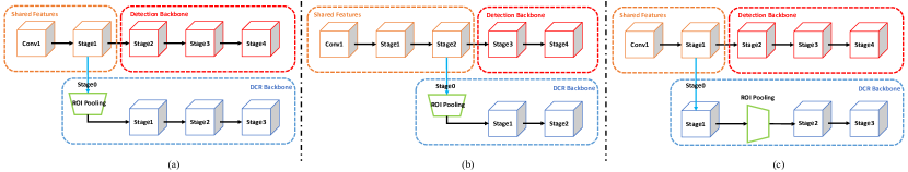
Figure 5: Illustration of ablation studies performed on DCR V2. For simplicity, detection head including RPN, ROI Pooling, cls and bbox regression are ignored. (a) Our default DCR V2 structure. (b) Ablation study on the amount of features to share. This is an example when DCR V2 is connected after Stage2 of ResNet with mAP 82.8%. (c) Ablation study on adaptive receptive field of DCR V2. This is and example when ROI Pooling is placed after Stage1 of DCR V2 with mAP 82.9%.

Ablation Settings	AP	$\text{AP}_{50}$	$\text{AP}_{75}$	$\text{AP}_{\text{S}}$	$\text{AP}_{\text{M}}$	$\text{AP}_{\text{L}}$
(a) Sampling Methods:
Baseline	25.5	44.7	26.0	6.9	26.8	42.7
Random	31.3	54.1	32.3	12.1	34.3	49.2
RCNN-like	31.5	53.8	32.4	12.7	34.2	49.5
DCR V1-like	31.4	54.2	32.0	12.6	34.2	48.8
(b) Ensemble Methods:
RCNN	15.4	42.3	7.3	8.5	20.4	21.8
Faster	25.5	44.7	26.0	6.9	26.8	42.7
{Faster, RCNN}	16.4	43.7	8.5	8.9	21.8	23.1
Faster + RCNN	28.4	51.3	28.3	11.1	30.6	45.8
DCR V2	31.4	54.2	32.0	12.6	34.2	48.8
(c) Bbox Regression:
Baseline	25.5	44.7	26.0	6.9	26.8	42.7
DCR V2 w/ bbox reg	31.2	53.9	31.9	12.3	34.3	48.4
DCR V2 w/o bbox reg	31.4	54.2	32.0	12.6	34.2	48.8
(d) Score Fusion Methods:
Baseline	25.5	44.7	26.0	6.9	26.8	42.7
DCR V2 score only	28.9	50.4	29.2	12.1	31.7	44.9
DCR V2 + Faster, multiply	31.4	54.2	32.0	12.6	34.2	48.8
DCR V2 + Faster, average	31.6	54.2	32.3	13.3	34.4	48.7

Table 3: Ablation studies results of DCR V2 Module on COCO. Evaluate on COCO2017 val set. Baseline is Faster RCNN with ResNet-50 as backbone. (a) Ablation study on sampling method. (b) Ablation study on ensemble RCNN with Faster RCNN. (c) Ablation study on adding bbox regression to DCR. (d) Ablation study on score fusion method

5.2 Ablation Studies of DCR V1

We comprehensively evaluate our method on the PASCAL VOC detection benchmark Everingham et al. (2010). We use the union of VOC 2007 trainval and VOC 2012 trainval as well as their horizontal flip as training data and evaluate results on the VOC 2007 test set. We primarily evaluate the detection mAP with IoU 0.5 (mAP@0.5). Unless otherwise stated, all ablation studies are performed with ResNet-101 for Faster RCNN, ResNet-50 as classifier for our DCR V1 module and ResNet-101 for DCR V2 module.

5.2.1 Ablation study on sampling heuristic

We compare results with different sampling heuristic in training DCR module:

• random sample: a minibatch of ROIs are randomly sampled for each image

• hard false positive only: a minibatch of ROIs that are hard positives are sampled for each image

• hard false positive and background: a minibatch of ROIs that are either hard positives or background are sampled for each image

• hard false positive and foreground: a minibatch of ROIs that are either hard positives or foreground are sampled for each image

• hard false positive, background and foreground: the difference with random sample heuristic is that we ignore easy false positives during training.

• RCNN-like: we follow the Fast RCNN’s sampling heuristic, we sample two images per GPU and 64 ROIs per image with fg:bg=1:3.

Results are shown in Table 1 (a). We find that the result is insensitive to sampling heuristic. Even with random sampling, an improvement of 2.0% in mAP is achieved. With only hard false positive, the DCR achieves an improvement of 1.6% already. Adding foreground examples only further gains a 0.2% increase. Adding background examples to false negatives harms the performance by a large margin of 1.1%. We hypothesize that this is because comparing to false positives, background examples dominating in most images results in a classifier bias to predicting background. This finding demonstrate the importance of hard negative in DCR training. Unlike RCNN-like detectors, we do not make any assumption of the distribution of hard false positives, foregrounds and backgrounds. To balance the training of classifier, we simply uniformly sample from the union set of hard false positives, foregrounds and backgrounds. This uniform sample heuristic gives the largest gain of 2.5% mAP. We also compare our training with RCNN-like training. Training with RCNN-like sampling heuristic with fg:bg=1:3 only gains a margin of 1.9%.

5.2.2 Ablation study on other hyperparameters

We compare results with different threshold for defining hard false positive: [0.2, 0.25, 0.3, 0.35, 0.4]. Results are shown in Table 1 (b). We find that the results are quite insensitive to threshold of hard false positives and we argue that this is due to our robust uniform sampling heuristic. With hard false positive threshold of 0.3, the performance is the best with a gain of 2.5%.

We also compare the influence of size of sampled RoIs during training: [8, 16, 32, 64]. Results are shown in Table 1 (c). Surprisingly, the difference of best and worst performance is only 0.3%, meaning our method is highly insensitive to the sampling size. With smaller sample size, the training is more efficient without severe drop in performance.

5.2.3 Speed and accuracy trade-off

There are in general two ways to reduce inference speed, one is to reduce the size of input and the other one is to reduce the depth of the network. We compare 4 input sizes: $56\times 56$, $112\times 112$, $224\times 224$, $320\times 320$ as well as 5 depth choices: 18, 34, 50, 101, 152 and their speed. Results are shown in Table 1 (d) and (e). The test speed is linearly related to the area of input image size and there is a severe drop in accuracy if the image size is too small, e.g. $56\times 56$. For the depth of classifier, deeper model results in more accurate predictions but also more test time. We also notice that the accuracy is correlated with the classification accuracy of classification model, which can be used as a guideline for selecting DCR module.

5.2.4 Generalization to more advanced object detectors

We evaluate the DCR V1 module on Faster RCNN and advanced Deformable Convolution Nets (DCN) Dai et al. (2017). Results are shown in Table 1 (f). Although DCN is already among one of the most accurate detectors, its classifier still produces hard false positives and our proposed DCR module is effective in eliminating those hard false positives. More results of DCR V2 on advanced detectors are shown in Table 4, 5, 6 and 7.

5.2.5 Where is the gain coming from?

One interesting question is where the accuracy gain comes from. Since we add a large convolutional network on top of the object detector, does the gain simply comes from more parameters? Or, is DCR an ensemble of two detectors? To answer this question, we compare the results of Faster RCNN with ResNet-152 as backbone (denoted Faster-152) and Faster RCNN with ResNet-101 backbone + DCR-50 (denoted Faster-101+DCR-50) and results are shown in Table 1 (g). Since the DCR module is simply a classifier, the two network have approximately the same number of parameters. However, we only observe a marginal gain of 0.5% with Faster-152 while our Faster-101+DCR-50 has a much larger gain of 2.5%. To show DCR is not simply then ensemble to two Faster RCNNs, we further ensemble Faster RCNN with ResNet-101 and ResNet-152 and the result is 81.1% which is still 1.1% worse than our Faster-101+DCR-50 model. This means that the capacity does not merely come from more parameters or ensemble of two detectors.

5.3 Ablation Studies of DCR V2

5.3.1 Ablation study on general design

We perform two ablation studies to validate general design choices for our DCR V2 module on Pascal VOC dataset: 1. after which stage to add DCR V2 module in the backbone? 2. where to add ROI Pooling to extract regional feature in the DCR V2 module? Results are shown in Table 2 (a) and (b).

We experiment on adding DCR V2 after Stage1, Stage2, Stage3, Stage4 in ResNet-101 to study the effect of feature sharing between Faster RCNN and DCR V2, and we simply use the remaining stage(s) that are not shared for DCR V2 module (Fig 5 (b)). In this case, ROI Pooling for DCR V2 is placed before DCR V2 module, i.e. DCR V2 module acts directly on the regional feature. As we place DCR V2 to earlier stages, we let Faster RCNN share less features with DCR V2 module and we observe an increase in the performance (mAP is increased from 78.4 to 83.0 as we place DCR V2 from Stage4 to Stage1). However, the inference time increases as expected. These results are consistent with our hypothesis in Section 3.1 that feature sharing between classification and localization might be harmful.

When the position of DCR V2 module is fixed (after Stage1 of the ResNet), we also explore the effect of ROI Pooling position within DCR V2 (Fig 5 (c)). The position of ROI Pooling decides a trade-off between computing regional feature and image-level feature. If we place ROI Pooling at Stage3 (the last stage) of DCR V2 (after the module), all features are computed at image level and the mAP is only 79.8. If we place ROI Pooling at Stage0 (before DCR V2 module), then all features of DCR V2 are computed at ROI level, the mAP is 83.0. This results are consistent with our hypothesis in Section 3.2 that the model should have adaptive receptive field, which means, placing ROI Pooling at earlier stage is beneficial.

5.3.2 Speed and accuracy trade-off

Results of our DCR V2 with different running times are shown in Table 2 (c). We evaluate the running time with DCR V2 after Stage1 on a single NVIDIA GTX 1080 TI GPU. Comparing with DCR V1 which has a run time of 1.3900 seconds/image, DCR V2 only requires 0.7929 seconds/image to get even better performance (+0.5% mAP) which is 1.75 times faster than DCR V1. If we use the “top-sampling” strategy to only sample top $50\%$ of the detections, the run time becomes 0.4653 seconds/image with a degradation of 0.2% in mAP, which is 3 times faster than DCR V1 and 1.7 times faster than DCR V2 with out sampling. Moreover, as mentioned earlier, the actual run time is much longer than 1.3900 seconds/image as we do not count the running time to crop and resize 300 images on the original image. That is, DCR V2 has a much better speed/accuracy trade-off over DCR V1.

Method	mAP	aero	bike	bird	boat	bottle	bus	car	cat	chair	cow	table	dog	horse	mbike	person	plant	sheep	sofa	train	tv
Faster He et al. (2016)	76.4	79.8	80.7	76.2	68.3	55.9	85.1	85.3	89.8	56.7	87.8	69.4	88.3	88.9	80.9	78.4	41.7	78.6	79.8	85.3	72.0
R-FCN Dai et al. (2016)	80.5	79.9	87.2	81.5	72.0	69.8	86.8	88.5	89.8	67.0	88.1	74.5	89.8	90.6	79.9	81.2	53.7	81.8	81.5	85.9	79.9
SSD Liu et al. (2016); Fu et al. (2017)	80.6	84.3	87.6	82.6	71.6	59.0	88.2	88.1	89.3	64.4	85.6	76.2	88.5	88.9	87.5	83.0	53.6	83.9	82.2	87.2	81.3
DSSD Fu et al. (2017)	81.5	86.6	86.2	82.6	74.9	62.5	89.0	88.7	88.8	65.2	87.0	78.7	88.2	89.0	87.5	83.7	51.1	86.3	81.6	85.7	83.7
Faster (2fc)	79.8	79.6	87.5	79.5	72.8	66.7	88.5	88.0	88.9	64.5	84.8	71.9	88.7	88.2	84.8	79.8	53.8	80.3	81.4	87.9	78.5
Faster-DCR V1	82.5	80.5	89.2	80.2	75.1	74.8	79.8	89.4	89.7	70.1	88.9	76.0	89.5	89.9	86.9	80.4	57.4	86.2	83.5	87.2	85.3
Faster-DCR V2	83.0	87.7	88.3	80.9	77.1	73.6	90.0	89.1	90.2	69.5	89.0	76.1	89.6	90.0	88.6	80.6	56.2	86.1	84.3	88.2	85.7
DCN (2fc)	81.4	83.9	85.4	80.1	75.9	68.8	88.4	88.6	89.2	68.0	87.2	75.5	89.5	89.0	86.3	84.8	54.1	85.2	82.6	86.2	80.3
DCN-DCR V1	84.0	89.3	88.7	80.5	77.7	76.3	90.1	89.6	89.8	72.9	89.2	77.8	90.1	90.0	87.5	87.2	58.6	88.2	84.3	87.5	85.0
DCN-DCR V2	84.2	90.2	89.0	80.7	77.7	75.4	89.5	89.6	90.5	72.2	89.1	80.8	90.3	90.1	87.1	87.6	58.9	86.4	84.9	88.2	87.0

Table 4: PASCAL VOC2007 test detection results.

Method	mAP	aero	bike	bird	boat	bottle	bus	car	cat	chair	cow	table	dog	horse	mbike	person	plant	sheep	sofa	train	tv
Faster He et al. (2016)	73.8	86.5	81.6	77.2	58.0	51.0	78.6	76.6	93.2	48.6	80.4	59.0	92.1	85.3	84.8	80.7	48.1	77.3	66.5	84.7	65.6
R-FCN Dai et al. (2016)	77.6	86.9	83.4	81.5	63.8	62.4	81.6	81.1	93.1	58.0	83.8	60.8	92.7	86.0	84.6	84.4	59.0	80.8	68.6	86.1	72.9
SSD Liu et al. (2016); Fu et al. (2017)	79.4	90.7	87.3	78.3	66.3	56.5	84.1	83.7	94.2	62.9	84.5	66.3	92.9	88.6	87.9	85.7	55.1	83.6	74.3	88.2	76.8
DSSD Fu et al. (2017)	80.0	92.1	86.6	80.3	68.7	58.2	84.3	85.0	94.6	63.3	85.9	65.6	93.0	88.5	87.8	86.4	57.4	85.2	73.4	87.8	76.8
Faster (2fc)	77.3	87.3	82.6	78.8	66.8	59.8	82.5	80.3	92.6	58.8	82.3	61.4	91.3	86.3	84.3	84.6	57.3	80.9	68.3	87.5	71.4
Faster-DCR V1	79.9	89.1	84.6	81.6	70.9	66.1	84.4	83.8	93.7	61.5	85.2	63.0	92.8	87.1	86.4	86.3	62.9	84.1	69.6	87.8	76.9
Faster-DCR V2	79.9	88.0	86.2	81.2	70.5	64.0	83.8	83.9	94.2	63.1	86.0	62.9	92.9	88.1	88.4	86.4	61.5	84.5	70.9	86.4	74.7
DCN (2fc)	79.4	87.9	86.2	81.6	71.1	62.1	83.1	83.0	94.2	61.0	84.5	63.9	93.1	87.9	87.2	86.1	60.4	84.0	70.5	89.0	72.1
DCN-DCR V1	81.2	89.6	86.7	83.8	72.8	68.4	83.7	85.0	94.5	64.1	86.6	66.1	94.3	88.5	88.5	87.2	63.7	85.6	71.4	88.1	76.1
DCN-DCR V2	81.1	89.3	88.5	83.9	73.8	66.3	84.0	85.0	94.2	64.0	85.5	67.1	92.8	89.0	88.0	87.4	63.3	85.2	71.5	88.7	75.1

Table 5: PASCAL VOC2012 test detection results.

Method	Backbone	AP	$\text{AP}_{50}$	$\text{AP}_{75}$	$\text{AP}_{\text{S}}$	$\text{AP}_{\text{M}}$	$\text{AP}_{\text{L}}$
Faster (2fc)	ResNet-101	30.0	50.9	30.9	9.9	33.0	49.1
Faster-DCR V1	ResNet-101 + ResNet-152	33.1	56.3	34.2	13.8	36.2	51.5
Faster-DCR V2	ResNet-101	33.6	56.7	34.7	13.5	37.1	52.2
DCN (2fc)	ResNet-101	34.4	53.8	37.2	14.4	37.7	53.1
DCN-DCR V1	ResNet-101 + ResNet-152	37.2	58.6	39.9	17.3	41.2	55.5
DCN-DCR V2	ResNet-101	37.5	58.6	40.1	17.2	42.0	55.5
FPN	ResNet-101	38.2	61.1	41.9	21.8	42.3	50.3
FPN-DCR V1	ResNet-101 + ResNet-152	40.2	63.8	44.0	24.3	43.9	52.6
FPN-DCR V2	ResNet-101	40.3	62.9	43.7	24.3	44.6	52.7
FPN-DCN	ResNet-101	41.4	63.5	45.3	24.4	45.0	55.1
FPN-DCN-DCR V1	ResNet-101 + ResNet-152	42.6	65.3	46.5	26.4	46.1	56.4
FPN-DCN-DCR V2	ResNet-101	42.8	65.1	46.8	27.1	46.6	56.1

Table 6: COCO2017 val detection results.

Method	Backbone	AP	$\text{AP}_{50}$	$\text{AP}_{75}$	$\text{AP}_{\text{S}}$	$\text{AP}_{\text{M}}$	$\text{AP}_{\text{L}}$
Mask RCNN ICCV2017 He et al. (2017)	ResNeXt-101-FPN Xie et al. (2017)	39.8	62.3	43.4	22.1	43.2	51.2
RetinaNet ICCV2017 Lin et al. (2017b)	ResNeXt-101-FPN	40.8	61.1	44.1	24.1	44.2	51.2
Relation Net CVPR2018 Hu et al. (2018)	ResNet-101	39.0	58.6	42.9	-	-	-
Cascade RCNN CVPR2018 Cai and Vasconcelos (2018)	ResNet-101-FPN	42.8	62.1	46.3	23.7	45.5	55.2
SNIP CVPR2018 Singh and Davis (2018)	ResNet-101	44.4	66.2	49.9	27.3	47.4	56.9
DetNet ECCV2018 Li et al. (2018b)	DetNet-59-FPN	40.3	62.1	43.8	23.6	42.6	50.0
CornerNet ECCV2018 Law and Deng (2018)	Hourglass-104	40.5	56.5	43.1	19.4	42.7	53.9
IOU-Net ECCV2018 Jiang et al. (2018)	ResNet-101-FPN	40.6	59.0	-	-	-	-
ExtremeNet CVPR2019 Zhou et al. (2019b)	Hourglass-104	40.2	55.5	43.2	20.4	43.2	53.1
FSAF CVPR2019 Zhu et al. (2019a)	ResNeXt-64x4d-101-FPN	42.9	63.8	46.3	26.6	46.2	52.7
FCOS ICCV2019 Tian et al. (2019)	ResNeXt-64x4d-101-FPN	43.2	62.8	46.6	26.5	46.2	53.3
CenterNet511 ICCV2019 Duan et al. (2019)	Hourglass-104	44.9	62.4	48.1	25.6	47.4	57.4
Faster (2fc)	ResNet-101	30.5	52.2	31.8	9.7	32.3	48.3
Faster-DCR V1	ResNet-101 + ResNet-152	33.9	57.9	35.3	14.0	36.1	50.8
Faster-DCR V2	ResNet-101	34.3	57.7	35.8	13.8	36.7	51.1
DCN (2fc)	ResNet-101	35.2	55.1	38.2	14.6	37.4	52.6
DCN-DCR V1	ResNet-101 + ResNet-152	38.1	59.7	41.1	17.9	41.2	54.7
DCN-DCR V2	ResNet-101	38.2	59.7	41.2	17.3	41.7	54.6
FPN	ResNet-101	38.8	61.7	42.6	21.9	42.1	49.7
FPN-DCR V1	ResNet-101 + ResNet-152	40.7	64.4	44.6	24.3	43.7	51.9
FPN-DCR V2	ResNet-101	40.8	63.6	44.5	24.3	44.3	52.0
FPN-DCN	ResNet-101	41.7	64.0	45.9	23.7	44.7	53.4
FPN-DCN-DCR V1	ResNet-101 + ResNet-152	43.1	66.1	47.3	25.8	45.9	55.3
FPN-DCN-DCR V2	ResNet-101	43.5	65.9	47.6	25.8	46.6	55.9

Table 7: COCO test-dev detection results. We only report results with single-scale test for a fair comparison.

5.3.3 More ablation studies on COCO

To help us better understand why DCR V2 works well, we perform more ablation studies on COCO using ResNet-50 as the backbone by answering the following three questions:

(1) Does sampling method matter? To answer the first question, we train DCR V2 with different sampling methods. Results are shown in Table 3 (a). From the results, we can see that sampling methods influence DCR V2 less on COCO dataset, this might because COCO dataset is of larger scale than Pascal VOC dataset and using different sampling methods ends up similar amount of useful samples for DCR V2. But using sampling method from DCR V1 still gets the best $\text{AP}_{50}$ performance.

(2) Is DCR model simply a model ensemble? DCR might look like an ensemble model at first glance, but it is not a simple ensemble of Faster RCNN and RCNN and it performs better than the ensemble counter part. To verify this, we train a RCNN model separately using RPN proposals. Results are shown in Table 3 (b). The RCNN model only gets $\text{AP}=15.4$, because we do not add bounding box regression branch for a fair comparison with DCR. However, RCNN still gets $\text{AP}_{50}=42.3$ which is comparable with the results of Faster RCNN. We tried two ensemble methods. {Faster, RCNN} means applying NMS on detections from both Faster RCNN and RCNN and the ensemble model only gets $\text{AP}=16.4$ and $\text{AP}_{50}=43.7$. This means that directly combining detections from a strong detector and a weak detector does not have any gain. Next, we follows DCR V1 inference method to ensemble Faster RCNN and RCNN. That is, we pass results from Faster RCNN to RCNN and combine two confidence scores by multiplication. This ensemble methods offer a large improvement ending in $\text{AP}=28.4$ and $\text{AP}_{50}=51.3$, which improves Faster RCNN by an AP of 2.9. However, the results of DCR V2 is $\text{AP}=31.4$ and $\text{AP}_{50}=54.2$ which is much higher than the results of ensemble method which justifies that our DCR model is not a simple ensemble model.

(3) Is it necessary to decouple the localization task? To show whether it is necessary to decouple both classification and localization tasks simultaneously, we also conduct additional experiment by adding one more bounding box regression branch to DCR V2. Results are shown in Table 3 (c). We find that the new adding bounding box regression branch will not offer further improvement and slightly harms AP by 0.2. We consider the reason is that proposals from the first bounding box regression branch are already with good localization quality to recall most objects and thus the new localization branch is hard to bring new gains. Therefore, we no need to apply an additional decoupled bounding box refinement module for further refinement.

(4) Should scores be summed or muliplied? For fusion method, we further perform ablation studies on three different score fusion method. By fusion method, we refer to how to assign final score to each detection. We use multiplication of DCR scores and Faster RCNN scores in DCR V1 Cheng et al. (2018) and follow this method in DCR V2. Results are shown in Table 3 (d). Using DCR V2 scores only already outperforms baseline Faster RCNN by a large margin. We find using average of two scores is slightly better by using multiplication. But we still use multiplication in rest of the experiments for consitency with DCR V1.

5.4 PASCAL VOC Results

5.4.1 VOC 2007

We use a union of VOC2007 trainval and VOC2012 trainval as training set and test the model on VOC2007 test set. We use the default training setting and ResNet-152 as classifier for the DCR V1 and ResNet-101 for DCR V2 module. We train our model for 7 epochs and reduce learning rate by $\frac{1}{10}$ after 4.83 epochs. Results are shown in Table 4. Notice that based on DCN as base detector, our single DCR module achieves competitive result of 84.2% without using extra data (e.g. COCO data), multi scale training/testing, ensemble or other post processing tricks.

5.4.2 VOC 2012

We use a union of VOC2007 trainvaltest and VOC2012 trainval as training set and test the model on VOC2012 test set. We use the same training setting of VOC2007. Results are shown in Table 5. Based on DCN and DCR module, our model is the first model achieves over 81.0% on the VOC2012 test set. A competitive result of 81.2% is achieved using only single model, without any post processing tricks.

5.5 COCO Results

All experiments on COCO follow the default settings and use ResNet-152 for DCR V1 and ResNet-101 for DCR V2 module. We train our model for 8 epochs on the COCO dataset and reduce the learning rate by $\frac{1}{10}$ after 5.33 epochs. We report results on two different partition of COCO dataset. One partition is training on COCO2017 train with 115k images and evaluate results on the COCO2017 val with 5k images. The other partition is training on the standard COCO2017 trainval with 120k images and evaluate on the COCO test-dev by submitting results to the COCO evaluation server. We use Faster RCNN Ren et al. (2015), Feature Pyramid Networks (FPN) Lin et al. (2017a) and the Deformable ConvNets Dai et al. (2017) as base detectors.

5.5.1 COCO2017 val

Results are shown in Table 6. DCR V2 consistently out-performs DCR V1. Our DCR V2 module improves Faster RCNN by 3.6% from 30.0% to 33.6% in COCO AP metric. Faster RCNN with DCN is improved by 3.1% from 34.4% to 37.5% and FPN is improved by 2.1% from 38.2% to 40.3%. Notice that FPN+DCN is the base detector by top-3 teams in the COCO2017 detection challenge, but there is still an improvement of 1.4% from 41.4% to 42.8%. This observation shows that currently there is no perfect detector that does not produce hard false positives.

5.5.2 COCO test-dev

Results are shown in Table 7. The trend is similar to that on the COCO2017 val, with Faster RCNN improved from 30.5% to 34.3%, Faster RCNN+DCN improved from 35.2% to 38.2%, FPN improved from 38.8% to 40.8% and FPN+DCN improved from 41.7% to 43.5%. We also compare our results with recent state-of-the-arts reported in publications and our best model achieves competitive result on COCO test-dev with ResNet as backbone. For a fair comparison, we only report results without any test time augmentation like multi-scale image pyramid and horizontal flip. Although there are recent methods (e.g. CetnerNet511) outperforms DCR in AP, our DCR model still achieve state-of-the-art $\text{AP}_{50}$ performance. This is because DCR mainly focus on more precise classification instead of localization.

5.6 Discussions

Our DCR module demonstrates extremely good performance in suppressing false positives. Fig 1 (a) compares total number of false positives on the VOC2007 test set. With our DCR module, the number of hard false is reduced by almost three times (orange).

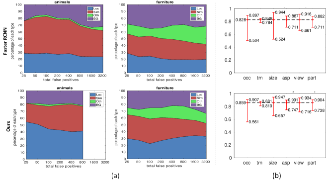
Figure 6: Analysis results between Faster RCNN (top row) and our methods (bottom row) by Hoiem et al. (2012). Left of the dashed line: distribution of top false positive types. Right of the dashed line: sensitivity to object characteristics.

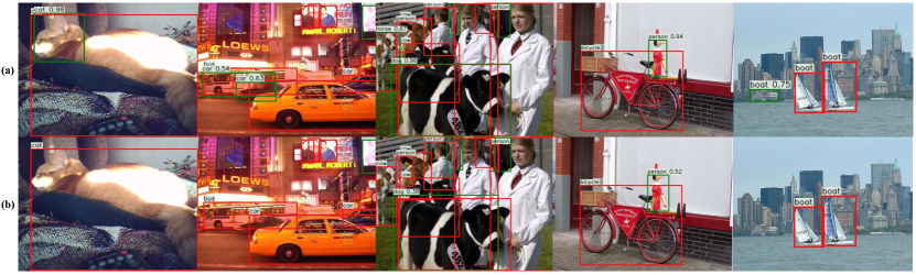
Figure 7: Comparison of hard false positives with confidence score higher than 0.3 between Faster RCNN and Our methods. Red box: ground truth object. Green box: hard false positive. Row (a), results from Faster RCNN. Row (b), results of our DCR module.

5.6.1 Error Analysis

Following Girshick et al. (2014), we also use the detection analysis tool from Hoiem et al. (2012), in order to gather more information of the error mode of Faster RCNN and DCR module. Analysis results are shown in Fig 6.

Fig 6 (a) shows the distribution of top false positive types as scores decrease. False positives are classified into four categories: (1) Loc: IOU with ground truth boxes is in the range of $[0.1,0.5)$; (2) Sim: detections have at least 0.1 IOU with objects in predefined similar classes, e.g. dog and cat are similar classes; (3) Oth: detections have at least 0.1 IOU with objects not in predefined similar classes; (4) BG: all other false positives are considered background. We observe that comparing with Faster RCNN, DCR module has much larger ratio of localization error and the number of false positives is greatly reduced on some classes, e.g. in the animal class, the number of false positives is largely reduced by 4 times and initial percentage of localization error increases from less than 30% to over 50%. This statistics are consistent with motivations to reducing classification errors by reducing number of false positives.

Fig 6 (b) compares the sensitivity of Faster RCNN and DCR to object characteristics. Hoiem et al. (2012) defines object with six characteristics: (1) occ: occlusion, where an object is occluded by another surface; (2) trn: truncation, where there is only part of an object; (3) size: the size of an object measure by the pixel area; (4) asp: aspect ratio of an object; (5) view: whether each side of an object is visible; (6) part: whether each part of an object is visible. Normalized AP is used to measure detectors performance and more details can be found in Hoiem et al. (2012). In general, the higher the normalized AP, the better the performance. The difference between max and min value measure the sensibility of a detector, the smaller the difference, the less sensible of a detector. We observe that DCR improves normalized AP and sensitivity on all types of object and improves sensitivity significantly on occlusion and size. This increase came from the adaptive field of DCR, since DCR can focus only on the object area, making it less sensible to occlusion and size of objects.

5.7 Visualization

We visualize all false positives with confidence larger than 0.3 for both Faster RCNN and our DCR module in Fig 7. We observe that the DCR module successfully suppresses all three kinds of hard false positives to some extends.

The first image shows reducing the first type of false positives (part of objects). Faster RCNN (top) classifies the head of the cat with a extremely high confidence (0.98) but it is eliminated by the DCR module.

The second to the fourth images demonstrate situations of second type of false positives (similar objects) where most of false positives are suppressed (“car” in the second image and “horse” in the third image). However, we find there still exists some limitations, e.g. the “dog” in the third image where it is supposed to be a cow and the “person” in the fourth image. Although they are not suppressed, their scores are reduced significantly (0.96 $\rightarrow$ 0.38 and 0.92 $\rightarrow$ 0.52 respectively) which will also improve the overall performance. It still remains an open questions to solve these problems. We hypothesize that by using more training data of such hard false positives (e.g. use data augmentation to generate such samples).

The last image shows example for the third type of false positives (backgrounds). A part of background near the ground truth is classified as a “boat” by the Faster RCNN and it is successfully eliminated by our DCR module.

6 Conclusion

In this paper, we analyze error modes of state-of-the-art region-based object detectors and study their potentials in accuracy improvement. We hypothesize that good object detectors should be designed following three principles: decoupled features, decoupled optimization and adaptive receptive field. Based on these principles, we propose a simple, effective and widely-applicable DCR module that achieves new state-of-the-art. Furthermore, we use experiments to support that a good detector should have decoupled features and adaptive receptive field and we observe an interesting novel trade-off between feature sharing and speed/accuracy. In the future, we will further study what architecture makes a good object detector, adaptive feature representation in multi-task learning, and efficiency improvement of our DCR module. We hope this paper could motivate the community to study new directions of improving current object detection frameworks. Specifically, (1) DCR module still has 4.3% mAP to be improved due to false positives and how to suppress these remaining false positives remains an open question. (2) how to design more efficient decoupled structure is yet another interesting research direction.

References

- Bourdev and Brandt (2005) Bourdev L, Brandt J (2005) Robust object detection via soft cascade. In: IEEE CVPR
- Cai and Vasconcelos (2018) Cai Z, Vasconcelos N (2018) Cascade r-cnn: Delving into high quality object detection. In: IEEE CVPR
- Cao et al. (2017) Cao Z, Simon T, Wei SE, Sheikh Y (2017) Realtime multi-person 2d pose estimation using part affinity fields. In: IEEE CVPR
- Chen et al. (2018) Chen LC, Zhu Y, Papandreou G, Schroff F, Adam H (2018) Encoder-decoder with atrous separable convolution for semantic image segmentation. In: ECCV
- Cheng et al. (2018) Cheng B, Wei Y, Shi H, Feris R, Xiong J, Huang T (2018) Revisiting rcnn: On awakening the classification power of faster rcnn. In: ECCV
- Cheng et al. (2019a) Cheng B, Chen LC, Wei Y, Zhu Y, Huang Z, Xiong J, Huang TS, Hwu WM, Shi H (2019a) Spgnet: Semantic prediction guidance for scene parsing. In: IEEE ICCV
- Cheng et al. (2019b) Cheng B, Collins MD, Zhu Y, Liu T, Huang TS, Adam H, Chen LC (2019b) Panoptic-deeplab. arXiv preprint arXiv:191004751
- Cheng et al. (2019c) Cheng B, Collins MD, Zhu Y, Liu T, Huang TS, Adam H, Chen LC (2019c) Panoptic-deeplab: A simple, strong, and fast baseline for bottom-up panoptic segmentation. arXiv preprint arXiv:191110194
- Cheng et al. (2019d) Cheng B, Xiao B, Wang J, Shi H, Huang TS, Zhang L (2019d) Bottom-up higher-resolution networks for multi-person pose estimation. arXiv preprint arXiv:190810357
- Dai et al. (2016) Dai J, Li Y, He K, Sun J (2016) R-fcn: Object detection via region-based fully convolutional networks. In: NIPS
- Dai et al. (2017) Dai J, Qi H, Xiong Y, Li Y, Zhang G, Hu H, Wei Y (2017) Deformable convolutional networks. In: IEEE ICCV
- Deng et al. (2009) Deng J, Dong W, Socher R, Li LJ, Li K, Fei-Fei L (2009) Imagenet: A large-scale hierarchical image database. In: IEEE CVPR
- Duan et al. (2019) Duan K, Bai S, Xie L, Qi H, Huang Q, Tian Q (2019) Centernet: Keypoint triplets for object detection. In: IEEE ICCV
- Everingham et al. (2010) Everingham M, Van Gool L, Williams CKI, Winn J, Zisserman A (2010) The pascal visual object classes (voc) challenge. IJCV
- Felzenszwalb et al. (2010) Felzenszwalb PF, Girshick RB, McAllester D, Ramanan D (2010) Object detection with discriminatively trained part-based models. IEEE TPAMI
- Freund and Schapire (1997) Freund Y, Schapire RE (1997) A decision-theoretic generalization of on-line learning and an application to boosting. Journal of computer and system sciences
- Fu et al. (2017) Fu CY, Liu W, Ranga A, Tyagi A, Berg AC (2017) Dssd: Deconvolutional single shot detector. arXiv preprint arXiv:170106659
- Girshick (2015) Girshick R (2015) Fast r-cnn. In: IEEE ICCV
- Girshick et al. (2014) Girshick R, Donahue J, Darrell T, Malik J (2014) Rich feature hierarchies for accurate object detection and semantic segmentation. In: IEEE CVPR
- Goyal et al. (2017) Goyal P, Dollár P, Girshick R, Noordhuis P, Wesolowski L, Kyrola A, Tulloch A, Jia Y, He K (2017) Accurate, large minibatch sgd: training imagenet in 1 hour. arXiv preprint arXiv:170602677
- He et al. (2014) He K, Zhang X, Ren S, Sun J (2014) Spatial pyramid pooling in deep convolutional networks for visual recognition. In: ECCV
- He et al. (2016) He K, Zhang X, Ren S, Sun J (2016) Deep residual learning for image recognition. In: IEEE CVPR
- He et al. (2017) He K, Gkioxari G, Dollár P, Girshick R (2017) Mask r-cnn. In: IEEE ICCV
- Hoiem et al. (2012) Hoiem D, Chodpathumwan Y, Dai Q (2012) Diagnosing error in object detectors. In: ECCV
- Hu et al. (2018) Hu H, Gu J, Zhang Z, Dai J, Wei Y (2018) Relation networks for object detection. In: IEEE CVPR
- Huang et al. (2019) Huang Z, Huang L, Gong Y, Huang C, Wang X (2019) Mask scoring r-cnn. In: IEEE CVPR
- Jiang et al. (2018) Jiang B, Luo R, Mao J, Xiao T, Jiang Y (2018) Acquisition of localization confidence for accurate object detection. In: ECCV
- Law and Deng (2018) Law H, Deng J (2018) Cornernet: Detecting objects as paired keypoints. In: ECCV
- Li et al. (2015) Li H, Lin Z, Shen X, Brandt J, Hua G (2015) A convolutional neural network cascade for face detection. In: IEEE CVPR
- Li et al. (2017a) Li J, Liang X, Wei Y, Xu T, Feng J, Yan S (2017a) Perceptual generative adversarial networks for small object detection. In: IEEE CVPR
- Li et al. (2017b) Li J, Wei Y, Liang X, Dong J, Xu T, Feng J, Yan S (2017b) Attentive contexts for object detection. IEEE Transactions on Multimedia
- Li et al. (2018a) Li J, Liang X, Li J, Wei Y, Xu T, Feng J, Yan S (2018a) Multistage object detection with group recursive learning. IEEE Transactions on Multimedia
- Li et al. (2018b) Li Z, Peng C, Yu G, Zhang X, Deng Y, Sun J (2018b) Detnet: Design backbone for object detection. In: ECCV
- Lin et al. (2014) Lin TY, Maire M, Belongie S, Hays J, Perona P, Ramanan D, Dollár P, Zitnick CL (2014) Microsoft coco: Common objects in context. In: ECCV
- Lin et al. (2017a) Lin TY, Dollár P, Girshick R, He K, Hariharan B, Belongie S (2017a) Feature pyramid networks for object detection. In: IEEE CVPR
- Lin et al. (2017b) Lin TY, Goyal P, Girshick R, He K, Dollar P (2017b) Focal loss for dense object detection. In: IEEE ICCV
- Liu et al. (2016) Liu W, Anguelov D, Erhan D, Szegedy C, Reed S, Fu CY, Berg AC (2016) Ssd: Single shot multibox detector. In: ECCV
- Long et al. (2015) Long J, Shelhamer E, Darrell T (2015) Fully convolutional networks for semantic segmentation. In: IEEE CVPR
- Papandreou et al. (2017) Papandreou G, Zhu T, Kanazawa N, Toshev A, Tompson J, Bregler C, Murphy K (2017) Towards accurate multi-person pose estimation in the wild. In: IEEE CVPR
- Redmon and Farhadi (2017) Redmon J, Farhadi A (2017) Yolo9000: Better, faster, stronger. In: IEEE CVPR
- Redmon et al. (2016) Redmon J, Divvala S, Girshick R, Farhadi A (2016) You only look once: Unified, real-time object detection. In: IEEE CVPR
- Ren et al. (2015) Ren S, He K, Girshick R, Sun J (2015) Faster r-cnn: Towards real-time object detection with region proposal networks. In: NIPS
- Sermanet et al. (2013) Sermanet P, Eigen D, Zhang X, Mathieu M, Fergus R, LeCun Y (2013) Overfeat: Integrated recognition, localization and detection using convolutional networks. arXiv preprint arXiv:13126229
- Shen et al. (2019) Shen Z, Shi H, Yu J, Phan H, Feris R, Cao L, Liu D, Wang X, Huang T, Savvides M (2019) Improving object detection from scratch via gated feature reuse. In: BMVC
- Singh and Davis (2018) Singh B, Davis LS (2018) An analysis of scale invariance in object detection–snip. In: IEEE CVPR
- Tian et al. (2019) Tian Z, Shen C, Chen H, He T (2019) Fcos: Fully convolutional one-stage object detection. In: IEEE ICCV
- Uijlings et al. (2013) Uijlings JR, Van De Sande KE, Gevers T, Smeulders AW (2013) Selective search for object recognition. IJCV
- Viola and Jones (2004) Viola P, Jones MJ (2004) Robust real-time face detection. IJCV
- Wei et al. (2018) Wei Y, Shen Z, Cheng B, Shi H, Xiong J, Feng J, Huang T (2018) Ts2c: Tight box mining with surrounding segmentation context for weakly supervised object detection. In: European Conference on Computer Vision
- Xie et al. (2017) Xie S, Girshick R, Dollár P, Tu Z, He K (2017) Aggregated residual transformations for deep neural networks. In: IEEE CVPR
- Xu et al. (2017) Xu H, Lv X, Wang X, Ren Z, Chellappa R (2017) Deep regionlets for object detection. ECCV
- Yang et al. (2016) Yang B, Yan J, Lei Z, Li SZ (2016) Craft objects from images. In: IEEE CVPR
- Yu et al. (2016) Yu J, Jiang Y, Wang Z, Cao Z, Huang T (2016) Unitbox: An advanced object detection network. In: Proceedings of the 2016 ACM on Multimedia Conference, ACM
- Zhou et al. (2019a) Zhou X, Wang D, Krähenbühl P (2019a) Objects as points. arXiv preprint arXiv:190407850
- Zhou et al. (2019b) Zhou X, Zhuo J, Krahenbuhl P (2019b) Bottom-up object detection by grouping extreme and center points. In: IEEE CVPR
- Zhu et al. (2019a) Zhu C, He Y, Savvides M (2019a) Feature selective anchor-free module for single-shot object detection. In: IEEE CVPR
- Zhu et al. (2019b) Zhu X, Hu H, Lin S, Dai J (2019b) Deformable convnets v2: More deformable, better results. In: IEEE CVPR