textTOvec: Deep Contextualized Neural
Autoregressive Topic Models of Language
with Distributed Compositional Prior

Abstract

We address two challenges of probabilistic topic modelling in order to better estimate the probability of a word in a given context, i.e., $P(\mbox{word}|\mbox{context})$ : (1) No language structure in context: Probabilistic topic models ignore word order by summarizing a given context as a “bag-of-word” and consequently the semantics of words in the context is lost. In this work, we incorporate language structure by combining a neural autoregressive topic model (TM) (e.g., DocNADE) with a LSTM based language model (LSTM-LM) in a single probabilistic framework. The LSTM-LM learns a vector-space representation of each word by accounting for word order in local collocation patterns, while the TM simultaneously learns a latent representation from the entire document. In addition, the LSTM-LM models complex characteristics of language (e.g., syntax and semantics), while the TM discovers the underlying thematic structure in a collection of documents. We unite two complementary paradigms of learning the meaning of word occurrences by combining a topic model and a language model in a unified probabilistic framework, named as ctx-DocNADE. (2) Limited context and/or smaller training corpus of documents: In settings with a small number of word occurrences (i.e., lack of context) in short text or data sparsity in a corpus of few documents, the application of TMs is challenging. We address this challenge by incorporating external knowledge into neural autoregressive topic models via a language modelling approach: we use word embeddings as input of a LSTM-LM with the aim to improve the word-topic mapping on a smaller and/or short-text corpus. The proposed DocNADE extension is named as ctx-DocNADEe.

We present novel neural autoregressive topic model variants coupled with neural language models and embeddings priors that consistently outperform state-of-the-art generative topic models in terms of generalization (perplexity), interpretability (topic coherence) and applicability (retrieval and classification) over 7 long-text and 8 short-text datasets from diverse domains.

1 Introduction

Probabilistic topic models, such as LDA (Blei et al., 2003), Replicated Softmax (RSM) (Salakhutdinov & Hinton, 2009) and Document Neural Autoregressive Distribution Estimator (DocNADE) variants (Larochelle & Lauly, 2012; Zheng et al., 2016; Lauly et al., 2017; Gupta et al., 2019) are often used to extract topics from text collections, and predict the probabilities of each word in a given document belonging to each topic. Subsequently, they learn latent document representations that can be used to perform natural language processing (NLP) tasks such as information retrieval (IR), document classification or summarization. However, such probabilistic topic models ignore word order and represent a given context as a bag of its words, thereby disregarding semantic information.

To motivate our first task of extending probabilistic topic models to incorporate word order and language structure, assume that we conduct topic analysis on the following two sentences:

Bear falls into market territory and Market falls into bear territory

When estimating the probability of a word in a given context (here: $P(``bear"|\mbox{context})$), traditional topic models do not account for language structure since they ignore word order within the context and are based on “bag-of-words” (BoWs) only. In this particular setting, the two sentences have the same unigram statistics, but are about different topics. On deciding which topic generated the word “bear” in the second sentence, the preceding words “market falls” make it more likely that it was generated by a topic that assigns a high probability to words related to stock market trading, where “bear territory” is a colloquial expression in the domain. In addition, the language structure (e.g., syntax and semantics) is also ignored. For instance, the word “bear” in the first sentence is a proper noun and subject while it is an object in the second. In practice, topic models also ignore functional words such as “into”, which may not be appropriate in some scenarios.

Recently, Peters et al. (2018) have shown that a deep contextualized LSTM-based language model (LSTM-LM) is able to capture different language concepts in a layer-wise fashion, e.g., the lowest layer captures language syntax and topmost layer captures semantics. However, in LSTM-LMs the probability of a word is a function of its sentence only and word occurrences are modeled in a fine granularity. Consequently, LSTM-LMs do not capture semantics at a document level. To this end, recent studies such as TDLM (Lau et al., 2017), Topic-RNN (Dieng et al., 2016) and TCNLM (Wang et al., 2018) have integrated the merits of latent topic and neural language models (LMs); however, they have focused on improving LMs with global (semantics) dependencies using latent topics.

Similarly, while bi-gram LDA based topic models (Wallach, 2006; Wang et al., 2007) and n-gram based topic learning (Lauly et al., 2017) can capture word order in short contexts, they are unable to capture long term dependencies and language concepts. In contrast, DocNADE variants (Larochelle & Lauly, 2012; Gupta et al., 2019) learns word occurrences across documents i.e., coarse granularity (in the sense that the topic assigned to a given word occurrence equally depends on all the other words appearing in the same document); however since it is based on the BoW assumption all language structure is ignored. In language modeling, Mikolov et al. (2010) have shown that recurrent neural networks result in a significant reduction of perplexity over standard n-gram models.

Contribution 1: We introduce language structure into neural autoregressive topic models via a LSTM-LM, thereby accounting for word ordering (or semantic regularities), language concepts and long-range dependencies. This allows for the accurate prediction of words, where the probability of each word is a function of global and local (semantics) contexts, modeled via DocNADE and LSTM-LM, respectively. The proposed neural topic model is named as contextualized-Document Neural Autoregressive Distribution Estimator (ctx-DocNADE) and offers learning complementary semantics by combining joint word and latent topic learning in a unified neural autoregressive framework. For instance, Figure 1 (left and middle) shows the complementary topic and word semantics, based on TM and LM representations of the term “fall”. Observe that the topic captures the usage of “fall” in the context of stock market trading, attributed to the global (semantic) view.

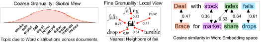
Figure 1: (left): A topic-word distribution due to global exposure, obtained from the matrix ${\bf W}$ as row-vector. (middle): Nearest neighbors in semantics space, represented by ${\bf W}$ in its column vectors. (right): BoW and cosine similarity illustration in distributed embedding space.

While this is a powerful approach for incorporating language structure and word order in particular for long texts and corpora with many documents, learning from contextual information remains challenging in settings with short texts and few documents, since (1) limited word co-occurrences or little context (2) significant word non-overlap in such short texts and (3) small training corpus of documents lead to little evidence for learning word co-occurrences. However, distributional word representations (i.e. word embeddings) (Pennington et al., 2014) have shown to capture both the semantic and syntactic relatedness in words and demonstrated impressive performance in NLP tasks.

For example, assume that we conduct topic analysis over the two short text fragments: Deal with stock index falls and Brace for market share drops. Traditional topic models with “BoW” assumption will not be able to infer relatedness between word pairs such as (falls, drops) due to the lack of word-overlap and small context in the two phrases. However, in the distributed embedding space, the word pairs are semantically related as shown in Figure 1 (left).

Related work such as Sahami & Heilman (2006) employed web search results to improve the information in short texts and Petterson et al. (2010) introduced word similarity via thesauri and dictionaries into LDA. Das et al. (2015) and Nguyen et al. (2015) integrated word embeddings into LDA and Dirichlet Multinomial Mixture (DMM) (Nigam et al., 2000) models. Recently, Gupta et al. (2019) extends DocNADE by introducing pre-trained word embeddings in topic learning. However, they ignore the underlying language structure, e.g., word ordering, syntax, etc. In addition, DocNADE and its extensions outperform LDA and RSM topic models in terms of perplexity and IR.

Contribution 2: We incorporate distributed compositional priors in DocNADE: we use pre-trained word embeddings via LSTM-LM to supplement the multinomial topic model (i.e., DocNADE) in learning latent topic and textual representations on a smaller corpus and/or short texts. Knowing similarities in a distributed space and integrating this complementary information via a LSTM-LM, a topic representation is much more likely and coherent.

Taken together, we combine the advantages of complementary learning and external knowledge, and couple topic- and language models with pre-trained word embeddings to model short and long text documents in a unified neural autoregressive framework, named as ctx-DocNADEe. Our approach learns better textual representations, which we quantify via generalizability (e.g., perplexity), interpretability (e.g., topic extraction and coherence) and applicability (e.g., IR and classification).

To illustrate our two contributions, we apply our modeling approaches to 7 long-text and 8 short-text datasets from diverse domains and demonstrate that our approach consistently outperforms state-of-the-art generative topic models. Our learned representations, result in a gain of: (1) $4.6$% (.790 vs .755) in topic coherence, (2) $6.5$% (.615 vs .577) in precision at retrieval fraction 0.02, and (3) $4.4$% (.662 vs .634) in $F1$ for text classification, averaged over 6 long-text and 8 short-text datasets.

When applied to short-text and long-text documents, our proposed modeling approaches generate contextualized topic vectors, which we name textTOvec. The code is available at https://github.com/pgcool/textTOvec.

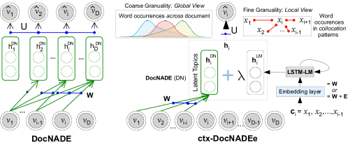
Figure 2: (left): DocNADE for the document ${\bf v}$. (right): ctx-DocNADEe for the observable corresponding to $v_{i}\in{\bf v}$. Blue colored lines signify the connections that share parameters. The observations (double circle) for each word $v_{i}$ are multinomial, where $v_{i}$ is the index in the vocabulary of the $i$th word of the document. ${\bf h}_{i}^{DN}$ and ${\bf h}_{i}^{LM}$ are hidden vectors from DocNADE and LSTM models, respectively for the target word $v_{i}$. Connections between each input $v_{i}$ and hidden units ${\bf h}_{i}^{DN}$ are shared. The symbol $\hat{v}_{i}$ represents the autoregressive conditionals $p(v_{i}|{\bf v}_{<i})$, computed using ${\bf h}_{i}$ which is a weighted sum of ${\bf h}_{i}^{DN}$ and ${\bf h}_{i}^{LM}$ in ctx-DocNADEe.

2 Neural Autoregressive Topic Models

Generative models are based on estimating the probability distribution of multidimensional data, implicitly requiring modeling complex dependencies. Restricted Boltzmann Machine (RBM) (Hinton et al., 2006) and its variants (Larochelle & Bengio, 2008) are probabilistic undirected models of binary data. RSM (Salakhutdinov & Hinton, 2009) and its variants (Gupta et al., 2018) are generalization of the RBM, that are used to model word counts. However, estimating the complex probability distribution of the underlying high-dimensional observations is intractable. To address this challenge, NADE (Larochelle & Murray, 2011) decomposes the joint distribution of binary observations into autoregressive conditional distributions, each modeled using a feed-forward network. Unlike for RBM/RSM, this leads to tractable gradients of the data negative log-likelihood.

2.1 Document Neural Autoregressive Topic Model (DocNADE)

An extension of NADE and RSM, DocNADE (Larochelle & Lauly, 2012) models collections of documents as orderless bags of words (BoW approach), thereby disregarding any language structure. In other words, it is trained to learn word representations reflecting the underlying topics of the documents only, ignoring syntactical and semantic features as those encoded in word embeddings (Bengio et al., 2003; Mikolov et al., 2013; Pennington et al., 2014; Peters et al., 2018).

DocNADE (Lauly et al., 2017) represents a document by transforming its BoWs into a sequence ${\bf v}=[v_{1},...,v_{D}]$ of size $D$, where each element $v_{i}\in\{1,2,...,K\}$ corresponds to a multinomial observation (representing a word from a vocabulary of size $K$). Thus, $v_{i}$ is the index in the vocabulary of the $i$th word of the document v. DocNADE models the joint distribution $p({\bf v})$ of all words $v_{i}$ by decomposing it as $p({\bf v})=\prod_{i=1}^{D}p(v_{i}|{\bf v}_{<i})$, where each autoregressive conditional $p(v_{i}|{\bf v}_{<i})$ for the word observation $v_{i}$ is computed using the preceding observations ${\bf v}_{<i}\in\{v_{1},...,v_{i-1}\}$ in a feed-forward neural network for $i\in\{1,...D\}$,

$${\bf h}_{i}^{DN}({\bf v}_{<i})=g({\bf e}+\sum_{k<i}{\bf W}_{:,v_{k}})\ \ \mbox{and}\ \ p(v_{i}=w|{\bf v}_{<i})=\frac{\exp(b_{w}+{\bf U}_{w,:}{\bf h}_{i}^{DN}({\bf v}_{<i}))}{\sum_{w^{\prime}}\exp(b_{w^{\prime}}+{\bf U}_{w^{\prime},:}{\bf h}_{i}^{DN}({\bf v}_{<i}))}$$ (1)

where $g(\cdot)$ is an activation function, ${\bf U}\in\mathbb{R}^{K\times H}$ is a weight matrix connecting hidden to output, ${\bf e}\in\mathbb{R}^{H}$ and ${\bf b}\in\mathbb{R}^{K}$ are bias vectors, ${\bf W}\in\mathbb{R}^{H\times K}$ is a word representation matrix in which a column ${\bf W}_{:,v_{i}}$ is a vector representation of the word $v_{i}$ in the vocabulary, and $H$ is the number of hidden units (topics). The log-likelihood of any document ${\bf v}$ of any arbitrary length is given by: $\mathcal{L}^{DN}({\bf v})=\sum_{i=1}^{D}\log p(v_{i}|{\bf v}_{<i})$. Note that the past word observations ${\bf v}_{<i}$ are orderless due to BoWs, and may not correspond to the words preceding the $i$th word in the document itself.

Algorithm 1 Computation of $\log p({\bf v})$

1:Input: A training document v

2:Input: Word embedding matrix E

3:Output: $\log p({\bf v})$

4:${\bf a}\leftarrow{\bf e}$

5:$q({\bf v})=1$

6:for $i$ from $1$ to $D$ do

7:     compute ${\bf h}_{i}$ and $p(v_{i}|{\bf v}_{<i})$

8:     $q({\bf v})\leftarrow q({\bf v})p(v_{i}|{\bf v}_{<i})$

9:     ${\bf a}\leftarrow{\bf a}+{\bf W}_{:,v_{i}}$

10:$\log p({\bf v})\leftarrow\log q({\bf v})$

model	${\bf h}_{i}$	$p(v_{i}|{\bf v}_{<i})$
DocNADE	${\bf h}_{i}^{DN}\leftarrow g({\bf a})$	equation 1
	${\bf h}_{i}\leftarrow{\bf h}_{i}^{DN}$
ctx-DocNADE	${\bf h}_{i}^{LM}\leftarrow\mbox{LSTM}({\bf c}_{i},\mbox{embedding}={\bf W})$	equation 2
	${\bf h}_{i}\leftarrow{\bf h}_{i}^{DN}+\lambda\ {\bf h}_{i}^{LM}$
ctx-DocNADEe	${\bf h}_{i}^{LM}\leftarrow\mbox{LSTM}({\bf c}_{i},\mbox{embedding}={\bf W}+{\bf E})$	equation 2
	${\bf h}_{i}\leftarrow{\bf h}_{i}^{DN}+\lambda\ {\bf h}_{i}^{LM}$

Table 1: Computation of ${\bf h}_{i}$ and $p(v_{i}|{\bf v}_{<i})$ in DocNADE, ctx-DocNADE and ctx-DocNADEe models, correspondingly used in estimating $\log p({\bf v})$ (Algorithm 1).

2.2 Deep Contextualized DocNADE with Distributional Semantics

We propose two extensions of the DocNADE model: (1) ctx-DocNADE: introducing language structure via LSTM-LM and (2) ctx-DocNADEe: incorporating external knowledge via pre-trained word embeddings ${\bf E}$, to model short and long texts. The unified network(s) account for the ordering of words, syntactical and semantic structures in a language, long and short term dependencies, as well as external knowledge, thereby circumventing the major drawbacks of BoW-based representations.

Similar to DocNADE, ctx-DocNADE models each document $\bf v$ as a sequence of multinomial observations. Let $[x_{1},x_{2},...,x_{N}]$ be a sequence of N words in a given document, where $x_{i}$ is represented by an embedding vector of dimension, $dim$. Further, for each element $v_{i}\in{\bf v}$, let ${\bf c}_{i}=[x_{1},x_{2},...,x_{i-1}]$ be the context (preceding words) of $i$th word in the document. Unlike in DocNADE, the conditional probability of the word $v_{i}$ in ctx-DocNADE (or ctx-DocNADEe) is a function of two hidden vectors: ${\bf h}_{i}^{DN}({\bf v}_{<i})$ and ${\bf h}_{i}^{LM}({\bf c}_{i})$, stemming from the DocNADE-based and LSTM-based components of ctx-DocNADE, respectively:

$${\bf h}_{i}({\bf v}_{<i})={\bf h}_{i}^{DN}({\bf v}_{<i})+\lambda\ \ {\bf h}_{i}^{LM}({\bf c}_{i})\ \mbox{and}\ p(v_{i}=w|{\bf v}_{<i})=\frac{\exp(b_{w}+{\bf U}_{w,:}{\bf h}_{i}({\bf v}_{<i}))}{\sum_{w^{\prime}}\exp(b_{w^{\prime}}+{\bf U}_{w^{\prime},:}{\bf h}_{i}({\bf v}_{<i}))}$$ (2)

where ${\bf h}_{i}^{DN}({\bf v}_{<i})$ is computed as in DocNADE (equation 1) and $\lambda$ is the mixture weight of the LM component, which can be optimized during training (e.g., based on the validation set). The second term ${\bf h}_{i}^{LM}$ is a context-dependent representation and output of an LSTM layer at position $i-1$ over input sequence ${\bf c}_{i}$, trained to predict the next word $v_{i}$. The LSTM offers history for the $i$th word via modeling temporal dependencies in the input sequence, ${\bf c}_{i}$. The conditional distribution for each word $v_{i}$ is estimated by equation 2, where the unified network of DocNADE and LM combines global and context-dependent representations. Our model is jointly optimized to maximize the pseudo log likelihood, $\log p({\bf v})\approx\sum_{i=1}^{D}\log p(v_{i}|{\bf v}_{<i})$ with stochastic gradient descent. See Larochelle & Lauly (2012) for more details on training from bag of word counts.

In the weight matrix $\bf W$ of DocNADE (Larochelle & Lauly, 2012), each row vector ${\bf W}_{j,:}$ encodes topic information for the $j$th hidden topic feature and each column vector ${\bf W}_{:,v_{i}}$ is a vector for the word $v_{i}$. To obtain complementary semantics, we exploit this property and expose $\bf W$ to both global and local influences by sharing $\bf W$ in the DocNADE and LSTM-LM componenents. Thus, the embedding layer of LSTM-LM component represents the column vectors.

ctx-DocNADE, in this realization of the unified network the embedding layer in the LSTM component is randomly initialized. This extends DocNADE by accounting for the ordering of words and language concepts via context-dependent representations for each word in the document.

ctx-DocNADEe, the second version extends ctx-DocNADE with distributional priors, where the embedding layer in the LSTM component is initialized by the sum of a pre-trained embedding matrix ${\bf E}$ and the weight matrix ${\bf W}$. Note that ${\bf W}$ is a model parameter; however ${\bf E}$ is a static prior.

Algorithm 1 and Table 1 show the $\log p({\bf v})$ for a document ${\bf v}$ in three different settings: DocNADE, ctx-DocNADE and ctx-DocNADEe. In the DocNADE component, since the weights in the matrix ${\bf W}$ are tied, the linear activation ${\bf a}$ can be re-used in every hidden layer and computational complexity reduces to $O(HD)$, where H is the size of each hidden layer. In every epoch, we run an LSTM over the sequence of words in the document and extract hidden vectors $h_{i}^{LM}$, corresponding to ${\bf c}_{i}$ for every target word $v_{i}$. Therefore, the computational complexity in ctx-DocNADE or ctx-DocNADEe is $O(HD+\mathfrak{N})$, where $\mathfrak{N}$ is the total number of edges in the LSTM network (Hochreiter & Schmidhuber, 1997; Sak et al., 2014). The trained models can be used to extract a textTOvec representation, i.e., ${\bf h}({\bf v}^{*})={\bf h}^{DN}({\bf v}^{*})+\lambda\ {\bf h}^{LM}({\bf c}^{*}_{N+1})$ for the text ${\bf v}^{*}$ of length ${\bf D}^{*}$, where ${\bf h}^{DN}({\bf v}^{*})=g({\bf e}+\sum_{k\leq{\bf D}^{*}}{\bf W}_{:,v_{k}})$ and ${\bf h}^{LM}({\bf c}^{*}_{N+1})=\mbox{LSTM}({\bf c}^{*}_{{N+1}},\mbox{embedding}={\bf W}\mbox{ or }({\bf W}+{\bf E}))$.

short-text									long-text
Data	Train	Val	Test	$|$RV$|$	$|$FV$|$	L	C	Domain	Data	Train	Val	Test	$|$RV$|$	$|$FV$|$	L	C	Domain
20NSshort	1.3k	0.1k	0.5k	1.4k	1.4k	13.5	20	News	20NSsmall	0.4k	0.2k	0.2k	2k	4555	187.5	20	News
TREC6	5.5k	0.5k	0.5k	2k	2295	9.8	6	Q&A	Reuters8	5.0k	0.5k	2.2k	2k	7654	102	8	News
R21578title†	7.3k	0.5k	3.0k	2k	2721	7.3	90	News	20NS	7.9k	1.6k	5.2k	2k	33770	107.5	20	News
Subjectivity	8.0k	.05k	2.0k	2k	7965	23.1	2	Senti	R21578†	7.3k	0.5k	3.0k	2k	11396	128	90	News
Polarity	8.5k	.05k	2.1k	2k	7157	21.0	2	Senti	BNC	15.0k	1.0k	1.0k	9.7k	41370	1189	-	News
TMNtitle	22.8k	2.0k	7.8k	2k	6240	4.9	7	News	SiROBs†	27.0k	1.0k	10.5k	3k	9113	39	22	Indus
TMN	22.8k	2.0k	7.8k	2k	12867	19	7	News	AGNews	118k	2.0k	7.6k	5k	34071	38	4	News
AGnewstitle	118k	2.0k	7.6k	5k	17125	6.8	4	News

Table 2: Data statistics: Short/long texts and/or small/large corpora from diverse domains. Symbols- Avg: average, $L$: avg text length (#words), $|RV|$ and $|FV|$: size of reduced (RV) and full vocabulary (FV), $C$: number of classes, Senti: Sentiment, Indus: Industrial, ‘k’:thousand and $\dagger$: multi-label. For short-text, $L$$<$$25$.

ctx-DeepDNEe: DocNADE and LSTM can be extended to a deep, multiple hidden layer architecture by adding new hidden layers as in a regular deep feed-forward neural network, allowing for improved performance. In the deep version, the first hidden layer is computed in an analogous fashion to DocNADE variants (equation 1 or 2). Subsequent hidden layers are computed as:

$${\bf h}_{i,d}^{DN}({\bf v}_{<i})=g({\bf e}_{d}+{\bf W}_{i,d}\cdot{\bf h}_{i,d-1}({\bf v}_{<i}))\ \ \mbox{or}\ \ {\bf h}_{i,d}^{LM}({\bf c}_{i})=deepLSTM({\bf c}_{i},\mbox{depth}=d)$$

for $d=2,...n$, where n is the total number of hidden layers (i.e., depth) in the deep feed-forward and LSTM networks. For $d$=$1$, the hidden vectors ${\bf h}_{i,1}^{DN}$ and ${\bf h}_{i,1}^{LM}$ correspond to equations 1 and 2. The conditional $p(v_{i}=w|{\bf v}_{<i})$ is computed using the last layer $n$, i.e., ${\bf h}_{i,n}={\bf h}_{i,n}^{DN}+\lambda\ {\bf h}_{i,n}^{LM}$.

Model	20NSshort		TREC6		R21578title		Subjectivity		Polarity		TMNtitle		TMN		AGnewstitle		Avg
	IR	$F1$	IR	$F1$	IR	$F1$	IR	$F1$	IR	$F1$	IR	$F1$	IR	$F1$	IR	$F1$	IR	$F1$
glove(RV)	.236	.493	.480	.798	.587	.356	.754	.882	.543	.715	.513	.693	.638	.736	.588	814	.542	.685
glove(FV)	.236	.488	.480	.785	.595	.356	.775	.901	.553	.728	.545	.736	.643	.813	.612	.830	.554	.704
doc2vec	.090	.413	.260	.400	.518	.176	.571	.763	.510	.624	.190	.582	.220	.720	.265	.600	.328	.534
Gauss-LDA	.080	.118	.325	.202	.367	.012	.558	.676	.505	.511	.408	.472	.713	.692	.516	.752	.434	.429
glove-DMM	.183	.213	.370	.454	.273	.011	.738	.834	.515	.585	.445	.590	.551	.666	.540	.652	.451	.500
glove-LDA	.160	.320	.300	.600	.387	.052	.610	.805	.517	.607	.260	.412	.428	.627	.547	.687	.401	.513
TDLM	.219	.308	.521	.671	.563	.174	.839	.885	.520	.599	.535	.657	.672	.767	.534	.722	.550	.586
DocNADE(RV)	.290	.440	.550	.804	.657	.313	.820	.889	.560	.699	.524	.664	.652	.759	.656	.819	.588	.673
DocNADE(FV)	.290	.440	.546	.791	.654	.302	.848	.907	.576	.724	.525	.688	.687	.796	.678	.821	.600	.683
DeepDNE	.100	.080	.479	.629	.630	.221	.865	.909	.503	.531	.536	.661	.671	.783	.682	.825	.558	.560
ctx-DocNADE	.296	.440	.595	.817	.641	.300	.874	.910	.591	.725	.560	.687	.692	.793	.691	.826	.617	.688
ctx-DocNADEe	.306	.490	.599	.824	.656	.308	.874	.917	.605	.740	.595	.726	.698	.806	.703	.828	.630	.705
ctx-DeepDNEe	.278	.416	.606	.804	.647	.244	.878	.920	.591	.723	.576	.694	.687	.796	.689	.826	.620	.688

Table 3: State-of-the-art comparison: IR (i.e, IR-precision at 0.02 fraction) and classification $F1$ for short texts, where $Avg$: average over the row values, the bold and underline: the maximum for IR and F1, respectively.

3 Evaluation

We apply our modeling approaches (in improving topic models, i.e, DocNADE using language concepts from LSTM-LM) to 8 short-text and 7 long-text datasets of varying size with single/multi-class labeled documents from public as well as industrial corpora. We present four quantitative measures in evaluating topic models: generalization (perplexity), topic coherence, text retrieval and categorization. See the appendices for the data description and example texts. Table 2 shows the data statistics, where 20NS and R21578 signify 20NewsGroups and Reuters21578, respectively.

Baselines: While, we evaluate our multi-fold contributions on four tasks: generalization (perplexity), topic coherence, text retrieval and categorization, we compare performance of our proposed models ctx-DocNADE and ctx-DocNADEe with related baselines based on: (1) word representation: glove (Pennington et al., 2014), where a document is represented by summing the embedding vectors of it’s words, (2) document representation: doc2vec (Le & Mikolov, 2014), (3) LDA based BoW TMs: ProdLDA (Srivastava & Sutton, 2017) and SCHOLAR (Card et al., 2017) (4) neural BoW TMs: DocNADE and NTM (Cao et al., 2015) and , (5) TMs, including pre-trained word embeddings: Gauss-LDA (GaussianLDA) (Das et al., 2015), and glove-DMM, glove-LDA (Nguyen et al., 2015). (6) jointly trained topic and language models: TDLM (Lau et al., 2017), Topic-RNN (Dieng et al., 2016) and TCNLM (Wang et al., 2018).

Model	20NSsmall		Reuters8		20NS		R21578		SiROBs		AGnews		Avg
	IR	$F1$	IR	$F1$	IR	$F1$	IR	$F1$	IR	$F1$	IR	$F1$	IR	$F1$
glove(RV)	.214	.442	.845	.830	.200	.608	.644	.316	.273	.202	.725	.870	.483	.544
glove(FV)	.238	.494	.837	.880	.253	.632	.659	.340	.285	.217	.737	.890	.501	.575
doc2vec	.200	.450	.586	.852	.216	.691	.524	.215	.282	.226	.387	.713	.365	.524
Gauss-LDA	.090	.080	.712	.557	.142	.340	.539	.114	.232	.070	.456	.818	.361	.329
glove-DMM	.060	.134	.623	.453	.092	.187	.501	.023	.226	.050	-	-	-	-
DocNADE(RV)	.270	.530	.884	.890	.366	.644	.723	.336	.374	.298	.787	.882	.567	.596
DocNADE(FV)	.299	.509	.879	.907	.427	.727	.715	.340	.382	.308	.794	.888	.582	.613
ctx-DocNADE	.313	.526	.880	.898	.472	.732	.714	.315	.386	.309	.791	.890	.592	.611
ctx-DocNADEe	.327	.524	.883	.900	.486	.745	.721	.332	.390	.311	.796	.894	.601	.618

Table 4: IR-precision at fraction 0.02 and classification $F1$ for long texts

	Model	PPL		Model	PPL
Subjectivity	DocNADE	980	AGnewstitle	DocNADE	846
	ctx-DocNADE	968		ctx-DocNADE	822
	ctx-DocNADEe	966		ctx-DocNADEe	820
Reuters8	DocNADE	283	20NS	DocNADE	1375
	ctx-DocNADE	276		ctx-DocNADE	1358
	ctx-DocNADEe	272		ctx-DocNADEe	1361
TMNtitle	DocNADE	1437	20NSshort	DocNADE	646
	ctx-DocNADE	1430		ctx-DocNADE	656
	ctx-DocNADEe	1427		ctx-DocNADEe	648

Table 5: Generalization: PPL

Experimental Setup: DocNADE is often trained on a reduced vocabulary (RV) after pre-processing (e.g., ignoring functional words, etc.); however, we also investigate training it on full text/vocabulary (FV) (Table 2) and compute document representations to perform different evaluation tasks. The FV setting preserves the language structure, required by LSTM-LM, and allows a fair comparison of DocNADE+FV and ctx-DocNADE variants. We use the glove embedding of 200 dimensions. All the baselines and proposed models (ctx-DocNADE, ctx-DocNADEe and ctx-DeepDNEe) were run in the FV setting over 200 topics to quantify the quality of the learned representations. To better initialize the complementary learning in ctx-DocNADEs, we perform a pre-training for 10 epochs with $\lambda$ set to $0$. See the appendices for the experimental setup and hyperparameters for the following tasks, including the ablation over $\lambda$ on validation set.

We run TDLM (Lau et al., 2017) for all the short-text datasets to evaluate the quality of representations learned in the spare data setting. For a fair comparison, we set 200 topics and hidden size, and initialize with the same pre-trained word embeddings (i.e., glove) as used in the ctx-DocNADEe.

Data	glove-DMM		glove-LDA		DocNADE		ctx-DNE		ctx-DNEe		Data	glove-DMM		DocNADE		ctx-DNE		ctx-DNEe
	W10	W20	W10	W20	W10	W20	W10	W20	W10	W20		W10	W20	W10	W20	W10	W20	W10	W20
20NSshort	.512	.575	.616	.767	.669	.779	.682	.794	.696	.801	Subjectivity	.538	.433	.613	.749	.629	.767	.634	.771
TREC6	.410	.475	.551	.736	.699	.818	.714	.810	.713	.809	AGnewstitle	.584	.678	.731	.757	.739	.858	.746	.865
R21578title	.364	.458	.478	.677	.701	.812	.713	.802	.723	.834	20NSsmall	.578	.548	.508	.628	.546	.667	.565	.692
Polarity	.637	.363	.375	.468	.610	.742	.611	.756	.650	.779	Reuters8	.372	.302	.583	.710	.584	.710	.592	.714
TMNtitle	.633	.778	.651	.798	.712	.822	.716	.831	.735	.845	20NS	.458	.374	.606	.729	.615	.746	.631	.759
TMN	.705	.444	.550	.683	.642	.762	.639	.759	.709	.825	Avg (all)	.527	.452	.643	.755	.654	.772	.672	.790

Table 6: Average coherence for short and long texts over 200 topics in FV setting, where DocNADE $\leftrightarrow$ DNE

3.1 Generalization: Perplexity (PPL)

To evaluate the generative performance of the topic models, we estimate the log-probabilities for the test documents and compute the average held-out perplexity ($PPL$) per word as, $PPL=\exp\big{(}-\frac{1}{z}\sum_{t=1}^{z}\frac{1}{|{\bf v}^{t}|}\log p({\bf v}^{t})\big{)}$, where $z$ and $|{\bf v}^{t}|$ are the total number of documents and words in a document ${\bf v}^{t}$. For DocNADE, the log-probability $\log p({\bf v}^{t})\big{)}$ is computed using $\mathcal{L}^{DN}({\bf v})$; however, we ignore the mixture coefficient, i.e., $\lambda$=0 (equation 2) to compute the exact log-likelihood in ctx-DocNADE versions. The optimal $\lambda$ is determined based on the validation set. Table 5 quantitatively shows the PPL scores, where the complementary learning with $\lambda=0.01$ (optimal) in ctx-DocNADE achieves lower perplexity than the baseline DocNADE for both short and long texts, e.g., ($822$ vs $846$) and ($1358$ vs $1375$) on AGnewstitle and 20NS datasets, respectively in the FV setting.

3.2 Interpretability: Topic Coherence

We compute topic coherence (Chang et al., 2009; Newman et al., 2009; Gupta et al., 2018) to assess the meaningfulness of the underlying topics captured. We choose the coherence measure proposed by Röder et al. (2015) , which identifies context features for each topic word using a sliding window over the reference corpus. Higher scores imply more coherent topics.

We use the gensim module (radimrehurek.com/gensim/models/coherencemodel.html, coherence type = $c\_v$) to estimate coherence for each of the 200 topics (top 10 and 20 words). Table 6 shows average coherence over 200 topics, where the higher scores in ctx-DocNADE compared to DocNADE ($.772$ vs $.755$) suggest that the contextual information and language structure help in generating more coherent topics. The introduction of embeddings in ctx-DocNADEe boosts the topic coherence, leading to a gain of $4.6$% (.790 vs .755) on average over 11 datasets. Note that the proposed models also outperform the baselines methods glove-DMM and glove-LDA. Qualitatively, Table 8 illustrates an example topic from the 20NSshort text dataset for DocNADE, ctx-DocNADE and ctx-DocNADEe, where the inclusion of embeddings results in a more coherent topic.

Model	Coherence (NPMI)
	50	100	150
(sliding window=20)
LDA#	.106	.119	.119
NTM#	.081	.070	.072
TDLM(s)#	.102	.106	.100
TDLM(l)#	.095	.101	.104
Topic-RNN(s)#	.102	.108	.102
Topic-RNN(l)#	.100	.105	.097
TCNLM(s)#	.114	.111	.107
TCNLM(l)#	.101	.104	.102
DocNADE	.097	.095	.097
ctx-DocNADE*($\lambda$=0.2)	.102	.103	.102
ctx-DocNADE*($\lambda$=0.8)	.106	.105	.104
ctx-DocNADEe*($\lambda$=0.2)	.098	.101	-
ctx-DocNADEe*($\lambda$=0.8)	.105	.104	-
(sliding window=110)
DocNADE	.133	.131	.132
ctx-DocNADE*($\lambda$=0.2)	.134	.141	.138
ctx-DocNADE*($\lambda$=0.8)	.139	.142	.140
ctx-DocNADEe*($\lambda$=0.2)	.133	.139	-
ctx-DocNADEe*($\lambda$=0.8)	.135	.141	-

Topic	Model	Topic-words (ranked by their probabilities in topic)
	TCNLM#	pollution, emissions, nuclear, waste, environmental
environment	ctx-DocNADE*	ozone, pollution, emissions, warming, waste
	ctx-DocNADEe*	pollution, emissions, dioxide, warming, environmental
	TCNLM#	elections, economic, minister, political, democratic
politics	ctx-DocNADE*	elections, democracy, votes, democratic, communist
	ctx-DocNADEe*	democrat, candidate, voters, democrats, poll
	TCNLM#	album, band, guitar, music, film
art	ctx-DocNADE*	guitar, album, band, bass, tone
	ctx-DocNADEe*	guitar, album, pop, guitars, song
	TCNLM#	bedrooms, hotel, garden, situated, rooms
facilities	ctx-DocNADE*	bedrooms, queen, hotel, situated, furnished
	ctx-DocNADEe*	hotel, bedrooms, golf, resorts, relax
	TCNLM#	corp, turnover, unix, net, profits
business	ctx-DocNADE*	shares, dividend, shareholders, stock, profits
	ctx-DocNADEe*	profits, growing, net, earnings, turnover
	TCNLM#	eye, looked, hair, lips, stared
expression	ctx-DocNADE*	nodded, shook, looked, smiled, stared
	ctx-DocNADEe*	charming, smiled, nodded, dressed, eyes
	TCNLM#	courses, training, students, medau, education
education	ctx-DocNADE*	teachers, curriculum, workshops, learning, medau
	ctx-DocNADEe*	medau, pupils, teachers, schools, curriculum

Table 7: (Left): Topic coherence (NMPI) scores of different models for 50, 100 and 150 topics on BNC dataset. The sliding window is one of the hyper-parameters for computing topic coherence (Röder et al., 2015; Wang et al., 2018). A sliding window of 20 is used in TCNLM; in addition we also present results for a window of size 110. $\lambda$ is the mixture weight of the LM component in the topic modeling process, and (s) and (l) indicate small and large model, respectively. The symbol ’-’ indicates no result, since word embeddings of 150 dimensions are not available from glove vectors. (Right): The top 5 words of seven learnt topics from our models and TCNLM. The asterisk (*) indicates our proposed models and (#) taken from TCNLM (Wang et al., 2018).

Additional Baslines: We further compare our proposed models to other approaches that combining topic and language models, such as TDLM (Lau et al., 2017), Topic-RNN (Dieng et al., 2016) and TCNLM (Wang et al., 2018). However, the related studies focus on improving language models using topic models: in contrast, the focus of our work is on improving topic models for textual representations (short-text or long-text documents) by incorporating language concepts (e.g., word ordering, syntax, semantics, etc.) and external knowledge (e.g., word embeddings) via neural language models, as discussed in section 1.

To this end, we follow the experimental setup of the most recent work, TCNLM and quantitatively compare the performance of our models (i.e., ctx-DocNADE and ctx-DocNADEe) in terms of topic coherence (NPMI) on BNC dataset. Table 7 (left) shows NPMI scores of different models, where the results suggest that our contribution (i.e., ctx-DocNADE) of introducing language concepts into BoW topic model (i.e., DocNADE) improves topic coherence. The better performance for high values of $\lambda$ illustrates the relevance of the LM component for topic coherence (DocNADE corresponds to $\lambda$=0). Similarly, the inclusion of word embeddings (i.e., ctx-DocNADEe) results in more coherent topics than the baseline DocNADE. Importantly, while ctx-DocNADEe is motivated by sparse data settings, the BNC dataset is neither a collection of short-text nor a corpus of few documents. Consequently, ctx-DocNADEe does not show improvements in topic coherence over ctx-DocNADE.

In Table 7 (right), we further qualitatively show the top 5 words of seven topics (topic name summarized by Wang et al. (2018)) from TCNML and our models. Observe that ctx-DocNADE captures a topic expression that is a collection of only verbs in the past participle. Since the BNC dataset is unlabeled, we are here restricted to comparing model performance in terms of topic coherence only.

(a) IR: 20NSshort

(b) IR: Subjectivity

(c) IR: Polarity

(d) IR: TMNtitle

(e) IR: AGnewstitle

(f) IR: 20NS

Figure 3: Retrieval performance (IR-precision) on 6 datasets at different fractions

3.3 Applicability: Text Retrieval and Categorization

Text Retrieval: We perform a document retrieval task using the short-text and long-text documents with label information. We follow the experimental setup similar to Lauly et al. (2017), where all test documents are treated as queries to retrieve a fraction of the closest documents in the original training set using cosine similarity measure between their textTOvec representations (section 2.2). To compute retrieval precision for each fraction (e.g., $0.0001$, $0.005$, $0.01$, $0.02$, $0.05$, etc.), we average the number of retrieved training documents with the same label as the query. For multi-label datasets, we average the precision scores over multiple labels for each query. Since, Salakhutdinov & Hinton (2009) and Lauly et al. (2017) have shown that RSM and DocNADE strictly outperform LDA on this task, we solely compare DocNADE with our proposed extensions.

Table 3 and 4 show the retrieval precision scores for the short-text and long-text datasets, respectively at retrieval fraction $0.02$. Observe that the introduction of both pre-trained embeddings and language/contextual information leads to improved performance on the IR task noticeably for short texts. We also investigate topic modeling without pre-processing and filtering certain words, i.e. the FV setting and find that the DocNADE(FV) or glove(FV) improves IR precision over the baseline RV setting. Therefore, we opt for the FV in the proposed extensions. On an average over the 8 short-text and 6 long-text datasets, ctx-DocNADEe reports a gain of $7.1$% ($.630$ vs $.588$) (Table 3) $6.0$% ($.601$ vs $.567$) (Table 4), respectively in precision compared to DocNADE(RV). To further compare with TDLM, our proposed models (ctx-DocNADE and ctx-DocNADEe) outperform it by a notable margin for all the short-text datasets, i.e., a gain of 14.5% (.630 vs .550: ctx-DocNADEe vs TDLM) in IR-precision. In addition, the deep variant ($d$=3) with embeddings, i.e., ctx-DeepDNEe shows competitive performance on TREC6 and Subjectivity datasets.

Figures (3(a), 3(b), 3(c), 3(d), 3(e) and 3(f)) illustrate the average precision for the retrieval task on 6 datasets. Observe that the ctx-DocNADEe outperforms DocNADE(RV) at all the fractions and demonstrates a gain of $6.5$% ($.615$ vs $.577$) in precision at fraction 0.02, averaged over 14 datasets. Additionally, our proposed models outperform TDLM and ProdLDA (for 20NS) by noticeable margins.

Text Categorization: We perform text categorization to measure the quality of our textTovec representations. We consider the same experimental setup as in the retrieval task and extract textTOvec of 200 dimension for each document, learned during the training of ctx-DocNADE variants. To perform text categorization, we employ a logistic regression classifier with $L2$ regularization. While, ctx-DocNADEe and ctx-DeepDNEe make use of glove embeddings, they are evaluated against the topic model baselines with embeddings. For the short texts (Table 3), the glove leads DocNADE in classification performance, suggesting a need for distributional priors in the topic model. Therefore, the ctx-DocNADEe reports a gain of $4.8$% ($.705$ vs $.673$) and $3.6$%($.618$ vs $.596$) in $F1$, compared to DocNADE(RV) on an average over the short (Table 3) and long (Table 4) texts, respectively. In result, a gain of $4.4$% ($.662$ vs $.634$) overall.

In terms of classification accuracy on 20NS dataset, the scores are: DocNADE (0.734), ctx-DocNADE (0.744), ctx-DocNADEe (0.751), NTM (0.72) and SCHOLAR (0.71). While, our proposed models, i.e., ctx-DocNADE and ctx-DocNADEe outperform both NTM (results taken from Cao et al. (2015), Figure 2) and SCHOLAR (results taken from Card et al. (2017), Table 2), the DocNADE establishes itself as a strong neural topic model baseline.

3.4 Inspection of Learned Representations

To further interpret the topic models, we analyze the meaningful semantics captured via topic extraction. Table 8 shows a topic extracted using 20NS dataset that could be interpreted as computers, which are (sub)categories in the data, confirming that meaningful topics are captured. Observe that the ctx-DocNADEe extracts a more coherent topic due to embedding priors. To qualitatively inspect the contribution of word embeddings and textTOvec representations in topic models, we analyse the text retrieved for each query using the representations learned from DocNADE and ctx-DoocNADEe models. Table 9 illustrates the retrieval of the top 3 texts for an input query, selected from TMNtitle dataset, where #match is YES if the query and retrievals have the same class label. Observe that ctx-DocNADEe retrieves the top 3 texts, each with no unigram overlap with the query.

DocNADE	ctx-DocNADE	ctx-DocNADEe
vga, screen,	computer, color,	svga, graphics
computer, sell,	screen, offer,	bar, macintosh,
color, powerbook,	vga, card,	san, windows,
sold, cars,	terminal, forsale,	utility, monitor,
svga, offer	gov, vesa	computer, processor
.554	.624	.667

Table 8: A topic of 20NS dataset with coherence

	-DocNADEe	Query	::	“emerging economies move ahead nuclear plans”	#match
ctx-		#IR1	::	imf sign lifting japan yen	YES
		#IR2	::	japan recovery takes hold debt downgrade looms	YES
		#IR3	::	japan ministers confident treasuries move	YES
	DocNADE	#IR1	::	nuclear regulator back power plans	NO
		#IR2	::	defiant iran plans big rise nuclear	NO
		#IR3	::	japan banks billion nuclear operator sources	YES

Table 9: Illustration of the top-3 retrievals for an input query

Additionally, we show the quality of representations learned at different fractions (20%, 40%, 60%, 80%, 100%) of training set from TMNtitle data and use the same experimental setup for the IR and classification tasks, as in section 3.3. In Figure 4, we quantify the quality of representations learned and demonstrate improvements due to the proposed models, i.e., ctx-DocNADE and ctx-DocNADEe over DocNADE at different fractions of the training data. Observe that the gains in both the tasks are large for smaller fractions of the datasets. For instance, one of the proposed models, i.e., ctx-DocNADEe (vs DocNADE) reports: (1) a precision (at 0.02 fraction) of 0.580 vs 0.444 at 20% and 0.595 vs 0.525 at 100% of the training set, and (2) an F1 of 0.711 vs 0.615 at 20% and 0.726 vs 0.688 at 100% of the training set. Therefore, the findings conform to our second contribution of improving topic models with word embeddings, especially in the sparse data setting.

3.5 Conclusion

In this work, we have shown that accounting for language concepts such as word ordering, syntactic and semantic information in neural autoregressive topic models helps to better estimate the probability of a word in a given context. To this end, we have combined a neural autoregressive topic- (i.e., DocNADE) and a neural language (e.g., LSTM-LM) model in a single probabilistic framework with an aim to introduce language concepts in each of the autoregressive steps of the topic model. This facilitates learning a latent representation from the entire document whilst accounting for the local dynamics of the collocation patterns, encoded in the internal states of LSTM-LM. We further augment this complementary learning with external knowledge by introducing word embeddings. Our experimental results show that our proposed modeling approaches consistently outperform state-of-the-art generative topic models, quantified by generalization (perplexity), topic interpretability (coherence), and applicability (text retrieval and categorization) on 15 datasets.

(a) Text Retrieval

(b) Text classification

Figure 4: Evaluations at different fractions (20%, 40%, 60%, 80%, 100%) of the training set of TMNtitle

Appendix A Data Description

We use 14 different datasets: (1) 20NSshort: We take documents from 20NewsGroups data, with document size less (in terms of number of words) than 20. (2) TREC6: a set of questions (3) Reuters21578title: a collection of new stories from nltk.corpus. We take titles of the documents. (4) Subjectivity: sentiment analysis data. (5) Polarity: a collection of positive and negative snippets acquired from Rotten Tomatoes (6) TMNtitle: Titles of the Tag My News (TMN) news dataset. (7) AGnewstitle: Titles of the AGnews dataset. (8) Reuters8: a collection of news stories, processed and released by (9) Reuters21578: a collection of new stories from nltk.corpus. (10) 20NewsGroups: a collection of news stories from nltk.corpus. (11) RCV1V2 (Reuters): www.ai.mit.edu/projects/jmlr/papers/volume5/lewis04a/lyrl2004_rcv1v2_README.htm (12) 20NSsmall: We sample 20 document for training from each class of the 20NS dataset. For validation and test, 10 document for each class. (13) TMN: The Tag My News (TMN) news dataset. (14) Sixxx Requirement OBjects (SiROBs): a collection of paragraphs extracted from industrial tender documents (our industrial corpus).

The SiROBs is our industrial corpus, extracted from industrial tender documents. The documents contain requirement specifications for an industrial project for example, railway metro construction. There are 22 types of requirements i.e. class labels (multi-class), where a requirement is a paragraph or collection of paragraphs within a document. We name the requirement as Requirement Objects (ROBs). Some of the requirement types are project management, testing, legal, risk analysis, financial cost, technical requirement, etc. We need to classify the requirements in the tender documents and assign each ROB to a relevant department(s). Therefore, we analyze such documents to automate decision making, tender comparison, similar tender as well as ROB retrieval and assigning ROBs to a relevant department(s) to optimize/expedite tender analysis. See some examples of ROBs from SiROBs corpus in Table 10.

Label: training
Instructors shall have tertiary education and experience in the operation and maintenance
of the equipment or sub-system of Plant. They shall be proficient in the use of the English language both written
and oral. They shall be able to deliver instructions clearly and systematically. The curriculum vitae
of the instructors shall be submitted for acceptance by the Engineer at least 8 weeks before
the commencement of any training.
Label: maintenance
The Contractor shall provide experienced staff for 24 hours per Day, 7 Days per week, throughout the Year,
for call out to carry out On-call Maintenance for the Signalling System.
Label: cables
Unless otherwise specified, this standard is applicable to all cables which include single and multi-core cables
and wires, Local Area Network (LAN) cables and Fibre Optic (FO) cables.
Label: installation
The Contractor shall provide and permanently install the asset labels onto all equipment supplied
under this Contract. The Contractor shall liaise and co-ordinate with the Engineer for the format
and the content of the labels. The Contractor shall submit the final format and size of the labels as well
as the installation layout of the labels on the respective equipment, to the Engineer for acceptance.
Label: operations, interlocking
It shall be possible to switch any station Interlocking capable of reversing the service into
“Auto-Turnaround Operation”. This facility once selected shall automatically route Trains into and out of
these stations, independently of the ATS system. At stations where multiple platforms can be used to reverse
the service it shall be possible to select one or both platforms for the service reversal.

Table 10: SiROBs data: Example Documents (Requirement Objects) with their types (label).

Appendix B Experimental Setup

B.1 Experimental Setup and Hyperparameters for Generalization task

See Table 11 for hyperparameters used in generalization.

Hyperparameter	Search Space
learning rate	[0.001]
hidden units	[200]
iterations	[2000]
activation function	sigmoid
$\lambda$	[1.0, 0.8, 0.5, 0.3, 0.1, 0.01, 0.001]

Table 11: Hyperparameters in Generalization in the DocNADE and ctx-DocNADE variants for 200 topics

B.2 Experimental Setup and Hyperparameters for IR task

We set the maximum number of training passes to 1000, topics to 200 and the learning rate to 0.001 with $tanh$ hidden activation. For model selection, we used the validation set as the query set and used the average precision at 0.02 retrieved documents as the performance measure. Note that the labels are not used during training. The class labels are only used to check if the retrieved documents have the same class label as the query document. To perform document retrieval, we use the same train/development/test split of documents discussed in data statistics (experimental section) for all the datasets during learning.

See Table 12 for the hyperparameters in the document retrieval task.

Hyperparameter	Search Space
retrieval fraction	[0.02]
learning rate	[0.001]
hidden units	[200]
activation function	tanh
iterations	[2000]
$\lambda$	[1.0, 0.8, 0.5, 0.3, 0.1, 0.01, 0.001]

Table 12: Hyperparameters in the Document Retrieval task.

B.3 Experimental Setup for doc2vec model

We used gensim (https://github.com/RaRe-Technologies/gensim) to train Doc2Vec models for 12 datasets. Models were trained with distributed bag of words, for 1000 iterations using a window size of 5 and a vector size of 500.

B.4 Classification task

We used the same split in training/development/test as for training the Doc2Vec models (also same split as in IR task) and trained a regularized logistic regression classifier on the inferred document vectors to predict class labels. In the case of multilabel datasets (R21578,R21578title, RCV1V2), we used a one-vs-all approach. Models were trained with a liblinear solver using L2 regularization and accuracy and macro-averaged F1 score were computed on the test set to quantify predictive power.

Dataset	Model	$\lambda$
		1.0	0.1	0.01
20NSshort	ctx-DocNADE	899.04	829.5	842.1
	ctx-DocNADEe	890.3	828.8	832.4
Subjectivity	ctx-DocNADE	982.8	977.8	966.5
	ctx-DocNADEe	977.1	975.0	964.2
TMNtitle	ctx-DocNADE	1898.1	1482.7	1487.1
	ctx-DocNADEe	1877.7	1480.2	1484.7
AGnewstitle	ctx-DocNADE	1296.1	861.1	865
	ctx-DocNADEe	1279.2	853.3	862.9
Reuters-8	ctx-DocNADE	336.1	313.2	311.9
	ctx-DocNADEe	323.3	312.0	310.2
20NS	ctx-DocNADE	1282.1	1209.3	1207.2
	ctx-DocNADEe	1247.1	1211.6	1206.1

Table 13: Perplexity scores for different $\lambda$ in Generalization task: Ablation over validation set

Dataset	Model	$\lambda$
		1.0	0.8	0.5	0.3
20NSshort	ctx-DocNADE	0.264	0.265	0.265	0.265
	ctx-DocNADEe	0.277	0.277	0.278	0.276
Subjectivity	ctx-DocNADE	0.874	0.874	0.873	0.874
	ctx-DocNADEe	0.868	0.868	0.874	0.87
Polarity	ctx-DocNADE	0.587	0.588	0.591	0.587
	ctx-DocNADEe	0.602	0.603	0.601	0.599
TMNtitle	ctx-DocNADE	0.556	0.557	0.559	0.568
	ctx-DocNADEe	0.604	0.604	0.6	0.6
TMN	ctx-DocNADE	0.683	0.689	0.692	0.694
	ctx-DocNADEe	0.696	0.698	0.698	0.7
AGnewstitle	ctx-DocNADE	0.665	0.668	0.678	0.689
	ctx-DocNADEe	0.686	0.688	0.695	0.696
20NSsmall	ctx-DocNADE	0.352	0.356	0.366	0.37
	ctx-DocNADEe	0.381	0.381	0.375	0.353
Reuters-8	ctx-DocNADE	0.863	0.866	0.87	0.87
	ctx-DocNADEe	0.875	0.872	0.873	0.872
20NS	ctx-DocNADE	0.503	0.506	0.513	0.512
	ctx-DocNADEe	0.524	0.521	0.518	0.511
R21578	ctx-DocNADE	0.714	0.714	0.714	0.714
	ctx-DocNADEe	0.715	0.715	0.715	0.714
SiROBs	ctx-DocNADE	0.409	0.409	0.408	0.408
	ctx-DocNADEe	0.41	0.411	0.411	0.409
AGnews	ctx-DocNADE	0.786	0.789	0.792	0.797
	ctx-DocNADEe	0.795	0.796	0.8	0.799

Table 14: $\lambda$ for IR task: Ablation over validation set at retrieval fraction 0.02

B.5 Experimental Setup for glove-DMM and glove-LDA models

We used LFTM (https://github.com/datquocnguyen/LFTM) to train glove-DMM and glove-LDA models. Models were trained for 200 iterations with 2000 initial iterations using 200 topics. For short texts we set the hyperparameter beta to 0.1, for long texts to 0.01; the mixture parameter lambda was set to 0.6 for all datasets. The setup for the classification task was the same as for doc2vec; classification was performed using relative topic proportions as input (i.e. we inferred the topic distribution of the training and test documents and used the relative distribution as input for the logistic regression classifier). Similarly, for the IR task, similarities were computed based on the inferred relative topic distribution.

B.6 Experimental Setup for ProdLDA

We run ProdLDA (https://github.com/akashgit/autoencoding_vi_for_topic_models) on the short-text datasets in the FV setting to generate document vectors for IR-task. We use 200 topics for a fair comparison with other baselines used for the IR tasks. We infer topic distribution of the training and test documents and used the relative distribution as input for the IR task, similar to section 3.3.

To fairly compare PPL scores of ProdLDA and DocNADE in the RV setting, we take the preprocessed 20NS dataset released by ProdLDA and run DocNADE for 200 topics. To further compare them in the FV setting, we run ProdLDA (https://github.com/akashgit/autoencoding_vi_for_topic_models) on the processed 20NS dataset for 200 topics used in this paper.

Appendix C Ablation over the mixture weight $\lambda$

C.1 $\lambda$ for Generalization task

See Table 13.

C.2 $\lambda$ for IR task

See Table 14.

Appendix D Additional Baselines

D.1 DocNADE vs SCHOLAR

PPL scores over 20 topics: DocNADE (752) and SCHOLAR (921), i.e., DocNADE outperforms SCHOLAR in terms of generalization.

Topic coherence (NPMI) using 20 topics: DocNADE (.18) and SCHOLAR (.35), i.e., SCHOLAR (Card et al., 2017) generates more coherence topics than DocNADE, though worse in PPL and text classification (see section 3.3) than DocNADE, ctx-DocNADE and ctx-DocNADEe.

IR tasks: Since, SCHOLAR (Card et al., 2017) without meta-data equates to ProdLDA and we have shown in section 3.3 that ProdLDA is worse on IR tasks than our proposed models, therefore one can infer the performance of SCHOLAR on IR task.

The experimental results above suggest that the DocNADE is better than SCHOLAR in generating good representations for downstream tasks such as information retrieval or classification, however falls behind SCHOLAR in interpretability. The investigation opens up an interesting direction for future research.

References

- Bengio et al. (2003) Yoshua Bengio, Réjean Ducharme, Pascal Vincent, and Christian Janvin. A neural probabilistic language model. Journal of Machine Learning Research, 3:1137–1155, 2003. URL http://www.jmlr.org/papers/v3/bengio03a.html.
- Blei et al. (2003) David M. Blei, Andrew Y. Ng, and Michael I. Jordan. Latent dirichlet allocation. Journal of Machine Learning Research, 3:993–1022, 2003. URL http://www.jmlr.org/papers/v3/blei03a.html.
- Cao et al. (2015) Ziqiang Cao, Sujian Li, Yang Liu, Wenjie Li, and Heng Ji. A novel neural topic model and its supervised extension. In Twenty-Ninth AAAI Conference on Artificial Intelligence, pp. 2210–2216. AAAI Press, 2015. URL http://www.aaai.org/ocs/index.php/AAAI/AAAI15/paper/view/9303.
- Card et al. (2017) Dallas Card, Chenhao Tan, and Noah A. Smith. A neural framework for generalized topic models. CoRR, abs/1705.09296, 2017. URL http://arxiv.org/abs/1705.09296.
- Chang et al. (2009) Jonathan Chang, Jordan L. Boyd-Graber, Sean Gerrish, Chong Wang, and David M. Blei. Reading tea leaves: How humans interpret topic models. In Advances in Neural Information Processing Systems 22: 23rd Annual Conference on Neural Information Processing Systems, pp. 288–296. Curran Associates, Inc., 2009. URL http://papers.nips.cc/paper/3700-reading-tea-leaves-how-humans-interpret-topic-models.
- Das et al. (2015) Rajarshi Das, Manzil Zaheer, and Chris Dyer. Gaussian lda for topic models with word embeddings. In Proceedings of the 53rd Annual Meeting of the Association for Computational Linguistics and the 7th International Joint Conference on Natural Language Processing (Volume 1: Long Papers), pp. 795–804. Association for Computational Linguistics, 2015. doi: 10.3115/v1/P15-1077. URL http://aclweb.org/anthology/P15-1077.
- Dieng et al. (2016) Adji B. Dieng, Chong Wang, Jianfeng Gao, and John William Paisley. Topicrnn: A recurrent neural network with long-range semantic dependency. CoRR, abs/1611.01702, 2016. URL http://arxiv.org/abs/1611.01702.
- Gupta et al. (2018) Pankaj Gupta, Subburam Rajaram, Hinrich Schütze, and Bernt Andrassy. Deep temporal-recurrent-replicated-softmax for topical trends over time. In Proceedings of the 2018 Conference of the North American Chapter of the Association for Computational Linguistics: Human Language Technologies, Volume 1 (Long Papers), pp. 1079–1089. Association for Computational Linguistics, 2018. doi: 10.18653/v1/N18-1098. URL http://aclweb.org/anthology/N18-1098.
- Gupta et al. (2019) Pankaj Gupta, Yatin Chaudhary, Florian Buettner, and Hinrich Schütze. Document informed neural autoregressive topic models with distributional prior. In Proceedings of the Thirty-Third AAAI Conference on Artificial Intelligence, 2019. URL https://arxiv.org/abs/1809.06709.
- Hinton et al. (2006) Geoffrey E. Hinton, Simon Osindero, and Yee Whye Teh. A fast learning algorithm for deep belief nets. Neural Computation, 18(7):1527–1554, 2006. doi: 10.1162/neco.2006.18.7.1527. URL https://doi.org/10.1162/neco.2006.18.7.1527.
- Hochreiter & Schmidhuber (1997) Sepp Hochreiter and Jürgen Schmidhuber. Long short-term memory. Neural Computation, 9(8):1735–1780, 1997. doi: 10.1162/neco.1997.9.8.1735. URL https://doi.org/10.1162/neco.1997.9.8.1735.
- Larochelle & Bengio (2008) Hugo Larochelle and Yoshua Bengio. Classification using discriminative restricted boltzmann machines. In Machine Learning, Proceedings of the Twenty-Fifth International Conference (ICML 2008), Helsinki, Finland, June 5-9, 2008, volume 307 of ACM International Conference Proceeding Series, pp. 536–543. ACM, 2008. doi: 10.1145/1390156.1390224. URL https://doi.org/10.1145/1390156.1390224.
- Larochelle & Lauly (2012) Hugo Larochelle and Stanislas Lauly. A neural autoregressive topic model. In Advances in Neural Information Processing Systems 25: 26th Annual Conference on Neural Information Processing Systems, pp. 2717–2725, 2012. URL http://papers.nips.cc/paper/4613-a-neural-autoregressive-topic-model.
- Larochelle & Murray (2011) Hugo Larochelle and Iain Murray. The neural autoregressive distribution estimator. In Proceedings of the Fourteenth International Conference on Artificial Intelligence and Statistics, AISTATS, volume 15 of JMLR Proceedings, pp. 29–37. JMLR.org, 2011. URL http://www.jmlr.org/proceedings/papers/v15/larochelle11a/larochelle11a.pdf.
- Lau et al. (2017) Jey Han Lau, Timothy Baldwin, and Trevor Cohn. Topically driven neural language model. In Proceedings of the 55th Annual Meeting of the Association for Computational Linguistics (Volume 1: Long Papers), pp. 355–365. Association for Computational Linguistics, 2017. doi: 10.18653/v1/P17-1033. URL http://aclweb.org/anthology/P17-1033.
- Lauly et al. (2017) Stanislas Lauly, Yin Zheng, Alexandre Allauzen, and Hugo Larochelle. Document neural autoregressive distribution estimation. Journal of Machine Learning Research, 18(113):1–24, 2017. URL http://jmlr.org/papers/v18/16-017.html.
- Le & Mikolov (2014) Quoc V. Le and Tomas Mikolov. Distributed representations of sentences and documents. In Proceedings of the 31th International Conference on Machine Learning, ICML, volume 32 of JMLR Workshop and Conference Proceedings, pp. 1188–1196. JMLR.org, 2014. URL http://jmlr.org/proceedings/papers/v32/le14.html.
- Mikolov et al. (2010) Tomas Mikolov, Martin Karafiát, Lukás Burget, Jan Cernocký, and Sanjeev Khudanpur. Recurrent neural network based language model. In Eleventh Annual Conference of the International Speech Communication Association (INTERSPEECH), pp. 1045–1048. ISCA, 2010. URL http://www.isca-speech.org/archive/interspeech_2010/i10_1045.html.
- Mikolov et al. (2013) Tomas Mikolov, Kai Chen, Greg Corrado, and Jeffrey Dean. Efficient estimation of word representations in vector space. In Proceeding of the International Conference on Learning Representations Workshop Track. ICLR, 2013. URL http://arxiv.org/abs/1301.3781.
- Newman et al. (2009) David Newman, Sarvnaz Karimi, and Lawrence Cavedon. External evaluation of topic models. In Proceedings of the 14th Australasian Document Computing Symposium, 2009. URL http://citeseerx.ist.psu.edu/viewdoc/summary?doi=10.1.1.529.7854.
- Nguyen et al. (2015) Dat Quoc Nguyen, Richard Billingsley, Lan Du, and Mark Johnson. Improving topic models with latent feature word representations. Transactions of the Association for Computational Linguistics, 3:299–313, 2015. URL http://aclweb.org/anthology/Q15-1022.
- Nigam et al. (2000) Kamal Nigam, Andrew McCallum, Sebastian Thrun, and Tom M. Mitchell. Text classification from labeled and unlabeled documents using EM. Machine Learning, 39(2/3):103–134, 2000. doi: 10.1023/A:1007692713085. URL https://doi.org/10.1023/A:1007692713085.
- Pennington et al. (2014) Jeffrey Pennington, Richard Socher, and Christopher D. Manning. Glove: Global vectors for word representation. In Proceedings of the 2014 Conference on Empirical Methods in Natural Language Processing, EMNLP 2014, October 25-29, 2014, Doha, Qatar, A meeting of SIGDAT, a Special Interest Group of the ACL, pp. 1532–1543, 2014. URL http://aclweb.org/anthology/D/D14/D14-1162.pdf.
- Peters et al. (2018) Matthew Peters, Mark Neumann, Mohit Iyyer, Matt Gardner, Christopher Clark, Kenton Lee, and Luke Zettlemoyer. Deep contextualized word representations. In Proceedings of the 2018 Conference of the North American Chapter of the Association for Computational Linguistics: Human Language Technologies, Volume 1 (Long Papers), pp. 2227–2237. Association for Computational Linguistics, 2018. URL http://aclweb.org/anthology/N18-1202.
- Petterson et al. (2010) James Petterson, Alexander J. Smola, Tibério S. Caetano, Wray L. Buntine, and Shravan M. Narayanamurthy. Word features for latent dirichlet allocation. In Advances in Neural Information Processing Systems 23: 24th Annual Conference on Neural Information Processing Systems, pp. 1921–1929. Curran Associates, Inc., 2010. URL http://papers.nips.cc/paper/4094-word-features-for-latent-dirichlet-allocation.
- Röder et al. (2015) Michael Röder, Andreas Both, and Alexander Hinneburg. Exploring the space of topic coherence measures. In Proceedings of the Eighth ACM International Conference on Web Search and Data Mining, WSDM, pp. 399–408. Association for Computing Machinery, 2015. doi: 10.1145/2684822.2685324. URL https://doi.org/10.1145/2684822.2685324.
- Sahami & Heilman (2006) Mehran Sahami and Timothy D. Heilman. A web-based kernel function for measuring the similarity of short text snippets. In Proceedings of the 15th international conference on World Wide Web, WWW, pp. 377–386. Association for Computing Machinery, 2006. doi: 10.1145/1135777.1135834. URL https://doi.org/10.1145/1135777.1135834.
- Sak et al. (2014) Hasim Sak, Andrew W. Senior, and Françoise Beaufays. Long short-term memory recurrent neural network architectures for large scale acoustic modeling. In 15th Annual Conference of the International Speech Communication Association (INTERSPEECH 2014): Celebrating the Diversity of Spoken Languages, pp. 338–342. International Speech Communication Association, 2014. URL http://www.isca-speech.org/archive/interspeech_2014/i14_0338.html.
- Salakhutdinov & Hinton (2009) Ruslan Salakhutdinov and Geoffrey E. Hinton. Replicated softmax: an undirected topic model. In Advances in Neural Information Processing Systems 22: 23rd Annual Conference on Neural Information Processing Systems, pp. 1607–1614. Curran Associates, Inc., 2009. URL http://papers.nips.cc/paper/3856-replicated-softmax-an-undirected-topic-model.
- Srivastava & Sutton (2017) Akash Srivastava and Charles Sutton. Autoencoding variational inference for topic models. In 5th International Conference on Learning Representations, ICLR, 2017. URL https://arxiv.org/pdf/1703.01488.pdf.
- Wallach (2006) Hanna M. Wallach. Topic modeling: beyond bag-of-words. In Proceedings of the Twenty-Third International Conference Machine Learning, (ICML 2006), volume 148 of ACM International Conference Proceeding Series, pp. 977–984. Association for Computing Machinery, 2006. doi: 10.1145/1143844.1143967. URL https://doi.org/10.1145/1143844.1143967.
- Wang et al. (2018) Wenlin Wang, Zhe Gan, Wenqi Wang, Dinghan Shen, Jiaji Huang, Wei Ping, Sanjeev Satheesh, and Lawrence Carin. Topic compositional neural language model. In International Conference on Artificial Intelligence and Statistics, AISTATS 2018, volume 84, pp. 356–365. PMLR, 2018. URL http://proceedings.mlr.press/v84/wang18a.html.
- Wang et al. (2007) Xuerui Wang, Andrew McCallum, and Xing Wei. Topical n-grams: Phrase and topic discovery, with an application to information retrieval. In Proceedings of the 7th IEEE International Conference on Data Mining (ICDM 2007), October 28-31, 2007, Omaha, Nebraska, USA, pp. 697–702. IEEE Computer Society, 2007. doi: 10.1109/ICDM.2007.86. URL https://doi.org/10.1109/ICDM.2007.86.
- Zheng et al. (2016) Yin Zheng, Yu-Jin Zhang, and Hugo Larochelle. A deep and autoregressive approach for topic modeling of multimodal data. IEEE transactions on pattern analysis and machine intelligence, 38(6):1056–1069, 2016. doi: 10.1109/TPAMI.2015.2476802. URL https://doi.org/10.1109/TPAMI.2015.2476802.