Analysis of s-wave, p-wave and d-wave holographic superconductors in Hořava-Lifshitz gravity

Abstract

In this work, the s-wave, p-wave and d-wave holographic superconductors in the Hořava-Lifshitz gravity are investigated in the probe limit. For the present approach, it is shown that the equations of motion for different wave states in Einstein gravity can be written into a unified form, and condensates take place in all three cases. This scheme is then generalized to Hořava-Lifshitz gravity, and an unified equation for multiple holographic states is obtained. Furthermore, the properties of the condensation and the optical conductivity are studied numerically. It is found that, in the case of Hořava-Lifshitz gravity, it is always possible to find some particular parameters in the corresponding Einstein case where the condensation curves are identical. For fixed scalar field mass $m$, a non-vanishing $\alpha$ becomes the condensation easier than in Einstein gravity for s-wave superconductor. However, the p-wave and d-wave superconductors have $T_{c}$ greater than s-wave one.

I Introduction

The black hole is one of the most intriguing subjects in physics. The discovery of thermal Hawking radiation and subsequent black-hole thermodynamics have led to a profound impact on the understanding of quantum gravity, by unifying the theories of gravity, quantum mechanics, and statistical physics. Moreover, the anti-de Sitter/conformal field theory (AdS/CFT) correspondence establishes a relationship between the theory of quantum gravity in $n+1$ dimensional AdS spacetime and the conformal field theory on the $n$ dimensional boundaryMaldacena ; Gubser ; Witten . The strong-weak nature of the conjectured duality indicates when the quanta of the conformal field theory are strongly coupled, those in the gravitational theory are weakly interacting, and thus become more accessible mathematically. Therefore, the AdS/CFT correspondence provides us a potent tool to investigate a strongly interacting system via the study of its classical dual theory with weak coupling. In particular, the dual gravity system can be approximated by general relativity where the notion of temperature is achieved by that of the Hawking radiation of the black hole in the bulk.

Following Maldacena’s pioneering insight in 1997 Maldacena2 , many different implementations of the AdS/CFT correspondence have been discovered. The study of the s-wave superconductor was first realized Hartnoll:2008vx ; Hartnoll:2008kx by introducing a complex scalar field coupled to a $U(1)$ gauge field in an asymptotically AdS black-hole background. It is justified as one tunes the temperature and/or chemical potential, the gravitational system might become unstable. Eventually, this leads to the emergence of additional “hair” in the bulk, when the scalar field acquires a nonvanishing vacuum expectation value. The latter is translated into the condensation of a composite charged operator in the dual lower dimensional field theory, which corresponds to the superconducting phase transition in question. As the phase transition takes place, the global $U(1)$ symmetry on the boundary is spontaneously broken as described phenomenologically by the Ginzburg-Landau theory. It was shown that this simple holographic setup indeed captures the key features of condensation and optical conductivity observed in real superconductors.

Subsequently, many holographic superconductors were proposed by providing various solvable models of strongly coupling high-temperature superconductivity. The s-wave holographic superconductors were extended and investigated by many authors Albash:2008eh ; Herzog:2008he ; Albash:2009iq ; Gregory:2009fj ; Konoplya:2009hv ; Franco:2009if ; Chen:2009vz ; Pan:2009xa ; Ge:2010aa ; Momeni:2010jf ; Liu:2010ka ; Myung:2010rb ; Liu:2010bq ; Kuang:2010jc ; Barclay:2010up ; Wu:2010vr ; Flauger:2010tv ; Cai:2011ky ; Peng:2011gh ; Li:2013fhw ; Kuang:2013oqa ; Roychowdhury:2012hp ; Fan:2013tga ; Dey:2014xxa ; Ling:2014laa ; Lu:2013tza ; Kuang:2016edj . Moreover, studies have further generalized the model to describe superconductors with different wave states. This is genuinely interesting since the superconductivity in high-temperature cuprates is well-known to be d-wave type Tsuei . The p-wave and d-wave superconductor models can be constructed by introducing vector and spin two fields in the place of the scalar field. The models of p-wave superconductor mainly include the SU(2) Yang-Mills p-wave model Gubser:2008wv , the Maxwell-vector p-wave model Cai:2013pda and the helical p-wave model Donos:2011ff . On the other hand, the d-wave superconductor can be implemented by the CKMWY d-wave model Chen:2010mk proposed by Chen et al. There, the authors tackled the problem with a minimal action consists of a symmetric, traceless second-rank tensor field and the Maxwell field in the background of the AdS black-hole metric. The system is found to be superconducting in the DC limit but has no hard gap. By analyzing the coupling terms of the action in more details, the d-wave model was also extensively investigated by other authors Benini:2010pr ; Zeng:2010vp ; Ge:2012vp ; Kim:2013oba ; Nishida:2014lta ; Li:2014wca ; Krikun:2015tga . For reviews on holographic superconductors, see for example Horowitz:2010gk ; Cai:2015cya and the references therein.

Owing to the difficulties in renormalization of general relativity, Hořava HL proposed Hořava-Lifshitz theory to cope with the problem by explicitly breaking the Lorentz invariance. In this theory, space and time are no longer symmetric and satisfy the following foliation-preserving diffeomorphism,

$$t^{\prime}=f(t),~{}~{}~{}~{}~{}~{}x^{\prime i}=\zeta^{i}(i,x^{k}),(i,k=1,2,3)$$ (1.1)

In order to be consistent with the experimental observations, the breaking of Lorentz invariance is negligible in the lower energy region where the theory restores general relativity. After Hořava-Lifshitz theory was proposed, it encountered various challenges. By introducing a scalar $U(1)$ gauge field and weakly broken detailed balance condition, problems such as ghost mode, instability, and strong coupling have been solved HW1 . The redundant higher order terms in the action were also successfully removed HW2 ; HW3 ; HW4 , and therefore the prediction power of the theory was improved. By calculating the classical limit of the model, the post-Newtonian parameters were obtained in accordance with all the existing experimental data in the solar system HW3 . Therefore, it is interesting to explore the properties of the dual holographic superconductors, particularly that of the d-wave state.

The present study involves an attempt to study the d-wave holographic superconductor for modified gravity following the CKMWY model. In our work, we assume minimal coupling between the massive spin-two field and the Maxwell field. It is shown that the equations of motion for different wave states can be written into an unified form, and condensates are found to take place in all three cases. The above scheme is then generalized to the Hořava-Lifshitz theory.

The paper is structured as follows. In the next section, we review the s-wave, p-wave, and d-wave holographic superconductors in the Einstein gravity. The Maxwell-vector model is adopted to describe the p-wave state, while a massive spin-two field with minimal coupling is utilized to model the condensate in the d-wave superconductor. In our approach, it is shown that the equations of motion can be rewritten into an unique form by a particular choice of Ansatz for the perturbative field and by properly redefinition of the matter fields. In section III, the model is generalized to investigate the dual superconductor in Hořava-Lifshitz theory. The condensation curve and the optical conductivity are calculated numerically. A semi-analytical result for the condensation curve and critical temperature are obtained and discussed. The qualitative behavior of the dual superconductor is discussed. The concluding remarks are given in the last section.

II Holographic superconductors of different wave states in Einstein Gravity

In this section, we first study the holographic setups of s-wave, p-wave and d-wave superconductors in Einstein gravity, which has been widely investigated in the literatures. Furthermore, it is shown that the equations of motion can be rewritten into an unified form by an appropriate choice of Ansatz and redefinition of the fields. It is noted that the $r$ component of Maxwell’s equations usually implies that the phase of the matter field must be constant. Therefore, without loss of generality, we take the matter field to be real from now on. Also, in this work, we only consider the probe limit and ignore the backreaction on the gravitational field.

For the s-wave holographic superconductor, the bulk action of the matter fields proposed in Hartnoll:2008vx can be written as

$$S_{S}=\frac{1}{16\pi G}\int d^{4}x\sqrt{-g}\left[{\cal L}_{F}+{\cal L}_{S}+{\cal L}_{C_{S}}\right]$$ (2.1)

with

$${\cal L}_{F} = -\frac{1}{4}F_{\mu\nu}F^{\mu\nu},~{}~{}{\cal L}_{S}=-\left(\partial_{\mu}\Psi\right)\left(\partial^{\mu}\Psi\right),~{}~{}{\cal L}_{C_{S}}=-\left(q^{2}A_{\nu}A^{\nu}+m_{S}^{2}\right)\Psi^{2}.$$ (2.2)

where $F_{\mu\nu}=\nabla_{\mu}A_{\nu}-\nabla_{\nu}A_{\mu}$ is the strength of Maxwell field and $\Psi$ is the scalar field with the mass $m_{S}$. We consider a four dimensional planar black hole background as

$$ds^{2}=-f(r)dt^{2}+\frac{dr^{2}}{f(r)}+r^{2}(dx^{2}+dy^{2}).$$ (2.3)

We take the Ansatz for the matter fields, $\Psi=\psi_{S}(r)$ and $A_{\nu}=\delta^{t}_{\nu}\phi(r)$. By using the variational principle, the action gives the following equations of motion

$$\psi_{S}^{\prime\prime}+\left(\frac{f^{\prime}}{f}+\frac{2}{r}\right)\psi_{S}^{\prime}+\left(\frac{q^{2}\phi^{2}}{f^{2}}-\frac{m_{S}^{2}}{f}\right)\psi_{S} = 0,$$ (2.4a)

$$\phi^{\prime\prime}+\frac{2}{r}\phi^{\prime}-\frac{2q^{2}\psi_{S}^{2}}{f}\phi = 0.$$ (2.4b)

In order to study the conductivity, we consider the perturbation of the Maxwell field $A_{\nu}=\delta_{\nu}^{x}A_{x}(r)\exp(-i\omega t)$ and obtain

$$A_{x}^{\prime\prime}+\frac{f^{\prime}}{f}A_{x}^{\prime}+\left(\frac{\omega^{2}}{f^{2}}-\frac{2q^{2}\psi_{S}^{2}}{f}\right)A_{x}=0.$$ (2.5)

By solving the above Eqs.(2.4a) and (2.4b), one can study the phase transition of the s-wave holographic superconductor through the condensation of the scalar field. The coupled Eqs.(2.4-2.5) determine the correlation function of s-wave holographic superconductors. The perturbation equation of the Maxwell field, Eq.(2.5), can be evaluated using the obtained solution of Eqs.(2.4a) and (2.4b), and is used to explore the conductivity of the superconducting state.

To study the p-wave holographic superconductor, various approaches have been proposed. Among others, they consist of $SU(2)$ Yang-Mills p-wave model Gubser:2008wv with non-Abelian vector field, Maxwell-vector p-wave model Cai:2013pda and the helical p-wave model Donos:2011ff . In this paper, we make use of the Maxwell-vector p-wave model with the following action

$$S_{P} = \frac{1}{16\pi G}\int d^{4}x\sqrt{-g}\left[-\frac{1}{4}F_{\mu\nu}F^{\mu\nu}-m_{P}^{2}\rho^{\mu}\rho_{\mu}+iq\gamma\rho_{\mu}\rho_{\nu}F^{\mu\nu}\right.$$ (2.6)

$$\left.-\frac{1}{2}\left(\nabla^{\mu}\rho^{\nu}-\nabla^{\nu}\rho^{\mu}+iqA^{\mu}\rho^{\nu}-iqA^{\nu}\rho^{\mu}\right)\left(\nabla_{\mu}\rho_{\nu}-\nabla_{\nu}\rho_{\mu}-iqA_{\mu}\rho_{\nu}+iqA_{\nu}\rho_{\mu}\right)\right]$$

$$= \frac{1}{16\pi G}\int d^{4}x\sqrt{-g}\left[{\cal L}_{F}+{\cal L}_{P}+{\cal L}_{C_{P}}\right],$$

where ${\cal L}_{F}$ is defined above in Eq.(2.2) and

$${\cal L}_{P} = -\frac{1}{2}\left(\nabla^{\mu}\rho^{\nu}-\nabla^{\nu}\rho^{\mu}\right)\left(\nabla_{\mu}\rho_{\nu}-\nabla_{\nu}\rho_{\mu}\right),~{}~{}{\cal L}_{C_{P}}=-\left(q^{2}A_{\nu}A^{\nu}+m_{P}^{2}\right)\rho^{\mu}\rho_{\mu}+iq\gamma\rho_{\mu}\rho_{\nu}F^{\mu\nu},$$ (2.7)

where $m_{P}$ is the mass of the vector field $\rho^{\mu}$. By taking $\rho_{\mu}=\delta_{\mu}^{x}\rho_{x}(r)$ and redefining $\rho_{x}=r\psi_{P}$, the action Eq.(2.6) leads to the following equations of motion for the matter fields in the background metric Eq.(2.3),

$$\psi_{P}^{\prime\prime}+\left(\frac{f^{\prime}}{f}+\frac{2}{r}\right)\psi_{P}^{\prime}+\left(\frac{q^{2}\phi^{2}}{f^{2}}-\frac{m_{P}^{2}}{f}+\frac{f^{\prime}}{rf}\right)\psi_{P} = 0,$$ (2.8a)

$$\phi^{\prime\prime}+\frac{2}{r}\phi^{\prime}-\frac{2q^{2}\psi_{P}^{2}}{f}\phi = 0,$$ (2.8b)

$$A_{x}^{\prime\prime}+\frac{f^{\prime}}{f}A_{x}^{\prime}+\left(\frac{\omega^{2}}{f^{2}}-\frac{2q^{2}\psi_{P}^{2}}{f}\right)A_{x} = 0.$$ (2.8c)

Comparing Eqs.(2.8a), (2.8b) and (2.8c) with Eqs.(2.4-2.5), one observes that Eqs.(2.8b) and (2.8c) are exactly the same as Eq.(2.4b) and (2.5). There is some small difference between Eq.(2.8a) and Eq.(2.4a), which will be further discussed below.

Now we turn to the d-wave holographic superconductor. Following the CKMWY model Chen:2010mk , a second rank tensor $B_{\mu\nu}$ is introduced in the background metric. The resulting action reads

$$S_{D}=\frac{1}{16\pi G}\int d^{4}x\sqrt{-g}\left[{\cal L}_{F}+{\cal L}_{D}+{\cal L}_{D_{S}}\right]$$ (2.9)

where

$${\cal L}_{D}=-\left(\nabla_{\gamma}B_{\mu\nu}\right)\left(\nabla^{\gamma}B^{\mu\nu}\right),~{}~{}~{}{\cal L}_{D_{S}}=-\left(q^{2}A_{\mu}A^{\mu}+m_{D}^{2}\right)B_{\mu\nu}B^{\mu\nu}$$ (2.10)

To obtain the equation of motion, we consider the following Ansatz for the tensor field

$$B_{\mu\nu}=(\delta_{\mu}^{x}\delta_{\nu}^{x}-\delta_{\mu}^{y}\delta_{\nu}^{y})\frac{r^{2}}{\sqrt{2}}\psi_{D}(r).$$ (2.11)

By using the variational principle, the resulting equation of motion for the proposed action, Eq.(2.9), in terms of $\psi_{D}$, $\phi$, and $A_{x}$, read

$$\psi_{D}^{\prime\prime}+\left(\frac{f^{\prime}}{f}+\frac{2}{r}\right)\psi_{D}^{\prime}+\left(\frac{q^{2}\phi^{2}}{f^{2}}-\frac{m_{D}^{2}}{f}-\frac{2}{r^{2}}\right)\psi_{D} = 0,$$ (2.12a)

$$\phi^{\prime\prime}+\frac{2}{r}\phi^{\prime}-\frac{2q^{2}\psi_{D}^{2}}{f}\phi = 0,$$ (2.12b)

$$A_{x}^{\prime\prime}+\frac{f^{\prime}}{f}A_{x}^{\prime}+\left(\frac{\omega^{2}}{f^{2}}-\frac{2q^{2}\psi_{D}^{2}}{f}\right)A_{x} = 0.$$ (2.12c)

Again, in the above equations of motions, Eq.(2.12b) coincides with Eq.(2.4b) for the s-wave state (or Eq.(2.8b) for the p-wave mode), and Eq.(2.12c) is exactly Eq.(2.5) for the s-wave state (or Eq.(2.8c) for the p-wave case). The only difference exists between Eqs.(2.4a), (2.8a) and (2.12a).

Now, it is straightforward to rewrite the Eqs.(2.4-2.5), (2.8) and (2.12) into an unified form as

$$\psi^{\prime\prime}+\left(\frac{f^{\prime}}{f}+\frac{2}{r}\right)\psi^{\prime}+\left(\frac{q^{2}\phi^{2}}{f^{2}}+V_{s}(r)\right)\psi = 0,$$ (2.13a)

$$\phi^{\prime\prime}+\frac{2}{r}\phi^{\prime}-\frac{2q^{2}\psi^{2}}{f}\phi = 0,$$ (2.13b)

$$A_{x}^{\prime\prime}+\frac{f^{\prime}}{f}A_{x}^{\prime}+\left(\frac{\omega^{2}}{f^{2}}-\frac{2q^{2}\psi^{2}}{f}\right)A_{x} = 0.$$ (2.13c)

where the effective potential is

$$V_{s}(r)=-\frac{m^{2}}{f}+s(2-s)\frac{f^{\prime}}{rf}-\frac{s(s-1)}{r^{2}}.$$ (2.14)

Here, $s=0,1,2$ correspond to s-wave, p-wave, and d-wave holographic superconductors, respectively. From the Eqs.($\ref{16a},\ref{17}$) the BF bound can be obtained for each wave state. For a Schwarzschild-AdS₄ black hole, for example, the BF bound for the three wave states result in

$$m^{2}_{BF}=-9/4+5s-3s^{2}.$$ (2.15)

Thus, the wave state of the superconductor changes this important limit in AdS/CFT correspondence. From the Eq.(2.15) we have $m^{2}_{BF}=-\frac{9}{4}$ for s-wave, $m^{2}_{BF}=-\frac{1}{4}$ for p-wave and $m^{2}_{BF}=-\frac{17}{4}$ for d-wave. Therefore, a p-wave superconductor allows more negative squared mass for the scalar field.

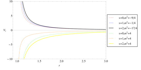
Figure 1: Behaviour of $V_{s}$ for a Schwarzschild-AdS₄ with $r_{h}=1$ in the three different wave states.

In Fig.(1) one can see that around the event horizon $V_{s}$ is always positive for the three wave states in the BF bound and it falls faster for s-wave than the other wave states when $r$ goes to infinity. For positive values of $m$ the potential $V_{s}$ becomes negative for the three wave states.

III Holographic superconductors in Hořava-Lifshitz gravity

In this section, we generalize the study of various holographic superconductors in the previous section to the Hořava-Lifshitz gravity. It is interesting to see how the breaking Lorentz invariance with $U(1)$ gauge symmetry may affect the properties of the superconductors. We note that the Hořava-Lifshitz gravity has been employed to investigate the s-wave holographic superconductors in Lin:2014bya ; Luo:2016ydt , also other applications of the AdS/CFT correspondence in condensate matter physics have been carried out Cai:2009hn ; Jing:2010dc ; Luo:2016zdo . In what follows, we extend our previous study to the p-wave and d-wave states while rewrite the equations of motion in an unified fashion.

III.1 An unified equations of motion for holographic superconductors

Due to the breaking of the symmetry between time and space in Hořava-Lifshitz gravity, it is convenient to describe the four dimensional spacetime in terms of the ADM metricGriffin:2012qx

$$ds^{2}=-N^{2}dt^{2}+\gamma_{ij}\left(dx^{i}+N^{i}dt\right)\left(dx^{j}+N^{j}dt\right),$$ (3.1)

where $i,j=1,2,3$, or equivalently, one has

$$g_{\mu\nu} = \left(\begin{array}[]{cc}g_{00}&g_{0j}\\ g_{i0}&g_{ij}\\ \end{array}\right)=\left(\begin{array}[]{cc}-N^{2}+N_{k}N^{k}&N_{j}\\ N_{i}&\gamma_{ij}\\ \end{array}\right),~{}~{}~{}g^{\mu\nu}=\left(\begin{array}[]{cc}g^{00}&g^{0j}\\ g^{i0}&g^{ij}\\ \end{array}\right)=\left(\begin{array}[]{cc}-\frac{1}{N^{2}}&\frac{N^{j}}{N^{2}}\\ \frac{N^{i}}{N^{2}}&\gamma^{ij}-\frac{N^{i}N^{j}}{N^{2}}\\ \end{array}\right).$$ (3.10)

In order to deal with a set of difficulties in HL gravity such as, strong coupling, instability, ghost mode and redundant parameters, it is found in HW4 that one may introduce a field $A$ with $U(1)$ gauge symmetry such that the action reads

$$S = \frac{1}{16\pi G}\int dtd^{3}xN\sqrt{\gamma}\left[{\cal L}_{K}-{\cal L}_{V}+{\cal L}_{A}+{\cal L}_{\varphi}+{\cal L}_{S}+16\pi G{\cal L}_{M}\right],$$ (3.11)

where

$${\cal L}_{K} = K_{ij}K^{ij}-\lambda K^{2},~{}~{}~{}{\cal L}_{V}=2\Lambda-\beta_{0}a_{i}a^{i}+\gamma_{1}R+{\cal L}_{V}^{H},$$

$${\cal L}_{A} = \frac{A}{N}(2\Lambda_{g}-R),~{}~{}~{}{\cal L}_{S}=\frac{A-{\cal A}}{N}\left(\sigma_{1}a_{i}a^{i}+\sigma_{2}a_{i}^{i}\right).$$ (3.12)

Here ${\cal L}_{V}^{H}$ represent the higher energy part of ${\cal L}_{V}$, and the coefficients $\lambda$, $\beta_{0}$, $\gamma_{1}$ $\sigma_{1}$ and $\sigma_{2}$ are all constants. ${\cal A}$ and ${\cal L}_{\varphi}$ are the functions of $\varphi$. One can choose the gauge $\varphi=0$ to eliminate these two terms. The term ${\cal L}_{M}$ is for the matter fields, which vanishes in the vacuum. Under these conditions a planar black hole solution of this HL gravity possesses the following form

$$N=\sqrt{f(r)},~{}~{}N^{i}=0,~{}~{}A=A_{0}\sqrt{f(r)},~{}~{}\gamma_{ij}=\left(\begin{array}[]{ccc}\frac{1}{f}&0&0\\ 0&r^{2}&0\\ 0&0&r^{2}\\ \end{array}\right),~{}~{}f=r^{2}-\frac{r_{h}^{3}}{r}$$ (3.16)

with $\beta_{0}=0,c_{1}=c_{2}$. Here we have chosen $\Lambda=\Lambda_{g}=-3$ without loss of generality.

In what follows, we study the holographic superconductor in the background metric of Eq.(3.16) in the probe limit. Since Eq.(3.16) does not consider the higher energy sector in the action, we will restrict our present study at the lower energy sector. According to Lin:2014bya , the Lagrangian for the matter fields read

$$\bar{{\cal L}}_{F} = -\frac{1}{4}\left\{-\frac{2}{N^{2}}\gamma^{ij}\left(F_{0i}-F_{ki}N^{k}\right)\left(F_{0j}-F_{lj}N^{l}\right)+\left(1+\eta_{0}+\eta_{A}\frac{A}{N}\right)F_{ij}F^{ij}\right\},$$

$$\bar{{\cal L}}_{S} = -\left\{-\frac{1}{N^{2}}\left[\partial_{t}\Psi-N^{k}\partial_{k}\Psi\right]^{2}+\left(1+\alpha_{0}+(\alpha_{A}-\alpha_{B})\frac{A}{N}\right)\left(\partial_{i}\Psi\right)\left(\partial^{i}\Psi\right)+\alpha_{A}\frac{\Psi}{N}A^{k}\partial_{k}\Psi+\alpha_{0}\Psi a^{i}\partial_{i}\Psi\right\},$$

$$\bar{{\cal L}}_{P} = -\frac{1}{2}\left\{-\frac{2}{N^{2}}\gamma^{ij}\left(\rho_{0i}-\rho_{ki}N^{k}\right)\left(\rho_{0j}-\rho_{lj}N^{l}\right)+\left(1+\xi_{0}+\xi_{A}\frac{A}{N}\right)\rho_{ij}\rho^{ij}\right\},$$

$$\bar{{\cal L}}_{D} = \frac{1}{N^{6}}\left(H_{0}-N^{l}H_{l}\right)^{2}-\frac{\gamma^{ij}}{N^{4}}H_{i}H_{j}-\frac{2\gamma^{lk}}{N^{2}}\left[\frac{1}{N^{2}}\left(H_{l0}-N^{m}H_{lm}\right)\left(H_{k0}-N^{n}H_{kn}\right)-\gamma^{ij}H_{li}H_{kj}\right]$$

$$+2E^{ijk}D_{k}B_{ij}+E^{ijk}E_{ijk}+\left(1+\gamma_{0}+\gamma_{A}\frac{A}{N}\right)\left(D_{k}B_{ij}\right)\left(D^{k}B^{ij}\right),$$

$$\bar{{\cal L}}_{C_{S}} = -\left[m_{S}^{2}+q^{2}(A_{t}-N^{k}A_{k})^{2}+\left(1+\alpha_{0}+(\alpha_{A}-\alpha_{B})\frac{A}{N}\right)A_{i}A^{i}\right]\Psi^{2},$$

$$\bar{{\cal L}}_{C_{P}} = -\left[m_{P}^{2}+q^{2}(A_{t}-N^{k}A_{k})^{2}+\left(1+\xi_{0}+\xi_{A}\frac{A}{N}\right)A_{i}A^{i}\right]\left[-\frac{(\rho_{t}-N^{k}\rho_{k})^{2}}{N^{2}}+\tau_{0}\rho^{i}\rho_{i}\right]$$

$$+iq\gamma\left[\bar{\gamma}\frac{\left(\rho_{t}-N^{k}\rho_{k}\right)^{2}}{N^{4}}N^{i}N^{j}+\tilde{\gamma}\frac{\rho_{t}-N^{k}\rho_{k}}{N^{2}}\left(N^{i}\rho^{j}+N^{j}\rho^{i}\right)+\rho^{i}\rho^{j}\right]F_{ij}$$

$$\bar{{\cal L}}_{C_{D}} = -\left[m_{D}^{2}+q^{2}(A_{t}-N^{k}A_{k})^{2}+\left(1+\gamma_{0}+\gamma_{A}\frac{A}{N}\right)A_{i}A^{i}\right]\left[\frac{\iota_{0}}{N^{4}}\left(B_{00}-2B_{0k}N^{k}+B_{ij}N^{i}N^{j}\right)^{2}\right.$$ (3.17)

$$\left.+\frac{2\iota}{N^{2}}\gamma^{ij}\left(B_{0i}+B_{il}N^{l}\right)\left(B_{0j}+B_{jk}N^{k}\right)+B_{ij}B^{ij}\right],$$

where

$$H_{\mu} = \nabla_{\mu}B_{00}-2N^{i}\nabla_{\mu}B_{0i}+N^{i}N^{j}\nabla_{\mu}B_{ij}$$

$$H_{i\mu} = \nabla_{\mu}B_{0i}-N^{k}\nabla_{\mu}B_{ik}$$

$$E_{ijk} = \frac{1}{N}\left[K_{ki}\left(B_{0j}-N^{l}B_{lj}\right)+K_{kj}\left(B_{0i}-N^{k}B_{ki}\right)\right]$$

$$F_{0i} = \partial_{t}A_{i}-\partial_{i}A_{t}$$

$$\rho_{0i} = \partial_{t}\rho_{i}-\partial_{i}\rho_{t}.$$ (3.18)

Moreover, we removed odd power terms from the Lagrangian in order to guarantee that the resulting equations of motion are homogeneous.

The actions for the s-wave, p-wave and d-wave holographic superconductors in HL gravity are

$$\bar{S}_{S} = \frac{1}{16\pi G}\int dtd^{3}xN\sqrt{\gamma}\left[\bar{\cal L}_{F}+\bar{\cal L}_{S}+\bar{\cal L}_{C_{S}}\right],$$ (3.19)

$$\bar{S}_{P} = \frac{1}{16\pi G}\int dtd^{3}xN\sqrt{\gamma}\left[\bar{\cal L}_{F}+\bar{\cal L}_{P}+\bar{\cal L}_{C_{P}}\right],$$ (3.20)

$$\bar{S}_{D} = \frac{1}{16\pi G}\int dtd^{3}xN\sqrt{\gamma}\left[\bar{\cal L}_{F}+\bar{\cal L}_{D}+\bar{\cal L}_{C_{D}}\right],$$ (3.21)

respectively, from which the coupled equations of motion can be derived.

In order to derive the equations of motion, we adopt the same Ansatz as before, namely, $A_{\nu}=\delta^{t}_{\nu}\phi(r)$, $\Psi=\psi_{S}(r)$, $\rho_{\mu}=\delta_{\mu}^{x}\rho_{x}(r)=\delta_{\mu}^{x}r\psi_{P}$ and $B_{\mu\nu}=(\delta_{\mu}^{x}\delta_{\nu}^{x}-\delta_{\mu}^{y}\delta_{\nu}^{y})\frac{r^{2}}{\sqrt{2}}\psi_{D}(r)$. Also, to write down the equations of motion for different wave states in an unified fashion, we introduce transformations of the fields and definitions of the parameters in the actions given by the Eqs.(3.19), (3.20) and (3.21) as follows

• transformations in the action Eq.(3.19) for s-wave superconductor:

  $$\phi \rightarrow \frac{1+\alpha_{0}+A_{0}(\alpha_{A}-\alpha_{B})}{q}\phi,~{}~{}\psi\rightarrow\frac{\psi}{q},$$

  $$\alpha_{A} \rightarrow \frac{4\alpha(1+\beta)(1+\eta_{0}+A_{0}\eta_{A})-\alpha_{0}}{A_{0}},~{}~{}~{}\alpha_{B}\rightarrow\frac{(4\alpha(1+\beta)-\beta)(a+\eta_{0}+A_{0}\eta_{A})-\eta_{0}-A_{0}\eta_{A}}{A_{0}},$$

  $$\omega \rightarrow \sqrt{1+\eta_{0}+A_{0}\eta_{A}},~{}~{}~{}m\rightarrow m\sqrt{(1+\beta)(1+\eta_{0}+A_{0}\eta_{A})};$$ (3.22)

• transformations in the action Eq.(3.20) for p-wave superconductor:

  $$\phi \rightarrow \frac{1+\xi_{0}+A_{0}\xi_{A}}{q}\phi,~{}~{}~{}\psi\rightarrow\frac{\psi}{q},~{}~{}~{}\eta_{A}\rightarrow\frac{A_{0}\xi_{A}+\xi_{0}-\eta_{0}-\beta-\beta\eta_{0}}{A_{0}(1+\beta)},$$

  $$\omega \rightarrow \sqrt{\frac{1+\xi_{0}+A_{0}\xi_{A}}{1+\beta}},~{}~{}~{}m\rightarrow m\sqrt{(1+\beta)(1+\xi_{0}+A_{0}\xi_{A})};$$ (3.23)

• transformations in the action Eq.(3.21) for d-wave superconductor:

  $$\phi \rightarrow \frac{1+\gamma_{0}-\gamma_{A}A_{0}\xi_{A}}{q}\phi,~{}~{}~{}\psi\rightarrow\frac{\psi}{q},~{}~{}~{}\gamma_{0}\rightarrow\eta_{0}+A_{0}\left(\eta_{A}-\gamma_{A}\right)+\beta(1+\eta_{0}+A_{0}\eta_{A}),$$

  $$\omega \rightarrow \sqrt{1+\eta_{0}+A_{0}\eta_{A}},~{}~{}m\rightarrow m\sqrt{(1+\beta)\left(1+\eta_{0}+A_{0}\eta_{A}\right)}.$$ (3.24)

After somewhat tedious but straightforward calculations, one obtains the following unified equation of motion in Hořava-Lifshitz gravity

$$\psi^{\prime\prime}+\left(\frac{f^{\prime}}{f}+\frac{2}{r}\right)\psi^{\prime}+\left(\frac{\phi^{2}}{f^{2}}+\bar{V}_{s}(r)\right)\psi = 0,$$ (3.25a)

$$\phi^{\prime\prime}+\frac{2}{r}\phi^{\prime}-\frac{2\psi^{2}}{f}\phi = 0,$$ (3.25b)

$$A_{x}^{\prime\prime}+\frac{f^{\prime}}{f}A_{x}^{\prime}+\left(\frac{\omega^{2}}{f^{2}}-2(1+\beta)\frac{\psi^{2}}{f}\right)A_{x} = 0.$$ (3.25c)

where the effective potential is

$$\bar{V}_{s}(r)=-\frac{m^{2}}{f}+(2-s)(s+(1-s)\alpha)\frac{f^{\prime}}{rf}+\frac{\alpha}{2}(2-s)(1-s)\frac{f^{\prime\prime}}{f}+\frac{s(1-s)}{r^{2}}.$$ (3.26)

Here, similarly to the case in Einstein gravity, $s=0,1,2$ correspond to s-wave, p-wave and d-wave holographic superconductors, respectively. The terms related to $\alpha$ and $\beta$ indicate the effects of the breaking Lorentz invariance in Hořava-Lifshitz gravity. In other words, the holographic setup in Einstein gravity is restored with $\alpha=\beta=0$. Additionally, inspecting the Eq.(3.26) one can see that only the s-wave state $(s=0)$ is sensitive to $\alpha$.

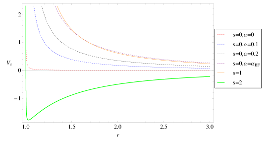
Figure 2: Behaviour of $V_{s}$ for a black hole in HL gravity with $r_{h}=1,m^{2}_{BF}=-0.01,$ in the three different wave states. For this value of the squared mass $\alpha_{BF}=\frac{28}{75}$.

In Fig.(2) one can observe that the behavior of the effective potential for the s-wave state with $\alpha_{BF}$ and p-wave state is quite similar. From the Eqs.($\ref{31a},\ref{32}$) the BF bound for the planar black hole in HL gravity can be obtained for each wave state and results in a more complex relation. It is

$$m^{2}_{BF}=-\frac{9}{4}+5s-3s^{2}+6\alpha-9s\alpha+3s^{2}\alpha.$$ (3.27)

In general the BF bound is a negative value for the squared mass of the scalar field, however for the s-wave state this limit becomes positive at critical value $\alpha_{c}>\frac{3}{8}$ and increases linearly with $\alpha$. For d-wave and p-wave this bound is not affected by $\alpha$ as one can viewed in Fig.(3).

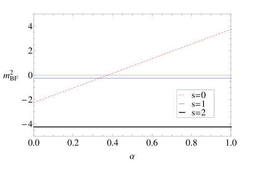
Figure 3: Breitenlohner-Freedman bound for s-wave $(m^{2}_{BF}=-\frac{9}{4}+6\alpha)$, p-wave $(m^{2}_{BF}=-\frac{1}{4})$ and d-wave $(m^{2}_{BF}=-\frac{17}{4})$ states.

III.2 Numerical results on the condensation and the optical conductivity

Now we are in position to solve the equations of motion Eqs.(3.25a-3.25c) and to numerically study the condensation and the conductivity of the superconductors.

Considering the background metric Eq.(3.16), the boundary conditions of Eqs.(3.25a-3.25c) read

$$\phi = \mu+\frac{\rho}{r},$$

$$\psi = \psi_{1}r^{-(3-\Delta)/2}+\psi_{2}r^{-(3+\Delta)/2},$$

$$A_{x} = a_{0}+\frac{a_{1}}{r},$$ (3.28)

where $\Delta$ satisfies

$$\Delta^{2}=9+4m^{2}-24\alpha-4s(5-3s+3s\alpha-9\alpha).$$ (3.29)

According to gauge/gravity duality, $\mu$ and $\rho$ are interpreted as the chemical potential and the charge density of the theory on the boundary. Either $\psi_{1}$ or $\psi_{2}$ can be the source of the dual operator, and therefore must take to be zero, while the other one is related to the vacuum expectation value of the dual operator $<O_{i}>\sim\psi_{i}(i=1,2)$. The optical conductivity can be read off from the asymptotic behavior of $A_{x}$ as

$$\sigma(\omega)=\frac{a_{1}}{i\omega a_{0}}.$$ (3.30)

Near the horizon, the regular condition implies that $\phi(r\to r_{h})=0$ while $\psi(r\to r_{h})=finite$, and the equation of motion gives $A_{x}(r\to r_{h})\sim f^{\pm\frac{i\omega}{f^{\prime}(r_{h})}}$ among which we will choose the infalling solution with the minus sign. The equations then can be numerically integrated from the horizon to the boundary via the shooting method.

We note one may rewrite Eq.(3.26) by substituting $m$ in favor of $\Delta$ defined by Eq.(3.29) as follows,

$$\bar{V}_{s}(r)=-\frac{(\Delta^{2}-9)r^{3}-4r_{h}^{3}s}{4r^{2}(r^{3}-r_{h}^{3})}.$$ (3.31)

Before numerically solving the equations, we give several remarks on the properties of the system. Firstly, Eq.(3.31) indicates that the equation of motion can be view as not explicitly dependent on the value of $\alpha$, which measures the corrections of Hořava-Lifshitz theory. In the next section, however, we will see that the critical temperature depends on $\alpha$.

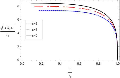
Figure 4: Condensation curves $\psi\sim r^{-(3+\Delta)/2}$ for $\Delta=1$.

Therefore, for a given $\alpha$ in Hořava-Lifshitz gravity, one can always find a corresponding system in Einstein gravity by tuning the value of $m$, so that the properties of condensate curve are the same. However, since $\beta$ appears in Eq.(3.25c), the conductivity of the two systems remains different.

The numerical results for various holographic superconductors are in Figs.4-7.

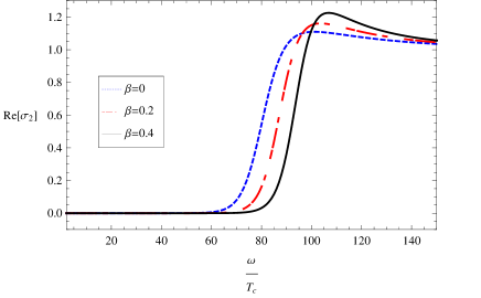
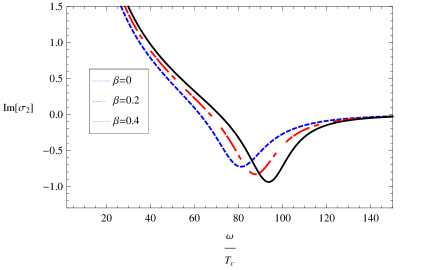
Figure 5: Conductivity for $\Delta=1$, $s=0$, and $\psi\sim r^{-(3+\Delta)/2}$ at infinity.

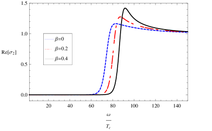
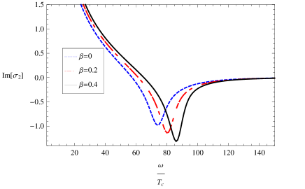
Figure 6: Conductivity for $\Delta=1$, $s=1$ and $\psi\sim r^{-(3+\Delta)/2}$ at infinity.

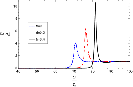
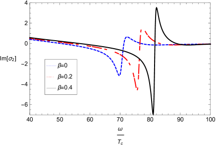
Figure 7: Conductivity for $\Delta=1$, $s=2$ and $\psi\sim r^{-(3+\Delta)/2}$ at infinity.

In Fig.4, we present the condensation of the matter field with $\Delta=1$ by solving Eqs.(3.25a) and (3.25b). We study the condensate of $<O_{2}>$ by taking $\psi_{1}=0$ because as addressed in Hartnoll:2008kx , the condensate of $<O_{1}>$ is unstable due to its tendency of divergence when the temperature approaches to zero.

Moreover, we show the results of optical conductivity $\sigma$ in Figs.5-7, which correspond to the behavior for s-wave, p-wave and d-wave superconducting phases, respectively. From Eq.(3.25c), one sees that the conductivity depends on the parameter $\beta$, which measures the breaking of the Lorentz invariance. We observe that, as $\beta$ increases, the ratio between energy gap and the critical temperature also increases. This result agrees well with the observation in the s-wave superconductor investigated in Lin:2014bya ; Luo:2016ydt .

III.3 Semi-analytical results on the condensation

In order to gain a better understanding of the influence of the HL gravity in holographic superconductor scenario, we have calculated a semi-analytical expression for the vacuum expectation value of the dual operator $<O_{i}>$ following the approach developed in Gregory:2009fj ; Pan:2009xa . Matching the asymptotic solution for $\phi(r)$ and $\psi(r)$ and their derivatives in an arbitrary point $z_{m}=\frac{r_{h}}{r_{m}}$ we get the following expression for the expectation value $<\mathcal{O}_{i}>$ as

$$\left<\mathcal{O}_{i}\right> = \Pi~{}T^{\lambda_{i}}\left(\frac{T_{c}}{T}\right)\sqrt{1-\frac{T}{T_{c}}}\sqrt{1+\frac{T}{T_{c}}}$$ (3.32)

where $\Pi$ is defined by

$$\Pi = \left(\frac{z_{m}^{-\lambda_{i}+1}\left(2-\sigma(1-z_{m})\right)}{\lambda_{i}(1-z_{m})+2z_{m}}\right)\sqrt{\frac{3}{2(1-z_{m})}}\left(\frac{4\pi}{3}\right)^{\lambda_{i}}$$ (3.33)

and $\sigma$ and $\lambda_{i}$ as

$$\sigma = \alpha(2-s)(1-s)+s(2-s)-\frac{m^{2}}{3}$$ (3.35)

$$\lambda_{i} = \frac{3}{2}\pm\frac{\Delta}{2}$$ (3.36)

The expression for the critical temperature $T_{c}$ is given by

$$T_{c} = \frac{3}{4\pi}\sqrt{\frac{\rho}{6}\sqrt{\frac{2}{\Sigma}}}$$ (3.37)

$$\Sigma = \frac{s}{2}+\frac{\sigma(\sigma-2)}{2}-\frac{\sigma}{1-z_{m}}+\frac{\lambda_{i}(2-\sigma(1-z_{m}))}{\lambda_{i}(1-z_{m})+2z_{m}}\left(\frac{1}{1-z_{m}}\right)$$ (3.38)

The results presented in the Eqs.(3.32,3.37) generalize that one in Gregory:2009fj for $2+1$ holographic superconductor.

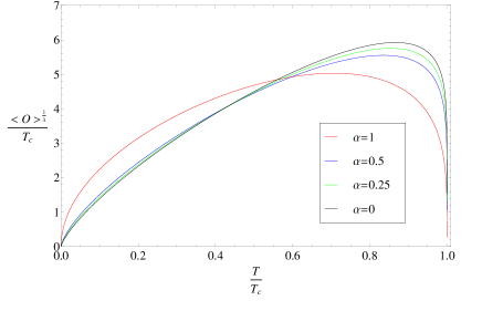
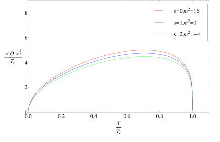
Figure 8: Condensation curves obtained from the Eq.(3.32) for some values of $\alpha$ and $z_{m}=1/2$ for s-wave state superconductor (Left) and for the three wave states with $\alpha=3$ (Right).

In Fig.(8) one observes that the Eq.(3.32) fails in describing the behavior of the condensate when $T\to 0$. However near to the critical temperature $T_{c}$ the mean field theory results $<\mathcal{O}_{i}>\sim\sqrt{1-\frac{T}{T_{c}}}$ is recovered. For the s-wave state, the condensation becomes easier when $\alpha$ increases. For the p-wave and d-wave states the condensation is not affected by $\alpha$. Thus, looking at only the phase transition curves the s-wave state is the only one that has a detectable influence of the HL gravity. Comparing the condensation among the three wave states one can see that a d-wave superconductor condensates at the highest temperature.

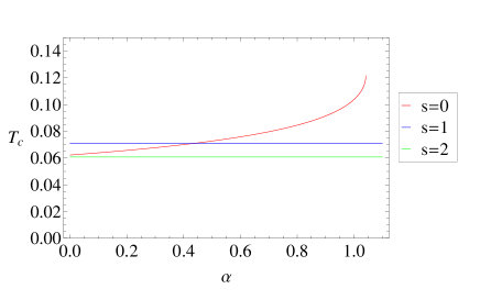
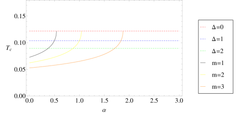
Figure 9: Dependence of the critical temperature $T_{c}$ on $\alpha$ with $m=2$ for all three wave states (Left) and for some values of mass $m$ and $\Delta$ for the s-wave state (Right).

In Fig.(9) one can see that just as in BF bound, the critical temperature is independent of $\alpha$ for the d-wave and p-wave states. In general, $T_{c}$ has an upper bound with $\alpha$ for the s-wave state. The horizontal lines show the values of $T_{c}$ when $\Delta=0,1,2$.

IV Concluding remarks

In summary, in this work, we study the s-wave, p-wave, and d-wave holographic superconductors dual to a planar black hole in Hořava-Lifshitz gravity. For the models discussed in the present work, we manage to rewrite the equations of motion into an unified form. Numerical and semi-analytical calculations are carried out and condensations are found for all three holographic superconductors with different wave states. The s-wave superconductors suffer the strongest influence of HL gravity parameters. Thus, they could be used to test the Lorentz symmetry breaking. However, the present study is limited to the case of planar AdS background, a more general metric may likely lead to more divergent results. We did neither consider the backreaction of the matter field, which also may imply additional nontrivial effects owing to the breaking of Lorentz invariance. Lastly, we have only discussed the lower energy sector. As a result, many effects such as superluminal particle and universal horizon lay beyond the scope of the current study. Nonetheless, the calculated results show that the parameter $\beta$ plays a distinct role in the properties of the optical conductivity even for a rather simple metric. Hořava-Lifshitz gravity is one of the theories that successfully passes all the observable post-Newtonian test via solar data. In this context, the findings of the present work somewhat indicate that the measured optical conductivity can be utilized to quantify the breaking of Lorentz invariance, and therefore shed some light on further discrimination between different theories.

References

- (1) J. M. Maldacena, “The large N limit of superconformal field theories and supergravity,” Adv. Theor. Math. Phys. 2 (1998) 231 [Int. J. Theor. Phys. 38 (1999) 1113].
- (2) S. S. Gubser, I. R. Klebanov and A. M. Polyakov, “A semiclassical limit of the gauge string correspondence,” Nucl. Phys. B 636 (2002) 99.
- (3) E. Witten, “Anti-de Sitter space and holography, ” Adv. Theor. Math. Phys. 2 (1998) 253.
- (4) Maldacena, Juan. “The Large N limit of superconformal field theories and supergravity”. Advances in Theoretical and Mathematical Physics. 2, 231 (1998), arXiv:hep-th/9711200.
- (5) S. A. Hartnoll, C. P. Herzog and G. T. Horowitz, “Building a Holographic Superconductor,” Phys. Rev. Lett. 101, 031601 (2008) [arXiv:0803.3295 [hep-th]].
- (6) S. A. Hartnoll, C. P. Herzog and G. T. Horowitz, “Holographic Superconductors,” JHEP 0812, 015 (2008) [arXiv:0810.1563 [hep-th]].
- (7) T. Albash and C. V. Johnson, “A Holographic Superconductor in an External Magnetic Field,” JHEP 0809, 121 (2008) [arXiv:0804.3466 [hep-th]].
- (8) C. P. Herzog, P. K. Kovtun and D. T. Son, “Holographic model of superfluidity,” Phys. Rev. D 79, 066002 (2009) [arXiv:0809.4870 [hep-th]].
- (9) T. Albash and C. V. Johnson, “Vortex and Droplet Engineering in Holographic Superconductors,” Phys. Rev. D 80, 126009 (2009) [arXiv:0906.1795 [hep-th]].
- (10) R. Gregory, S. Kanno and J. Soda, “Holographic Superconductors with Higher Curvature Corrections,” JHEP 0910, 010 (2009) [arXiv:0907.3203 [hep-th]].
- (11) R. A. Konoplya and A. Zhidenko, “Holographic conductivity of zero temperature superconductors,” Phys. Lett. B 686, 199 (2010) [arXiv:0909.2138 [hep-th]].
- (12) S. Franco, A. M. Garcia-Garcia and D. Rodriguez-Gomez, “A Holographic approach to phase transitions,” Phys. Rev. D 81, 041901 (2010) [arXiv:0911.1354 [hep-th]].
- (13) S. Chen, L. Wang, C. Ding and J. Jing, “Holographic superconductors in the AdS black hole spacetime with a global monopole,” Nucl. Phys. B 836, 222 (2010) [arXiv:0912.2397 [gr-qc]].
- (14) Q. Pan, B. Wang, E. Papantonopoulos, J. Oliveira and A. B. Pavan, “Holographic Superconductors with various condensates in Einstein-Gauss-Bonnet gravity,” Phys. Rev. D 81, 106007 (2010) [arXiv:0912.2475 [hep-th]].
- (15) X. H. Ge, B. Wang, S. F. Wu and G. H. Yang, “Analytical study on holographic superconductors in external magnetic field,” JHEP 1008, 108 (2010) [arXiv:1002.4901 [hep-th]].
- (16) D. Momeni, M. R. Setare and N. Majd, “Holographic superconductors in a model of non-relativistic gravity,” JHEP 1105, 118 (2011) [arXiv:1003.0376 [hep-th]].
- (17) Y. Liu and Y. W. Sun, “Holographic Superconductors from Einstein-Maxwell-Dilaton Gravity,” JHEP 1007, 099 (2010) [arXiv:1006.2726 [hep-th]].
- (18) Y. S. Myung and C. Park, “Holographic superconductor in the exact hairy black hole,” Phys. Lett. B 704, 242 (2011) [arXiv:1007.0816 [hep-th]].
- (19) Y. Liu, Q. Pan, B. Wang and R. G. Cai, “Dynamical perturbations and critical phenomena in Gauss-Bonnet-AdS black holes,” Phys. Lett. B 693, 343 (2010) [arXiv:1007.2536 [hep-th]].
- (20) X. M. Kuang, W. J. Li and Y. Ling, “Holographic Superconductors in Quasi-topological Gravity,” JHEP 1012, 069 (2010) [arXiv:1008.4066 [hep-th]].
- (21) L. Barclay, R. Gregory, S. Kanno and P. Sutcliffe, “Gauss-Bonnet Holographic Superconductors,” JHEP 1012, 029 (2010) [arXiv:1009.1991 [hep-th]].
- (22) J. P. Wu, Y. Cao, X. M. Kuang and W. J. Li, “The 3+1 holographic superconductor with Weyl corrections,” Phys. Lett. B 697, 153 (2011) [arXiv:1010.1929 [hep-th]].
- (23) R. Flauger, E. Pajer and S. Papanikolaou, “A Striped Holographic Superconductor,” Phys. Rev. D 83, 064009 (2011) [arXiv:1010.1775 [hep-th]].
- (24) R. G. Cai, H. F. Li and H. Q. Zhang, “Analytical Studies on Holographic Insulator/Superconductor Phase Transitions,” Phys. Rev. D 83, 126007 (2011) [arXiv:1103.5568 [hep-th]].
- (25) Y. Peng, Q. Pan and B. Wang, “Various types of phase transitions in the AdS soliton background,” Phys. Lett. B 699, 383 (2011) [arXiv:1104.2478 [hep-th]].
- (26) W. J. Li, Y. Tian and H. b. Zhang, “Periodically Driven Holographic Superconductor,” JHEP 1307 (2013) 030 [arXiv:1305.1600 [hep-th]].
- (27) X. M. Kuang, E. Papantonopoulos, G. Siopsis and B. Wang, “Building a Holographic Superconductor with Higher-derivative Couplings,” Phys. Rev. D 88, 086008 (2013) [arXiv:1303.2575 [hep-th]].
- (28) D. Roychowdhury, “Effect of external magnetic field on holographic superconductors in presence of nonlinear corrections,” Phys. Rev. D 86, 106009 (2012) [arXiv:1211.0904 [hep-th]].
- (29) Z. Fan, “Holographic superconductors with hyperscaling violation,” JHEP 1309, 048 (2013) [arXiv:1305.2000 [hep-th]].
- (30) A. Dey, S. Mahapatra and T. Sarkar, “Generalized Holographic Superconductors with Higher Derivative Couplings,” JHEP 1406, 147 (2014) [arXiv:1404.2190 [hep-th]].
- (31) Y. Ling, P. Liu, C. Niu, J. P. Wu and Z. Y. Xian, “Holographic Superconductor on Q-lattice,” JHEP 1502, 059 (2015) [arXiv:1410.6761 [hep-th]].
- (32) J. W. Lu, Y. B. Wu, P. Qian, Y. Y. Zhao and X. Zhang, “Lifshitz Scaling Effects on Holographic Superconductors,” Nucl. Phys. B 887 (2014) 112 [arXiv:1311.2699 [hep-th]].
- (33) X. M. Kuang and E. Papantonopoulos, “Building a Holographic Superconductor with a Scalar Field Coupled Kinematically to Einstein Tensor,” JHEP 1608, 161 (2016) [arXiv:1607.04928 [hep-th]].
- (34) C. C. Tsuei and J. R. Kirtley, Rev. Mod. Phys. 72, 969 (2000).
- (35) S. S. Gubser and S. S. Pufu, “The Gravity dual of a p-wave superconductor,” JHEP 0811, 033 (2008) [arXiv:0805.2960 [hep-th]].
- (36) R. G. Cai, S. He, L. Li and L. F. Li, “A Holographic Study on Vector Condensate Induced by a Magnetic Field,” JHEP 1312, 036 (2013) [arXiv:1309.2098 [hep-th]].
- (37) A. Donos and J. P. Gauntlett, “Holographic helical superconductors,” JHEP 1112, 091 (2011) [arXiv:1109.3866 [hep-th]].
- (38) J. W. Chen, Y. J. Kao, D. Maity, W. Y. Wen and C. P. Yeh, “Towards A Holographic Model of D-Wave Superconductors,” Phys. Rev. D 81, 106008 (2010) [arXiv:1003.2991 [hep-th]].
- (39) F. Benini, C. P. Herzog, R. Rahman and A. Yarom, “Gauge gravity duality for d-wave superconductors: prospects and challenges,” JHEP 1011, 137 (2010) [arXiv:1007.1981 [hep-th]].
- (40) H. B. Zeng, Z. Y. Fan and H. S. Zong, “d-wave Holographic Superconductor Vortex Lattice and Non-Abelian Holographic Superconductor Droplet,” Phys. Rev. D 82, 126008 (2010) [arXiv:1007.4151 [hep-th]].
- (41) X. H. Ge, S. F. Tu and B. Wang, “d-Wave holographic superconductors with backreaction in external magnetic fields,” JHEP 1209, 088 (2012) [arXiv:1209.4272 [hep-th]].
- (42) K. Y. Kim and M. Taylor, “Holographic d-wave superconductors,” JHEP 1308, 112 (2013) [arXiv:1304.6729 [hep-th]].
- (43) M. Nishida, “Phase Diagram of a Holographic Superconductor Model with s-wave and d-wave,” JHEP 1409, 154 (2014) [arXiv:1403.6070 [hep-th]].
- (44) L. F. Li, R. G. Cai, L. Li and Y. Q. Wang, “Competition between s-wave order and d-wave order in holographic superconductors,” JHEP 1408, 164 (2014) [arXiv:1405.0382 [hep-th]].
- (45) A. Krikun, “Phases of holographic d-wave superconductor,” JHEP 1510, 123 (2015) [arXiv:1506.05379 [hep-th]].
- (46) G. T. Horowitz, “Introduction to Holographic Superconductors,” Lect. Notes Phys. 828, 313 (2011), [arXiv:1002.1722 [hep-th]].
- (47) R. G. Cai, L. Li, L. F. Li and R. Q. Yang, “Introduction to Holographic Superconductor Models,” Sci. China Phys. Mech. Astron. 58, no. 6, 060401 (2015), [arXiv:1502.00437 [hep-th]].
- (48) P. Horava, “Quantum Gravity at a Lifshitz Point,” Phys. Rev. D 79, 084008 (2009) [arXiv:0901.3775 [hep-th]].. “General Covariance in Quantum Gravity at a Lifshitz Point,” Phys. Rev. D 82, 064027 (2010) [arXiv:1007.2410 [hep-th]].
- (49) K. Lin, A. Wang, Q. Wu and T. Zhu, “On strong coupling in nonrelativistic general covariant theory of gravity,” Phys. Rev. D 84, 044051 (2011) [arXiv:1106.1486 [hep-th]].
- (50) T. Zhu, Q. Wu, A. Wang and F. W. Shu, “U(1) symmetry and elimination of spin-0 gravitons in Hořava-Lifshitz gravity without the projectability condition,” Phys. Rev. D 84, 101502 (2011) [arXiv:1108.1237 [hep-th]].
- (51) K. Lin, S. Mukohyama, A. Wang and T. Zhu, “Post-Newtonian approximations in the Hořava-Lifshitz gravity with extra U(1) symmetry,” Phys. Rev. D 89, no. 8, 084022 (2014) [arXiv:1310.6666 [hep-ph]].
- (52) K. Lin, W. L. Qian and A. B. Pavan, “Scalar quasinormal modes of anti-de Sitter static spacetime in Hořava-Lifshitz gravity with symmetry,” Phys. Rev. D 94, no. 6, 064050 (2016) [arXiv:1609.05963 [gr-qc]].
- (53) K. Lin, E. Abdalla and A. Wang, “Holographic superconductors in Hořava-Lifshitz gravity,” Int. J. Mod. Phys. D 24, no. 06, 1550038 (2015) [arXiv:1406.4721 [hep-th]].
- (54) C. J. Luo, X. M. Kuang and F. W. Shu, “Lifshitz holographic superconductor in Hořava-Lifshitz gravity,” Phys. Lett. B 759, 184 (2016) [arXiv:1605.03260 [hep-th]].
- (55) R. G. Cai and H. Q. Zhang, “Holographic Superconductors with Hořava-Lifshitz Black Holes,” Phys. Rev. D 81, 066003 (2010) [arXiv:0911.4867 [hep-th]].
- (56) J. Jing, L. Wang and S. Chen, “Holographic Superconductors in z = 3 Hořava-Lifshitz Gravity without condition of detailed balance,” arXiv:1001.1472 [hep-th].
- (57) C. J. Luo, X. M. Kuang and F. W. Shu, “Charged Lifshitz black hole and probed Lorentz-violation fermions from holography,” Phys. Lett. B 769, 7 (2017) [arXiv:1612.01247 [hep-th]].
- (58) T. Griffin, P. Hořava and C. M. Melby-Thompson, “Lifshitz Gravity for Lifshitz Holography,” Phys. Rev. Lett. 110, no. 8, 081602 (2013) [arXiv:1211.4872 [hep-th]].