Ground state properties of interacting Bose polarons

Abstract

We theoretically investigate the role of multiple impurity atoms on the ground state properties of Bose polarons. The Bogoliubov approximation is applied for the description of the condensate resulting in a Hamiltonian containing terms beyond the Fröhlich approximation. The many-body nature of the impurity atoms is taken into account by extending the many-body description for multiple Fröhlich polarons, revealing the static structure factor of the impurities as the key quantity. Within this formalism various experimentally accessible polaronic properties are calculated such as the energy and the effective mass. These results are examined for system parameters corresponding to two recent experimental realizations of the Bose polaron, one with fermionic impurities and one with bosonic impurities.

I Introduction

In general the complexity of many-body quantum systems makes it very hard to make exact predictions starting from a microscopic model. In order to deal with these systems one typically has to rely on approximations and an example with a particularly appealing physical interpretation is the notion of quasiparticles. They behave as effectively free particles but with properties that depend on the many-body nature of the system. An example of such a quasiparticle which has attracted a lot of interest over the years is the polaron. Its popularity can be partly explained by its conceptual simplicity. The polaron was introduced by Landau in 1933 for the description of an electron in a charged lattice Landau (1933). In this picture the quasiparticle corresponds to the electron together with its surrounding cloud of lattice polarization. Fröhlich derived a microscopic Hamiltonian for the polaron in terms of the electron interacting with the lattice vibrations or phonons of the crystal Fröhlich (1954). Various approximations and numerical approaches have been applied to calculate the ground state properties of the Fröhlich Hamiltonian (see Devreese (2010) for a detailed review). A variational approach was developed by Lee, Low and Pines which is based on a unitary transformation removing the electron degrees of freedom and which is valid at weak and intermediate polaronic coupling Lee et al. (1953). This approach was later extended by Brosens, Lemmens, and Devreese in Ref. Lemmens et al. (1977) to examine the effect of multiple interacting electrons which was incorporated through the static structure factor.

More recently it has been realized that ultracold gases can be used as an experimental platform to probe polaronic physics. Different classes of polarons have been considered such as the Fermi polaron which corresponds to an impurity atom in a quantum degenerate fermionic gas Schirotzek et al. (2009); Koschorreck et al. (2012). Another example, on which we will focus in this paper, is an impurity atom immersed in a Bose condensed gas (see Ref. Grusdt and Demler (2015) for a review). This realization has led to a revival of the Fröhlich Hamiltonian since under certain conditions the same polaron Hamiltonian applies as originally derived by Fröhlich for the description of an electron in a charged lattice Kalas and Blume (2006); Cucchietti and Timmermans (2006); Tempere et al. (2009). Within this mapping the role of the electron is played by the impurity and the phonons are replaced by the Bogoliubov excitations. This allowed to apply various theoretical approaches that were originally developed for the solid state Fröhlich polaron to the Bose polaron. For example the extension of the Lee-Low-Pines approach for multiple electrons was applied to multiple impurity atoms in a Bose-Einstein condensate in Ref. Casteels et al. (2011a) for fermionic impurities and in Ref. Casteels et al. (2013) for bosonic impurities.

The applicability of the Fröhlich Hamiltonian for the Bose polaron can only be justified for weak interactions between the impurity and the bosons Blinova et al. (2013). In recent years much effort has been devoted towards the experimental realization of the Bose polaron Nascimbène et al. (2009); Heinze et al. (2011); Will et al. (2011); Catani et al. (2012); Hohmann et al. (2015); Rentrop et al. (2016) and recently two set-ups have been presented that measure the polaron energy and linewidth through RF-spectroscopy, one with fermionic impurities Hu et al. (2016) and one with bosonic impurities Jørgensen et al. (2016). These experiments apply a Feshbach resonance to tune the impurity-boson scattering length, allowing to probe the system in the whole range from weak to strong coupling. This revealed that the Fröhlich Hamiltonian is not adequate to describe all the different regimes, especially in the regime of large impurity-boson scattering length. Considering certain terms in the Hamiltonian that are neglected within the Fröhlich approximation leads to a much better agreement with the experimental observations Levinsen et al. (2015); Shchadilova et al. (2016); Grusdt et al. (2017); Camacho-Guardian and Bruun (2018).

In this paper we present a first step towards the description of a gas of interacting Bose polarons beyond weak coupling. The descriptions that go beyond the Fröhlich approximation mostly consider just a single impurity. However in the recent experimental set-ups presented in Refs. Hu et al. (2016); Jørgensen et al. (2016) multiple impurities are present with an appreciable density. We will extend the Lee-Low-Pines many-body approach to multiple Fröhlich polarons to the Hamiltonian that contains the additional beyond Fröhlich terms. We find that, as for the usual Fröhlich polaron, the structure factor of the impurities is the key ingredient needed to incorporate the effect of multiple impurities. We use this to calculate experimentally relevant properties such as the polaron energy and the effective mass. These results are then examined for the system parameters corresponding to the experiments of Refs. Hu et al. (2016); Jørgensen et al. (2016) and the deviations from the single polaron results are discussed.

The paper starts with introducing the Hamiltonian for the Bose polaron in section II and applying the Lee-Low-Pines approximation for multiple impurities. In this section the analytical results for the polaron energy and the effective mass are also presented. Then, in section III, the two recent experimental realizations of the Bose polaron are discussed with an emphasis on the system parameters. Section IV examines the results for the parameters corresponding to these two experimental systems. Finally, in section V, we present the main conclusions and perspectives.

II Gas of Bose Polarons

We start from the microscopic Hamiltonian of a gas of bosons interacting with impurities:

$$\hat{H}= \sum_{\bf{k}}\left(\epsilon_{k}-\mu\right)\hat{b}^{\dagger}_{\bf{k}}\hat{b}_{\bf{k}}+\frac{1}{2}\sum_{\bf{k},\bf{k}^{\prime},\bf{q}}V_{BB}\left(\bf{q}\right)\hat{b}^{\dagger}_{\bf{k}^{\prime}-\bf{q}}\hat{b}^{\dagger}_{\bf{k}+\bf{q}}\hat{b}_{\bf{k}}\hat{b}_{\bf{k}^{\prime}}+\sum_{i}^{N_{I}}\frac{\hat{p}^{2}_{i}}{2m_{I}}+\sum_{i<j}^{N_{I}}U\left(\hat{\bf{r}}_{i}-\hat{\bf{r}}_{j}\right)$$

$$+\sum_{\bf{k},\bf{q}}V_{IB}\left(\bf{q}\right)\hat{\rho}_{\bf{q}}\hat{b}^{\dagger}_{\bf{k}-\bf{q}}\hat{b}_{\bf{k}}$$ (1)

The first two terms describe the bosons with chemical potential $\mu$, mass $m_{B}$, kinetic energy $\epsilon_{k}=\hbar^{2}k^{2}/(2m_{B})$ and $V_{BB}\left(\bf{q}\right)$ the Fourier transform of the interaction amplitude. The creation (annihilation) operators for the bosons are $\{\hat{b}^{\dagger}_{\bf{k}}\}$ ($\{\hat{b}_{\bf{k}}\}$). The next two terms describe the impurities with mass $m_{I}$ and momentum (position) operators $\{\hat{\bf{p}}_{i}\}$ ($\{\hat{\bf{r}}_{i}\}$). The impurity-impurity interaction potential is $U(r)$. The last term gives the interaction between the bosons and the impurities with $V_{IB}\left(\bf{q}\right)$ the Fourier transform of the interaction amplitude and $\hat{\rho}_{\bf{q}}=\sum_{i}^{N_{I}}e^{\mathrm{i}{\bf{q}}.\hat{{\bf{r}}}_{i}}$ the impurity density. For the sake of convenience we will consider contact potentials for the impurity-boson and boson-boson interaction potentials with strengths $g_{IB}$ and $g_{BB}$, respectively, i.e. $V_{IB}\left(\bf{q}\right)=g_{IB}$ and $V_{BB}\left(\bf{q}\right)=g_{BB}$. The temperature is considered sufficiently low such that the bosons form a Bose-Einstein condensate which we describe with the Bogoliubov approximation for weakly interacting bosons. The resulting Hamiltonian Shchadilova et al. (2016) is

$$\hat{H}_{\mathrm{Bog}}= E_{GP}+g_{IB}N_{I}N_{B}+\sum_{\bf{k}}\hbar\omega_{k}\hat{\alpha}^{\dagger}_{\bf{k}}\hat{\alpha}_{\bf{k}}$$

$$+g_{IB}\sqrt{N_{0}}\sum_{\bf{k}}W_{k}\hat{\rho}_{\bf{k}}\left(\hat{\alpha}^{\dagger}_{-\bf{k}}+\hat{\alpha}_{\bf{k}}\right)$$

$$+\frac{g_{IB}}{2}\sum_{{\bf{k}},{\bf{q}}\neq 0}\left(W_{k}W_{q}+W_{k}^{-1}W_{q}^{-1}\right)\hat{\rho}_{\bf{k}-\bf{q}}\hat{\alpha}^{\dagger}_{\bf{q}}\hat{\alpha}_{\bf{k}}$$

$$+\frac{g_{IB}}{4}\sum_{{\bf{k}},{\bf{q}}\neq 0}\left(W_{k}W_{q}-W_{k}^{-1}W_{q}^{-1}\right)\hat{\rho}_{\bf{k}+\bf{q}}\left(\hat{\alpha}^{\dagger}_{-\bf{q}}\hat{\alpha}^{\dagger}_{-\bf{k}}+\hat{\alpha}_{\bf{q}}\hat{\alpha}_{\bf{k}}\right)$$

$$+\sum_{i}^{N_{I}}\frac{\hat{p}^{2}_{i}}{2m_{I}}+\sum_{i<j}^{N_{I}}U\left(\hat{\bf{r}}_{i}-\hat{\bf{r}}_{j}\right)$$ (2)

with $N_{0}$ the number of condensed bosons and $N_{B}$ the total number of bosons within the Bogoliubov approximation, which will be approximated as $N_{B}\approx N_{0}$. $N_{I}$ is the number of impurities and we have also introduced the function $W_{k}=\sqrt{\epsilon_{k}/(\hbar\omega_{k})}$. Here $\omega_{k}$ is the Bogoliubov dispersion $\omega_{k}=\hbar k\sqrt{(\xi k)^{2}+2}/(2m_{B}\xi)$, with $\xi=\hbar/\sqrt{2m_{B}N_{0}g_{BB}}$ the condensate healing length. The different terms on the first line of (2) are the mean field Gross-Pitaevskii energy $E_{GP}$ of the condensate, the mean field interaction energy and the energy of the Bogoliubov excitations that are created (annihilated) by the operators $\{\hat{\alpha}^{\dagger}_{\bf{k}}\}$ ($\{\hat{\alpha}_{\bf{k}}\}$). The second line represents the part of the interaction between the impurity and the Bogoliubov excitations which is of the Fröhlich type. The third and the fourth lines are interaction terms which are neglected within the Fröhlich approximation. This is a good approximation if the boson-impurity interaction strength is sufficiently weak. The last line in (2) describes the kinetic energy and the mutual interactions of the impurities, which is the same as in the original Hamiltonian (1).

We will focus on the ground state properties of the Hamiltonian (2). We do this by considering the many-body extension of the Lee-Low-Pines transformation to the case of multiple interacting polarons. The corresponding variational wave function is

$$\left|\Psi\right>=\text{exp}\left[\sum_{\bf{q}}\left(f_{\bf{q}}\hat{\alpha}_{\bf{q}}\hat{\rho}_{\bf{q}}-f^{*}_{\bf{q}}\hat{\alpha}^{\dagger}_{\bf{q}}\hat{\rho}_{-\bf{q}}\right)\right]\left|0\right>\left|\psi\right>,$$ (3)

with $\left|0\right>$ the phonon vacuum, $\left|\psi\right>$ the wavefunction of the impurities, and the $\{f_{\bf{q}}\}$ are variational functionals. This leads to the following variational expression for the energy:

$$E_{\mathrm{Bog}}= E_{GP}+g_{IB}N_{I}N_{B}+N_{I}\sum_{\bf{q}}|f_{\bf{q}}|^{2}\frac{\hbar^{2}q^{2}}{2m_{I}}+N_{I}\sum_{\bf{q}}\left[\hbar\omega_{q}|f_{\bf{q}}|^{2}-g_{IB}\sqrt{N_{0}}W_{q}\left(f_{-\bf{q}}+f^{*}_{\bf{q}}\right)\right]S(\bf{q})$$

$$+\frac{g_{IB}}{2}\sum_{{\bf{k}},{\bf{q}}\neq 0}\left[\left(W_{k}W_{q}+W_{k}^{-1}W_{q}^{-1}\right)f_{\bf{k}}f^{*}_{\bf{q}}+\frac{1}{2}\left(W_{k}W_{q}-W_{k}^{-1}W_{q}^{-1}\right)\left(f_{\bf{k}}f_{-\bf{q}}+f^{*}_{-\bf{k}}f^{*}_{\bf{q}}\right)\right]$$

$$\kern 60.00009pt\times\langle\psi|\hat{\rho}_{\bf{q}-\bf{k}}\hat{\rho}_{\bf{k}}\hat{\rho}_{-\bf{q}}|\psi\rangle+\sum_{i}^{N_{I}}\frac{\langle\hat{p}^{2}_{i}\rangle}{2m_{I}}+\sum_{i<j}^{N_{I}}\langle U\left(\hat{\bf{r}}_{i}-\hat{\bf{r}}_{j}\right)\rangle,$$ (4)

where we introduced the structure factor $S(\bf{k})$ of the impurities

$$S({\bf{k}})=\frac{1}{N_{I}}\langle\psi|\hat{\rho}_{\bf{k}}\hat{\rho}_{-\bf{k}}|\psi\rangle.$$ (5)

In the variational expression for the energy (4) the interaction terms that are beyond the Fröhlich description lead to the presence of the anomalous expectation value $\langle\psi|\hat{\rho}_{\bf{q}-\bf{k}}\hat{\rho}_{\bf{k}}\hat{\rho}_{-\bf{q}}|\psi\rangle$. For a single impurity this expectation value goes to one, i.e. $\lim_{N_{I}\to 1}\langle\psi|\hat{\rho}_{\bf{q}-\bf{k}}\hat{\rho}_{\bf{k}}\hat{\rho}_{-\bf{q}}|\psi\rangle=1$, in which case the variational polaron energy (4) can be minimized analytically leading to an expression for the variational functionals $\{f_{\bf{q}}\}$ Shchadilova et al. (2016). This is however not possible in the general case with a finite number of impurities and in order to proceed an approximation has to be introduced. We note that the prefactor of the anomalous expectation value $\langle\hat{\rho}_{\bf{q}-\bf{k}}\hat{\rho}_{\bf{k}}\hat{\rho}_{-\bf{q}}\rangle$ is highly peaked around either ${\bf{k}}\to 0$ and ${\bf{q}}\to 0$. In this limit we simply recover the impurity structure factor (5) and with this motivation we introduce the following approximation:

$$\langle\hat{\rho}_{\bf{q}-\bf{k}}\hat{\rho}_{\bf{k}}\hat{\rho}_{-\bf{q}}\rangle\rightarrow N_{I}S({\bf{k}})S({\bf{q}}).$$ (6)

A more detailed justification for this approximation can be found in the Appendix. This allows us to minimize the energy (4) with respect to the variational functionals $\{f_{\bf{q}}\}$, leading to

$$f_{\bf{k}}=\frac{2\pi\hbar^{2}}{Vm_{r}}\frac{\sqrt{N_{0}}W_{k}}{\hbar\omega_{k}+\frac{\hbar^{2}k^{2}}{2m_{I}S(\bf{k})}}\left(a_{IB}^{-1}-a_{0}^{-1}\right)^{-1},$$ (7)

with $a_{IB}$ the impurity-boson scattering length which is related to the interaction strength $g_{IB}$ through the Lippmann-Schwinger equation:

$$\frac{Vm_{r}}{2\pi\hbar^{2}a_{IB}}=g_{IB}^{-1}+\sum_{\bf{q}}\frac{2m_{r}}{\hbar^{2}q^{2}},$$ (8)

with $m_{r}=m_{I}m_{B}/(m_{I}+m_{B})$ the reduced mass. In expression (7) we introduced the resonance length $a_{0}$ as

$$a_{0}^{-1}=\frac{2\pi\hbar^{2}}{Vm_{r}}\sum_{{\bf{q}}\neq 0}\left(\frac{2m_{r}}{\hbar^{2}q^{2}}-\frac{W_{q}^{2}S(\bf{q})}{\hbar\omega_{q}+\frac{\hbar^{2}q^{2}}{2m_{I}S(\bf{q})}}\right).$$ (9)

Introducing the functionals (7) in the expression for the energy (4) leads to

$$\frac{E_{\mathrm{Pol}}}{N_{I}}=E_{I}+\frac{2\pi\hbar^{2}}{m_{r}}\frac{n_{0}}{a_{IB}^{-1}-a_{0}^{-1}},$$ (10)

with

$$E_{I}=\frac{1}{N_{I}}\sum_{i}^{N_{I}}\frac{\langle\hat{p}_{i}^{2}\rangle}{2m}+\frac{1}{2}\sum_{{\bf{k}}}v({\bf{k}})[S({\bf{k}})-1].$$ (11)

Here $n_{0}=N_{0}/V$ and $v(\bf{k})$ the Fourier transform of the impurity-impurity interaction potential $U(r)$. Note that the resonant form of the polaron energy (10) is similar to the expression found in Ref. Shchadilova et al. (2016). The polaron effect leads to a shift of the the impurity-boson resonance which is characterized by the resonance length $a_{0}$. We stress that an important difference with the work in Ref. Shchadilova et al. (2016) is that now the resonance length $a_{0}$ depends on the many-body character of the impurities through the impurity static structure factor. We note that the energy (10) does not exactly converge to the single polaron result of Ref. Shchadilova et al. (2016) in the limit $N_{I}\to 1$. This is a consequence of neglecting phonon drag effects in the current approximation. This was examined in Ref. Nakano and Yabu (2016) within the Fröhlich approximation, which revealed that this is a very small effect that can be safely neglected. Based on this we expect that also in the current case the inclusion of phonon drag effects would not play an important role. An expansion of the polaron energy (10) for small impurity-boson scattering length $a_{IB}$ up to second order gives exactly the result derived in Ref. Casteels et al. (2011a) within the Fröhlich approximation.

Another important characteristic of a quasiparticle in general is the effective mass. The effect of the environment is then described by a quasiparticle with a renormalized mass. This can be examined by allowing the impurities to move at a constant speed $\bf{v}$. The total momentum of the system ${\bf{P}}=\sum_{i}^{N_{I}}\hat{\bf{p}}_{i}+\sum_{\bf{k}}\hbar\bf{k}\,\hat{\alpha}^{\dagger}_{\bf{k}}\hat{\alpha}_{\bf{k}}$ is a conserved quantity and can thus be replaced by a number. The conservation of $\bf{P}$ can be made explicitly by means of a Langrange multiplier $\bf{v}$ which physically represents the velocity of the impurities. To describe the system we thus have to minimize

$$\hat{H}({\bf{v}})=\hat{H}_{\mathrm{Bog}}-{\bf{v}}.\left(\sum_{i}^{N_{I}}\hat{\bf{p}}_{i}+\sum_{\bf{k}}\hbar\bf{k}\,\hat{\alpha}^{\dagger}_{\bf{k}}\hat{\alpha}_{\bf{k}}-\hat{\bf{P}}\right).$$ (12)

We can now follow the same steps as above leading to the following expression for the variational functionals:

$$f_{\bf{k}}=\frac{2\pi\hbar^{2}}{Vm_{r}}\frac{\sqrt{N_{0}}W_{k}}{\hbar\omega_{k}-\hbar{\bf{v}}.{\bf{k}}+\frac{\hbar^{2}k^{2}}{2m_{I}S({\bf{k}})}}\left(a_{IB}^{-1}-a_{0}^{-1}\right)^{-1}.$$ (13)

Minimization of (12) with respect to $\bf{v}$ leads to a relation between the momentum $\bf{P}$ and the velocity $\bf{v}$ which in the limit of small $|\bf{v}|$ can be written as ${\bf{P}}=N_{I}m^{*}\bf{v}$, with $m^{*}$ the effective mass:

$$m^{*}=m_{I}+\frac{2}{3}\frac{4\pi^{2}\hbar^{4}}{V^{2}m_{r}^{2}}\frac{1}{\left(a_{IB}^{-1}-a_{0}^{-1}\right)^{2}}\sum_{\bf{q}}\hbar^{2}q^{2}\frac{N_{0}W_{q}^{2}S({\bf{q}})^{4}}{\left(S({\bf{q}})\hbar\omega_{q}+\frac{\hbar^{2}q^{2}}{2m_{I}}\right)^{3}}.$$ (14)

Note that we considered the system to be three dimensional and homogeneous. The leading order contribution in an expansion for small $a_{IB}$ again gives the result derived in Casteels et al. (2011a) with the Fröhlich Hamiltonian, as expected. Note that in the expression for the effective mass in Ref. Casteels et al. (2011a) the structure factor should be raised to the fourth power in stead of being squared.

This reveals that, as for the Fröhlich polaron, the influence of multiple impurities is captured by the static structure factor of the impurities. For the wave function of the impurities $\left|\psi\right>$ we introduce the unperturbed wavefunction, neglecting the presence of the bosons. For fermionic impurities at low temperature the impurity-impurity interactions can be neglected and the structure factor for a free gas of fermions is

$$S_{F}(\bf{k})=\begin{cases}\frac{3}{2}\frac{k}{2k_{F}}-\frac{1}{2}\left(\frac{k}{2k_{F}}\right)^{3}&\text{ for }k<2k_{F}\\ 1&\text{ for }k\geq 2k_{F}\end{cases}$$ (15)

where $k_{F}=(6\pi^{2}n_{I})^{1/3}$ is the Fermi wavevector and $n_{I}$ the impurity density. For bosonic impurities we assume them to be weakly interacting and to form a condensate such that we can calculate the dynamic structure factor within the Bogoliubov approximation, resulting in

$$S_{B}({\bf{k}})=\frac{k}{\sqrt{k^{2}+16\pi n_{I}a_{II}}},$$ (16)

with $a_{II}$ the impurity-impurity scattering length and $n_{I}$ the impurity density.

In order to derive the results in this section the approximation (6) was introduced. We would like to stress that the main motivation for this approximation is that it allows to calculate analytically the polaronic properties, while capturing the many-body nature of the impurities to a certain extent. In this way, we approximate the three-point correlations as a small correction to the two-point correlations. As also stated in the introduction we consider this a first step towards the description of a gas of interacting Bose polarons.

III Experimental parameters

In the next section we will examine our results in the context of two recent experiments where the polaron RF-spectrum was measured Hu et al. (2016); Jørgensen et al. (2016). In this section we briefly discuss the system parameters for these two experiments.

A recent experiment on the Bose polaron was performed at JILA and presented in Ref. Hu et al. (2016) using ${}^{87}\text{Rb}$ for the condensed bosons and fermionic ${}^{40}\text{K}$ impurities. The boson-boson scattering length is $a_{BB}=100\,a_{\text{Bohr}}$ and the peak boson density is $n_{0}=1.8\times 10^{14}\,\text{cm}^{-3}$. This leads to a condensate healing length $\xi=200\,\text{nm}$ and a gas parameter $n_{0}^{1/3}a_{BB}\approx 0.3$. The density of the fermionic impurities is $n_{I}=2\times 10^{12}\,\text{cm}^{-3}$ leading to a Fermi wavevector $k_{F}=5\,\mu\text{m}^{-1}$. In units of the healing length the impurity density is thus $n_{I}\xi^{3}=0.016$.

Another experimental realization of the Bose polaron was performed at the university of Aarhus, Denmark and is presented in Ref. Jørgensen et al. (2016). In their set-up both the condensed bosons and the impurities are different internal states of the same bosonic ${}^{39}\text{K}$ atom. The condensate density is $n_{0}=2.3\times 10^{14}\,\text{cm}^{-3}$ and the boson-boson scattering length is $a_{BB}=9\,a_{\text{Bohr}}$ which gives a healing length $\xi=200\,\text{nm}$ and a gas parameter $n_{0}^{1/3}a_{BB}\approx 0.03$. The fraction of excited impurities is of the order of $10\%$.

IV Results

In this section we examine the results derived in Section II for the experimental system parameters discussed in Section III. In Figs. 1 and 2 the inverse resonance length $a_{0}^{-1}$ is presented as a function of the impurity density $n_{I}$ for the bosonic and the fermionic impurities, respectively. In both cases the inverse resonance length increases as a function of the impurity density and in the many-impurity limit $n_{I}\to\infty$ the resonance length vanishes, i.e. $a_{0}\to 0$ corresponding to the disappearance of the polaronic effect. This behavior was also found within the Fröhlich approximation in Refs. Casteels et al. (2011a, 2013). In Fig. 2 the resonance length is presented both for the mass balanced case ($m_{I}=m_{B}$, full line) and for the experimental system discussed in Section III with a mass imbalance ($m_{I}/m_{B}=40/87$, dashed curve).

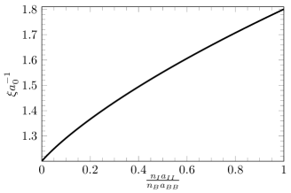
Figure 1: The inverse resonance length $a_{0}^{-1}$ (units of the inverse healing length $\xi$) for bosonic impurities as a function of $n_{I}a_{II}/(n_{0}a_{BB})$, i.e. the ratio of the densities times the ratio of the scattering lengths. The masses of the impurities and the bosons are considered the same, i.e. $m_{B}=m_{I}$ (corresponding to the experimental realization of Ref. Jørgensen et al. (2016)).

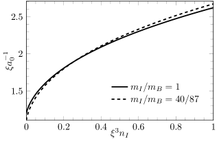
Figure 2: The inverse resonance length $a_{0}^{-1}$ (units of the inverse healing length $\xi$) as a function of the impurity density $n_{I}$ (units of $\xi^{-3}$) for fermionic impurities. The full line is for equal impurity and boson masses, i.e. $m_{B}=m_{I}$, the dashed line corresponds to the mass imbalance for a ${}^{40}\text{K}$ impurity in a ${}^{87}\text{Rb}$ condensate, i.e. $m_{I}/m_{B}=40/87$ (corresponding to the experimental realization of Ref. Hu et al. (2016)).

In Figs. 3 and 4 the polaron energy is presented as a function of the inverse boson-impurity scattering length $a_{IB}^{-1}$. This reveals the well-known resonance behavior with an attractive and a repulsive polaron branch (as also described in Refs. Rath and Schmidt (2013); Jørgensen et al. (2016); Shchadilova et al. (2016) for a single impurity). In Fig. 3 the result for a single impurity is compared with the result in the presence of a Bose-condensed gas of bosonic impurities characterized by the ratio $n_{I}a_{II}/(n_{0}a_{BB})=0.1$. This clearly reveals a shift of the resonance position due to the presence of multiple interacting impurities. In Fig. 4 a similar shift of the resonance is found for the case of non-interacting fermionic impurities characterized by the dimensionless quantity $n_{I}\xi^{3}=0.016$ and with a mass imbalance $m_{I}/m_{B}=40/87$.

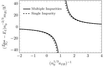
Figure 3: The polaron energy as a function of the inverse boson-impurity scattering length $a_{IB}$ (in units of $n_{0}^{1/3}$) for bosonic impurities in a Bose-Einstein condensate. The dashed line is for a single impurity while the full curve corresponds to a non-zero impurity density characterized by $n_{I}a_{II}/(n_{0}a_{BB})=0.1$. The condensate gas parameter is set to $n_{0}^{1/3}a_{BB}=0.03$ and the impurity and boson masses are the same, i.e. $m_{B}=m_{I}$ (corresponding to the experimental realization presented in Ref. Jørgensen et al. (2016)).

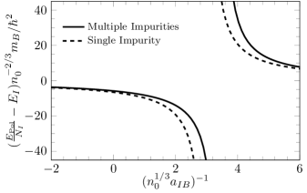
Figure 4: The polaron energy as a function of the inverse boson-impurity scattering length $a_{IB}$ (in units of $n_{0}^{1/3}$) for fermionic impurities in a Bose-Einstein condensate. The dashed line is for a single impurity while the full curve corresponds to a non-zero impurity density characterized by $n_{I}\xi^{3}=0.016$. The condensate gas parameter is set to $n_{0}^{1/3}a_{BB}=0.3$ and the impurity-boson mass imbalance is $m_{I}/m_{B}=40/87$ (corresponding to the experimental realization presented in Ref. Hu et al. (2016)).

In Figs. 5 and 6 the effective mass is presented as a function of the inverse impurity-boson scattering length $a_{IB}^{-1}$ for bosonic and fermionic impurities, respectively. This reveals that the effective mass increases as the resonance is approached. At the resonance the effective mass diverges, signaling the break-down of the polaron quasiparticle picture in this regime, in agreement with the conclusions of Ref. Shchadilova et al. (2016). Similar as for the energy we again observe a clear shift of the resonance due to the many-body nature of the impurities, both for the bosonic and the fermionic impurities.

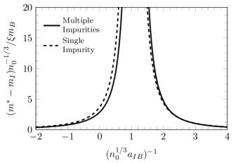
Figure 5: The polaron effective mass as a function of $(n_{0}^{1/3}a_{IB})^{-1}$ for bosonic impurities. The condensate gas parameter is taken $n_{0}^{1/3}a_{BB}=0.03$ and the masses of the impurity and the bosons are considered equal, i.e. $m_{B}=m_{I}$. The dashed line is for a single impurity while the full curve corresponds to an impurity density of $n_{I}a_{II}/(n_{0}a_{BB})=0.1$ (corresponding to the experimental realization presented in Ref. Jørgensen et al. (2016)).

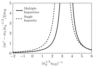
Figure 6: The polaron effective mass as a function of $n_{0}^{1/3}a_{IB}$ for fermionic impurities. The condensate gas parameter is taken $n_{0}^{1/3}a_{BB}=0.3$ and an impurity-boson mass imbalance of $m_{I}/m_{B}=40/87$ is considered. The dashed line is for a single impurity while the full curve corresponds to a finite impurity density characterized by $n_{I}\xi^{3}=0.016$. (corresponding to the experimental realization presented in Ref. Hu et al. (2016)).

V Conclusions and perspectives

We have extended the many-body description for a gas of Fröhlich polarons to interacting Bose polarons, taking into account terms in the Hamiltonian that are beyond the Fröhlich approximation. In order to solve the resulting equations analytically we have introduced an approximation for the anomalous expectation value containing three times the impurity density operator. As for the Fröhlich polaron, the key ingredient that characterizes the impurity gas is the static structure factor. This approximation also allowed us to derive the effective mass of the Bose polarons. These results were applied for the system parameters corresponding to two recent experimental realizations of the Bose polaron Hu et al. (2016); Jørgensen et al. (2016). This reveals a shift of the resonance position with respect to the single polaron result, which is a consequence of the many-body nature of the impurities. Our results also show that in the limit of many impurities the polaronic mass effect disappears. As the resonance is approached the polaron effective mass increases and ultimately diverges which indicates the break-down of our description close to the resonance. A future perspective is about the fate of the Bose polaron in this regime of strong impurity-boson interaction close to the resonance. An extension of the polaronic strong coupling theory, which is well-established for the Fröhlich polaron Lee and Gunn (1992); Kalas and Blume (2006); Cucchietti and Timmermans (2006); Casteels et al. (2011b), to the Bose polaron could shine light on this interesting open question.

Appendix A Anomalous expectation value

In this Appendix we clarify the approximation (6) of the anomalous expectation value

$$\mathcal{I}({\bf{k}},{\bf{q}})=\langle\psi|\hat{\rho}_{{\bf{q}}-{\bf{k}}}\hat{\rho}_{{\bf{k}}}\hat{\rho}_{-{\bf{q}}}|\psi\rangle=\sum\limits_{j,m,n=1}^{N_{I}}\langle\mathrm{e}^{\mathrm{i}{\bf{q}}.(\hat{{\bf{r}}}_{j}-\hat{{\bf{r}}}_{n})}\mathrm{e}^{\mathrm{i}{\bf{k}}.(\hat{{\bf{r}}}_{m}-\hat{{\bf{r}}}_{j})}\rangle.$$ (17)

This expectation value is a special case of the three-point correlation function $\langle\hat{\rho}_{\bf{k_{1}}}\hat{\rho}_{\bf{k_{2}}}\hat{\rho}_{\bf{k_{3}}}\rangle$. The density operators can be expanded around their expectation value $\hat{\rho}_{\bf{k}}\rightarrow\hat{\rho}_{\bf{k}}-\langle\hat{\rho}_{\bf{k}}\rangle,$ which connects the moments to the central moments, as one considers the three-point correlation function as the third moment of the density distribution. Then approximating that the third central moment is zero provides an approximation of the three-point correlation function in terms of one- and two-point correlation functions. Performing the central moment approximation to the two-point correlation function corresponds to the Hartree approximation, which would reduce the three-point correlation function to a product of three expectation values of the density.

We extend this idea to the anomalous expectation value (17) by introducing the structure factor (5) to write down the central moment

$$\mathcal{I}_{\mathrm{central}}({\bf{k}},{\bf{q}})=\sum\limits_{j,m,n=1}^{N_{I}}\left\langle\left(\mathrm{e}^{\mathrm{i}{\bf{q}}.(\hat{{\bf{r}}}_{j}-\hat{{\bf{r}}}_{n})}-\frac{1}{N_{I}}S({\bf{q}})\right)\left(\mathrm{e}^{\mathrm{i}{\bf{k}}.(\hat{{\bf{r}}}_{m}-\hat{{\bf{r}}}_{j})}-\frac{1}{N_{I}}S({\bf{k}})\right)\right\rangle.$$ (18)

The approximation $\mathcal{I}_{\mathrm{central}}\approx 0$ then reduces to

$$\mathcal{I}({\bf{k}},{\bf{q}})\approx N_{I}S({\bf{k}})S({\bf{q}}),$$ (19)

as in Eq. (6). Note that when $\bf{q}\to 0$ ($\bf{k}\to 0$), we get $\mathcal{I}({\bf{k}},0)=N_{I}^{2}S({\bf{k}})$ (and $\mathcal{I}(0,{\bf{q}})=N_{I}^{2}S({\bf{q}})$), such that the central moment approximation is exact in these limits (since $S(0)=N_{I}$). In the expression for the polaronic energy (4) the terms where $\mathcal{I}({\bf{k}},{\bf{q}})$ occurs have to be summed over all $\bf{k},\bf{q}$ after multiplication by a prefactor. As this prefactor is largest when either $\bf{k}$ or $\bf{q}$ are close to zero, the terms where the approximation (19) holds can be expected to provide the dominant contribution.

References

- Landau (1933) L. Landau, Phys. Z. Sowjetunion 3, 664 (1933).
- Fröhlich (1954) H. Fröhlich, Advances in Physics 3, 325 (1954), http://dx.doi.org/10.1080/00018735400101213 .
- Devreese (2010) J. T. Devreese, ArXiv e-prints (2010), arXiv:1012.4576 [cond-mat.other] .
- Lee et al. (1953) T. D. Lee, F. E. Low, and D. Pines, Phys. Rev. 90, 297 (1953).
- Lemmens et al. (1977) L. F. Lemmens, F. Brosens, and J. T. Devreese, physica status solidi (b) 82, 439 (1977).
- Schirotzek et al. (2009) A. Schirotzek, C.-H. Wu, A. Sommer, and M. W. Zwierlein, Phys. Rev. Lett. 102, 230402 (2009).
- Koschorreck et al. (2012) M. Koschorreck, D. Pertot, E. Vogt, B. Fröhlich, M. Feld, and M. Köhl, Nature (London) 485, 619 (2012), arXiv:1203.1009 [cond-mat.quant-gas] .
- Grusdt and Demler (2015) F. Grusdt and E. Demler, ArXiv e-prints (2015), arXiv:1510.04934 [cond-mat.quant-gas] .
- Kalas and Blume (2006) R. M. Kalas and D. Blume, Phys. Rev. A 73, 043608 (2006).
- Cucchietti and Timmermans (2006) F. M. Cucchietti and E. Timmermans, Phys. Rev. Lett. 96, 210401 (2006).
- Tempere et al. (2009) J. Tempere, W. Casteels, M. K. Oberthaler, S. Knoop, E. Timmermans, and J. T. Devreese, Phys. Rev. B 80, 184504 (2009).
- Casteels et al. (2011a) W. Casteels, J. Tempere, and J. T. Devreese, Phys. Rev. A 84, 063612 (2011a).
- Casteels et al. (2013) W. Casteels, J. Tempere, and J. T. Devreese, The European Physical Journal Special Topics 217, 163 (2013).
- Blinova et al. (2013) A. A. Blinova, M. G. Boshier, and E. Timmermans, Phys. Rev. A 88, 053610 (2013).
- Nascimbène et al. (2009) S. Nascimbène, N. Navon, K. J. Jiang, L. Tarruell, M. Teichmann, J. McKeever, F. Chevy, and C. Salomon, Phys. Rev. Lett. 103, 170402 (2009).
- Heinze et al. (2011) J. Heinze, S. Götze, J. S. Krauser, B. Hundt, N. Fläschner, D.-S. Lühmann, C. Becker, and K. Sengstock, Phys. Rev. Lett. 107, 135303 (2011).
- Will et al. (2011) S. Will, T. Best, S. Braun, U. Schneider, and I. Bloch, Phys. Rev. Lett. 106, 115305 (2011).
- Catani et al. (2012) J. Catani, G. Lamporesi, D. Naik, M. Gring, M. Inguscio, F. Minardi, A. Kantian, and T. Giamarchi, Phys. Rev. A 85, 023623 (2012).
- Hohmann et al. (2015) M. Hohmann, F. Kindermann, B. Gänger, T. Lausch, D. Mayer, F. Schmidt, and A. Widera, EPJ Quantum Technology 2, 23 (2015).
- Rentrop et al. (2016) T. Rentrop, A. Trautmann, F. A. Olivares, F. Jendrzejewski, A. Komnik, and M. K. Oberthaler, Physical Review X 6, 041041 (2016).
- Hu et al. (2016) M.-G. Hu, M. J. Van de Graaff, D. Kedar, J. P. Corson, E. A. Cornell, and D. S. Jin, Phys. Rev. Lett. 117, 055301 (2016).
- Jørgensen et al. (2016) N. B. Jørgensen, L. Wacker, K. T. Skalmstang, M. M. Parish, J. Levinsen, R. S. Christensen, G. M. Bruun, and J. J. Arlt, Phys. Rev. Lett. 117, 055302 (2016).
- Levinsen et al. (2015) J. Levinsen, M. M. Parish, and G. M. Bruun, Phys. Rev. Lett. 115, 125302 (2015).
- Shchadilova et al. (2016) Y. E. Shchadilova, R. Schmidt, F. Grusdt, and E. Demler, Phys. Rev. Lett. 117, 113002 (2016).
- Grusdt et al. (2017) F. Grusdt, G. E. Astrakharchik, and E. Demler, New Journal of Physics 19, 103035 (2017).
- Camacho-Guardian and Bruun (2018) A. Camacho-Guardian and G. M. Bruun, Phys. Rev. X 8, 031042 (2018).
- Nakano and Yabu (2016) E. Nakano and H. Yabu, Phys. Rev. B 93, 205144 (2016).
- Rath and Schmidt (2013) S. P. Rath and R. Schmidt, Phys. Rev. A 88, 053632 (2013).
- Lee and Gunn (1992) D. K. K. Lee and J. M. F. Gunn, Phys. Rev. B 46, 301 (1992).
- Casteels et al. (2011b) W. Casteels, T. Van Cauteren, J. Tempere, and J. T. Devreese, Laser Physics 21, 1480 (2011b).