Investigating the nonequilibrium aspects of long-range Potts model: refinement of critical temperatures and raw exponents

Abstract

In this work, we analyse the $q-$state Potts model with long-range interactions through nonequilibrium scaling relations commonly used when studying short-range systems. We determine the critical temperature via an optimization method for short-time Monte Carlo simulations. The study takes into consideration two different boundary conditions and three different values of range parameters of the couplings. We also present estimates of some critical exponents, named as raw exponents for systems with long-range interactions, which confirm the non-universal character of the model. Finally, we provide some preliminary results addressing the relations between the raw exponents and the exponents obtained for systems with short-range interactions. The results assert that the methods employed in this work are suitable to study the considered model and can easily be adapted to other systems with long-range interactions.

In a famous paper published in 1969, Freeman J. Dyson [1] showed the existence of phase transition in a one-dimensional Ising system with long-range interactions whose Hamiltonian is given by

$$\mathcal{H}=-\sum_{i<j}J_{ij}s_{i}s_{j}$$ (1)

where $J_{ij}=J(\left|i-j\right|)$ is the coupling constant and $s_{i}=\pm 1$. For that system, two conditions must be fulfilled:

$$\begin{array}[]{lll}\text{(1)}&I_{1}=\sum_{n=1}^{\infty}J(n)<\infty&\\ &&\\ \text{(2)}&I_{2}=\sum_{n=1}^{\infty}\frac{\ln(\ln n)}{n^{3}J(n)}<\infty&\end{array}$$

Such linear interacting spin systems, obviously, do not affect the Landau argument which refers to local interacting spins. An important class of long-range (LR) couplings that satisfies such conditions is that of algebraic decay:

$$J(n)=\frac{C}{n^{(1+\sigma)}}\$$ (2)

with $0<\sigma<1$, since $\ I_{1}<\int_{1}^{\infty}\frac{dx}{x^{1+\sigma}}=\frac{1}{\sigma}$ and

$$\begin{array}[]{lll}I_{2}&\leq&\frac{1}{C}\sum_{n=1}^{\infty}\frac{\ln n}{n^{2-\sigma}}\\ &&\\ &\leq&\frac{1}{C}\int_{1}^{\infty}\frac{\ln x}{x^{2-\sigma}}dx<\infty\text{.}\end{array}$$ (3)

Here, $\sigma$ is the range parameter of the coupling. Thus, we certainly expect a phase transition for such $\sigma$-values. This particular and sufficient condition for the existence of a critical phenomena was conjectured by Kac and Thompson [2] in the same year of Dyson’s publication.

The Hamiltonian of the one-dimensional $q-$state Potts model with long-range interactions can be written as a generalization of the LR Ising model given by Eq. (1) along with the coupling constant presented in Eq. (2). It is given by

$$\beta\mathcal{H}_{\text{Potts}}=-K\sum_{i<j}\ \frac{\delta_{s_{i},s_{j}}}{\left|i-j\right|^{1+\sigma}}$$ (4)

where $\beta=(k_{B}T)^{-1}$ with $k_{B}$ being the Boltzmann constant and $T$ the temperature of the system, $K=\beta J$ is the coupling coefficient, $i,j=1,...,L$, and $L$ is the chain length. At equilibrium, one can calculate the $k$-th moments of magnetization:

$$\left\langle M^{k}\right\rangle=\frac{1}{L^{k}(q-1)^{k}}\left\langle\left(\sum_{i=1}^{L}(q\delta_{s_{i},1}-1)\right)^{k}\right\rangle$$ (5)

where $\left\langle(\cdot)\right\rangle=\frac{1}{Z}\sum_{\left\{s_{i}\right\}}(\cdot)\exp\left[-\mathcal{H}_{\text{Potts}}\right]$, and $Z=\sum_{\left\{s_{i}\right\}}\exp\left[-\mathcal{H}_{\text{Potts}}\right]$.

Exactly as reported by Dyson, here it is expected the existence of a critical temperature $T_{c}$ (or similarly, $K_{c}$). Hence, the susceptibility $\chi=L\left(\left\langle M^{2}\right\rangle-\left\langle M\right\rangle^{2}\right)$, for instance, must behave as $\chi\sim\frac{1}{(T-T_{c})}$ at the critical point also for $q>2$ as expected for spin systems with short-range (SR) interactions.

In 1989, Glumac and Uzelac [3] obtained estimates for $K_{c}$ by performing a study for the LR Ising model through a method that scales the range of interactions. The same authors extended such estimates in 1993 for the LR Potts model by making use of the transfer matrix method [4]. Although they presented important contributions to the field, we believe that more attention should be given in systems with LR interactions by employing new methods and approaches in order to obtain refined estimates of the critical parameters.

Monte Carlo (MC) equilibrium methods can be an efficient approach to validate such estimates of $T_{c}\ (K_{c})$, but in LR systems they are very expensive. Thus, an interesting alternative to achieve this goal is through nonequilibrium MC methods. In this context, we can highlight the short-time dynamics theory deduced and developed by a set of authors from analytical [6] and numerical [7] points of view. This approach was developed in the context of model A, according to the definition of Halperin, Hohenberg, and Ma [8]. This definition considers the relaxational dynamics of a non-conserved order parameter described by the solution of the Langevin equation for the Landau-Ginzburg-Wilson Hamiltonian. Although it has been extensively investigated for models with SR interactions, systems with LR interactions have not being subject of study. However, an important aspect of these interactions is that they can modify the critical equilibrium properties of the system in consideration.

This method, known as short-time MC simulations, takes into consideration different time series of the order parameter (the magnetization for most of the spin models) and its moments. Each time series starts with a fixed initial magnetization $m_{0}$ and then, the system is quenched from high temperatures to the critical one. The time evolution of the $k-$th moment of the magnetization obeys the following general scaling relation:

$$\overline{M^{k}}(t,\tau,L,m_{0})=b^{-\frac{k\beta}{\nu}}\overline{M^{k}}(b^{-z}t,b^{\frac{1}{\nu}}\tau,b^{-1}L,b^{x_{0}}m_{0}).$$ (6)

Here, $t$ is the time evolution, $b$ is an arbitrary spatial rescaling factor, $\tau=\left(T-T_{c}\right)/T_{c}$ is the reduced temperature and $L$ is the size of the one-dimensional lattice. This evolution is governed by a new dynamic critical exponent $\theta$ which is independent of the well known static critical exponents, e.g. $\beta$ and $\nu$, and the dynamic exponent $z$. This new exponent characterizes the so-called critical initial slip, the anomalous behavior of the magnetization when the system is quenched to the critical temperature $T_{c}$. In addition, a new critical exponent $x_{0}$ which represents the anomalous dimension of the initial magnetization $m_{0}$, is introduced to describe the dependence of the scaling behavior on the initial conditions. This exponent is related to $\theta$ as $x_{0}=\theta z+\beta/\nu$.

Unlike $\left\langle O\right\rangle$, the quantity $\overline{O}$ describes an average over different random evolutions and initial conditions of the system. Here, $O$ is a general symbol which means the magnetization or their superior moments calculated through MC simulations as an average over all $L$ spins and over different $N_{run}$ runs (the number of different time evolutions):

$$\overline{O}(t)=\frac{1}{N_{run}\ L}\sum\limits_{r=1}^{N_{run}}\sum\limits_{i=1}^{L}O_{i,r}(t),$$ (7)

where the index $r=1,...,N_{run}$ denotes the corresponding run of each simulation.

Several authors have performed short-time MC simulations in order to obtain the following two dynamic critical exponents: the exponent $\theta$, which governs the critical initial slip of the magnetization $\overline{M}\sim m_{0}t^{\theta}$ and the exponent $z$ which characterizes the time correlation in equilibrium (for two good reviews see Albano et al. [9] and B. Zheng [7]). The exponent $z$, for instance, can be obtained considering the second moment of the magnetization, which is written as

$$\overline{M_{m_{0}=0}^{2}}=\frac{1}{L^{2d}}\sum\limits_{i=1}^{L^{d}}\overline{\sigma_{i}^{2}}+\frac{1}{L^{2d}}\sum\limits_{i\neq j}^{L^{d}}\overline{\sigma_{i}\sigma_{j}}\approx L^{-d}$$

for a fixed $t$. By taking into account $k=2$ in Eq. (6) with $b=t^{1/z}$ and considering that the spin-spin correlation $\overline{\sigma_{i}\sigma_{j}}$ is negligible for $m_{0}=0$ (with spins randomly distributed over the lattice), we obtain the following power law for the second moment of the magnetization at $T=T_{c}$:

$$\begin{array}[]{lll}\overline{M_{m_{0}=0}^{2}}(t,L)&\approx&t^{\frac{-2\beta}{\nu z}}\overline{M_{m_{0}=0}^{2}}(1,t^{-1/z}L)\\ &&\\ &=&t^{\frac{-2\beta}{\nu z}}(t^{-1/z}L)^{-d}\\ &&\\ &\sim&t^{(d-\frac{2\beta}{\nu})/z}\text{. }\end{array}$$ (8)

Recently, Uzelac et. al [5] used the critical temperatures obtained in their previous works [4, 3] to perform short-time MC simulations in order to present a preliminary study of the dynamic critical exponents $\theta$ and $z$ of the Potts model with LR interactions described by the Hamiltonian given by Eq. (4) for the cases $q=2$ and 3.

Although the Ref. [5] shows a lot of interesting things that motivated this current work, in our opinion, the computing of critical exponents by simply transposing the finite-size scaling of the short-time dynamics used for SR systems deserves a lot of further investigations, since Eq. (6) should not work for LR systems, and to the best of our knowledge, there is nothing in literature suggesting this.

This undoubtedly is not clear as reported by other authors as Chen et. al [10]. That work which has L. Schulke, one of the precursors in the study of short-time dynamics for SR systems, as one of the authors, proposes a study of the short-time critical behavior of the $d-$dimensional Ginzburg-Landau model with LR interactions. The authors include an LR term in the Landau-Ginzburg-Wilson Hamiltonian for the time evolution described by the Langevin equation in order to obtain the short-time scaling relations similar to that given by Eq. (6). The exponent $\theta$ which characterizes the critical initial slip of the magnetization is an independent exponent explored in that work. However, they did not point out a way to explore other power laws to obtain estimates for other exponents from those LR systems.

Moreover, an important question is if we can use nonequilibrium methods, in a more fundamental point of view, to estimate critical temperatures of LR interaction models and not only their critical exponents, since there is not a consensus about the precision of these estimates from previous results presented in literature, to the best of our knowledge. So, in this work we aim to present the estimates of the critical temperatures of the Potts model with long-range interactions through nonequilibrium methods based on an optimization method in the context of time dependent Monte Carlo simulations proposed in Ref. [11].

In order to answer that question, we look into a simpler power law (for the initial condition $m_{0}=1$) and keep the traditional order parameter of the Potts model and their superior moments defined by Eq. (5). These ways of analyzing the system were not considered in Ref. [5] and, as we will show below, they are important to help shed light on this topic.

Particularly in the case of $(m_{0}=1)$, the system loses the dependence on initial conditions and the first moment of the magnetization must decay, at criticality, as

$$\overline{M_{m_{0}=1}}(t)\sim t^{-\delta}$$ (9)

where $\delta$, which is our first raw exponent for LR systems, is given by $\delta=\frac{\beta}{\nu z}$ for models with SR interactions. So, we will simply denote the exponent by $\delta=\delta_{LR}$ whereas, to the best of our knowledge, the literature does not show any information about similarities between short- and long-range exponents.

From now on, we adopt a cautious prescription by considering that the power laws must exist at the criticality and their exponents are given as raw exponents. With this assumption, the power law given by Eq. (8) must be redefined since we do not expect the existence of critical points for one-dimensional SR systems. Therefore, for LR systems starting with $m_{0}=0$, we appropriately consider $\overline{M_{m_{0}=0}^{2}}(t)\sim t^{\xi_{LR}}$.

Regarding this letter, our initial intent was to study the localization of the critical points of the $q-$state Potts Model with LR interactions via time-dependent MC simulations by estimating the best $K_{c}$ for a given $q$ through a technique based on a statistical concept known as coefficient of determination. In this approach, we set as input parameter the coupling coefficient $K^{(\min)}$ (initial value) and run simulations for different values of $K$ according to a resolution $\Delta K$. In order to show the robustness of the method, we carried out simulations for $q=2$, $3$, and $4$. We also change the range parameter $\sigma$, considering $\sigma=0.7$, $0.8$, and $0.9$. With all these analysis in hand, we are just one step to obtain the critical exponents and explore the universality of the system. So, we include these estimates as a second part of our study, at the end of this work. The simulations were carried out by considering free boundary conditions (FBC). However, we also perform some simulations with periodic boundary conditions (PBC), in order to compare the results. The latter boundary condition was considered in Ref. [12] for the study of the LR Potts model through MC simulations at equilibrium. For PBC, the distance between two sites is $d(i,j)=\min(j-i,i+L-j)$, with $i<j$, such that $\max_{i,j}d(i,j)=L/2$.

Since at criticality it is expected that the order parameter obeys the power law behavior given by Eq. (9), we performed MC simulations for each value $K=K^{(\min)}+i\Delta K$, with $i=1,...,n$, where $n=\left\lfloor(K^{(\max)}-K^{(\min)})/\Delta K\right\rfloor$, and calculated the coefficient of determination $r$, which is given by

$$r=\frac{\sum\limits_{t=t_{\min}}^{t_{\max}}(\overline{\overline{\ln\overline{M}}}-a-b\ln t)^{2}}{\sum\limits_{t=t_{\min}}^{t_{\max}}(\overline{\overline{\ln\overline{M}}}-\ln\langle M\rangle(t))^{2}},$$ (10)

with $\overline{\overline{\ln\overline{M}}}=\frac{1}{(t_{\max}-t_{\min})}\sum\nolimits_{t=t_{\min}}^{t_{\max}}\ln\overline{M}(t)$. The critical value $K_{c}$ corresponds to $K^{(opt)}=\arg\max_{K\in[K^{(\min)},K^{(\max)}]}\{r\}$ and, $a$ and $b$ are, respectively, the slope and intercept obtained from the linearization. Here, $t_{\min}$ is the number of discarded MC steps and $t_{\max}$ the maximum number of MC steps used in our simulations.

The coefficient $r$ extends from 0 to 1 and has a very simple explanation: it measures the ratio: (expected variation)/(total variation). So, the bigger the $r$, the better the linear fit in log-scale, and therefore, the better the power law which corresponds to the critical parameter excepted for an order of error $\Delta K$.

Here, we use a very simple procedure: we consider $\Delta K=0.01$, $N_{run}=2000$ runs, $L=3000$ sites, and choose (with no previous information) $K^{(\min)}$ and $K^{(\max)}$ for each value of $q$ and $\sigma$. By varying $K$, we are able to determine its optimal value, $K^{(opt)}$, which is considered the critical point for the set $(q,\ \sigma)$. In our simulations, we used a total number of $N_{MC}=60$ MC steps (where $t_{\max}\leq N_{MC}$), which is bigger than that used, for instance, in Ref. [5] ($N_{MC}=40$ MC steps). In this approach, we obtain curves of $r$ as function of $K$ by discarding $t_{\min}=5$ MC steps and varying $t_{\max}=20$, 40, and 60, as shown in Fig. 1.

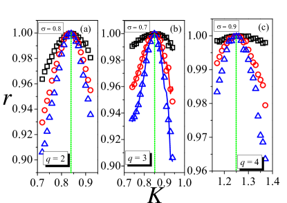
Figure 1: Coefficient of determination as function of $K$. We show three examples: $q=2,\ 3$, and 4, respectively, for three coupling parameters $\sigma=0.8$, $0.7$ and $0.9$. Squares, balls, and triangles correspond to different values of $t_{\max}$ used to calculate the coefficient of determination: 20, 40, and 60, respectively. The continuous curves in plot (b) correspond to the results with periodic boundary conditions.

In this figure, we show three examples of optimizing curves $r\times K$, for $q=2,\ 3$, and 4, respectively, for three coupling-parameters $\sigma=0.8,\ 0.7$, and $0.9$, for FBC. Figure 1 (b) also presents our estimates for PBC (continuous lines) and, as can be seen, the results for both boundary conditions are in excellent agreement. So, we can assert that both FBC and PBC produce good estimates and, therefore, in the remaining of this work, we consider only FBC to obtain our results.

In order to obtain the final estimates of $K_{c}$, instead of considering a smaller $\Delta K$ in the region where $r\simeq 1$ to refine our results, we perform quadratic curve-fittings on $r\times K$ and consider the summit of each curve as our best estimate. For a comparison of our results with those ones shown in Ref. [4] (based on transfer matrix method), we decided to present our estimates with four decimal digits. It is important to notice that sometimes the authors present the results with two, three, or even four significant digits. We arbitrarily use their estimates with four significant digits by default.

Figure 2 shows curves of the time evolution of the order parameter for the best critical point $K_{c}$ obtained in this work along with the results found in Ref. [4].

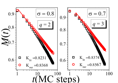
Figure 2: Decay of magnetization using our best estimates for $K_{c}$ and those ones found in Ref. [4]. Our results clearly show better power law behaviors as expected for magnetization at the critical point when $m_{0}=1$, according to Eq. (9).

As can be seen, our results show a notorious visual improvement when compared with the estimates obtained through equilibrium methods. Although Fig. 2 showed only two cases, the improvement in results occurs for all set of parameters studied in this work, confirming the robustness of the methods employed in this work. Our best estimates are presented in the columns two, four, and six of Table 1 and the columns three, five, and seven show the values obtained from Ref. [4].

$K$	$\sigma=0.7$		$\sigma=0.8$		$\sigma=0.9$
	This work	Ref. [4]	This work	Ref. [4]	This work	Ref. [4]
$q=2$	$0.7043$	0.6833	$0.8368$	0.8231	$0.9934$	0.9973
$q=3$	$0.8567$	0.8374	$0.986\,4$	0.9774	$1.1402$	1.1440
$q=4$	$0.957\,6$	0.9540	$1.\,\allowbreak 095\,9$	1.0930	$1.2524$	1.2550

Table 1: Critical coupling coefficients obtained with the method based on the coefficient of determination for the $q-$state LR Potts model for $q=2$, 3, and 4. We studied these models considering three different range parameters: $\sigma=0.7$, 0.8, and 0.9. The results are compared with the estimates found in Ref. [4].

With the results of the critical parameters in hand, we decided to look into the behavior of the power laws related to the magnetization or other more complex quantities at criticality, as it is traditionally done in the study of SR systems via time-dependent MC simulations.

For those systems, we showed in Ref. [13] that combining simulations with different initial conditions, one produces a cumulant $F_{2}(t)=$ $\overline{M_{m_{0}=0}^{2}}(t)/\overline{M_{m_{0}=1}}^{2}(t)$ which, in turn, behaves as $F_{2}(t)\sim t^{d/z}$, where $d$ is the dimension of the system. So, this cumulant supplies the dynamic critical exponent $z$ without the need of static exponents previously calculated by other methods or even conjectured in literature. In this work, we also conjecture that, for LR systems, a similar behavior is expected, i.e.,

$$F_{2}(t)\sim t^{\gamma}.$$ (11)

Here, we would like to reinforce that we do not intent to conjecture any dependence of the exponents obtained for LR systems with those of SR ones. For this reason, we present the $\gamma$ as a raw exponent.

In SR models, the static critical exponent $\nu$ can be obtained if the exponent $z$ is estimated in advance, as for instance, through the cumulant $F_{2}$. By using a power law which considers simulations of the order parameter slightly off the critical temperature $T_{c}\pm\delta$, with $\delta<<1$, the derivative $D(t)=\frac{\partial}{\partial T}\ln\overline{M}_{m_{0}}(t,T)|_{T=T_{c}}$ can be numerically estimated by $D(t)=\frac{1}{2\delta}\ln\frac{\overline{M}_{m_{0}}(t,T_{c}+\delta)}{\overline{M}_{m_{0}}(t,T_{c}-\delta)}$. For SR systems, this function behaves as $D(t)\sim t^{1/\nu z}$ and, for LR systems, we simply set it as

$$D(t)\sim t^{\xi}.$$ (12)

So, from now on we focus our attention on the study of the raw exponents $\delta$, $\gamma$, and $\xi$, given respectively by the Eqs. (9), (11), and (12). In Fig. 3 we show the power law behaviors expected for these equations when considering $q=2,\ 3,$ and $4$, and for three values of the range parameter: $\sigma=0.7$, $0.8$, and $0.9$. These curves were obtained by carrying out simulations of the model at the best critical parameters obtained above and showed in Table 1.

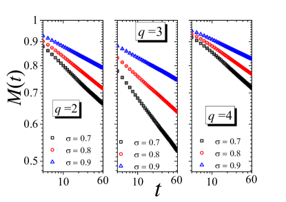
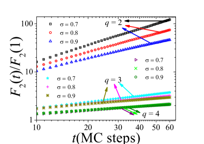
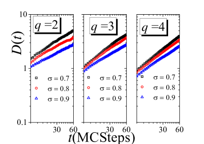
Figure 3: Power law behavior of the Eqs. (9), (11), and (12) for $q=2,\ 3,$ and $4$ and $\sigma=0.7,\ 0.8$, and 0.9.

From the slope of these power laws (in log scale), we obtained the exponents $\delta$, $\gamma$, and $\xi$, and their respective error bars which were estimated from 5 independent time series averaged over $N_{run}=2000$ runs. The columns five, nine, and thirteen of Table 2 correspond to the critical exponents of the standard two-dimensional $q-$state Potts model with short-range interactions from Refs. [6, 13, 14].

	${\tiny q=2}$				${\tiny q=3}$				${\tiny q=4}$
${\tiny\sigma}$	${\tiny 0.7}$	${\tiny 0.8}$	${\tiny 0.9}$	${\tiny d=2}$	${\tiny 0.7}$	${\tiny 0.8}$	${\tiny 0.9}$	${\tiny d=2}$	${\tiny 0.7}$	${\tiny 0.8}$	${\tiny 0.9}$	${\tiny d=2}$
${\tiny\delta}$	0.1433(4)	0.0979(3)	0.0619(4)	0.0580	0.1017(7)	0.0881(2)	0.0589(1)	0.0607	0.0974(3)	0.0776(1)	0.0549(1)	0.0546
${\tiny\gamma}$	1.100(4)	0.958(4)	0.808(5)	0.928	0.417(1)	0.339(2)	0.288(2)	0.911	0.280(1)	0.263(1)	0.231(2)	0.873
${\tiny\xi}$	0.65(2)	0.58(2)	0.55(2)	0.46	0.72(1)	0.68(1)	0.59(1)	0.55	0.80(1)	0.76(1)	0.68(1)	0.66

Table 2: Critical Exponents $\delta$, $\gamma$, and $\xi$, for the $q-$state Potts model with long-range interactions. There is a tendency of the exponents to decrease for increasing values of $\sigma$ and $q$, except for the exponent $\xi$ which increases when $q$ enlarges.

As shown in Table 2, the exponents $\delta$ and $\gamma$ decrease as $q$ enlarges. The same does not occur for $\xi$ which increases for higher values of $q$. However, all exponents decrease when the interaction exponent $\sigma$ increases, for all values of $q$. The columns named with $d=2$ present estimates of the exponents calculated for the two-dimensional SR (each spin on the lattice interacts only with its nearest neighbors) Potts model (as it is well known, there is no phase transition for this model when $d=1$). In this case, we consider $\beta$, $\nu$, and $z$ obtained in Refs. [13, 14, 15]. When comparing our results with the estimates from literature, we observe an interesting finding: the exponents $\delta$ and $\xi$ approach to the result for the SR regime as $\sigma$ increases. The most similar case is for $q=4$ since $\delta_{LR}(\sigma=0.9)=0.0549(1)$ and $\delta_{SR}=0.0546$, and $\xi_{LR}(\sigma=0.9)=0.68(1)$ and $\xi_{SR}=0.66$. For a more reliable comparison, we use the same number of significant digits for the two approaches. We present the SR measures without uncertainty bars since the only source of error bars is from the exponent $z$ since $\beta$ and $\nu$ are exact measures. In addition, this variation of the exponents for a given $q$ when $\sigma$ varies confirms that the LR Potts model exhibits a non-universal behavior.

To explore the only method that should supply the exponent $z$ independently, we can carry out a very preliminary study for the system with LR interactions by adopting that $\gamma=\frac{d}{z}$ where $d=1$ (which does not hold when thinking of the SR case). So, by performing this extrapolation for $q=2$, we obtain $z=0.909(4)$, $1.044(4)$, and $1.238(6)$ for $\sigma=0.7$, $0.8$, and $0.9$, respectively. In Ref. [5], the authors used an alternative order parameter given by $M_{x}=L^{-1}q/(q-1)\max_{\alpha}\sum_{i}\left(\delta_{s_{i},\alpha}-1/q\right)$, denoted by them as absolute value of the magnetization, and also considered a correspondence between this parameter and the quantity $\sqrt{\overline{M_{m_{0}=0}^{2}}}$ deduced according to the scaling relation valid for SR systems (Eq. 8). In that case, they argued that $M_{x}$ behaves as $t^{(d/2-\frac{\beta}{\nu})/z}$ and then considered that $\beta/\nu=\frac{1-\sigma}{2}$ following Ref. [16]. They found $z=0.81(1)$, $0.96(4)$ and $1.18(4)$ for $\sigma=0.7$, $0.8$, and $0.9$, respectively. Although their estimates are similar to our results, there are some factors which may explain the differences found: 1) We have refined the critical temperature using short-time Monte Carlo simulations. This value is used as input in the study of critical exponents and is, therefore, very important to obtain reliable estimates; 2) We are using a different order parameter and our method does not use other exponents as input parameters to obtain the exponent $z$, i.e., by using the cumulant $F_{2}(t)$, the exponent $z$ is obtained independently.

In our point of view, there are also some issues which must be considered here:

1. The power law for $M_{x}$ used in Ref. [5] takes into consideration only a conjecture and, in addition, some correspondences deserve much more attention when adapted from SR systems to LR ones. To the best of our knowledge, the set of static and dynamic critical exponents presented in the power-laws for systems with SR interactions should not hold for systems with LR interactions;

2. The authors used $\beta/\nu=(1-\sigma)/2$ from Ref. [16] as input parameter to obtain the exponent $z$. After a double check, the Ref. [16] presents as estimate, the exponent $\eta=2-\sigma$. Thus, by considering that $2\beta/\nu=\eta$ (which is valid only to the two-dimensional SR Potts model), we conclude that $\beta/\nu$ is equal to $1-\sigma/2$ instead of $(1-\sigma)/2$ as used by the authors in Ref. [5] to obtain $z$ through $M_{x}$. Therefore, we think that the relation used by them was probably obtained otherwise and, as pointed out above, we think that it is not valid for LR systems.

3. Finally, if we decided to use the Eq. (9) with $\delta=\beta/(\nu z)$ and consider both prescriptions for $\beta/\nu$ addressed above to obtain the exponent $z$, we would find estimates completely different from those presented in Ref. [5].

It is important to consider a final comment and some comparisons of our results with those found in literature. The only case which can be compared with our results in Ref. [12] is for $q=3$ and $\sigma=0.7$. Let us conjecture that it is possible to relate the well known critical exponents of SR systems with the raw exponents. In addition, let us suppose that the exponent $z$ does not appear in the relations for $\delta$ and $\xi$. So, if the raw exponents are given by $\delta\rightarrow\delta_{LR}=\frac{\beta}{\nu}$ and $\xi\rightarrow\xi_{LR}=\frac{1}{\nu}$, what do we obtain? From our results and these relations, we could estimate $\beta$ and $\nu$ independently and compare them with results available in the literature. Therefore, we performed MC simulations to obtain $\delta_{LR}$, $\gamma_{LR}$, and $\xi_{LR}$ with both FBC and PBC. The results for both boundary conditions are in good agreement with each other exactly as ocurred for the critical parameters presented in Table 2. For PBC, we find $\delta_{LR}=0.102(1)$, $\gamma_{LR}=0.419(1)$, and $\xi_{LR}=0.69(1)$ which lead to $\beta=\delta_{LR}/\xi_{LR}=0.148(3)$ and $\nu=1/\xi_{LR}=1.45(2)$. These results are surprisingly in absolute agreement with the estimates obtained in Ref. [12] through the Ferrenberg-Swendsen method [17]: $\beta=0.15(1)$ and $\nu=1.46(1)$.

It is important to observe that $\beta/\nu=0.102(1)$ does not agree with the conjecture used by [5] which, for $\sigma=0.7$ is $\beta/\nu=(1-\sigma)/2=0.15$. Actually, we think that the conjecture must be true for $q=2$ but not for $q=3$. Let us test this statement by using the values of Table 2, this time for $q=2$. According to our hypothesis that reformulates the exponent to $\delta_{LR}=\beta/\nu$, we obtain $\beta/\nu\approx 0.143$ for $\sigma=0.7$, $\beta/\nu\approx 0.098$, for $\sigma=0.8$, and $\beta/\nu=0.062$ when $\sigma=0.9$. If we consider $\beta/\nu=(1-\sigma)/2$, we find, $\beta/\nu=0.15$, $0.10$, and $0.05$ for $\sigma=0.7$, 0.8, and 0.9, respectively, which are in fair agreement with our estimates. This shows that other points deserve a lot of future investigations and the role of $z$ in the raw exponents must be better explored.

In this letter, we presented a useful, suitable, and fast method which has been successfully used to study systems with short-range interactions, and now, has proved to be equally efficient when locating critical points of the $q-$state Potts model with long-range interactions. This approach, which can easily be extended to other systems with long-range interactions, allowed us to obtain the critical temperatures for $q=2$, 3, and 4, and for $\sigma=0.7$, 0.8, and 0.9. With these critical parameters in hand, we carried out short-time Monte Carlo simulations to estimate the exponents $\delta$, $\gamma$, and $\xi$, which we call raw exponents. They are related, respectively, to the power law behaviors of the magnetization $M(t)$, $F(t)=M^{2}(t)/[M(t)]^{2}$ when considering different initial conditions, and $D(t)=\frac{\partial}{\partial T}\ln M(t,T)|_{T=T_{c}}$. Our results showed that, for a given $q$, all three raw exponents studied in this work depend strongly on $\sigma$. This continuous dependence of the critical exponents on the range parameter $\sigma$ shows that the $q-$state Potts model with long-range interactions exhibits non-universal behavior.

Acknowledgements – R. da Silva thanks CNPq for financial support under grant number: 310017/2015-7

References

- [1] F. Dyson, Conmun. Math. Phys. 12, 91–107 (1969)
- [2] M. Kac, C. J. Thompson, J. Math. Phys. 10, 1373 (1969)
- [3] Z. Glumac and K. Uzelac J. Phys. A 22 4439-4452 (1989)
- [4] Z. Glumac and K. Uzelac J. Phys. A 26 5267-5278 (1993)
- [5] K. Uzelac, Z. Glumac, O. Barisic, Eur. Phys. J. B 63, 101 (2008)
- [6] H.K. Janssen, B. Schaub, and B. Schmittmann, Z. Phys. B: Condens. Matter 73, 539 (1989);
- [7] B. Zheng, Int. J. Mod. Phys. B, 12, 1419 (1998); D.A. Huse, Phys. Rev. B 40, 304 (1989)
- [8] B. I. Halperin, P. C. Hohenberg, S-K. Ma, Phys. Rev. B 10, 139 (1974); P. C. Hohenberg, B. I. Halperin, Rev. Mod. Phys. 49, 435 (1977)
- [9] E. V. Albano, M. A. Bab, G. Baglietto, R. A. Borzi, T. S. Grigera, E. S. Loscar, D. E. Rodriguez, M. L. R. Puzzo, G. P. Saracco, Rep. Prog. Phys. 74, 026501 (2011)
- [10] Y. Chen, S.H. Guo, Z.B. Li, S. Marculescu, L. Schülke, Eur. Phys. J. B 18, 289-296 (2000)
- [11] R. da Silva, J.R. Drugowich de Felício, and A.S. Martinez, Phys. Rev. E 85, 066707 (2012)
- [12] E. Bayong, H. T. Diep, V. Dotsenko, Phys. Rev. Lett. 83, 14 (1999)
- [13] R. da Silva, N.A. Alves, and J.R. Drugowich de Felício, Phys. Lett. A 298, 325 (2002)
- [14] F. Y. Wu, Rev. Mod. Phys., 54, 235 (1982)
- [15] R. da Silva, J.R. Drugowich de Felício, Phys. Lett. A 333, 277 (2004)
- [16] E. Brézin, J. Zinn-Justin, J.C. Le Guillou, J. Phys. A 9, L119 (1976)
- [17] A. M. Ferrenberg and R. H. Swendsen, Phys. Rev. Lett. 61, 2635 (1988)