An ensemble based on a bi-objective evolutionary spectral algorithm for graph clustering
Abstract
Graph clustering is a challenging pattern recognition problem whose goal is to identify vertex partitions with high intra-group connectivity. This paper investigates a bi-objective problem that maximizes the number of intra-cluster edges of a graph and minimizes the expected number of inter-cluster edges in a random graph with the same degree sequence as the original one. The difference between the two investigated objectives is the definition of the well-known measure of graph clustering quality: the modularity. We introduce a spectral decomposition hybridized with an evolutionary heuristic, called MOSpecG, to approach this bi-objective problem and an ensemble strategy to consolidate the solutions found by MOSpecG into a final robust partition. The results of computational experiments with real and artificial LFR networks demonstrated a significant improvement in the results and performance of the introduced method in regard to another bi-objective algorithm found in the literature. The crossover operator based on the geometric interpretation of the modularity maximization problem to match the communities of a pair of individuals was of utmost importance for the good performance of MOSpecG. Hybridizing spectral graph theory and intelligent systems allowed us to define significantly high-quality community structures.
keywords:
Graph clustering , Community detection , Evolutionary heuristic , Multi-objective optimization , Modularity maximization , Spectral decomposition1 Introduction
The majority of graphs that describe real networks, such as social and metabolic networks (Zachary, 1977; Lancichinetti et al., 2011), are characterized by vertex partitions with high intra-cluster connectivity (Girvan & Newman, 2002). The graph clustering problem, also known as community detection problem, aims at finding such partitions. Ferrara et al. (2014), for example, developed an expert system to detect communities in mobile phone networks formed by interactions of criminals to possibly identify criminal organizations. Larsson & Moe (2012) and Golbeck et al. (2010) applied community detection algorithms to Twitter data to classify the users’ political leaning. In practice, this type of information usually benefits political campaigners.
The formal definition of a graph clustering problem leans towards the criterion to assess the partitioning quality. Examples of optimization criteria to finding graph clusterings are the maximization of modularity (Newman & Girvan, 2004), the map equation minimization (Rosvall & Bergstrom, 2008) and the maximization of the statistical significance of communities according to the measure introduced by Lancichinetti et al. (2011). In particular, the map equation measure is based on the observation on the duality between graph clustering problems and the data compression problem described by the minimization of the path length of a random walker. The Infomap algorithm was then proposed to detect communities that minimize the map equation. Lancichinetti et al. (2011) studied a measure that evaluates the statistical significance of the communities in a network by calculating their probability of existing in a random graph with the same degree sequence as the original one. The authors introduced a solution method to find a partitioning of the vertices that maximizes these probabilities named Order Statistics Local Optimization Method (OSLOM).
Despite Infomap and OSLOM being considered state-of-the-art methods, the optimization criteria they employ have not been properly explored by other algorithms yet. Modularity maximization, on the other hand, is one of the most popular optimization criteria to define graph clusterings. The modularity of a partition is the difference between the number of edges in the same groups (first term) and the expected number of edges within the groups in a random graph with the same vertex degree sequence as the original graph (second term) (Newman & Girvan, 2004). However, many studies in the literature point out that by simply defining the measure as the difference between these two terms, without scaling them, may be a poor way to evaluate graph clusterings (Fortunato & Barthélemy, 2007; Reichardt & Bornholdt, 2006).
As an attempt to mitigate the scaling problem of modularity, Reichardt & Bornholdt (2006) suggested multiplying the second term of the modularity measure by a parameter called resolution parameter. A few studies approaching this modified modularity have shown interesting results (Santos et al., 2016; Carvalho et al., 2014). Carvalho et al. (2014), for example, introduced a supervised method that automatically adjusts the resolution parameter based on the graph topology. The method was later employed in the consensus algorithm proposed by Santos et al. (2016). In spite of the potential of the strategies, they require labeled data for defining a training set of the supervised algorithm. Berry et al. (2011); De Meo et al. (2013) and Khadivi et al. (2011) introduced pre-processing strategies to change the edge weights of a graph in order to diminish the negative effects of the resolution limit without the prior knowledge of the resolution parameter.
Another approach that explores the duality between the first and second terms of the modularity measure was introduced by Shi et al. (2012). The authors introduced an evolutionary algorithm called MOCD for solving the bi-objective problem that maximizes the first term of modularity and minimizes the second term of modularity. The studies in (Pizzuti, 2012; Gong et al., 2012, 2014) also investigate bi-objective problems by optimizing different criteria. In particular, MOCD achieved good quality partitions when compared to the other evolutionary bi-objective clustering algorithm, known as Moga-Net (Pizzuti, 2012).
This paper investigates a weighted aggregation method for solving the bi-objective problem that optimizes the first and second terms of modularity. The resulting problem is here called weighted aggregate modularity and is equivalent to solving the problems that maximize the modularity with different resolution parameter values, as demonstrated in this paper. To solve the weighted aggregate modularity, we propose a multi-objective evolutionary algorithm whose fitness function is the spectral relaxation of the weighted aggregate modularity matrix. In addition, we explore the close relationship between multi-objective clusterings and ensemble clusterings by introducing an ensemble of the approximation of the Pareto solutions that adjusts the edge weights of the graph. To the best of our knowledge, ensemble or consensus clustering strategies have not been applied to solutions of the studied bi-objective graph clustering problem. The proposed algorithm deals with the resolution limit by combining both the edge weighting and resolution parameter strategies, without the need of pre-defining the resolution parameter. Furthermore, we estimate an upper bound to the number of clusters in advance, which might contribute to further reductions of the negative effects of the resolution limit according to the computational experiments performed by Darst et al. (2014).
Computational experiments were carried out using real and LFR networks (Lancichinetti et al., 2008). We contrasted the results achieved by the proposed algorithm with those found by Moga-Net, a reference multi-objective method. Moreover, we compared the results with OSLOM and Infomap. The proposed algorithm outperformed the multi-objective algorithm Moga-Net in all the networks and was from 6 to 64 times faster in the LFR networks. Despite the slightly better results achieved by the reference mono-objective algorithms OSLOM (Lancichinetti et al., 2011) and Infomap (Rosvall & Bergstrom, 2008) in most of the LFR networks, the proposed algorithm outperformed them in the LFR networks with large mixture coefficients.
The rest of this paper is organized as follows: Section 2 presents a brief literature review of multi-objective and ensemble graph clustering algorithms; Section 3 thoroughly describes the studied spectral decomposition of the weighted aggregate modularity; Section 4 introduces the multi-objective evolutionary algorithm proposed in this paper; Section 5 discusses the computational experiments carried out with the algorithm in question along with the analysis of the results; and, to sum up, Section 6 brief summarizes the contributions of the paper and outlines further works.
2 Related Works
This section presents a concise literature review focusing on multi-objective optimization and consensus clustering. As earlier mentioned, both types of strategies are approached in this paper to mitigate the bias of algorithms that optimize a single quality measure.
2.1 Multi-objective graph clustering methods
Multi-objective optimization involves solving problems with two or more conflicting objective functions. The existence of trade-offs amongst objective functions is the reason why a single solution cannot optimize all the functions simultaneously; instead, a number of efficient solutions, known as Pareto solutions, describes the best solutions for adequate decision-making. In a multi-objective problem, a solution is called efficient when it is not possible to improve the value of any objective function without worsening the value of another function.
Because of the computational challenges involved in graph partitioning problems, especially in large-scale networks, the existing multi-objective solution methods are heuristics. In particular, the overwhelming majority of multi-objective graph clustering solution methods are evolutionary algorithms (Pizzuti, 2012; Gong et al., 2012; Shi et al., 2012; Amiri et al., 2013; Shang et al., 2016; Žalik & Žalik, 2018; Cheng et al., 2018; Zou et al., 2019), due to the set of evolved solutions provided by their population-based structure. Methods based on particle swarm optimization (Gong et al., 2014; Chen et al., 2016; Pourkazemi & Keyvanpour, 2017; Rahimi et al., 2018) and other nature- or human-inspired algorithms (Gong et al., 2011; Li et al., 2012; Gong et al., 2013; Xu et al., 2015; Zhou et al., 2016; Amiri et al., 2011, 2013) were also proposed to solve multi-objective graph clustering problems.
2.1.1 Optimization of the modularity terms
As mentioned in the earlier section of this paper, Shi et al. (2012) introduced MOCD to optimize the two terms of the modularity measure. Li et al. (2012) and Žalik & Žalik (2018) also optimized the two terms of the modularity measure using multi-objective evolutionary algorithms.
For this, Li et al. (2012) applied a multi-objective harmony search clustering algorithm called SCAH-MOHSA to the matrix of eigenvectors of the normalized adjacency matrix. It is worth pointing out that Li et al. (2012) have suggested a spectral-based algorithm. This strategy of detecting communities in networks by finding clusters in an eigenvector matrix which is the solution of the spectral relaxation of graph partitioning problems is widely employed in the literature. However, clustering algorithms based on this strategy are known to not scale well since they work with a non-sparse matrix. In this context, there is a dearth in the literature on efficient spectral-based methods to optimize multi-objective graph clustering problems.
Žalik & Žalik (2018) introduced CM-Net as a combination of problem-specific genetic operators with a multi-objective algorithm based on the Non-dominated Sorting Genetic Algorithm II (NSGA-II) (Deb et al., 2002). SCAH-MOHSA and CM-Net outperformed an algorithm found in the literature – known as Moga-Net, which is discussed in the next section – in artificial networks proposed by (Girvan & Newman, 2002). On the one hand, both SCAH-MOHSA and CM-Net found partitions with higher modularity values than Moga-Net in real networks. On the other hand, when contrasting the partitions obtained by SCAH-MOHSA and by Moga-Net with the expected partitions, the algorithms were competitive111Žalik & Žalik (2018) did not contrast the partitions obtained by CM-Net with the expected partitions..
In the next section, we briefly present studies about multi-objective graph clustering algorithms that employ criteria different from modularity to optimize.
2.1.2 Other optimization criteria
Pizzuti (2009, 2012) introduced a bi-objective genetic algorithm, also based on NSGA-II, which the authors named Moga-Net, to detect communities by maximizing the so-called community score (Pizzuti, 2008) and minimizing a function named community fitness (Lancichinetti et al., 2008). On the one hand, the community score is based on the evaluation of the number of edges inside communities. On the other, the community fitness relies on the assessment of the number of edges between vertices from different communities. In computational experiments with large real networks, the modularity values of the best modularity valued partitions from the Pareto sets found by Moga-Net were worse than those found by a mono-objective spectral clustering algorithm in the literature. The studies performed in (Gong et al., 2011; Amiri et al., 2011, 2012, 2013) approached the same bi-objective problem and presented heuristic methods competitive with Moga-Net.
Gong et al. (2012) suggested a bi-objective problem that aims at maximizing the ratio association (Angelini et al., 2007) and minimizing the ratio cut (Wei & Cheng, 1991). The ratio association and ratio cut assess the sum of the internal and external degrees, respectively, of the subgraphs induced by the communities of the graph. Both measures are normalized by the number of vertices in each community. Other authors also studied these measures in the literature e.g. in (Zhou et al., 2016; Chen et al., 2016; Shang et al., 2016; Pourkazemi & Keyvanpour, 2017; Zou et al., 2017; Cheng et al., 2018; Zhu et al., 2008).
2.1.3 Solution selection for the decision-making
It is worth mentioning that solution selection strategies can be used in applications which require a single solution from multi-objective community detection algorithms that return a Pareto set approximation. One of the most common strategies is to select from the set the partition with the highest modularity value (Pizzuti, 2009, 2012; Shi et al., 2012; Gong et al., 2012, 2013; Ghaffaripour et al., 2016; Pourkazemi & Keyvanpour, 2017). Shi et al. (2012), in addition to this strategy, suggested considering the minimum standard deviation of the Pareto solutions from those obtained to a graph generated randomly with the same degree sequence as the graph under study. The selected Pareto solution is the one whose minimum standard deviation is the largest among all Pareto solutions. Žalik & Žalik (2018) suggested ranking the partitions according to their non-domination level measured by the crowding distance, as suggested in NSGA-II.
Another form to return a single partition from a given set of solutions is by consensus clustering strategies. Kanawati (2015) suggested using different consensus and ensemble strategies to obtain a partition from outputs of a graph clustering algorithm. Nevertheless, the method of Kanawati (2015) was designed only to find clusters of target nodes in a distributed form. In this paper, we propose a consensus strategy to define a partition from the Pareto solutions, instead of employing the measure-based strategies introduced in the literature that are biased to a single evaluation metric. By using the consensus clustering, our goal is to capture the core communities of the Pareto set and to weight the joint relation between vertices to define their final communities.
In this context, the next section briefly reviews ensemble and consensus clustering methods for graph clustering.
2.2 Consensus clustering
Ensemble and consensus clustering are both solution methods that combine algorithms, partitions or models to perform the clustering task. These methods have been intensively studied in the last decades (Nascimento et al., 2009; Lancichinetti & Fortunato, 2012; Santos et al., 2016). They tend to be more robust than those that optimize a single criterion.
The ensemble algorithms for graph clustering related to the study performed in this paper belong to the class of consensus methods that combines partitions from a set of diverse partitions in order to determine a consensus partition. The strategy to define such consensus partitions relies on observing whether a pair of vertices is in the same group in most of the partitions in the set. Studies (Lancichinetti & Fortunato, 2012), (Liang et al., 2014) and (Santos et al., 2016) obtained good results using these methods.
The consensus strategy proposed by Lancichinetti & Fortunato (2012) achieved better results than ensemble algorithms based on the modularity maximization using the majority rule. Liang et al. (2014) combined a consensus strategy with a label propagation (LP) algorithm (Raghavan et al., 2007) to obtain better partitions than LP. As previously mentioned, although Kanawati (2015) approached a graph clustering problem which does not find a partitioning, one of the strategies the author employed is founded on the definition of a consensus matrix, similar to the strategy that we introduce in this paper.
In their consensus clustering, Santos et al. (2016) identified a consensual partition from a set of partitions obtained by an algorithm that aims to maximize the modularity adjusted for different values of the resolution parameter. The consensual partition is obtained by assigning the same community to vertices that are in the same community on at least half of the partitions of the set.
3 Weighted Aggregate Modularity
This section discusses the spectral decomposition of the weighted aggregate modularity. Throughout this paper, let be an undirected graph, where is its set of vertices and is its set of edges. The edges of are unordered pairs of distinct adjacent vertices , where . Let be the adjacency matrix of , i.e., is if , and 0 otherwise. The degree of a vertex , , is given by . A vertex partition with clusters (groups or communities) is here defined as , where and , . The label of a cluster is and, for ease of notation, we refer to cluster as the cluster with label and to the label of the cluster of a vertex in a partition as .
Modularity is a measure that assesses the difference between the number of edges within clusters and its expected number in a random graph with the same degree sequence as the graph under consideration. Equation (1) presents a way to calculate the modularity measure originally introduced by Newman & Girvan (2004).
| (1) |
In Equation (1), is an indicator function that assumes value 1 if , and 0 otherwise. The resolution parameter, as suggested by Reichardt & Bornholdt (2006), is a scalar that multiplies the term in Equation (1).
Equation (1) shows that in order to maximize the modularity, the first term, i.e. , must be maximized and the second term, i.e. , has to be minimized. On the one hand, the higher the number of edges within clusters, the higher the first term. On the other, the lower the number of edges within clusters, the lower the expected number of edges within clusters and consequently, the lower the second term. These two terms, therefore, are conflicting and result in a trade-off in the modularity measure (Brandes et al., 2008).
As discussed earlier in this paper, Shi et al. (2012) have approached the bi-objective problem that optimizes the two terms of modularity. Equations (2) and (3) present the pair of objective functions of the bi-objective problem.
| (2) |
| (3) |
Consider the weighted aggregation of the objective functions and as presented in Equation (4). The objective function (3) can be transformed into a maximization function without loss of generality by multiplying the function by -1.
| (4) |
where .
The set of solutions for the weighted aggregation problem for different values of and are efficient (Ehrgott, 2005), and thereby provide an approximation to the Pareto frontier of the bi-objective problem. Moreover, as and are both scalars, when the optimization problem is equivalent to , which is exactly the adjusted modularity maximization problem. Therefore, the solutions of the modularity maximization problem with different values of resolution parameter are also efficient Pareto solutions for the bi-objective problem (2)-(3). In particular, the maximization of Equation (4) for is equivalent to the classical modularity maximization problem.
We also say that a partition dominates a partition if and only if and or if and only if and .
3.1 Spectral decomposition
This section presents the spectral decomposition of the weighted aggregation of modularity provided in Equation (4). It is strongly based on the spectral decomposition proposed by Newman (2006). Let us first define in Equation (5) the weighted aggregate matrix .
| (5) |
Note that the modularity matrix is where . Consider the sequence of eigenvalues of matrix , , sorted in the decreasing order of absolute value, that is, . Let be a matrix such that its -th column, referred to as column , is an eigenvector of associated with eigenvalue . is symmetric and thus admits an eigen-decomposition: , where is a diagonal matrix such that .
Let be a binary matrix associated with a solution of the graph clustering problem. Element receives 1 if vertex belongs to cluster , and otherwise. Therefore, . Equation (4) can hence be rewritten as indicated in Equation (6).
| (6) |
Any given vertex belongs to exactly and only one cluster, which implies that , and . Knowing that is an orthogonal matrix, we can rewrite Equation (6) as Equation (7).
| (7) |
Since Equation (7) shows that only positive eigenvalues increase the value of , Newman (2006) suggested approximating Equation (7) using only the first largest positive eigenvalues. Nonetheless, Newman (2006) also demonstrated that negative eigenvalues are important to indicate vertices that decrease the in case they are clustered together. This paper takes into account the negative eigenvalues by selecting the first eigenvalues sorted in decreasing order of absolute value.
Consider the set of the first eigenvalues of ; let and be the positive and negative eigenvalue indices, respectively. Moreover, let and be the vectors regarding vertex whose components are defined by Equations (8) and (9), respectively. Also, in this paper, is called positive vector of vertex , whereas is referred to as negative vector of vertex .
| (8) |
| (9) |
| (10) |
where , and .
Furthermore, and are referred to as vectors of cluster . In this paper, is called positive vector of cluster , whereas is referred to as negative vector of cluster .
Similarly to the results of the approximation with positive eigenvalues carried out by Newman (2006), we have reduced the weighted aggregate modularity maximization problem into a vector partitioning problem. The goal of the vector partitioning problem is to find a vertex partition by maximizing the terms and minimizing the terms , for .
It is well-known that the number of groups has a direct impact on the number of eigenvectors required to determine graph clusterings. Thereby, most spectral heuristics must first define the number of groups, which is generally not known in advance.
3.2 Defining the number of clusters
In this paper, we adapted the strategy to identify the number of clusters presented by Krzakala et al. (2013), who constructed a matrix called non-backtracking matrix from the adjacency matrix of a given graph and estimated the number of clusters through the eigenvalues of this matrix.
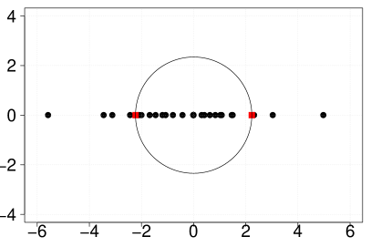
The adaptation proposed here consists in estimating the number of clusters based on the weighted aggregate modularity matrix . Let be the largest (leading) eigenvalue of . The proposed algorithm sets as the number of eigenvalues of higher than . In this paper, we estimate the number of clusters, , to be . This estimation is an upper bound to the number of clusters because the proposed algorithm might leave one or more clusters empty.
Figure 1 displays an example of the proposed strategy by depicting the eigenvalues of the Karate network (Zachary, 1977), whose largest eigenvalue is . The red squares in this figure indicate the points and and a circumference of radius centered at the origin of the Cartesian plane. Most of the black dots, which correspond to the eigenvalues of matrix , are enclosed by the circumference. The proposed algorithm estimates to be the number of eigenvalues higher than , i.e., the number of positive points outside the circumference, which is . Therefore, the upper bound estimation to the number of clusters is .
3.3 Geometric interpretation
Figure 2 illustrates, for a given bipartition of the benchmark Karate network, the geometric interpretation of all the vectors of vertices and clusters. This network has vertices. The positive and negative vectors are shown in Figures 2(a) and 2(b), respectively. In these figures, the vectors of clusters are identified by their labels and the solid and dashed lines distinguish the vertex vectors regarding clusters 1 and 2, respectively.
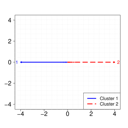
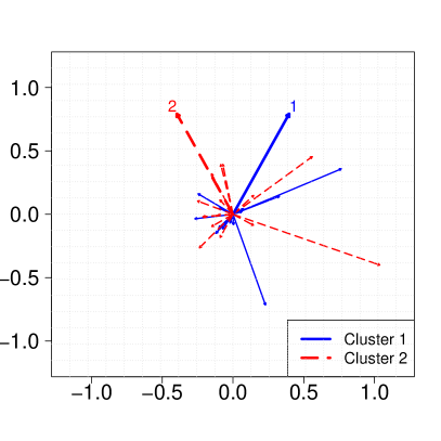
The cluster vectors are the sum of the vertex vectors that compose the clusters. The higher and the lower , and , the higher the modularity. On the one hand, the obvious choice to maximize the magnitude of the positive cluster vectors in Figure 2(a) is to select the vertices whose positive vertex vectors point to the same direction. On the other hand, to minimize the magnitude of the negative cluster vectors in Figure 2(b), the vertices whose negative vertex vectors point to opposite directions should be selected. By comparing Figures 2(a) and 2(b), it is possible to observe that the magnitude of the positive vectors of the clusters is approximately times higher than the magnitude of the negative vectors of the clusters.
3.4 Moving vertices between clusters
Given a partition at hand, some procedures attempt to enhance its quality, which can be evaluated using a fitness function. One way of performing this task is by moving vertices from one cluster to another so that the modified partition has better quality than the previous one. Many studies that employ this type of strategy can be found in the literature, e.g. (Newman, 2006) and (Zhang & Newman, 2015).
Moving a vertex from a cluster to a cluster modifies the fitness function value, i.e., the weighted aggregate modularity. Let the vectors of clusters and , disregarding the contribution of vertex , be defined by , , and .
On the one hand, before moving to cluster , the vectors of clusters are given by and , respectively. On the other hand, before any movement, the vectors of cluster are and . After moving from cluster to , the vectors of the clusters are , , and . Equation (11) presents the change in the weighted aggregate modularity of partition after moving a vertex from a cluster to a cluster .
| (11) |
From Equation (11), it is possible to see that if .
Recently, Zhang & Newman (2015) presented a spectral greedy heuristic to solve the vector partitioning problem considering only positive eigenvalues. In this heuristic, starting from an initial group of vectors, at each iteration, the algorithm moves a vertex to the cluster that results in the largest positive gain in modularity. Concerning both positive and negative eigenvalues, a simple greedy heuristic consists of moving vertex to the cluster that results in the largest value for . Equation (12) defines the choice of .
| (12) |
If , vertex will remain in its original cluster.
4 Proposed Spectral-evolutionary Hybrid Multi-objective Algorithm
This section thoroughly describes the spectral-evolutionary hybrid multi-objective algorithm proposed in this paper and called MOSpecG. MOSpecG is an iterative two-phase algorithm. At the first phase, the weighted aggregate modularity matrix is updated and its eigen-decomposition is performed. At the second phase, a memetic algorithm works based on the information of the vertex vectors – discussed in the earlier section. To a better understanding of the method, Algorithm 1 presents a pseudocode of MOSpecG.
According to Algorithm 1, MOSpecG has as input: an undirected unweighted graph ; the size of the Pareto frontier, ; the number of generations, ; the number of solutions in the population, ; the percentage of solutions from the offspring, ; the number of eigenvalues and eigenvectors to be computed, ; and the number of iterations of the local search procedure, .
In line 1 of Algorithm 1, set is initialized as empty. Consider that the possible values of and are defined in a grid to ensure a good spreading of the solutions in the Pareto frontier approximation. Therefore, the grid spacing is dependent on the number of solutions of the resulting Pareto frontier. In line 2, the grid spacing is assigned to variable in order to define values for . In the sequence, weight is calculated taking as reference, in line 4. From lines 5 to 11, the proposed heuristic creates a new solution to the approximation of the Pareto frontier by optimizing with the current values of and .
In particular, in line 5, the algorithm constructs matrix with weights and according to Equation (5). In line 6, the largest eigenvalues and the associated eigenvectors that compose and are computed using the implicitly restarted Arnoldi method from ARPACK++ library (Lehoucq et al., 1998). In line 7, the leading eigenvalue is assigned to . In lines 8 and 9, MOSpecG estimates the number of clusters, , according to Section 3.2. In line 10, vertex vectors and , , are defined according to Equations (8) and (9), respectively. In line 11, MOSpecG calls the Memetic Algorithm function presented in Algorithm 2 to optimize with weights and . The resulting partition is included in the Pareto frontier approximation in line 12. At the end, Algorithm 1 returns
In the next section, the Memetic Algorithm employed in line 11 of Algorithm 1 is comprehensively discussed.
4.1 Memetic Algorithm
Before going into detail on the algorithm, let us briefly introduce the notations employed in this section.
Let the population of the -ith generation be defined by , where . The individuals from the population of the -ith generation are the partitions , .
Algorithm 2 presents the proposed Memetic Algorithm, whose inputs are: ; ; ; ; the number of clusters, ; and the vertex vectors and , . In line 1 of Algorithm 2, the initial population, i.e., individuals from the first generation, is constructed using the strategy suggested by Zhang & Newman (2015). This strategy selects vertices and assigns each of them to a different cluster ( singletons). Then, the vectors of the selected clusters and , are updated. The remaining vertices are assigned to clusters , where is chosen according to Equation (12).
Figure 3 shows an example of an initial partition of the Karate network. To calculate , we considered . In this figure, each square identifies the cluster label of a vertex of the network.
In line 3, the Memetic Algorithm constructs the offspring of generation , , by applying the genetic operator crossover (Algorithm 3) to the current population . In lines 4 and 5, the genetic operator mutation (Algorithm 4) and a local search procedure (Algorithm 5) update the offspring population. The population of the next generation, , is the population but with the fittest individuals from the offspring replacing the least fit individuals from . In line 8, the algorithm returns the fittest individual from , i.e., individual such that .
4.1.1 Crossover
Algorithm 3 presents the one-way crossover procedure of the Memetic Algorithm, which has as input , , and , . At each iteration , the crossover constructs a new solution for the offspring population, , by combining two solutions from the current population . In line 2, the fitness proportionate roulette method selects two individuals and , , to perform the crossover. In line 3, the algorithm creates an offspring individual as a copy of . In line 4, the method randomly selects a vertex and, in line 5, stores the label of the cluster of in individual .
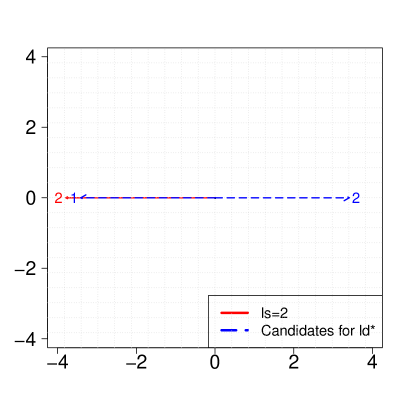
In line 6, the crossover procedure selects the cluster with label from individual as the cluster whose sum of the inner products and is the maximum amongst all , according to Equation (13).
| (13) |
Figure 4 shows an example of the selection performed in line 6 of Algorithm 3. It illustrates the cluster vector with label in individual , as a solid red line, and the cluster vectors with labels in individual – candidates to – as dashed lines. The positive and negative vectors are identified by the label of the clusters and are shown in Figures 4(a) and 4(b), respectively. The conjecture that justifies the selection choice is that the clusters whose vectors point to the same direction have more vertices in common. In this example, the cluster with label from individual is selected because is higher than in individual .
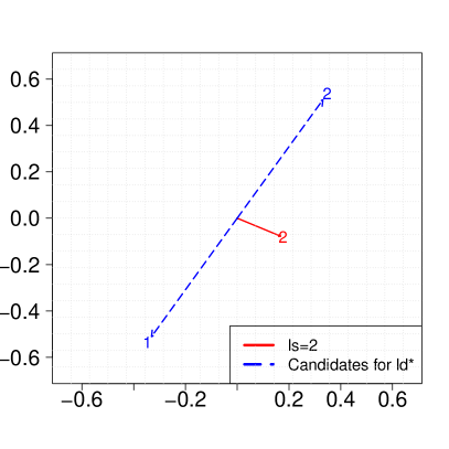
In line 7, the method moves the vertices in the cluster labeled in individual to cluster labeled in individual . For all already belong to the cluster labeled , nothing is done. After each movement, line 8 of Algorithm 3 updates: (i) the weighted aggregate modularity , according to Equation (11), and (ii) the vectors of the clusters involved in the vertex moves in individual , according to Section 3.4. After setting as the offspring individual in line 9, the crossover returns the offspring population .
Figure 5 gives an example of the crossover procedure when . In the example, the offspring individual had a higher weighted aggregate modularity value than the parents and . Let ; the selection of was illustrated in Figure 4. The vertices whose cluster label is on individual are in bold on the partitions. At the offspring individual, which is initially a copy of , these vertices are moved to the group labeled , if they are not yet in this group.
4.1.2 Mutation
Algorithm 4 presents the mutation procedure whose inputs are: the offspring population, ; ; and , . In line 1, a random integer number in the interval is assigned to , which indicates the number of mutations. In line 2, an individual is randomly selected from . In line 3, the algorithm picks vertices from at random to define the set of vertices to be mutated, . Each vertex is assigned to a cluster chosen randomly from individual , in lines 5 and 6. Note that if a cluster is empty, will be assigned to a new cluster. After each movement of a vertex , both and the vectors of cluster are updated in line 8. The mutation procedure halts when all vertices of have been mutated and, then, returns the updated offspring .
Figure 6 presents an example of the mutation procedure on an individual generated to decode a solution for the Karate network. The mutated individual is a result of the modification of the labels of randomly selected vertices.
4.1.3 Local search
Algorithm 5 shows the local search procedure of the introduced Memetic Algorithm, which has as input , , , and , . Each iteration of the local search attempts to improve the modularity value of individuals of offspring by moving vertices to different communities. In line 4, for each individual and each vertex , the local search selects the label such that the relocation of to cluster will result in the largest modularity gain. In line 5, is assigned to cluster , if it does not belong to it yet. After moving , in line 6 of the algorithm, , the vectors of cluster and the vector of the cluster where was found before being moved are updated. Algorithm 5 returns the improved offspring .
Figure 7 illustrates the local search procedure on an individual of the offspring. In this figure, the procedure improved the weighted aggregate modularity of an individual by moving a single vertex to a different cluster.
4.2 Ensemble algorithm
This section introduces an ensemble algorithm that uses information of partitions obtained by MOSpecG to find a single partition that best captures the community structure of a network. Algorithm 6 presents the proposed ensemble algorithm, called SpecG-EC. The algorithm has as input ; ; ; ; ; ; a set of partitions, , and a required threshold, . A partition from is identified by , and represents the solution achieved by MOSpecG for .
Line 1 of Algorithm 6 assigns to every solution from except those by MOSpecG for the pair of values and , i.e., and . Let be a consensus matrix. In lines 2 to 4, is defined according to Lancichinetti & Fortunato (2012): in line 2, receives the number of times that vertices and appear in the same cluster in the partitions from ; in line 3, matrix is normalized; and, in line 4, elements from below a threshold are set to to avoid noisy data. In particular, the step described in line 4 is skipped for , where and .
In order to favor the grouping of vertices that are in the same cluster in the majority of the partitions from , in line 5, the ensemble algorithm adjusts the original graph by adding the consensus matrix to the adjacency matrix.
The ensemble algorithm calculates the eigenvalues and eigenvectors of the original modularity matrix , in line 6. It estimates the number of clusters, , in lines 7 to 9, according to Section 3.2. In line 10, the vertex vectors and , , are created from the eigenvalues and eigenvectors of . Finally, SpecG-EC calls Algorithm 2 to find the partition that maximizes the modularity of the adjusted graph in line 11. The ensemble algorithm returns .
5 Computational Experiments
This section discusses the computational experiments performed with MOSpecG in real and artificial networks. In this section, we refer to MOSpecG for maximizing modularity, i.e., with , as MOSpecG-mod. Both SpecG-EC and MOSpecG were implemented in C++ using the ARPACK++ library222The source code is available at https://github.com/camilapsan/MOSpecG_SpecG.. The following values of the parameters were defined in the algorithms after preliminary tests, reported in A: , , , , and . A single parameter was valued differently in experiments with real networks and artificial networks, which is the number of iterations of the local search, . In the experiments with real networks, the value of was 5, whereas in the experiments with artificial networks, which are much larger than the real networks, was valued 1. All the experiments were run on a computer with an Intel Core i7-4790S processor with 3.20GHz and 8GB of main memory.
The experiments are divided into two parts, each of them with two experiments. The first experiment of the first part shows the results obtained by MOSpecG with real networks. In this experiment, we present the results including the dominated solutions obtained by MOSpecG because some of them had good NMI values. Therefore, we refer to the sets of solutions found by MOSpecG as solution sets rather than Pareto frontier approximations. In the second experiment of the first part, also with real networks, we contrasted the results achieved by SpecG-EC and MOSpecG-mod with those found by the reference graph clustering algorithms: Moga-Net, OSLOM and Infomap. Artificial networks were used in the second part of the computational tests. In the first experiment of the second part, we again present the results achieved by MOSpecG. In the second experiment, we compared the results achieved by SpecG-EC and MOSpecG-mod with those obtained by Moga-Net, OSLOM and Infomap. The codes of the reference algorithms used in the experiments are those provided in the authors’ website.
In all experiments, the expected partitions of the tested networks are known. Thereby, to evaluate the correlation between the solutions found by the algorithms and the ground truth partitions, we used the measure Normalized Mutual Information (NMI) (Shannon, 1948). The NMI values lie in the range and the higher they are, the more correlated is the pair of partitions.
5.1 Experiments with real networks
This section shows the results of the experiments with the real benchmark networks: Karate (Zachary, 1977), Dolphins (Lusseau et al., 2003), Polbooks (Krebs, 2008) and Football (Girvan & Newman, 2002). Table 1 presents the number of vertices and edges in these networks.
| Network | ||||
|---|---|---|---|---|
| Karate | Dolphins | Polbooks | Football | |
| Number of vertices | 34 | 62 | 105 | 115 |
| Number of edges | 78 | 159 | 441 | 613 |
5.1.1 Solution sets found by MOSpecG
Figure 8 exhibits the solution sets achieved by a single execution of MOSpecG for the real benchmark networks. This figure illustrates the trade-offs between the two conflicting objectives. Each point is labeled with the NMI value achieved by the corresponding partitions.
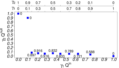
MOSpecG was able to correctly identify the expected partitions of the Karate network for and . On the one hand, MOSpecG achieved the highest NMI values for the Dolphins network when and . On the other hand, it achieved the highest NMI values for the Football and Polbooks networks when and .
Figures 9, 10, 11 and 12 illustrate the partitions found by SpecG-EC and MOSpecG-mod for the Karate, Dolphins, Polbooks and Football networks, respectively. These figures also report the partitions found by MOSpecG with the and values that resulted in the highest NMI values, here referred to as best partitions. Each vertex is identified by its cluster label in these figures.
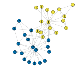
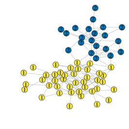
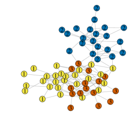
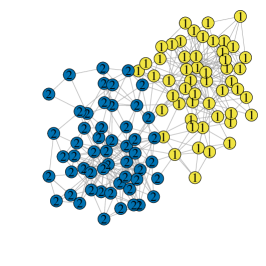


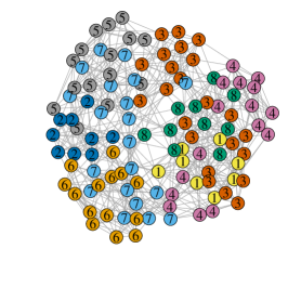
Figure 9 exhibits the expected partition of the Karate network, found by the proposed algorithm. Figure 10 shows that the ensemble and the best partition obtained by MOSpecG for the Dolphins network have the expected number of clusters. The cluster with label from the partition returned by MOSpecG-mod, in Figure 10(b), is merged with the cluster with label in the ensemble partition in Figure 10(a). Figure 11 shows that most of the vertices from clusters with labels and in the partition found by MOSpecG-mod for the Polbooks network are merged in, respectively, clusters with labels and in the ensemble partition obtained by SpecG-EC. None of the partitions found for the Football network in Figure 12 correctly defined the number of clusters.
5.1.2 Comparative analysis
Table 2 reports the average results of ten independent executions of SpecG-EC, MOSpecG-mod, Moga-Net, OSLOM and Infomap to detect communities in real networks. The results presented are the NMI values, the CPU-times in seconds and number of clusters. The standard deviation of the presented values is shown between parentheses. Table 2 also presents the number of clusters in the expected partitions.
| Network | |||||
| Karate | Dolphins | Polbooks | Football | ||
| SpecG-EC | NMI | 1 (0) | 0.889 (0) | 0.565 (0.006) | 0.864 (0.03) |
| CPU-time (s) | 0.172 (0.05) | 0.33 (0.053) | 0.884 (0.131) | 1.377 (0.203) | |
| #Clusters | 2 (0) | 2 (0) | 2.3 (0.483) | 9 (1.054) | |
| MOSpecG-mod | NMI | 1 (0) | 0.662 (0) | 0.485 (0.026) | 0.876 (0.023) |
| CPU-time (s) | 0.015 (0.003) | 0.025 (0.004) | 0.081 (0.015) | 0.129 (0.028) | |
| #Clusters | 2 (0) | 3 (0) | 4.3 (0.483) | 9.4 (0.699) | |
| Moga-Net | NMI | 0.682 (0.047) | 0.538 (0.067) | 0.511 (0.054) | 0.736 (0.048) |
| CPU-time (s) | 7.85 (0.627) | 11.827 (1.255) | 25.231 (2.656) | 28.61 (2.888) | |
| #Clusters | 3.9 (0.316) | 6.1 (1.449) | 5.5 (1.65) | 7.8 (1.033) | |
| OSLOM | NMI | 1 (0) | 0.786 (0.11) | 0.558 (0.017) | 0.916 (0) |
| CPU-time (s) | 0.3 (0.483) | 0.9 (0.568) | 1.2 (0.422) | 0.7 (0.483) | |
| #Clusters | 2 (0) | 2 (0) | 3.7 (0.675) | 11 (0) | |
| Infomap | NMI | 0.699 (0) | 0.519 (0) | 0.537 (0) | 0.924 (0) |
| CPU-time (s) | 0.2 (0.422) | 0.5 (0.527) | 0.4 (0.516) | 0.4 (0.516) | |
| #Clusters | 3 (0) | 6 (0) | 5 (0) | 12 (0) | |
| Expected | #Clusters | 2 | 2 | 3 | 12 |
As can be seen in Table 2, on the one hand, SpecG-EC outperformed Moga-Net in all the networks. On the other hand, MOSpecG-mod only found lower NMI values than Moga-Net for the Polbooks network. Moga-Net and Infomap were the only algorithms which did not obtain the expected partition for the Karate network. SpecG-EC achieved higher NMI values than all the reference algorithms, including MOSpecG-mod, for the Dolphins and Polbooks networks. Furthermore, the number of clusters in the partitions obtained by SpecG-EC and MOSpecG-mod varied at a maximum of and , respectively and on average, when compared to the expected number of clusters. Thereby, there is empirical evidence suggesting the effectiveness of the proposed algorithm in estimating the number of clusters.
The differences between the NMI values reported in Figures 11 and 12 and those presented in Table 2 are due to the fact that the figures only report the results of a single execution, whereas the table shows the average NMI values of ten executions. According to Table 2, the average NMI value of partitions obtained by SpecG-EC for the Polbooks network is only 0.703% lower than the highest NMI value of partitions from the solution set presented in Figure 8(c). Furthermore, SpecG-EC found partitions for Football network whose average NMI value was 5.677% worse than the highest NMI value of partitions from the solution set presented in Figure 8(d).
Table 3 demonstrates details of the experiment performed with the proposed and reference algorithms on network Dolphins333The table additionally reports the results obtained by MOSpecG-MO for each combination of and .. The table presents the NMI and modularity values; the running time in seconds; the number of pairs of vertices which were grouped correctly in the same cluster and incorrectly grouped in the same or different clusters, when compared to the expected partition; and the number and size of the clusters in the partitions obtained by the algorithms. The expected partition of network dolphins has 2 clusters with 42 and 20 vertices.
| Algorithm | NMI | CPU- | Pairs of vertices | Clusters | |||
| time (s) | Correct | Wrong | # | Sizes | |||
| MOSpecG - =0,=1 | 0 | 0 | 0.018 | 1051 | 840 | 1 | 62 |
| MOSpecG - =0.1,=0.9 | 0 | 0 | 0.019 | 1051 | 840 | 1 | 62 |
| MOSpecG - =0.2,=0.8 | 0.486 | 0.378 | 0.025 | 731 | 520 | 2 | 32, 30 |
| MOSpecG - =0.3,=0.7 | 0.514 | 0.391 | 0.025 | 754 | 477 | 2 | 33, 29 |
| MOSpecG - =0.4,=0.6 | 0.662 | 0.483 | 0.024 | 620 | 451 | 3 | 26, 21, 15 |
| MOSpecG - =0.5,=0.5 | 0.662 | 0.483 | 0.022 | 620 | 451 | 3 | 26, 21, 15 |
| MOSpecG - =0.6,=0.4 | 0.581 | 0.518 | 0.026 | 492 | 579 | 4 | 21, 20, 14, 7 |
| MOSpecG - =0.7,=0.3 | 0.889 | 0.379 | 0.025 | 1010 | 61 | 2 | 41, 21 |
| MOSpecG - =0.8,=0.2 | 0.889 | 0.379 | 0.025 | 1010 | 61 | 2 | 41, 21 |
| MOSpecG - =0.9,=0.1 | 0.777 | 0.359 | 0.025 | 991 | 120 | 2 | 42, 20 |
| MOSpecG - =1,=0 | 0 | 0 | 0.024 | 1051 | 840 | 1 | 62 |
| SpecG-EC | 0.889 | 0.379 | 0.281 | 1010 | 61 | 2 | 41, 21 |
| Moga-Net | 0.472 | 0.417 | 13.92 | 532 | 537 | 7 | 31, 10, 6, 6, 4, 3, 2 |
| Infomap | 0.519 | 0.523 | 1 | 417 | 654 | 6 | 21, 17, 12, 7, 3, 2 |
| OSLOM | 0.814 | 0.385 | 1 | 971 | 120 | 2 | 40, 22 |
The results in Table 3 show that the larger and the lower the number of pairs of vertices classified correctly and incorrectly, respectively, the larger the NMI values of the partitions. This table also shows that partitions with higher values of modularity are not necessarily more similar to the expected partitions considering the NMI values, the number and size of the clusters. The partition obtained by SpecG-EC presented the highest NMI value and matched the expected number of clusters, 2. In this partition, exactly one vertex was classified in the wrong cluster. In combining the solutions of MOSpecG by the consensus strategy, SpecG-EC found the partition with the largest NMI. Even though MOSpecG with and and OSLOM identified partitions with 2 clusters and whose numbers of vertices are the expected, 2 vertices were displaced. Both Moga-Net and Infomap identified a large number of clusters, far from the expected.
5.2 Experiments with artificial networks
This experiment used 80 undirected LFR networks (Lancichinetti et al., 2011) with the following characteristics: 1000 vertices; average degree within the range ; small-sized communities, whose number of vertices are in the interval ; large-sized communities, whose number of vertices are in the interval ; and degree of mixture (mixture coefficient) between groups () with values from the set .
5.2.1 Solution sets found by MOSpecG
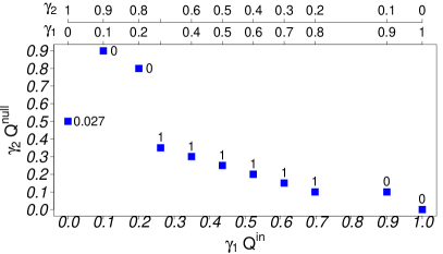
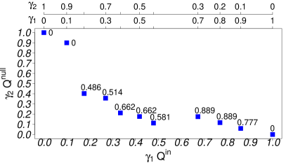
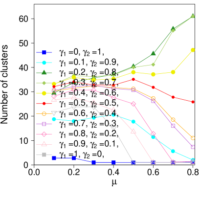
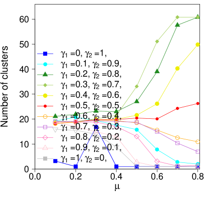
Figures 13 to 17 display the average results of the algorithms applied to the LFR networks (y-axis) by (x-axis). Figures 13(a) and 13(b) present the average NMI values of partitions obtained by MOSpecG for, respectively, the small and large-sized community networks considering each combination of weights and .
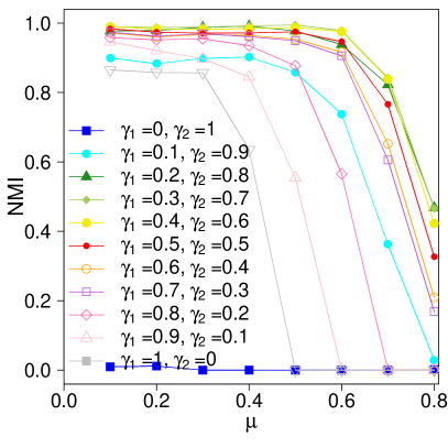
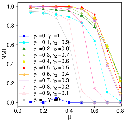
As can be noted in Figures 13(a) and 13(b), the values of and resulted in partitions with the highest average NMI values for the networks with . The proposed heuristic presented competitive results when detecting communities in all networks by optimizing the modularity, i.e., when . The partitions found when considering and failed to identify good quality clusters.
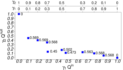
Figures 14(a) and 14(b) show the average number of clusters in the partitions from the solution sets for, respectively, the small and large-sized community networks. Except for the results when , which misidentified the number of clusters, and when , the lower the and the larger the , the larger the number of clusters. Thereby, the number of communities grows with .
5.2.2 Comparative analysis
Figure 15 presents the average NMI values of the partitions found by SpecG-EC, MOSpecG-mod, OSLOM, Infomap and Moga-Net whereas Figure 16 shows the respective average CPU-times for the small and large-sized community networks.
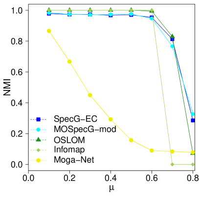
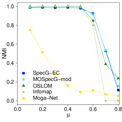
Figure 15 shows that the partitions found by SpecG-EC and MOSpecG-mod had average NMI values higher than those with the largest modularity found by Moga-Net. Moreover, SpecG-EC outperformed MOSpecG-mod, Infomap and OSLOM in the small-sized community networks with, respectively, , and . In the small-sized community networks with , SpecG-EC obtained partitions whose NMI values were higher or equal to . SpecG-EC outperformed MOSpecG-mod, Infomap and OSLOM in large-sized community networks with, respectively, , and , and achieved NMI values of at least in the networks when .
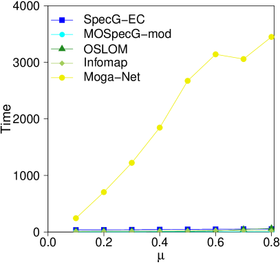
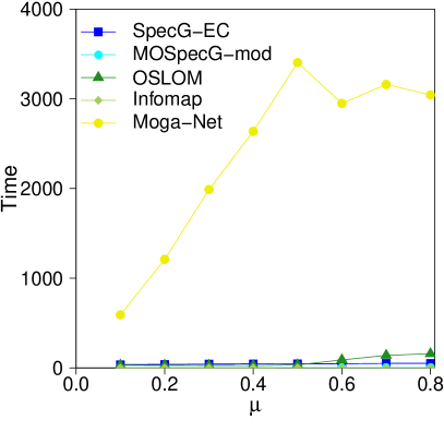
MOSpecG-mod and Infomap were the algorithms with the lowest CPU-times in networks with, respectively, small and large-sized community networks. Nonetheless, SpecG-EC was from to times faster than Moga-Net in all the networks. On the one hand, SpecG-EC was faster than OSLOM in the large-sized community networks with . On the other, it required from to times more than the CPU time required by OSLOM in the remaining networks. Because MOSpecG-mod was approximately times faster than SpecG-EC, it was also faster than OSLOM in all the networks.
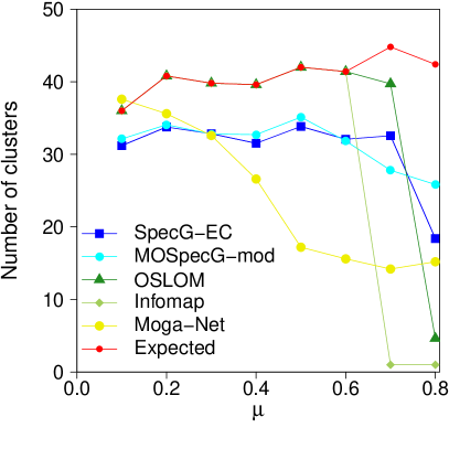
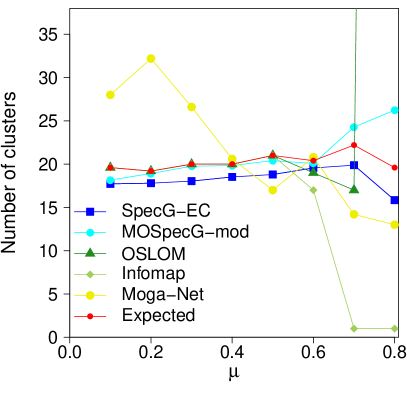
Figure 17 shows the number of clusters obtained by the algorithms in the partitions and in the expected partitions. As can be seen in Figure 17, Moga-Net obtained the partitions with the worst estimation of numbers of clusters with regard to the expected partitions. On the one hand, OSLOM and Infomap found partitions whose number of clusters is exactly the expected in small and large-sized community networks with, respectively, and . On the other hand, as opposed to SpecG-EC and MOSpecG-mod, Infomap failed to identify the number of clusters in the networks with . OSLOM obtained partitions with worse estimations of the number of clusters with regard to the expected partitions than both versions of the proposed algorithm for small and large-sized community networks with, respectively, and . In particular, despite presenting slightly better NMI values than SpecG-EC and MOSpecG-mod for large-sized community network with , OSLOM wrongly identified approximately 381 clusters, on average, more than the expected.
6 Final Remarks and Future Works
This paper presented a novel spectral decomposition of modularity to clustering graphs through a multi-objective memetic algorithm called MOSpecG. In addition, it introduced an ensemble algorithm, here called SpecG-EC, that combines partitions obtained by MOSpecG to provide a single partition.
The results of computational experiments using real and LFR networks showed that SpecG-EC and the version of MOSpecG that maximizes modularity, named MOSpecG-mod, outperformed a multi-objective genetic algorithm found in the literature and presented reasonable running times when compared to reference algorithms. The SpecG-EC and MOSpecG-mod found partitions more similar to the expected ones than state-of-the-art mono-objective algorithms in artificial networks with higher mixture coefficients and satisfactory results in the remaining artificial networks. In particular, SpecG-EC performed better in artificial large-sized community networks and outperformed state-of-the-art mono-objective algorithms in two real networks.
Because SpecG-EC obtained better results than MOSpecG-mod for most of the networks, we can conclude that the ensemble strategy outperformed the maximization of the classical modularity. Nonetheless, SpecG-EC constructs its solution using partitions found by MOSpecG and thus is slower than MOSpecG-mod. The experiments also suggested that both the ensemble and the modularity maximization version of the proposed algorithm provide a reasonable number of clusters in real and artificial networks.
The empirical finding that some partitions obtained by MOSpecG were more similar to the expected partitions than both the modularity maximization and ensemble partitions suggests advantages of studying the duality between the terms of the modularity using multi-objective graph clustering algorithms. In this sense, as future work, we intend to further improve the results achieved by SpecG-EC by studying more effective procedures to select partitions from multi-objective problems for the ensemble.
To combine pairs of vertex partitions, evolutionary algorithms usually match the communities of the different partitions to then perform the crossover operator. The matching of the communities is difficult to establish. In SpecG-EC, however, we propose a spectral analysis to this step. Unfortunately, SpecG-EC does not scale well due to the computational burden in the eigenvalues and eigenvectors computation. Therefore, reducing the computational cost of the spectral decomposition would make this algorithm more effective in detecting communities in larger graphs. As in applications the networks are mostly sparse, a future research direction would be the study of the spectral decomposition of the non-backtracking matrix as the fitness function to reduce the cost of the eigen-decomposition operations of SpecG-EC.
Moreover, it is worth to highlight that in many case-oriented applications, such as the study of metabolic networks, the specialist who performs the cluster analysis prefers to investigate the results of a set of solutions instead of a unique partition. In fact, hierarchical clustering algorithms are widely employed in these studies, primarily due to the unclear definition of clustering and the diversified characteristics of the applications. Therefore, in this sense, MOSpecG can be a powerful tool, since it provides a pool of solutions from the optimization of the bi-objective problem.
Acknowledgments
The authors would like to acknowledge the foundings provided by São Paulo Research Foundation (FAPESP), grant numbers: 2016/22688-2 and 2015/21660-4; and by Conselho Nacional de Desenvolvimento Científico e Tecnológico (CNPq), grant numbers: 306036/2018-5. The authors would also like to thank the anonymous reviewers for their valuable com ments. The second author also thanks Leonardo V. Rosset for giving her a hand.
References
- Amiri et al. (2012) Amiri, B., Hossain, L., & Crawford, J. (2012). A hybrid evolutionary algorithm based on HSA and cls for multi-objective community detection in complex networks. In 2012 IEEE/ACM International Conference on Advances in Social Networks Analysis and Mining (pp. 243–247). https://doi.org/10.1109/ASONAM.2012.49.
- Amiri et al. (2011) Amiri, B., Hossain, L., & Crawford, J. W. (2011). An efficient multiobjective evolutionary algorithm for community detection in social networks. In 2011 IEEE Congress of Evolutionary Computation (CEC) (pp. 2193–2199). https://doi.org/10.1109/CEC.2011.5949886.
- Amiri et al. (2013) Amiri, B., Hossain, L., Crawford, J. W., & Wigand, R. T. (2013). Community detection in complex networks: Multi–objective enhanced firefly algorithm. Knowledge-Based Systems, 46, 1 – 11. https://doi.org/10.1016/j.knosys.2013.01.004.
- Angelini et al. (2007) Angelini, L., Boccaletti, S., Marinazzo, D., Pellicoro, M., & Stramaglia, S. (2007). Identification of network modules by optimization of ratio association. Chaos: An Interdisciplinary Journal of Nonlinear Science, 17, 023114. https://doi.org/10.1063/1.2732162.
- Berry et al. (2011) Berry, J. W., Hendrickson, B., LaViolette, R. A., & Phillips, C. A. (2011). Tolerating the community detection resolution limit with edge weighting. Physical Review E, 83, 056119. https://doi.org/10.1103/PhysRevE.83.056119.
- Brandes et al. (2008) Brandes, U., Delling, D., Gaertler, M., Gorke, R., Hoefer, M., Nikolosk, Z., & Wagner, D. (2008). On modularity clustering. IEEE Transactions on Knowledge and Data Engineering, 20, 172–188. https://doi.org/10.1109/TKDE.2007.190689.
- Carvalho et al. (2014) Carvalho, D. M., Resende, H., & Nascimento, M. C. V. (2014). Modularity maximization adjusted by neural networks. In C. K. Loo, K. S. Yap, K. W. Wong, A. Teoh, & K. Huang (Eds.), Neural Information Processing (pp. 287–294). Cham: Springer volume 8834 of Lecture Notes in Computer Science. https://doi.org/10.1007/978-3-319-12637-1_36.
- Chen et al. (2016) Chen, D., Zou, F., Lu, R., Yu, L., Li, Z., & Wang, J. (2016). Multi-objective optimization of community detection using discrete teaching–learning-based optimization with decomposition. Information Sciences, 369, 402 – 418. https://doi.org/10.1016/j.ins.2016.06.025.
- Cheng et al. (2018) Cheng, F., Cui, T., Su, Y., Niu, Y., & Zhang, X. (2018). A local information based multi-objective evolutionary algorithm for community detection in complex networks. Applied Soft Computing, 69, 357 – 367. https://doi.org/10.1016/j.asoc.2018.04.037.
- Darst et al. (2014) Darst, R. K., Nussinov, Z., & Fortunato, S. (2014). Improving the performance of algorithms to find communities in networks. Physical Review E, 89, 032809. https://doi.org/10.1103/PhysRevE.89.032809.
- De Meo et al. (2013) De Meo, P., Ferrara, E., Fiumara, G., & Provetti, A. (2013). Enhancing community detection using a network weighting strategy. Information Sciences, 222, 648–668. https://doi.org/10.1016/j.ins.2012.08.001.
- Deb et al. (2002) Deb, K., Pratap, A., Agarwal, S., & Meyarivan, T. (2002). A fast and elitist multiobjective genetic algorithm: NSGA-II. IEEE Transactions on Evolutionary Computation, 6, 182–197. https://doi.org/10.1109/4235.996017.
- Ehrgott (2005) Ehrgott, M. (2005). Multicriteria optimization. Berlin, Heidelberg: Springer volume 491 of Lecture Notes in Economics and Mathematical Systems. https://doi.org/10.1007/3-540-27659-9.
- Ferrara et al. (2014) Ferrara, E., Meo, P. D., Catanese, S., & Fiumara, G. (2014). Detecting criminal organizations in mobile phone networks. Expert Systems with Applications, 41, 5733 – 5750. https://doi.org/10.1016/j.eswa.2014.03.024.
- Fortunato & Barthélemy (2007) Fortunato, S., & Barthélemy, M. (2007). Resolution limit in community detection. Proceedings of the National Academy of Sciences, 104, 36. https://doi.org/10.1073/pnas.0605965104.
- Ghaffaripour et al. (2016) Ghaffaripour, Z., Abdollahpouri, A., & Moradi, P. (2016). A multi-objective genetic algorithm for community detection in weighted networks. In 2016 Eighth International Conference on Information and Knowledge Technology (IKT) (pp. 193–199). https://doi.org/10.1109/IKT.2016.7777766.
- Girvan & Newman (2002) Girvan, M., & Newman, M. E. (2002). Community structure in social and biological networks. Proceedings of the National Academy of Sciences, 99, 7821–7826. https://doi.org/10.1073/pnas.122653799.
- Golbeck et al. (2010) Golbeck, J., Grimes, J. M., & Rogers, A. (2010). Twitter use by the us congress. Journal of the Association for Information Science and Technology, 61, 1612–1621. https://doi.org/10.1002/asi.21344.
- Gong et al. (2014) Gong, M., Cai, Q., Chen, X., & Ma, L. (2014). Complex network clustering by multiobjective discrete particle swarm optimization based on decomposition. IEEE Transactions on Evolutionary Computation, 18, 82–97. https://doi.org/10.1109/TEVC.2013.2260862.
- Gong et al. (2013) Gong, M., Chen, X., Ma, L., Zhang, Q., & Jiao, L. (2013). Identification of multi-resolution network structures with multi-objective immune algorithm. Applied Soft Computing, 13, 1705 – 1717. https://doi.org/10.1016/j.asoc.2013.01.018.
- Gong et al. (2011) Gong, M., Hou, T., Fu, B., & Jiao, L. (2011). A non-dominated neighbor immune algorithm for community detection in networks. In Proceedings of the 13th Annual Conference on Genetic and Evolutionary Computation GECCO ’11 (pp. 1627–1634). New York, NY, USA: ACM. https://doi.org/10.1145/2001576.2001796.
- Gong et al. (2012) Gong, M., Ma, L., Zhang, Q., & Jiao, L. (2012). Community detection in networks by using multiobjective evolutionary algorithm with decomposition. Physica A: Statistical Mechanics and its Applications, 391, 4050–4060. https://doi.org/10.1016/j.physa.2012.03.021.
- Kanawati (2015) Kanawati, R. (2015). Empirical evaluation of applying ensemble methods to ego-centred community identification in complex networks. Neurocomputing, 150, 417 – 427. Special Issue on Information Processing and Machine Learning for Applications of Engineering Solving Complex Machine Learning Problems with Ensemble Methods Visual Analytics using Multidimensional Projections. https://doi.org/10.1016/j.neucom.2014.09.042.
- Khadivi et al. (2011) Khadivi, A., Rad, A. A., & Hasler, M. (2011). Network community-detection enhancement by proper weighting. Physical Review E, 83, 046104. https://doi.org/10.1103/PhysRevE.83.046104.
- Krebs (2008) Krebs, V. (2008). A network of books about recent us politics sold by the online bookseller amazon.com. URL: http://www-personal.umich.edu/~mejn/netdata/ Accessed 13 october 2018.
- Krzakala et al. (2013) Krzakala, F., Moore, C., Mossel, E., Neeman, J., Sly, A., Zdeborová, L., & Zhang, P. (2013). Spectral redemption in clustering sparse networks. Proceedings of the National Academy of Sciences, 110, 20935–20940. https://doi.org/10.1073/pnas.1312486110.
- Lancichinetti et al. (2008) Lancichinetti, A., Fortunato, S., & Radicchi, F. (2008). Benchmark graphs for testing community detection algorithms. Physical Review E, 78, 046110. https://doi.org/10.1103/PhysRevE.78.046110.
- Lancichinetti et al. (2011) Lancichinetti, A., Radicchi, F., Ramasco, J. J., & Fortunato, S. (2011). Finding statistically significant communities in networks. PLOS ONE, 6, 1–18. https://doi.org/10.1371/journal.pone.0018961.
- Lancichinetti & Fortunato (2012) Lancichinetti, A., & Fortunato, S. (2012). Consensus clustering in complex networks. Scientific Reports, 2, 336. https://doi.org/10.1038/srep00336.
- Larsson & Moe (2012) Larsson, A. O., & Moe, H. (2012). Studying political microblogging: Twitter users in the 2010 swedish election campaign. New Media & Society, 14, 729–747. https://doi.org/10.1177/1461444811422894.
- Lehoucq et al. (1998) Lehoucq, R. B., Sorensen, D. C., & Yang, C. (1998). ARPACK users’ guide: solution of large-scale eigenvalue problems with implicitly restarted arnoldi methods. SIAM volume 6 of Software, Environments, Tools. https://doi.org/10.1137/1.9780898719628.
- Li et al. (2012) Li, Y., Chen, J., Liu, R., & Wu, J. (2012). A spectral clustering-based adaptive hybrid multi-objective harmony search algorithm for community detection. In 2012 IEEE Congress on Evolutionary Computation (pp. 1–8). IEEE. https://doi.org/10.1109/CEC.2012.6253013.
- Liang et al. (2014) Liang, Z.-W., Li, J.-P., Yang, F., & Petropulu, A. (2014). Detecting community structure using label propagation with consensus weight in complex network. Chinese Physics B, 23, 098902. https://doi.org/10.1088/1674-1056/23/9/098902.
- Lusseau et al. (2003) Lusseau, D., Schneider, K., Boisseau, O., Haase, P., Slooten, E., & Dawson, S. (2003). The bottlenose dolphin community of doubtful sound features a large proportion of long-lasting associations. Behavioral Ecology and Sociobiology, 54, 396–405. https://doi.org/10.1007/s00265-003-0651-y.
- Nascimento et al. (2009) Nascimento, M. C. V., de Toledo, F. M. B., & Carvalho, A. C. P. L. F. (2009). Consensus clustering using spectral theory. In M. Köppen, N. Kasabov, & G. Coghill (Eds.), Advances in Neuro-Information Processing (pp. 461–468). Berlin, Heidelberg: Springer volume 5506 of Lecture Notes in Computer Science. https://doi.org/10.1007/978-3-642-02490-0_57.
- Newman & Girvan (2004) Newman, M. E. J., & Girvan, M. (2004). Finding and evaluating community structure in networks. Physical Review E, 69, 026113. https://doi.org/10.1103/PhysRevE.69.026113.
- Newman (2006) Newman, M. E. J. (2006). Finding community structure in networks using the eigenvectors of matrices. Physical Review E, 74, 036104. https://doi.org/10.1103/PhysRevE.74.036104.
- Pizzuti (2008) Pizzuti, C. (2008). GA-NET: A genetic algorithm for community detection in social networks. In International Conference on Parallel Problem Solving from Nature (pp. 1081–1090). Springer. https://doi.org/10.1007/978-3-540-87700-4_107.
- Pizzuti (2009) Pizzuti, C. (2009). A multi-objective genetic algorithm for community detection in networks. In 2009 21st IEEE International Conference on Tools with Artificial Intelligence (pp. 379–386). IEEE. https://doi.org/10.1109/ICTAI.2009.58.
- Pizzuti (2012) Pizzuti, C. (2012). A multiobjective genetic algorithm to find communities in complex networks. IEEE Transactions on Evolutionary Computation, 16, 418–430. https://doi.org/10.1109/TEVC.2011.2161090.
- Pourkazemi & Keyvanpour (2017) Pourkazemi, M., & Keyvanpour, M. R. (2017). Community detection in social network by using a multi-objective evolutionary algorithm. Intelligent Data Analysis, 21, 385–409. https://doi.org/10.3233/IDA-150429.
- Raghavan et al. (2007) Raghavan, U. N., Albert, R., & Kumara, S. (2007). Near linear time algorithm to detect community structures in large-scale networks. Physical Review E, 76, 036106. https://doi.org/10.1103/PhysRevE.76.036106.
- Rahimi et al. (2018) Rahimi, S., Abdollahpouri, A., & Moradi, P. (2018). A multi-objective particle swarm optimization algorithm for community detection in complex networks. Swarm and Evolutionary Computation, 39, 297 – 309. https://doi.org/10.1016/j.swevo.2017.10.009.
- Reichardt & Bornholdt (2006) Reichardt, J., & Bornholdt, S. (2006). Statistical mechanics of community detection. Physical Review E, 74, 016110. https://doi.org/10.1103/PhysRevE.74.016110.
- Rosvall & Bergstrom (2008) Rosvall, M., & Bergstrom, C. T. (2008). Maps of random walks on complex networks reveal community structure. Proceedings of the National Academy of Sciences, 105, 1118–1123. https://doi.org/10.1073/pnas.0706851105.
- Santos et al. (2016) Santos, C. P., Carvalho, D. M., & Nascimento, M. C. (2016). A consensus graph clustering algorithm for directed networks. Expert Systems with Applications, 54, 121–135. https://doi.org/10.1016/j.eswa.2016.01.026.
- Shang et al. (2016) Shang, R., Luo, S., Zhang, W., Stolkin, R., & Jiao, L. (2016). A multiobjective evolutionary algorithm to find community structures based on affinity propagation. Physica A: Statistical Mechanics and its Applications, 453, 203 – 227. https://doi.org/10.1016/j.physa.2016.02.020.
- Shannon (1948) Shannon, C. E. (1948). A mathematical theory of communication. Bell System Technical Journal, 27, 379–423. https://doi.org/10.1002/j.1538-7305.1948.tb01338.x.
- Shi et al. (2012) Shi, C., Yan, Z., Cai, Y., & Wu, B. (2012). Multi-objective community detection in complex networks. Applied Soft Computing, 12, 850–859. https://doi.org/10.1016/j.asoc.2011.10.005.
- Wei & Cheng (1991) Wei, Y.-C., & Cheng, C.-K. (1991). Ratio cut partitioning for hierarchical designs. IEEE Transactions on Computer-Aided Design of Integrated Circuits and Systems, 10, 911–921. https://doi.org/10.1109/43.87601.
- Xu et al. (2015) Xu, B., Qi, J., Zhou, C., Hu, X., Xu, B., & Sun, Y. (2015). Hybrid self-adaptive algorithm for community detection in complex networks. Mathematical Problems in Engineering, 2015. https://doi.org/10.1155/2015/273054.
- Zachary (1977) Zachary, W. W. (1977). An information flow model for conflict and fission in small groups. Journal of Anthropological Research, 33, 452–473. https://doi.org/10.1086/jar.33.4.3629752.
- Žalik & Žalik (2018) Žalik, K. R., & Žalik, B. (2018). Multi-objective evolutionary algorithm using problem-specific genetic operators for community detection in networks. Neural Computing and Applications, 30, 2907–2920. https://doi.org/10.1007/s00521-017-2884-0.
- Zhang & Newman (2015) Zhang, X., & Newman, M. (2015). Multiway spectral community detection in networks. Physical Review E, 92, 052808. https://doi.org/10.1103/PhysRevE.92.052808.
- Zhou et al. (2016) Zhou, X., Liu, Y., & Li, B. (2016). A multi-objective discrete cuckoo search algorithm with local search for community detection in complex networks. Modern Physics Letters B, 30, 1650080. https://doi.org/10.1142/S0217984916500809.
- Zhu et al. (2008) Zhu, Z., Wang, C., Ma, L., Pan, Y., & Ding, Z. (2008). Scalable community discovery of large networks. WAIM ’08 Proceedings of the 2008 The Ninth International Conference on Web-Age Information Management, (pp. 381–388). https://doi.org/10.1109/WAIM.2008.13.
- Zou et al. (2019) Zou, F., Chen, D., Huang, D.-S., Lu, R., & Wang, X. (2019). Inverse modelling-based multi-objective evolutionary algorithm with decomposition for community detection in complex networks. Physica A: Statistical Mechanics and its Applications, 513, 662 – 674. https://doi.org/10.1016/j.physa.2018.08.077.
- Zou et al. (2017) Zou, F., Chen, D., Li, S., Lu, R., & Lin, M. (2017). Community detection in complex networks: Multi-objective discrete backtracking search optimization algorithm with decomposition. Applied Soft Computing, 53, 285 – 295. https://doi.org/10.1016/j.asoc.2017.01.005.
Appendix A Setting up parameters
In this appendix, we present the preliminary experiments carried out using LFR and real networks to fine-tune the parameters of the proposed algorithms. First, we identified the best parameters for MOSpecG-mod, which is MOSpecG when maximizing the classical version of the modularity measure. After these parameters have been defined, we decide the best value of the parameters and of SpecG-EC.
Tables 4, 5, 6 and 7 present the results achieved by MOSpecG-mod to detect communities in LFR networks. Tables 8 and 9 demonstrate the average results of 10 independent executions of MOSpecG-mod to find partitions of the real networks Karate (Zachary, 1977), Dolphins (Lusseau et al., 2003), Polbooks (Krebs, 2008) and Football (Girvan & Newman, 2002). These tables show the NMI values of the partitions with respect to the expected ones and the respective execution times in seconds of MOSpecG-mod. All possible combinations of the following parameter values were considered in these experiments: , , , and . In addition, Tables 4, 5, 6 and 7 report the average (AVG), maximum (MAX) and minimum (MIN) NMI values and execution times in detecting communities in the networks with each mixture coefficient value. The shades of gray used as background colors of the table cells are in accordance with the NMI values.
In Tables 10 and 11, we show the Pearson correlation coefficients444The Pearson correlation coefficient assesses the linear correlation between two variables. It is valued from -1 to 1, where -1 and 1 indicate a perfect negative and positive linear correlation, respectively; the value 0 indicates no linear correlation between the pair of variables. between the MOSpecG-mod parameters and (i) the NMI values of the partitions with respect to the expected partitioning of LFR networks considering each possible value of , and (ii) the corresponding average (AVG), maximum (MAX) and minimum (MIN) execution times. Table 12 presents the Pearson correlation coefficients between the MOSpecG-mod parameters and the NMI values and execution time in seconds for real networks.
As expected, the parameter , which refers to the number of eigenvalues and eigenvectors used in the spectral relaxation, presented the highest positive correlation coefficient values with respect to the execution times. On the one hand, the correlation coefficients between and the NMI values were lower than for small- and large-sized community networks with, respectively, and . On the other, when considering networks with , the correlation coefficients between and the NMI values ranged from to . The Pearson correlations between and the NMI values of the real network partitions were also conflicting: their values were , and for Karate, Polbooks and Football networks, respectively. Therefore, in spite of being difficult to draw general conclusions by these results, we remark that the NMI values of partitions of LFR networks increased with only in networks with high mixture coefficients.
In addition, according to Tables 10 and 11, one can also observe that the correlations between and the NMI values of the partitions of LFR networks with were at least . Nevertheless, the correlations were and when considering small- and large-sized community networks with . One conjecture that might justify the negative correlations in such cases is that MOSpecG-mod has more chance of selecting high-quality partitions more often for the crossover operator when is lower. Tables 10, 11 and 12 also show that regardless the network under consideration the execution time increases alongside .
In the parameter-tuning, we selected the set of parameters for MOSpecG-mod to obtain partitions with satisfactory NMI values taking a reasonable running time. In line with this, parameters and received values and , respectively. Nonetheless, we recommend setting higher values for and when the networks under study have high and low mixture coefficients, respectively.
The correlation coefficients between parameter and the NMI values did not present a clear pattern when considering the LFR networks showed in Tables 10 and 11. On the one hand, these correlations were at least when . On the other, they were and respectively for small- and large-community size networks with . Since increasing does not augment the execution times, we adopted the median value to this parameter, .
and did not have a strong correlation with the NMI values for the LFR networks even though the execution times increased alongside and . When considering the real networks, however, the correlations between and the NMI values shown in Table 12 ranged from to . We therefore considered to enhance the robustness of MOSpecG-mod. Because the parameter only showed a strong correlation with the NMI value of the partition obtained to the Polbooks network, we used the lowest value of , 1, to carry out the experiments with the LFR networks. Nevertheless, in small networks such as the real networks tested in the experiments presented in this paper, we recommend increasing since the computational time is significantly low in practice.
Therefore, we chose the following values of parameters: , , . The parameter was 1 in tests with LFR networks and 5 in the experiments with real networks.
Tables 13, 14 and 15 show the NMI values of the partitions obtained by SpecG-EC in small- and large-sized community networks with different mixture coefficients and in real networks. This experiment was performed by fixing the values of and at values decided on the previous parameter tuning experiments and considering the respective combination of the remaining parameters: and . In addition, Tables 13 and 14 report the average (AVG), maximum (MAX) and minimum (MIN) values of NMI and execution times in seconds of the consensus step in SpecG-EC considering the networks with different mixture coefficients. Even though we did not report the running times of SpecG-EC to obtain the partitions required to define the consensus partition, the average execution times increase alongside and .
According to Tables 13 and 14, the highest NMI values were achieved when and . Considering Table 15, the highest NMI values were obtained when and . The NMI values of partitions of the LFR networks with when were on average only worse than the NMI values of partitions when . As considering the real networks SpecG-EC performed better when was fixed at 0.5, we assigned 0.5 to parameter .
| Parameters | NMI | Time (s) | ||||||||||||||||
|---|---|---|---|---|---|---|---|---|---|---|---|---|---|---|---|---|---|---|
| 0.1 | 0.2 | 0.3 | 0.4 | 0.5 | 0.6 | 0.7 | 0.8 | AVG | MAX | MIN | AVG | MAX | MIN | |||||
| 10 | 5 | 10 | 10 | \collectcell 0 .901\endcollectcell | \collectcell 0 .882\endcollectcell | \collectcell 0 .887\endcollectcell | \collectcell 0 .907\endcollectcell | \collectcell 0 .853\endcollectcell | \collectcell 0 .774\endcollectcell | \collectcell 0 .55\endcollectcell | \collectcell 0 .323\endcollectcell | \collectcell 0 .76\endcollectcell | \collectcell 0 .907\endcollectcell | \collectcell 0 .323\endcollectcell | 3.939 | 4.563 | 3.396 | |
| 10 | 5 | 10 | 50 | \collectcell 0 .886\endcollectcell | \collectcell 0 .882\endcollectcell | \collectcell 0 .897\endcollectcell | \collectcell 0 .896\endcollectcell | \collectcell 0 .844\endcollectcell | \collectcell 0 .769\endcollectcell | \collectcell 0 .55\endcollectcell | \collectcell 0 .327\endcollectcell | \collectcell 0 .756\endcollectcell | \collectcell 0 .897\endcollectcell | \collectcell 0 .327\endcollectcell | 5.86 | 6.632 | 5.321 | |
| 10 | 5 | 10 | 10 | \collectcell 0 .849\endcollectcell | \collectcell 0 .838\endcollectcell | \collectcell 0 .851\endcollectcell | \collectcell 0 .831\endcollectcell | \collectcell 0 .781\endcollectcell | \collectcell 0 .697\endcollectcell | \collectcell 0 .589\endcollectcell | \collectcell 0 .469\endcollectcell | \collectcell 0 .738\endcollectcell | \collectcell 0 .851\endcollectcell | \collectcell 0 .469\endcollectcell | 11.346 | 13.567 | 7.686 | |
| 10 | 5 | 10 | 50 | \collectcell 0 .841\endcollectcell | \collectcell 0 .838\endcollectcell | \collectcell 0 .858\endcollectcell | \collectcell 0 .83\endcollectcell | \collectcell 0 .781\endcollectcell | \collectcell 0 .69\endcollectcell | \collectcell 0 .597\endcollectcell | \collectcell 0 .465\endcollectcell | \collectcell 0 .738\endcollectcell | \collectcell 0 .858\endcollectcell | \collectcell 0 .465\endcollectcell | 28.864 | 36.643 | 13.642 | |
| 10 | 5 | 10 | 10 | \collectcell 0 .821\endcollectcell | \collectcell 0 .81\endcollectcell | \collectcell 0 .822\endcollectcell | \collectcell 0 .798\endcollectcell | \collectcell 0 .761\endcollectcell | \collectcell 0 .685\endcollectcell | \collectcell 0 .634\endcollectcell | \collectcell 0 .548\endcollectcell | \collectcell 0 .735\endcollectcell | \collectcell 0 .822\endcollectcell | \collectcell 0 .548\endcollectcell | 20.778 | 28.898 | 12.412 | |
| 10 | 5 | 10 | 50 | \collectcell 0 .829\endcollectcell | \collectcell 0 .811\endcollectcell | \collectcell 0 .82\endcollectcell | \collectcell 0 .803\endcollectcell | \collectcell 0 .758\endcollectcell | \collectcell 0 .695\endcollectcell | \collectcell 0 .629\endcollectcell | \collectcell 0 .542\endcollectcell | \collectcell 0 .736\endcollectcell | \collectcell 0 .829\endcollectcell | \collectcell 0 .542\endcollectcell | 60.065 | 91.883 | 22.256 | |
| 10 | 5 | 40 | 10 | \collectcell 0 .985\endcollectcell | \collectcell 0 .98\endcollectcell | \collectcell 0 .98\endcollectcell | \collectcell 0 .969\endcollectcell | \collectcell 0 .968\endcollectcell | \collectcell 0 .943\endcollectcell | \collectcell 0 .767\endcollectcell | \collectcell 0 .331\endcollectcell | \collectcell 0 .865\endcollectcell | \collectcell 0 .985\endcollectcell | \collectcell 0 .331\endcollectcell | 1.865 | 2.118 | 1.689 | |
| 10 | 5 | 40 | 50 | \collectcell 0 .979\endcollectcell | \collectcell 0 .977\endcollectcell | \collectcell 0 .979\endcollectcell | \collectcell 0 .972\endcollectcell | \collectcell 0 .969\endcollectcell | \collectcell 0 .952\endcollectcell | \collectcell 0 .79\endcollectcell | \collectcell 0 .339\endcollectcell | \collectcell 0 .87\endcollectcell | \collectcell 0 .979\endcollectcell | \collectcell 0 .339\endcollectcell | 4.136 | 4.53 | 3.498 | |
| 10 | 5 | 40 | 10 | \collectcell 0 .981\endcollectcell | \collectcell 0 .98\endcollectcell | \collectcell 0 .999\endcollectcell | \collectcell 0 .999\endcollectcell | \collectcell 0 .996\endcollectcell | \collectcell 0 .99\endcollectcell | \collectcell 0 .919\endcollectcell | \collectcell 0 .409\endcollectcell | \collectcell 0 .909\endcollectcell | \collectcell 0 .999\endcollectcell | \collectcell 0 .409\endcollectcell | 10.05 | 13.067 | 5.876 | |
| 10 | 5 | 40 | 50 | \collectcell 0 .98\endcollectcell | \collectcell 0 .983\endcollectcell | \collectcell 0 .997\endcollectcell | \collectcell 0 .999\endcollectcell | \collectcell 0 .999\endcollectcell | \collectcell 0 .998\endcollectcell | \collectcell 0 .937\endcollectcell | \collectcell 0 .411\endcollectcell | \collectcell 0 .913\endcollectcell | \collectcell 0 .999\endcollectcell | \collectcell 0 .411\endcollectcell | 29.572 | 38.344 | 11.395 | |
| 10 | 5 | 40 | 10 | \collectcell 0 .988\endcollectcell | \collectcell 0 .987\endcollectcell | \collectcell 0 .998\endcollectcell | \collectcell 0 .999\endcollectcell | \collectcell 1\endcollectcell | \collectcell 0 .997\endcollectcell | \collectcell 0 .903\endcollectcell | \collectcell 0 .469\endcollectcell | \collectcell 0 .918\endcollectcell | \collectcell 1\endcollectcell | \collectcell 0 .469\endcollectcell | 20.374 | 27.569 | 12.813 | |
| 10 | 5 | 40 | 50 | \collectcell 0 .986\endcollectcell | \collectcell 0 .987\endcollectcell | \collectcell 1\endcollectcell | \collectcell 1\endcollectcell | \collectcell 1\endcollectcell | \collectcell 0 .999\endcollectcell | \collectcell 0 .959\endcollectcell | \collectcell 0 .456\endcollectcell | \collectcell 0 .923\endcollectcell | \collectcell 1\endcollectcell | \collectcell 0 .456\endcollectcell | 61.71 | 100.439 | 22.056 | |
| 10 | 5 | 70 | 10 | \collectcell 0 .981\endcollectcell | \collectcell 0 .981\endcollectcell | \collectcell 0 .973\endcollectcell | \collectcell 0 .969\endcollectcell | \collectcell 0 .969\endcollectcell | \collectcell 0 .953\endcollectcell | \collectcell 0 .749\endcollectcell | \collectcell 0 .33\endcollectcell | \collectcell 0 .863\endcollectcell | \collectcell 0 .981\endcollectcell | \collectcell 0 .33\endcollectcell | 2.335 | 2.622 | 1.896 | |
| 10 | 5 | 70 | 50 | \collectcell 0 .984\endcollectcell | \collectcell 0 .981\endcollectcell | \collectcell 0 .98\endcollectcell | \collectcell 0 .969\endcollectcell | \collectcell 0 .973\endcollectcell | \collectcell 0 .953\endcollectcell | \collectcell 0 .779\endcollectcell | \collectcell 0 .334\endcollectcell | \collectcell 0 .869\endcollectcell | \collectcell 0 .984\endcollectcell | \collectcell 0 .334\endcollectcell | 4.728 | 5.086 | 3.979 | |
| 10 | 5 | 70 | 10 | \collectcell 0 .983\endcollectcell | \collectcell 0 .98\endcollectcell | \collectcell 0 .997\endcollectcell | \collectcell 1\endcollectcell | \collectcell 0 .997\endcollectcell | \collectcell 0 .99\endcollectcell | \collectcell 0 .916\endcollectcell | \collectcell 0 .414\endcollectcell | \collectcell 0 .91\endcollectcell | \collectcell 1\endcollectcell | \collectcell 0 .414\endcollectcell | 10.37 | 12.769 | 6.580 | |
| 10 | 5 | 70 | 50 | \collectcell 0 .981\endcollectcell | \collectcell 0 .983\endcollectcell | \collectcell 0 .999\endcollectcell | \collectcell 1\endcollectcell | \collectcell 0 .996\endcollectcell | \collectcell 0 .996\endcollectcell | \collectcell 0 .942\endcollectcell | \collectcell 0 .419\endcollectcell | \collectcell 0 .915\endcollectcell | \collectcell 1\endcollectcell | \collectcell 0 .419\endcollectcell | 27.99 | 40.331 | 11.746 | |
| 10 | 5 | 70 | 10 | \collectcell 0 .988\endcollectcell | \collectcell 0 .99\endcollectcell | \collectcell 0 .998\endcollectcell | \collectcell 0 .999\endcollectcell | \collectcell 0 .999\endcollectcell | \collectcell 0 .997\endcollectcell | \collectcell 0 .901\endcollectcell | \collectcell 0 .464\endcollectcell | \collectcell 0 .917\endcollectcell | \collectcell 0 .999\endcollectcell | \collectcell 0 .464\endcollectcell | 19.707 | 26.755 | 13.802 | |
| 10 | 5 | 70 | 50 | \collectcell 0 .983\endcollectcell | \collectcell 0 .988\endcollectcell | \collectcell 0 .999\endcollectcell | \collectcell 0 .999\endcollectcell | \collectcell 1\endcollectcell | \collectcell 0 .999\endcollectcell | \collectcell 0 .962\endcollectcell | \collectcell 0 .447\endcollectcell | \collectcell 0 .922\endcollectcell | \collectcell 1\endcollectcell | \collectcell 0 .447\endcollectcell | 57.508 | 92.233 | 20.299 | |
| 10 | 10 | 10 | 10 | \collectcell 0 .987\endcollectcell | \collectcell 0 .986\endcollectcell | \collectcell 0 .98\endcollectcell | \collectcell 0 .973\endcollectcell | \collectcell 0 .97\endcollectcell | \collectcell 0 .948\endcollectcell | \collectcell 0 .749\endcollectcell | \collectcell 0 .329\endcollectcell | \collectcell 0 .865\endcollectcell | \collectcell 0 .987\endcollectcell | \collectcell 0 .329\endcollectcell | 2.466 | 2.823 | 2.217 | |
| 10 | 10 | 10 | 50 | \collectcell 0 .988\endcollectcell | \collectcell 0 .984\endcollectcell | \collectcell 0 .982\endcollectcell | \collectcell 0 .976\endcollectcell | \collectcell 0 .977\endcollectcell | \collectcell 0 .958\endcollectcell | \collectcell 0 .792\endcollectcell | \collectcell 0 .339\endcollectcell | \collectcell 0 .875\endcollectcell | \collectcell 0 .988\endcollectcell | \collectcell 0 .339\endcollectcell | 6.916 | 7.535 | 5.380 | |
| 10 | 10 | 10 | 10 | \collectcell 0 .987\endcollectcell | \collectcell 0 .985\endcollectcell | \collectcell 0 .998\endcollectcell | \collectcell 0 .999\endcollectcell | \collectcell 0 .996\endcollectcell | \collectcell 0 .992\endcollectcell | \collectcell 0 .908\endcollectcell | \collectcell 0 .418\endcollectcell | \collectcell 0 .91\endcollectcell | \collectcell 0 .999\endcollectcell | \collectcell 0 .418\endcollectcell | 13.816 | 17.218 | 7.192 | |
| 10 | 10 | 10 | 50 | \collectcell 0 .985\endcollectcell | \collectcell 0 .984\endcollectcell | \collectcell 0 .998\endcollectcell | \collectcell 1\endcollectcell | \collectcell 1\endcollectcell | \collectcell 0 .996\endcollectcell | \collectcell 0 .95\endcollectcell | \collectcell 0 .419\endcollectcell | \collectcell 0 .917\endcollectcell | \collectcell 1\endcollectcell | \collectcell 0 .419\endcollectcell | 49.406 | 66.762 | 18.639 | |
| 10 | 10 | 10 | 10 | \collectcell 0 .985\endcollectcell | \collectcell 0 .99\endcollectcell | \collectcell 0 .999\endcollectcell | \collectcell 0 .998\endcollectcell | \collectcell 0 .999\endcollectcell | \collectcell 0 .997\endcollectcell | \collectcell 0 .887\endcollectcell | \collectcell 0 .47\endcollectcell | \collectcell 0 .916\endcollectcell | \collectcell 0 .999\endcollectcell | \collectcell 0 .47\endcollectcell | 28.757 | 42.609 | 13.662 | |
| 10 | 10 | 10 | 50 | \collectcell 0 .987\endcollectcell | \collectcell 0 .99\endcollectcell | \collectcell 1\endcollectcell | \collectcell 1\endcollectcell | \collectcell 1\endcollectcell | \collectcell 1\endcollectcell | \collectcell 0 .947\endcollectcell | \collectcell 0 .461\endcollectcell | \collectcell 0 .923\endcollectcell | \collectcell 1\endcollectcell | \collectcell 0 .461\endcollectcell | 108.069 | 175.175 | 36.357 | |
| 10 | 10 | 40 | 10 | \collectcell 0 .986\endcollectcell | \collectcell 0 .98\endcollectcell | \collectcell 0 .982\endcollectcell | \collectcell 0 .976\endcollectcell | \collectcell 0 .973\endcollectcell | \collectcell 0 .95\endcollectcell | \collectcell 0 .78\endcollectcell | \collectcell 0 .331\endcollectcell | \collectcell 0 .87\endcollectcell | \collectcell 0 .986\endcollectcell | \collectcell 0 .331\endcollectcell | 2.391 | 2.648 | 2.184 | |
| 10 | 10 | 40 | 50 | \collectcell 0 .989\endcollectcell | \collectcell 0 .983\endcollectcell | \collectcell 0 .983\endcollectcell | \collectcell 0 .982\endcollectcell | \collectcell 0 .973\endcollectcell | \collectcell 0 .95\endcollectcell | \collectcell 0 .793\endcollectcell | \collectcell 0 .337\endcollectcell | \collectcell 0 .874\endcollectcell | \collectcell 0 .989\endcollectcell | \collectcell 0 .337\endcollectcell | 7.228 | 8.476 | 5.596 | |
| 10 | 10 | 40 | 10 | \collectcell 0 .986\endcollectcell | \collectcell 0 .985\endcollectcell | \collectcell 0 .999\endcollectcell | \collectcell 0 .999\endcollectcell | \collectcell 1\endcollectcell | \collectcell 0 .992\endcollectcell | \collectcell 0 .919\endcollectcell | \collectcell 0 .411\endcollectcell | \collectcell 0 .911\endcollectcell | \collectcell 1\endcollectcell | \collectcell 0 .411\endcollectcell | 14.935 | 18.538 | 8.249 | |
| 10 | 10 | 40 | 50 | \collectcell 0 .984\endcollectcell | \collectcell 0 .983\endcollectcell | \collectcell 1\endcollectcell | \collectcell 0 .999\endcollectcell | \collectcell 0 .999\endcollectcell | \collectcell 0 .999\endcollectcell | \collectcell 0 .942\endcollectcell | \collectcell 0 .411\endcollectcell | \collectcell 0 .915\endcollectcell | \collectcell 1\endcollectcell | \collectcell 0 .411\endcollectcell | 49.835 | 64.276 | 19.583 | |
| 10 | 10 | 40 | 10 | \collectcell 0 .987\endcollectcell | \collectcell 0 .99\endcollectcell | \collectcell 1\endcollectcell | \collectcell 0 .999\endcollectcell | \collectcell 0 .999\endcollectcell | \collectcell 0 .999\endcollectcell | \collectcell 0 .929\endcollectcell | \collectcell 0 .482\endcollectcell | \collectcell 0 .923\endcollectcell | \collectcell 1\endcollectcell | \collectcell 0 .482\endcollectcell | 28.679 | 44.118 | 12.843 | |
| 10 | 10 | 40 | 50 | \collectcell 0 .989\endcollectcell | \collectcell 0 .99\endcollectcell | \collectcell 1\endcollectcell | \collectcell 1\endcollectcell | \collectcell 1\endcollectcell | \collectcell 0 .999\endcollectcell | \collectcell 0 .969\endcollectcell | \collectcell 0 .46\endcollectcell | \collectcell 0 .926\endcollectcell | \collectcell 1\endcollectcell | \collectcell 0 .46\endcollectcell | 106.041 | 175.882 | 33.539 | |
| 10 | 10 | 70 | 10 | \collectcell 0 .992\endcollectcell | \collectcell 0 .979\endcollectcell | \collectcell 0 .979\endcollectcell | \collectcell 0 .976\endcollectcell | \collectcell 0 .975\endcollectcell | \collectcell 0 .955\endcollectcell | \collectcell 0 .754\endcollectcell | \collectcell 0 .326\endcollectcell | \collectcell 0 .867\endcollectcell | \collectcell 0 .992\endcollectcell | \collectcell 0 .326\endcollectcell | 2.527 | 3.088 | 2.236 | |
| 10 | 10 | 70 | 50 | \collectcell 0 .984\endcollectcell | \collectcell 0 .982\endcollectcell | \collectcell 0 .982\endcollectcell | \collectcell 0 .973\endcollectcell | \collectcell 0 .972\endcollectcell | \collectcell 0 .956\endcollectcell | \collectcell 0 .788\endcollectcell | \collectcell 0 .338\endcollectcell | \collectcell 0 .872\endcollectcell | \collectcell 0 .984\endcollectcell | \collectcell 0 .338\endcollectcell | 6.912 | 7.577 | 5.488 | |
| 10 | 10 | 70 | 10 | \collectcell 0 .986\endcollectcell | \collectcell 0 .981\endcollectcell | \collectcell 0 .999\endcollectcell | \collectcell 0 .999\endcollectcell | \collectcell 0 .998\endcollectcell | \collectcell 0 .995\endcollectcell | \collectcell 0 .919\endcollectcell | \collectcell 0 .411\endcollectcell | \collectcell 0 .911\endcollectcell | \collectcell 0 .999\endcollectcell | \collectcell 0 .411\endcollectcell | 13.736 | 17.072 | 6.914 | |
| 10 | 10 | 70 | 50 | \collectcell 0 .985\endcollectcell | \collectcell 0 .986\endcollectcell | \collectcell 0 .999\endcollectcell | \collectcell 1\endcollectcell | \collectcell 0 .999\endcollectcell | \collectcell 0 .997\endcollectcell | \collectcell 0 .954\endcollectcell | \collectcell 0 .429\endcollectcell | \collectcell 0 .919\endcollectcell | \collectcell 1\endcollectcell | \collectcell 0 .429\endcollectcell | 48.612 | 64.408 | 18.673 | |
| 10 | 10 | 70 | 10 | \collectcell 0 .99\endcollectcell | \collectcell 0 .99\endcollectcell | \collectcell 0 .996\endcollectcell | \collectcell 1\endcollectcell | \collectcell 0 .999\endcollectcell | \collectcell 0 .998\endcollectcell | \collectcell 0 .911\endcollectcell | \collectcell 0 .446\endcollectcell | \collectcell 0 .916\endcollectcell | \collectcell 1\endcollectcell | \collectcell 0 .446\endcollectcell | 28.189 | 42.39 | 13.094 | |
| 10 | 10 | 70 | 50 | \collectcell 0 .986\endcollectcell | \collectcell 0 .993\endcollectcell | \collectcell 0 .999\endcollectcell | \collectcell 1\endcollectcell | \collectcell 1\endcollectcell | \collectcell 0 .999\endcollectcell | \collectcell 0 .957\endcollectcell | \collectcell 0 .453\endcollectcell | \collectcell 0 .923\endcollectcell | \collectcell 1\endcollectcell | \collectcell 0 .453\endcollectcell | 106.077 | 175.132 | 32.210 | |
| Parameters | NMI | Time (s) | ||||||||||||||||
|---|---|---|---|---|---|---|---|---|---|---|---|---|---|---|---|---|---|---|
| 0.1 | 0.2 | 0.3 | 0.4 | 0.5 | 0.6 | 0.7 | 0.8 | AVG | MAX | MIN | AVG | MAX | MIN | |||||
| 50 | 5 | 10 | 10 | \collectcell 0 .899\endcollectcell | \collectcell 0 .885\endcollectcell | \collectcell 0 .896\endcollectcell | \collectcell 0 .892\endcollectcell | \collectcell 0 .849\endcollectcell | \collectcell 0 .776\endcollectcell | \collectcell 0 .542\endcollectcell | \collectcell 0 .326\endcollectcell | \collectcell 0 .758\endcollectcell | \collectcell 0 .899\endcollectcell | \collectcell 0 .326\endcollectcell | 4.241 | 4.554 | 3.764 | |
| 50 | 5 | 10 | 50 | \collectcell 0 .885\endcollectcell | \collectcell 0 .888\endcollectcell | \collectcell 0 .901\endcollectcell | \collectcell 0 .892\endcollectcell | \collectcell 0 .852\endcollectcell | \collectcell 0 .783\endcollectcell | \collectcell 0 .562\endcollectcell | \collectcell 0 .315\endcollectcell | \collectcell 0 .76\endcollectcell | \collectcell 0 .901\endcollectcell | \collectcell 0 .315\endcollectcell | 15.326 | 16.689 | 11.897 | |
| 50 | 5 | 10 | 10 | \collectcell 0 .849\endcollectcell | \collectcell 0 .851\endcollectcell | \collectcell 0 .859\endcollectcell | \collectcell 0 .819\endcollectcell | \collectcell 0 .786\endcollectcell | \collectcell 0 .695\endcollectcell | \collectcell 0 .595\endcollectcell | \collectcell 0 .463\endcollectcell | \collectcell 0 .74\endcollectcell | \collectcell 0 .859\endcollectcell | \collectcell 0 .463\endcollectcell | 26.935 | 34.837 | 11.574 | |
| 50 | 5 | 10 | 50 | \collectcell 0 .851\endcollectcell | \collectcell 0 .841\endcollectcell | \collectcell 0 .845\endcollectcell | \collectcell 0 .823\endcollectcell | \collectcell 0 .777\endcollectcell | \collectcell 0 .689\endcollectcell | \collectcell 0 .597\endcollectcell | \collectcell 0 .467\endcollectcell | \collectcell 0 .736\endcollectcell | \collectcell 0 .851\endcollectcell | \collectcell 0 .467\endcollectcell | 114.172 | 153.981 | 39.929 | |
| 50 | 5 | 10 | 10 | \collectcell 0 .826\endcollectcell | \collectcell 0 .824\endcollectcell | \collectcell 0 .818\endcollectcell | \collectcell 0 .795\endcollectcell | \collectcell 0 .754\endcollectcell | \collectcell 0 .693\endcollectcell | \collectcell 0 .633\endcollectcell | \collectcell 0 .549\endcollectcell | \collectcell 0 .737\endcollectcell | \collectcell 0 .826\endcollectcell | \collectcell 0 .549\endcollectcell | 57.523 | 91.836 | 21.432 | |
| 50 | 5 | 10 | 50 | \collectcell 0 .824\endcollectcell | \collectcell 0 .809\endcollectcell | \collectcell 0 .822\endcollectcell | \collectcell 0 .792\endcollectcell | \collectcell 0 .751\endcollectcell | \collectcell 0 .689\endcollectcell | \collectcell 0 .633\endcollectcell | \collectcell 0 .545\endcollectcell | \collectcell 0 .733\endcollectcell | \collectcell 0 .824\endcollectcell | \collectcell 0 .545\endcollectcell | 250.024 | 423.033 | 68.129 | |
| 50 | 5 | 40 | 10 | \collectcell 0 .984\endcollectcell | \collectcell 0 .98\endcollectcell | \collectcell 0 .98\endcollectcell | \collectcell 0 .971\endcollectcell | \collectcell 0 .975\endcollectcell | \collectcell 0 .95\endcollectcell | \collectcell 0 .779\endcollectcell | \collectcell 0 .336\endcollectcell | \collectcell 0 .869\endcollectcell | \collectcell 0 .984\endcollectcell | \collectcell 0 .336\endcollectcell | 4.101 | 4.582 | 3.415 | |
| 50 | 5 | 40 | 50 | \collectcell 0 .986\endcollectcell | \collectcell 0 .987\endcollectcell | \collectcell 0 .976\endcollectcell | \collectcell 0 .977\endcollectcell | \collectcell 0 .973\endcollectcell | \collectcell 0 .957\endcollectcell | \collectcell 0 .812\endcollectcell | \collectcell 0 .343\endcollectcell | \collectcell 0 .876\endcollectcell | \collectcell 0 .987\endcollectcell | \collectcell 0 .343\endcollectcell | 15.084 | 16.476 | 11.360 | |
| 50 | 5 | 40 | 10 | \collectcell 0 .979\endcollectcell | \collectcell 0 .98\endcollectcell | \collectcell 0 .997\endcollectcell | \collectcell 0 .999\endcollectcell | \collectcell 0 .996\endcollectcell | \collectcell 0 .991\endcollectcell | \collectcell 0 .909\endcollectcell | \collectcell 0 .412\endcollectcell | \collectcell 0 .908\endcollectcell | \collectcell 0 .999\endcollectcell | \collectcell 0 .412\endcollectcell | 27.033 | 36.392 | 11.138 | |
| 50 | 5 | 40 | 50 | \collectcell 0 .985\endcollectcell | \collectcell 0 .983\endcollectcell | \collectcell 0 .998\endcollectcell | \collectcell 1\endcollectcell | \collectcell 0 .999\endcollectcell | \collectcell 0 .996\endcollectcell | \collectcell 0 .963\endcollectcell | \collectcell 0 .4\endcollectcell | \collectcell 0 .916\endcollectcell | \collectcell 1\endcollectcell | \collectcell 0 .4\endcollectcell | 113.672 | 152.987 | 39.445 | |
| 50 | 5 | 40 | 10 | \collectcell 0 .988\endcollectcell | \collectcell 0 .99\endcollectcell | \collectcell 0 .999\endcollectcell | \collectcell 0 .998\endcollectcell | \collectcell 1\endcollectcell | \collectcell 0 .998\endcollectcell | \collectcell 0 .928\endcollectcell | \collectcell 0 .465\endcollectcell | \collectcell 0 .921\endcollectcell | \collectcell 1\endcollectcell | \collectcell 0 .465\endcollectcell | 56.769 | 91.557 | 20.047 | |
| 50 | 5 | 40 | 50 | \collectcell 0 .989\endcollectcell | \collectcell 0 .99\endcollectcell | \collectcell 0 .999\endcollectcell | \collectcell 1\endcollectcell | \collectcell 1\endcollectcell | \collectcell 1\endcollectcell | \collectcell 0 .982\endcollectcell | \collectcell 0 .436\endcollectcell | \collectcell 0 .925\endcollectcell | \collectcell 1\endcollectcell | \collectcell 0 .436\endcollectcell | 250.195 | 421.961 | 67.939 | |
| 50 | 5 | 70 | 10 | \collectcell 0 .979\endcollectcell | \collectcell 0 .978\endcollectcell | \collectcell 0 .98\endcollectcell | \collectcell 0 .975\endcollectcell | \collectcell 0 .967\endcollectcell | \collectcell 0 .948\endcollectcell | \collectcell 0 .767\endcollectcell | \collectcell 0 .336\endcollectcell | \collectcell 0 .866\endcollectcell | \collectcell 0 .98\endcollectcell | \collectcell 0 .336\endcollectcell | 4.082 | 4.389 | 3.398 | |
| 50 | 5 | 70 | 50 | \collectcell 0 .981\endcollectcell | \collectcell 0 .975\endcollectcell | \collectcell 0 .977\endcollectcell | \collectcell 0 .971\endcollectcell | \collectcell 0 .968\endcollectcell | \collectcell 0 .957\endcollectcell | \collectcell 0 .806\endcollectcell | \collectcell 0 .342\endcollectcell | \collectcell 0 .872\endcollectcell | \collectcell 0 .981\endcollectcell | \collectcell 0 .342\endcollectcell | 15.157 | 16.679 | 11.699 | |
| 50 | 5 | 70 | 10 | \collectcell 0 .98\endcollectcell | \collectcell 0 .981\endcollectcell | \collectcell 0 .998\endcollectcell | \collectcell 0 .998\endcollectcell | \collectcell 0 .996\endcollectcell | \collectcell 0 .996\endcollectcell | \collectcell 0 .922\endcollectcell | \collectcell 0 .413\endcollectcell | \collectcell 0 .911\endcollectcell | \collectcell 0 .998\endcollectcell | \collectcell 0 .413\endcollectcell | 26.693 | 34.541 | 11.423 | |
| 50 | 5 | 70 | 50 | \collectcell 0 .983\endcollectcell | \collectcell 0 .983\endcollectcell | \collectcell 0 .996\endcollectcell | \collectcell 0 .999\endcollectcell | \collectcell 0 .998\endcollectcell | \collectcell 0 .995\endcollectcell | \collectcell 0 .958\endcollectcell | \collectcell 0 .425\endcollectcell | \collectcell 0 .917\endcollectcell | \collectcell 0 .999\endcollectcell | \collectcell 0 .425\endcollectcell | 113.984 | 152.902 | 39.230 | |
| 50 | 5 | 70 | 10 | \collectcell 0 .984\endcollectcell | \collectcell 0 .982\endcollectcell | \collectcell 0 .998\endcollectcell | \collectcell 0 .999\endcollectcell | \collectcell 0 .997\endcollectcell | \collectcell 0 .999\endcollectcell | \collectcell 0 .928\endcollectcell | \collectcell 0 .478\endcollectcell | \collectcell 0 .921\endcollectcell | \collectcell 0 .999\endcollectcell | \collectcell 0 .478\endcollectcell | 56.74 | 91.630 | 20.113 | |
| 50 | 5 | 70 | 50 | \collectcell 0 .984\endcollectcell | \collectcell 0 .986\endcollectcell | \collectcell 0 .998\endcollectcell | \collectcell 1\endcollectcell | \collectcell 1\endcollectcell | \collectcell 0 .999\endcollectcell | \collectcell 0 .983\endcollectcell | \collectcell 0 .427\endcollectcell | \collectcell 0 .922\endcollectcell | \collectcell 1\endcollectcell | \collectcell 0 .427\endcollectcell | 250.17 | 421.768 | 68.330 | |
| 50 | 10 | 10 | 10 | \collectcell 0 .988\endcollectcell | \collectcell 0 .98\endcollectcell | \collectcell 0 .984\endcollectcell | \collectcell 0 .977\endcollectcell | \collectcell 0 .974\endcollectcell | \collectcell 0 .957\endcollectcell | \collectcell 0 .754\endcollectcell | \collectcell 0 .332\endcollectcell | \collectcell 0 .868\endcollectcell | \collectcell 0 .988\endcollectcell | \collectcell 0 .332\endcollectcell | 6.882 | 7.759 | 5.594 | |
| 50 | 10 | 10 | 50 | \collectcell 0 .987\endcollectcell | \collectcell 0 .982\endcollectcell | \collectcell 0 .982\endcollectcell | \collectcell 0 .978\endcollectcell | \collectcell 0 .978\endcollectcell | \collectcell 0 .957\endcollectcell | \collectcell 0 .811\endcollectcell | \collectcell 0 .344\endcollectcell | \collectcell 0 .877\endcollectcell | \collectcell 0 .987\endcollectcell | \collectcell 0 .344\endcollectcell | 28.632 | 31.543 | 21.711 | |
| 50 | 10 | 10 | 10 | \collectcell 0 .986\endcollectcell | \collectcell 0 .985\endcollectcell | \collectcell 0 .997\endcollectcell | \collectcell 0 .999\endcollectcell | \collectcell 0 .997\endcollectcell | \collectcell 0 .991\endcollectcell | \collectcell 0 .917\endcollectcell | \collectcell 0 .416\endcollectcell | \collectcell 0 .911\endcollectcell | \collectcell 0 .999\endcollectcell | \collectcell 0 .416\endcollectcell | 48.794 | 64.591 | 18.255 | |
| 50 | 10 | 10 | 50 | \collectcell 0 .986\endcollectcell | \collectcell 0 .987\endcollectcell | \collectcell 1\endcollectcell | \collectcell 1\endcollectcell | \collectcell 0 .999\endcollectcell | \collectcell 0 .998\endcollectcell | \collectcell 0 .962\endcollectcell | \collectcell 0 .424\endcollectcell | \collectcell 0 .92\endcollectcell | \collectcell 1\endcollectcell | \collectcell 0 .424\endcollectcell | 222.775 | 300.265 | 74.748 | |
| 50 | 10 | 10 | 10 | \collectcell 0 .991\endcollectcell | \collectcell 0 .989\endcollectcell | \collectcell 0 .998\endcollectcell | \collectcell 1\endcollectcell | \collectcell 1\endcollectcell | \collectcell 0 .996\endcollectcell | \collectcell 0 .937\endcollectcell | \collectcell 0 .468\endcollectcell | \collectcell 0 .922\endcollectcell | \collectcell 1\endcollectcell | \collectcell 0 .468\endcollectcell | 105.128 | 174.042 | 32.190 | |
| 50 | 10 | 10 | 50 | \collectcell 0 .989\endcollectcell | \collectcell 0 .989\endcollectcell | \collectcell 0 .998\endcollectcell | \collectcell 1\endcollectcell | \collectcell 1\endcollectcell | \collectcell 0 .999\endcollectcell | \collectcell 0 .98\endcollectcell | \collectcell 0 .442\endcollectcell | \collectcell 0 .925\endcollectcell | \collectcell 1\endcollectcell | \collectcell 0 .442\endcollectcell | 490.752 | 833.401 | 129.655 | |
| 50 | 10 | 40 | 10 | \collectcell 0 .987\endcollectcell | \collectcell 0 .983\endcollectcell | \collectcell 0 .979\endcollectcell | \collectcell 0 .981\endcollectcell | \collectcell 0 .973\endcollectcell | \collectcell 0 .951\endcollectcell | \collectcell 0 .761\endcollectcell | \collectcell 0 .332\endcollectcell | \collectcell 0 .868\endcollectcell | \collectcell 0 .987\endcollectcell | \collectcell 0 .332\endcollectcell | 6.809 | 7.695 | 5.380 | |
| 50 | 10 | 40 | 50 | \collectcell 0 .981\endcollectcell | \collectcell 0 .983\endcollectcell | \collectcell 0 .981\endcollectcell | \collectcell 0 .985\endcollectcell | \collectcell 0 .972\endcollectcell | \collectcell 0 .958\endcollectcell | \collectcell 0 .803\endcollectcell | \collectcell 0 .346\endcollectcell | \collectcell 0 .876\endcollectcell | \collectcell 0 .985\endcollectcell | \collectcell 0 .346\endcollectcell | 28.649 | 31.526 | 21.613 | |
| 50 | 10 | 40 | 10 | \collectcell 0 .987\endcollectcell | \collectcell 0 .981\endcollectcell | \collectcell 0 .998\endcollectcell | \collectcell 1\endcollectcell | \collectcell 0 .998\endcollectcell | \collectcell 0 .996\endcollectcell | \collectcell 0 .937\endcollectcell | \collectcell 0 .416\endcollectcell | \collectcell 0 .914\endcollectcell | \collectcell 1\endcollectcell | \collectcell 0 .416\endcollectcell | 48.478 | 64.132 | 18.186 | |
| 50 | 10 | 40 | 50 | \collectcell 0 .989\endcollectcell | \collectcell 0 .988\endcollectcell | \collectcell 0 .998\endcollectcell | \collectcell 1\endcollectcell | \collectcell 0 .999\endcollectcell | \collectcell 0 .996\endcollectcell | \collectcell 0 .96\endcollectcell | \collectcell 0 .41\endcollectcell | \collectcell 0 .918\endcollectcell | \collectcell 1\endcollectcell | \collectcell 0 .41\endcollectcell | 222.641 | 301 | 74.162 | |
| 50 | 10 | 40 | 10 | \collectcell 0 .987\endcollectcell | \collectcell 0 .99\endcollectcell | \collectcell 0 .998\endcollectcell | \collectcell 0 .999\endcollectcell | \collectcell 0 .998\endcollectcell | \collectcell 0 .998\endcollectcell | \collectcell 0 .942\endcollectcell | \collectcell 0 .467\endcollectcell | \collectcell 0 .922\endcollectcell | \collectcell 0 .999\endcollectcell | \collectcell 0 .467\endcollectcell | 105.672 | 174.514 | 32.057 | |
| 50 | 10 | 40 | 50 | \collectcell 0 .99\endcollectcell | \collectcell 0 .993\endcollectcell | \collectcell 1\endcollectcell | \collectcell 1\endcollectcell | \collectcell 1\endcollectcell | \collectcell 0 .999\endcollectcell | \collectcell 0 .983\endcollectcell | \collectcell 0 .425\endcollectcell | \collectcell 0 .924\endcollectcell | \collectcell 1\endcollectcell | \collectcell 0 .425\endcollectcell | 490.804 | 834.429 | 128.175 | |
| 50 | 10 | 70 | 10 | \collectcell 0 .985\endcollectcell | \collectcell 0 .985\endcollectcell | \collectcell 0 .985\endcollectcell | \collectcell 0 .978\endcollectcell | \collectcell 0 .977\endcollectcell | \collectcell 0 .95\endcollectcell | \collectcell 0 .772\endcollectcell | \collectcell 0 .33\endcollectcell | \collectcell 0 .87\endcollectcell | \collectcell 0 .985\endcollectcell | \collectcell 0 .33\endcollectcell | 6.867 | 7.601 | 5.289 | |
| 50 | 10 | 70 | 50 | \collectcell 0 .988\endcollectcell | \collectcell 0 .984\endcollectcell | \collectcell 0 .983\endcollectcell | \collectcell 0 .975\endcollectcell | \collectcell 0 .972\endcollectcell | \collectcell 0 .956\endcollectcell | \collectcell 0 .805\endcollectcell | \collectcell 0 .341\endcollectcell | \collectcell 0 .876\endcollectcell | \collectcell 0 .988\endcollectcell | \collectcell 0 .341\endcollectcell | 28.624 | 31.634 | 21.670 | |
| 50 | 10 | 70 | 10 | \collectcell 0 .984\endcollectcell | \collectcell 0 .984\endcollectcell | \collectcell 0 .998\endcollectcell | \collectcell 0 .999\endcollectcell | \collectcell 0 .998\endcollectcell | \collectcell 0 .995\endcollectcell | \collectcell 0 .939\endcollectcell | \collectcell 0 .418\endcollectcell | \collectcell 0 .914\endcollectcell | \collectcell 0 .999\endcollectcell | \collectcell 0 .418\endcollectcell | 48.673 | 64.261 | 18.514 | |
| 50 | 10 | 70 | 50 | \collectcell 0 .986\endcollectcell | \collectcell 0 .985\endcollectcell | \collectcell 0 .999\endcollectcell | \collectcell 1\endcollectcell | \collectcell 1\endcollectcell | \collectcell 0 .998\endcollectcell | \collectcell 0 .96\endcollectcell | \collectcell 0 .416\endcollectcell | \collectcell 0 .918\endcollectcell | \collectcell 1\endcollectcell | \collectcell 0 .416\endcollectcell | 223.151 | 300.679 | 75.510 | |
| 50 | 10 | 70 | 10 | \collectcell 0 .988\endcollectcell | \collectcell 0 .99\endcollectcell | \collectcell 0 .999\endcollectcell | \collectcell 1\endcollectcell | \collectcell 0 .999\endcollectcell | \collectcell 0 .997\endcollectcell | \collectcell 0 .953\endcollectcell | \collectcell 0 .459\endcollectcell | \collectcell 0 .923\endcollectcell | \collectcell 1\endcollectcell | \collectcell 0 .459\endcollectcell | 105.182 | 174.151 | 31.984 | |
| 50 | 10 | 70 | 50 | \collectcell 0 .988\endcollectcell | \collectcell 0 .99\endcollectcell | \collectcell 0 .998\endcollectcell | \collectcell 1\endcollectcell | \collectcell 0 .999\endcollectcell | \collectcell 1\endcollectcell | \collectcell 0 .983\endcollectcell | \collectcell 0 .433\endcollectcell | \collectcell 0 .924\endcollectcell | \collectcell 1\endcollectcell | \collectcell 0 .433\endcollectcell | 490.98 | 837.837 | 128.176 | |
| Parameters | NMI | Time (s) | ||||||||||||||||
|---|---|---|---|---|---|---|---|---|---|---|---|---|---|---|---|---|---|---|
| 0.1 | 0.2 | 0.3 | 0.4 | 0.5 | 0.6 | 0.7 | 0.8 | AVG | MAX | MIN | AVG | MAX | MIN | |||||
| 10 | 5 | 10 | 10 | \collectcell 0 .926\endcollectcell | \collectcell 0 .931\endcollectcell | \collectcell 0 .92\endcollectcell | \collectcell 0 .895\endcollectcell | \collectcell 0 .795\endcollectcell | \collectcell 0 .595\endcollectcell | \collectcell 0 .369\endcollectcell | \collectcell 0 .188\endcollectcell | \collectcell 0 .702\endcollectcell | \collectcell 0 .931\endcollectcell | \collectcell 0 .188\endcollectcell | 4.15 | 4.754 | 3.774 | |
| 10 | 5 | 10 | 50 | \collectcell 0 .927\endcollectcell | \collectcell 0 .921\endcollectcell | \collectcell 0 .91\endcollectcell | \collectcell 0 .886\endcollectcell | \collectcell 0 .783\endcollectcell | \collectcell 0 .606\endcollectcell | \collectcell 0 .354\endcollectcell | \collectcell 0 .188\endcollectcell | \collectcell 0 .697\endcollectcell | \collectcell 0 .927\endcollectcell | \collectcell 0 .188\endcollectcell | 5.878 | 6.711 | 5.152 | |
| 10 | 5 | 10 | 10 | \collectcell 0 .833\endcollectcell | \collectcell 0 .794\endcollectcell | \collectcell 0 .748\endcollectcell | \collectcell 0 .699\endcollectcell | \collectcell 0 .625\endcollectcell | \collectcell 0 .507\endcollectcell | \collectcell 0 .419\endcollectcell | \collectcell 0 .329\endcollectcell | \collectcell 0 .619\endcollectcell | \collectcell 0 .833\endcollectcell | \collectcell 0 .329\endcollectcell | 12.368 | 13.562 | 10.294 | |
| 10 | 5 | 10 | 50 | \collectcell 0 .839\endcollectcell | \collectcell 0 .789\endcollectcell | \collectcell 0 .738\endcollectcell | \collectcell 0 .699\endcollectcell | \collectcell 0 .624\endcollectcell | \collectcell 0 .513\endcollectcell | \collectcell 0 .419\endcollectcell | \collectcell 0 .327\endcollectcell | \collectcell 0 .619\endcollectcell | \collectcell 0 .839\endcollectcell | \collectcell 0 .327\endcollectcell | 33.63 | 38.342 | 21.380 | |
| 10 | 5 | 10 | 10 | \collectcell 0 .803\endcollectcell | \collectcell 0 .755\endcollectcell | \collectcell 0 .719\endcollectcell | \collectcell 0 .662\endcollectcell | \collectcell 0 .605\endcollectcell | \collectcell 0 .527\endcollectcell | \collectcell 0 .484\endcollectcell | \collectcell 0 .412\endcollectcell | \collectcell 0 .621\endcollectcell | \collectcell 0 .803\endcollectcell | \collectcell 0 .412\endcollectcell | 23.246 | 28.721 | 15.972 | |
| 10 | 5 | 10 | 50 | \collectcell 0 .81\endcollectcell | \collectcell 0 .757\endcollectcell | \collectcell 0 .719\endcollectcell | \collectcell 0 .668\endcollectcell | \collectcell 0 .608\endcollectcell | \collectcell 0 .528\endcollectcell | \collectcell 0 .481\endcollectcell | \collectcell 0 .415\endcollectcell | \collectcell 0 .623\endcollectcell | \collectcell 0 .81\endcollectcell | \collectcell 0 .415\endcollectcell | 70.536 | 99.119 | 35.598 | |
| 10 | 5 | 40 | 10 | \collectcell 1\endcollectcell | \collectcell 1\endcollectcell | \collectcell 1\endcollectcell | \collectcell 1\endcollectcell | \collectcell 0 .993\endcollectcell | \collectcell 0 .915\endcollectcell | \collectcell 0 .537\endcollectcell | \collectcell 0 .147\endcollectcell | \collectcell 0 .824\endcollectcell | \collectcell 1\endcollectcell | \collectcell 0 .147\endcollectcell | 2.629 | 3.3 | 2.094 | |
| 10 | 5 | 40 | 50 | \collectcell 1\endcollectcell | \collectcell 0 .999\endcollectcell | \collectcell 0 .999\endcollectcell | \collectcell 1\endcollectcell | \collectcell 0 .994\endcollectcell | \collectcell 0 .923\endcollectcell | \collectcell 0 .584\endcollectcell | \collectcell 0 .151\endcollectcell | \collectcell 0 .831\endcollectcell | \collectcell 1\endcollectcell | \collectcell 0 .151\endcollectcell | 4.989 | 5.562 | 4.291 | |
| 10 | 5 | 40 | 10 | \collectcell 1\endcollectcell | \collectcell 1\endcollectcell | \collectcell 0 .999\endcollectcell | \collectcell 1\endcollectcell | \collectcell 0 .996\endcollectcell | \collectcell 0 .911\endcollectcell | \collectcell 0 .524\endcollectcell | \collectcell 0 .227\endcollectcell | \collectcell 0 .832\endcollectcell | \collectcell 1\endcollectcell | \collectcell 0 .227\endcollectcell | 11.791 | 12.949 | 9.636 | |
| 10 | 5 | 40 | 50 | \collectcell 1\endcollectcell | \collectcell 1\endcollectcell | \collectcell 1\endcollectcell | \collectcell 1\endcollectcell | \collectcell 1\endcollectcell | \collectcell 0 .965\endcollectcell | \collectcell 0 .576\endcollectcell | \collectcell 0 .212\endcollectcell | \collectcell 0 .844\endcollectcell | \collectcell 1\endcollectcell | \collectcell 0 .212\endcollectcell | 34.373 | 38.461 | 21.337 | |
| 10 | 5 | 40 | 10 | \collectcell 1\endcollectcell | \collectcell 1\endcollectcell | \collectcell 1\endcollectcell | \collectcell 1\endcollectcell | \collectcell 0 .994\endcollectcell | \collectcell 0 .879\endcollectcell | \collectcell 0 .528\endcollectcell | \collectcell 0 .288\endcollectcell | \collectcell 0 .836\endcollectcell | \collectcell 1\endcollectcell | \collectcell 0 .288\endcollectcell | 22.75 | 28.699 | 15.740 | |
| 10 | 5 | 40 | 50 | \collectcell 1\endcollectcell | \collectcell 1\endcollectcell | \collectcell 1\endcollectcell | \collectcell 1\endcollectcell | \collectcell 1\endcollectcell | \collectcell 0 .94\endcollectcell | \collectcell 0 .585\endcollectcell | \collectcell 0 .273\endcollectcell | \collectcell 0 .85\endcollectcell | \collectcell 1\endcollectcell | \collectcell 0 .273\endcollectcell | 71.339 | 95.149 | 36.073 | |
| 10 | 5 | 70 | 10 | \collectcell 0 .998\endcollectcell | \collectcell 1\endcollectcell | \collectcell 0 .998\endcollectcell | \collectcell 0 .997\endcollectcell | \collectcell 0 .991\endcollectcell | \collectcell 0 .909\endcollectcell | \collectcell 0 .534\endcollectcell | \collectcell 0 .156\endcollectcell | \collectcell 0 .823\endcollectcell | \collectcell 1\endcollectcell | \collectcell 0 .156\endcollectcell | 2.429 | 3 | 2.041 | |
| 10 | 5 | 70 | 50 | \collectcell 1\endcollectcell | \collectcell 1\endcollectcell | \collectcell 0 .999\endcollectcell | \collectcell 0 .998\endcollectcell | \collectcell 0 .993\endcollectcell | \collectcell 0 .92\endcollectcell | \collectcell 0 .562\endcollectcell | \collectcell 0 .147\endcollectcell | \collectcell 0 .827\endcollectcell | \collectcell 1\endcollectcell | \collectcell 0 .147\endcollectcell | 5.268 | 6.615 | 4.113 | |
| 10 | 5 | 70 | 10 | \collectcell 1\endcollectcell | \collectcell 1\endcollectcell | \collectcell 1\endcollectcell | \collectcell 1\endcollectcell | \collectcell 0 .998\endcollectcell | \collectcell 0 .926\endcollectcell | \collectcell 0 .528\endcollectcell | \collectcell 0 .228\endcollectcell | \collectcell 0 .835\endcollectcell | \collectcell 1\endcollectcell | \collectcell 0 .228\endcollectcell | 11.001 | 11.555 | 10.506 | |
| 10 | 5 | 70 | 50 | \collectcell 1\endcollectcell | \collectcell 1\endcollectcell | \collectcell 1\endcollectcell | \collectcell 1\endcollectcell | \collectcell 1\endcollectcell | \collectcell 0 .962\endcollectcell | \collectcell 0 .595\endcollectcell | \collectcell 0 .213\endcollectcell | \collectcell 0 .846\endcollectcell | \collectcell 1\endcollectcell | \collectcell 0 .213\endcollectcell | 31.367 | 34.998 | 19.831 | |
| 10 | 5 | 70 | 10 | \collectcell 1\endcollectcell | \collectcell 1\endcollectcell | \collectcell 0 .999\endcollectcell | \collectcell 1\endcollectcell | \collectcell 0 .992\endcollectcell | \collectcell 0 .875\endcollectcell | \collectcell 0 .549\endcollectcell | \collectcell 0 .293\endcollectcell | \collectcell 0 .839\endcollectcell | \collectcell 1\endcollectcell | \collectcell 0 .293\endcollectcell | 20.65 | 26.147 | 13.595 | |
| 10 | 5 | 70 | 50 | \collectcell 1\endcollectcell | \collectcell 1\endcollectcell | \collectcell 1\endcollectcell | \collectcell 1\endcollectcell | \collectcell 0 .998\endcollectcell | \collectcell 0 .957\endcollectcell | \collectcell 0 .587\endcollectcell | \collectcell 0 .265\endcollectcell | \collectcell 0 .851\endcollectcell | \collectcell 1\endcollectcell | \collectcell 0 .265\endcollectcell | 67.941 | 93.517 | 33.107 | |
| 10 | 10 | 10 | 10 | \collectcell 1\endcollectcell | \collectcell 1\endcollectcell | \collectcell 1\endcollectcell | \collectcell 1\endcollectcell | \collectcell 0 .993\endcollectcell | \collectcell 0 .917\endcollectcell | \collectcell 0 .527\endcollectcell | \collectcell 0 .156\endcollectcell | \collectcell 0 .824\endcollectcell | \collectcell 1\endcollectcell | \collectcell 0 .156\endcollectcell | 2.487 | 2.936 | 2.125 | |
| 10 | 10 | 10 | 50 | \collectcell 0 .999\endcollectcell | \collectcell 1\endcollectcell | \collectcell 1\endcollectcell | \collectcell 1\endcollectcell | \collectcell 0 .995\endcollectcell | \collectcell 0 .923\endcollectcell | \collectcell 0 .558\endcollectcell | \collectcell 0 .163\endcollectcell | \collectcell 0 .83\endcollectcell | \collectcell 1\endcollectcell | \collectcell 0 .163\endcollectcell | 6.855 | 7.51 | 6.141 | |
| 10 | 10 | 10 | 10 | \collectcell 1\endcollectcell | \collectcell 1\endcollectcell | \collectcell 1\endcollectcell | \collectcell 1\endcollectcell | \collectcell 0 .991\endcollectcell | \collectcell 0 .907\endcollectcell | \collectcell 0 .516\endcollectcell | \collectcell 0 .232\endcollectcell | \collectcell 0 .831\endcollectcell | \collectcell 1\endcollectcell | \collectcell 0 .232\endcollectcell | 15.943 | 18.082 | 10.799 | |
| 10 | 10 | 10 | 50 | \collectcell 1\endcollectcell | \collectcell 1\endcollectcell | \collectcell 1\endcollectcell | \collectcell 1\endcollectcell | \collectcell 1\endcollectcell | \collectcell 0 .952\endcollectcell | \collectcell 0 .579\endcollectcell | \collectcell 0 .217\endcollectcell | \collectcell 0 .844\endcollectcell | \collectcell 1\endcollectcell | \collectcell 0 .217\endcollectcell | 59.627 | 73.394 | 34.367 | |
| 10 | 10 | 10 | 10 | \collectcell 1\endcollectcell | \collectcell 1\endcollectcell | \collectcell 1\endcollectcell | \collectcell 0 .995\endcollectcell | \collectcell 0 .986\endcollectcell | \collectcell 0 .871\endcollectcell | \collectcell 0 .523\endcollectcell | \collectcell 0 .304\endcollectcell | \collectcell 0 .835\endcollectcell | \collectcell 1\endcollectcell | \collectcell 0 .304\endcollectcell | 32.498 | 43.211 | 18.572 | |
| 10 | 10 | 10 | 50 | \collectcell 1\endcollectcell | \collectcell 1\endcollectcell | \collectcell 1\endcollectcell | \collectcell 1\endcollectcell | \collectcell 1\endcollectcell | \collectcell 0 .936\endcollectcell | \collectcell 0 .564\endcollectcell | \collectcell 0 .282\endcollectcell | \collectcell 0 .848\endcollectcell | \collectcell 1\endcollectcell | \collectcell 0 .282\endcollectcell | 128.304 | 179.584 | 57.375 | |
| 10 | 10 | 40 | 10 | \collectcell 1\endcollectcell | \collectcell 1\endcollectcell | \collectcell 0 .999\endcollectcell | \collectcell 1\endcollectcell | \collectcell 0 .993\endcollectcell | \collectcell 0 .914\endcollectcell | \collectcell 0 .546\endcollectcell | \collectcell 0 .152\endcollectcell | \collectcell 0 .826\endcollectcell | \collectcell 1\endcollectcell | \collectcell 0 .152\endcollectcell | 2.584 | 2.807 | 2.286 | |
| 10 | 10 | 40 | 50 | \collectcell 1\endcollectcell | \collectcell 1\endcollectcell | \collectcell 1\endcollectcell | \collectcell 1\endcollectcell | \collectcell 0 .995\endcollectcell | \collectcell 0 .924\endcollectcell | \collectcell 0 .557\endcollectcell | \collectcell 0 .15\endcollectcell | \collectcell 0 .828\endcollectcell | \collectcell 1\endcollectcell | \collectcell 0 .15\endcollectcell | 6.831 | 7.496 | 6.279 | |
| 10 | 10 | 40 | 10 | \collectcell 1\endcollectcell | \collectcell 1\endcollectcell | \collectcell 1\endcollectcell | \collectcell 1\endcollectcell | \collectcell 1\endcollectcell | \collectcell 0 .924\endcollectcell | \collectcell 0 .55\endcollectcell | \collectcell 0 .228\endcollectcell | \collectcell 0 .838\endcollectcell | \collectcell 1\endcollectcell | \collectcell 0 .228\endcollectcell | 15.832 | 17.616 | 11.098 | |
| 10 | 10 | 40 | 50 | \collectcell 1\endcollectcell | \collectcell 1\endcollectcell | \collectcell 1\endcollectcell | \collectcell 1\endcollectcell | \collectcell 1\endcollectcell | \collectcell 0 .958\endcollectcell | \collectcell 0 .581\endcollectcell | \collectcell 0 .22\endcollectcell | \collectcell 0 .845\endcollectcell | \collectcell 1\endcollectcell | \collectcell 0 .22\endcollectcell | 57.065 | 64.895 | 33.826 | |
| 10 | 10 | 40 | 10 | \collectcell 1\endcollectcell | \collectcell 1\endcollectcell | \collectcell 1\endcollectcell | \collectcell 1\endcollectcell | \collectcell 0 .998\endcollectcell | \collectcell 0 .894\endcollectcell | \collectcell 0 .534\endcollectcell | \collectcell 0 .288\endcollectcell | \collectcell 0 .839\endcollectcell | \collectcell 1\endcollectcell | \collectcell 0 .288\endcollectcell | 32.421 | 43.250 | 18.655 | |
| 10 | 10 | 40 | 50 | \collectcell 1\endcollectcell | \collectcell 1\endcollectcell | \collectcell 1\endcollectcell | \collectcell 1\endcollectcell | \collectcell 1\endcollectcell | \collectcell 0 .955\endcollectcell | \collectcell 0 .552\endcollectcell | \collectcell 0 .267\endcollectcell | \collectcell 0 .847\endcollectcell | \collectcell 1\endcollectcell | \collectcell 0 .267\endcollectcell | 126.972 | 178.203 | 59.322 | |
| 10 | 10 | 70 | 10 | \collectcell 1\endcollectcell | \collectcell 1\endcollectcell | \collectcell 0 .998\endcollectcell | \collectcell 1\endcollectcell | \collectcell 0 .993\endcollectcell | \collectcell 0 .916\endcollectcell | \collectcell 0 .55\endcollectcell | \collectcell 0 .163\endcollectcell | \collectcell 0 .828\endcollectcell | \collectcell 1\endcollectcell | \collectcell 0 .163\endcollectcell | 2.474 | 2.855 | 2.129 | |
| 10 | 10 | 70 | 50 | \collectcell 1\endcollectcell | \collectcell 1\endcollectcell | \collectcell 0 .997\endcollectcell | \collectcell 1\endcollectcell | \collectcell 0 .994\endcollectcell | \collectcell 0 .923\endcollectcell | \collectcell 0 .562\endcollectcell | \collectcell 0 .162\endcollectcell | \collectcell 0 .83\endcollectcell | \collectcell 1\endcollectcell | \collectcell 0 .162\endcollectcell | 6.802 | 7.603 | 6.094 | |
| 10 | 10 | 70 | 10 | \collectcell 1\endcollectcell | \collectcell 1\endcollectcell | \collectcell 1\endcollectcell | \collectcell 1\endcollectcell | \collectcell 1\endcollectcell | \collectcell 0 .951\endcollectcell | \collectcell 0 .562\endcollectcell | \collectcell 0 .224\endcollectcell | \collectcell 0 .842\endcollectcell | \collectcell 1\endcollectcell | \collectcell 0 .224\endcollectcell | 15.567 | 17.461 | 10.675 | |
| 10 | 10 | 70 | 50 | \collectcell 1\endcollectcell | \collectcell 1\endcollectcell | \collectcell 1\endcollectcell | \collectcell 1\endcollectcell | \collectcell 1\endcollectcell | \collectcell 0 .957\endcollectcell | \collectcell 0 .604\endcollectcell | \collectcell 0 .218\endcollectcell | \collectcell 0 .847\endcollectcell | \collectcell 1\endcollectcell | \collectcell 0 .218\endcollectcell | 56.963 | 64.597 | 33.589 | |
| 10 | 10 | 70 | 10 | \collectcell 1\endcollectcell | \collectcell 1\endcollectcell | \collectcell 1\endcollectcell | \collectcell 1\endcollectcell | \collectcell 1\endcollectcell | \collectcell 0 .908\endcollectcell | \collectcell 0 .549\endcollectcell | \collectcell 0 .288\endcollectcell | \collectcell 0 .843\endcollectcell | \collectcell 1\endcollectcell | \collectcell 0 .288\endcollectcell | 33.021 | 43.464 | 19.996 | |
| 10 | 10 | 70 | 50 | \collectcell 1\endcollectcell | \collectcell 1\endcollectcell | \collectcell 1\endcollectcell | \collectcell 1\endcollectcell | \collectcell 1\endcollectcell | \collectcell 0 .958\endcollectcell | \collectcell 0 .586\endcollectcell | \collectcell 0 .264\endcollectcell | \collectcell 0 .851\endcollectcell | \collectcell 1\endcollectcell | \collectcell 0 .264\endcollectcell | 125.699 | 177.726 | 58.092 | |
| Parameters | NMI | Time (s) | ||||||||||||||||
|---|---|---|---|---|---|---|---|---|---|---|---|---|---|---|---|---|---|---|
| 0.1 | 0.2 | 0.3 | 0.4 | 0.5 | 0.6 | 0.7 | 0.8 | AVG | MAX | MIN | AVG | MAX | MIN | |||||
| 50 | 5 | 10 | 10 | \collectcell 0 .932\endcollectcell | \collectcell 0 .926\endcollectcell | \collectcell 0 .915\endcollectcell | \collectcell 0 .881\endcollectcell | \collectcell 0 .779\endcollectcell | \collectcell 0 .592\endcollectcell | \collectcell 0 .358\endcollectcell | \collectcell 0 .186\endcollectcell | \collectcell 0 .696\endcollectcell | \collectcell 0 .932\endcollectcell | \collectcell 0 .186\endcollectcell | 4.224 | 4.759 | 3.710 | |
| 50 | 5 | 10 | 50 | \collectcell 0 .93\endcollectcell | \collectcell 0 .931\endcollectcell | \collectcell 0 .914\endcollectcell | \collectcell 0 .893\endcollectcell | \collectcell 0 .792\endcollectcell | \collectcell 0 .591\endcollectcell | \collectcell 0 .366\endcollectcell | \collectcell 0 .181\endcollectcell | \collectcell 0 .7\endcollectcell | \collectcell 0 .931\endcollectcell | \collectcell 0 .181\endcollectcell | 14.998 | 16.184 | 13.520 | |
| 50 | 5 | 10 | 10 | \collectcell 0 .844\endcollectcell | \collectcell 0 .793\endcollectcell | \collectcell 0 .753\endcollectcell | \collectcell 0 .684\endcollectcell | \collectcell 0 .626\endcollectcell | \collectcell 0 .524\endcollectcell | \collectcell 0 .423\endcollectcell | \collectcell 0 .325\endcollectcell | \collectcell 0 .622\endcollectcell | \collectcell 0 .844\endcollectcell | \collectcell 0 .325\endcollectcell | 31.105 | 35.189 | 19.478 | |
| 50 | 5 | 10 | 50 | \collectcell 0 .843\endcollectcell | \collectcell 0 .789\endcollectcell | \collectcell 0 .754\endcollectcell | \collectcell 0 .702\endcollectcell | \collectcell 0 .622\endcollectcell | \collectcell 0 .509\endcollectcell | \collectcell 0 .426\endcollectcell | \collectcell 0 .322\endcollectcell | \collectcell 0 .621\endcollectcell | \collectcell 0 .843\endcollectcell | \collectcell 0 .322\endcollectcell | 135.181 | 153.748 | 76.298 | |
| 50 | 5 | 10 | 10 | \collectcell 0 .808\endcollectcell | \collectcell 0 .756\endcollectcell | \collectcell 0 .718\endcollectcell | \collectcell 0 .666\endcollectcell | \collectcell 0 .609\endcollectcell | \collectcell 0 .528\endcollectcell | \collectcell 0 .479\endcollectcell | \collectcell 0 .412\endcollectcell | \collectcell 0 .622\endcollectcell | \collectcell 0 .808\endcollectcell | \collectcell 0 .412\endcollectcell | 67.111 | 93.828 | 33.073 | |
| 50 | 5 | 10 | 50 | \collectcell 0 .807\endcollectcell | \collectcell 0 .745\endcollectcell | \collectcell 0 .716\endcollectcell | \collectcell 0 .669\endcollectcell | \collectcell 0 .602\endcollectcell | \collectcell 0 .532\endcollectcell | \collectcell 0 .478\endcollectcell | \collectcell 0 .409\endcollectcell | \collectcell 0 .62\endcollectcell | \collectcell 0 .807\endcollectcell | \collectcell 0 .409\endcollectcell | 301.115 | 428.742 | 131.385 | |
| 50 | 5 | 40 | 10 | \collectcell 1\endcollectcell | \collectcell 0 .998\endcollectcell | \collectcell 1\endcollectcell | \collectcell 0 .998\endcollectcell | \collectcell 0 .99\endcollectcell | \collectcell 0 .911\endcollectcell | \collectcell 0 .547\endcollectcell | \collectcell 0 .163\endcollectcell | \collectcell 0 .826\endcollectcell | \collectcell 1\endcollectcell | \collectcell 0 .163\endcollectcell | 4.087 | 4.635 | 3.712 | |
| 50 | 5 | 40 | 50 | \collectcell 1\endcollectcell | \collectcell 0 .999\endcollectcell | \collectcell 0 .997\endcollectcell | \collectcell 0 .997\endcollectcell | \collectcell 0 .99\endcollectcell | \collectcell 0 .921\endcollectcell | \collectcell 0 .579\endcollectcell | \collectcell 0 .158\endcollectcell | \collectcell 0 .83\endcollectcell | \collectcell 1\endcollectcell | \collectcell 0 .158\endcollectcell | 14.683 | 16.143 | 13.091 | |
| 50 | 5 | 40 | 10 | \collectcell 1\endcollectcell | \collectcell 1\endcollectcell | \collectcell 1\endcollectcell | \collectcell 1\endcollectcell | \collectcell 1\endcollectcell | \collectcell 0 .937\endcollectcell | \collectcell 0 .563\endcollectcell | \collectcell 0 .23\endcollectcell | \collectcell 0 .841\endcollectcell | \collectcell 1\endcollectcell | \collectcell 0 .23\endcollectcell | 31.282 | 34.875 | 20.368 | |
| 50 | 5 | 40 | 50 | \collectcell 1\endcollectcell | \collectcell 1\endcollectcell | \collectcell 1\endcollectcell | \collectcell 1\endcollectcell | \collectcell 1\endcollectcell | \collectcell 0 .974\endcollectcell | \collectcell 0 .641\endcollectcell | \collectcell 0 .201\endcollectcell | \collectcell 0 .852\endcollectcell | \collectcell 1\endcollectcell | \collectcell 0 .201\endcollectcell | 134.389 | 153.39 | 75.743 | |
| 50 | 5 | 40 | 10 | \collectcell 1\endcollectcell | \collectcell 1\endcollectcell | \collectcell 1\endcollectcell | \collectcell 1\endcollectcell | \collectcell 0 .999\endcollectcell | \collectcell 0 .937\endcollectcell | \collectcell 0 .529\endcollectcell | \collectcell 0 .301\endcollectcell | \collectcell 0 .846\endcollectcell | \collectcell 1\endcollectcell | \collectcell 0 .301\endcollectcell | 67.367 | 94.62 | 32.814 | |
| 50 | 5 | 40 | 50 | \collectcell 1\endcollectcell | \collectcell 1\endcollectcell | \collectcell 1\endcollectcell | \collectcell 1\endcollectcell | \collectcell 1\endcollectcell | \collectcell 0 .985\endcollectcell | \collectcell 0 .644\endcollectcell | \collectcell 0 .229\endcollectcell | \collectcell 0 .857\endcollectcell | \collectcell 1\endcollectcell | \collectcell 0 .229\endcollectcell | 300.352 | 428.367 | 131.312 | |
| 50 | 5 | 70 | 10 | \collectcell 1\endcollectcell | \collectcell 0 .999\endcollectcell | \collectcell 0 .997\endcollectcell | \collectcell 1\endcollectcell | \collectcell 0 .99\endcollectcell | \collectcell 0 .918\endcollectcell | \collectcell 0 .527\endcollectcell | \collectcell 0 .162\endcollectcell | \collectcell 0 .824\endcollectcell | \collectcell 1\endcollectcell | \collectcell 0 .162\endcollectcell | 4.027 | 4.447 | 3.703 | |
| 50 | 5 | 70 | 50 | \collectcell 1\endcollectcell | \collectcell 1\endcollectcell | \collectcell 1\endcollectcell | \collectcell 1\endcollectcell | \collectcell 0 .989\endcollectcell | \collectcell 0 .922\endcollectcell | \collectcell 0 .58\endcollectcell | \collectcell 0 .164\endcollectcell | \collectcell 0 .832\endcollectcell | \collectcell 1\endcollectcell | \collectcell 0 .164\endcollectcell | 14.66 | 16.232 | 13.067 | |
| 50 | 5 | 70 | 10 | \collectcell 1\endcollectcell | \collectcell 1\endcollectcell | \collectcell 1\endcollectcell | \collectcell 1\endcollectcell | \collectcell 1\endcollectcell | \collectcell 0 .936\endcollectcell | \collectcell 0 .535\endcollectcell | \collectcell 0 .226\endcollectcell | \collectcell 0 .837\endcollectcell | \collectcell 1\endcollectcell | \collectcell 0 .226\endcollectcell | 30.878 | 34.783 | 19.224 | |
| 50 | 5 | 70 | 50 | \collectcell 1\endcollectcell | \collectcell 1\endcollectcell | \collectcell 1\endcollectcell | \collectcell 1\endcollectcell | \collectcell 1\endcollectcell | \collectcell 0 .976\endcollectcell | \collectcell 0 .656\endcollectcell | \collectcell 0 .204\endcollectcell | \collectcell 0 .855\endcollectcell | \collectcell 1\endcollectcell | \collectcell 0 .204\endcollectcell | 135.167 | 155.312 | 75.903 | |
| 50 | 5 | 70 | 10 | \collectcell 0 .999\endcollectcell | \collectcell 1\endcollectcell | \collectcell 1\endcollectcell | \collectcell 1\endcollectcell | \collectcell 1\endcollectcell | \collectcell 0 .927\endcollectcell | \collectcell 0 .541\endcollectcell | \collectcell 0 .293\endcollectcell | \collectcell 0 .845\endcollectcell | \collectcell 1\endcollectcell | \collectcell 0 .293\endcollectcell | 67.147 | 93.092 | 33.515 | |
| 50 | 5 | 70 | 50 | \collectcell 1\endcollectcell | \collectcell 1\endcollectcell | \collectcell 1\endcollectcell | \collectcell 1\endcollectcell | \collectcell 1\endcollectcell | \collectcell 0 .981\endcollectcell | \collectcell 0 .643\endcollectcell | \collectcell 0 .233\endcollectcell | \collectcell 0 .857\endcollectcell | \collectcell 1\endcollectcell | \collectcell 0 .233\endcollectcell | 299.192 | 427.945 | 130.060 | |
| 50 | 10 | 10 | 10 | \collectcell 1\endcollectcell | \collectcell 1\endcollectcell | \collectcell 1\endcollectcell | \collectcell 1\endcollectcell | \collectcell 0 .993\endcollectcell | \collectcell 0 .911\endcollectcell | \collectcell 0 .545\endcollectcell | \collectcell 0 .15\endcollectcell | \collectcell 0 .825\endcollectcell | \collectcell 1\endcollectcell | \collectcell 0 .150\endcollectcell | 6.723 | 7.645 | 5.909 | |
| 50 | 10 | 10 | 50 | \collectcell 1\endcollectcell | \collectcell 1\endcollectcell | \collectcell 1\endcollectcell | \collectcell 1\endcollectcell | \collectcell 0 .992\endcollectcell | \collectcell 0 .921\endcollectcell | \collectcell 0 .584\endcollectcell | \collectcell 0 .149\endcollectcell | \collectcell 0 .831\endcollectcell | \collectcell 1\endcollectcell | \collectcell 0 .149\endcollectcell | 28.019 | 30.141 | 25.396 | |
| 50 | 10 | 10 | 10 | \collectcell 1\endcollectcell | \collectcell 1\endcollectcell | \collectcell 1\endcollectcell | \collectcell 1\endcollectcell | \collectcell 1\endcollectcell | \collectcell 0 .936\endcollectcell | \collectcell 0 .56\endcollectcell | \collectcell 0 .228\endcollectcell | \collectcell 0 .841\endcollectcell | \collectcell 1\endcollectcell | \collectcell 0 .228\endcollectcell | 56.882 | 64.804 | 33.292 | |
| 50 | 10 | 10 | 50 | \collectcell 1\endcollectcell | \collectcell 1\endcollectcell | \collectcell 1\endcollectcell | \collectcell 1\endcollectcell | \collectcell 1\endcollectcell | \collectcell 0 .964\endcollectcell | \collectcell 0 .626\endcollectcell | \collectcell 0 .201\endcollectcell | \collectcell 0 .849\endcollectcell | \collectcell 1\endcollectcell | \collectcell 0 .201\endcollectcell | 264.048 | 302.558 | 146.594 | |
| 50 | 10 | 10 | 10 | \collectcell 1\endcollectcell | \collectcell 1\endcollectcell | \collectcell 1\endcollectcell | \collectcell 1\endcollectcell | \collectcell 0 .996\endcollectcell | \collectcell 0 .907\endcollectcell | \collectcell 0 .534\endcollectcell | \collectcell 0 .292\endcollectcell | \collectcell 0 .841\endcollectcell | \collectcell 1\endcollectcell | \collectcell 0 .292\endcollectcell | 125.298 | 176.993 | 57.505 | |
| 50 | 10 | 10 | 50 | \collectcell 1\endcollectcell | \collectcell 1\endcollectcell | \collectcell 1\endcollectcell | \collectcell 1\endcollectcell | \collectcell 1\endcollectcell | \collectcell 0 .982\endcollectcell | \collectcell 0 .646\endcollectcell | \collectcell 0 .24\endcollectcell | \collectcell 0 .859\endcollectcell | \collectcell 1\endcollectcell | \collectcell 0 .24\endcollectcell | 591.621 | 848.621 | 253.270 | |
| 50 | 10 | 40 | 10 | \collectcell 1\endcollectcell | \collectcell 1\endcollectcell | \collectcell 0 .999\endcollectcell | \collectcell 1\endcollectcell | \collectcell 0 .992\endcollectcell | \collectcell 0 .919\endcollectcell | \collectcell 0 .55\endcollectcell | \collectcell 0 .159\endcollectcell | \collectcell 0 .827\endcollectcell | \collectcell 1\endcollectcell | \collectcell 0 .159\endcollectcell | 6.754 | 7.557 | 6.089 | |
| 50 | 10 | 40 | 50 | \collectcell 1\endcollectcell | \collectcell 1\endcollectcell | \collectcell 1\endcollectcell | \collectcell 1\endcollectcell | \collectcell 0 .994\endcollectcell | \collectcell 0 .924\endcollectcell | \collectcell 0 .574\endcollectcell | \collectcell 0 .157\endcollectcell | \collectcell 0 .831\endcollectcell | \collectcell 1\endcollectcell | \collectcell 0 .157\endcollectcell | 27.789 | 30.046 | 25.031 | |
| 50 | 10 | 40 | 10 | \collectcell 1\endcollectcell | \collectcell 1\endcollectcell | \collectcell 1\endcollectcell | \collectcell 1\endcollectcell | \collectcell 1\endcollectcell | \collectcell 0 .943\endcollectcell | \collectcell 0 .574\endcollectcell | \collectcell 0 .222\endcollectcell | \collectcell 0 .842\endcollectcell | \collectcell 1\endcollectcell | \collectcell 0 .222\endcollectcell | 56.830 | 64.593 | 33.236 | |
| 50 | 10 | 40 | 50 | \collectcell 1\endcollectcell | \collectcell 1\endcollectcell | \collectcell 1\endcollectcell | \collectcell 1\endcollectcell | \collectcell 1\endcollectcell | \collectcell 0 .978\endcollectcell | \collectcell 0 .657\endcollectcell | \collectcell 0 .202\endcollectcell | \collectcell 0 .855\endcollectcell | \collectcell 1\endcollectcell | \collectcell 0 .202\endcollectcell | 264.380 | 304.638 | 146.540 | |
| 50 | 10 | 40 | 10 | \collectcell 1\endcollectcell | \collectcell 1\endcollectcell | \collectcell 1\endcollectcell | \collectcell 1\endcollectcell | \collectcell 1\endcollectcell | \collectcell 0 .915\endcollectcell | \collectcell 0 .529\endcollectcell | \collectcell 0 .289\endcollectcell | \collectcell 0 .842\endcollectcell | \collectcell 1\endcollectcell | \collectcell 0 .289\endcollectcell | 125.720 | 176.901 | 58.693 | |
| 50 | 10 | 40 | 50 | \collectcell 1\endcollectcell | \collectcell 1\endcollectcell | \collectcell 1\endcollectcell | \collectcell 1\endcollectcell | \collectcell 1\endcollectcell | \collectcell 0 .985\endcollectcell | \collectcell 0 .638\endcollectcell | \collectcell 0 .228\endcollectcell | \collectcell 0 .856\endcollectcell | \collectcell 1\endcollectcell | \collectcell 0 .228\endcollectcell | 590.405 | 846.248 | 251.792 | |
| 50 | 10 | 70 | 10 | \collectcell 1\endcollectcell | \collectcell 1\endcollectcell | \collectcell 1\endcollectcell | \collectcell 1\endcollectcell | \collectcell 0 .994\endcollectcell | \collectcell 0 .923\endcollectcell | \collectcell 0 .554\endcollectcell | \collectcell 0 .153\endcollectcell | \collectcell 0 .828\endcollectcell | \collectcell 1\endcollectcell | \collectcell 0 .153\endcollectcell | 6.721 | 7.487 | 5.951 | |
| 50 | 10 | 70 | 50 | \collectcell 1\endcollectcell | \collectcell 1\endcollectcell | \collectcell 1\endcollectcell | \collectcell 1\endcollectcell | \collectcell 0 .994\endcollectcell | \collectcell 0 .917\endcollectcell | \collectcell 0 .574\endcollectcell | \collectcell 0 .16\endcollectcell | \collectcell 0 .831\endcollectcell | \collectcell 1\endcollectcell | \collectcell 0 .160\endcollectcell | 27.836 | 30.097 | 25.076 | |
| 50 | 10 | 70 | 10 | \collectcell 1\endcollectcell | \collectcell 1\endcollectcell | \collectcell 1\endcollectcell | \collectcell 1\endcollectcell | \collectcell 1\endcollectcell | \collectcell 0 .955\endcollectcell | \collectcell 0 .574\endcollectcell | \collectcell 0 .213\endcollectcell | \collectcell 0 .843\endcollectcell | \collectcell 1\endcollectcell | \collectcell 0 .213\endcollectcell | 56.987 | 64.592 | 33.512 | |
| 50 | 10 | 70 | 50 | \collectcell 1\endcollectcell | \collectcell 1\endcollectcell | \collectcell 1\endcollectcell | \collectcell 1\endcollectcell | \collectcell 1\endcollectcell | \collectcell 0 .97\endcollectcell | \collectcell 0 .657\endcollectcell | \collectcell 0 .206\endcollectcell | \collectcell 0 .854\endcollectcell | \collectcell 1\endcollectcell | \collectcell 0 .206\endcollectcell | 267.935 | 310.419 | 146.354 | |
| 50 | 10 | 70 | 10 | \collectcell 1\endcollectcell | \collectcell 1\endcollectcell | \collectcell 1\endcollectcell | \collectcell 1\endcollectcell | \collectcell 1\endcollectcell | \collectcell 0 .943\endcollectcell | \collectcell 0 .555\endcollectcell | \collectcell 0 .29\endcollectcell | \collectcell 0 .849\endcollectcell | \collectcell 1\endcollectcell | \collectcell 0 .290\endcollectcell | 127.842 | 177.911 | 57.568 | |
| 50 | 10 | 70 | 50 | \collectcell 1\endcollectcell | \collectcell 1\endcollectcell | \collectcell 1\endcollectcell | \collectcell 1\endcollectcell | \collectcell 1\endcollectcell | \collectcell 0 .987\endcollectcell | \collectcell 0 .636\endcollectcell | \collectcell 0 .229\endcollectcell | \collectcell 0 .857\endcollectcell | \collectcell 1\endcollectcell | \collectcell 0 .229\endcollectcell | 605.327 | 927.813 | 255.824 | |
| Parameters | Karate | Dolphins | Polbooks | Football | ||||||||
|---|---|---|---|---|---|---|---|---|---|---|---|---|
| NMI | Time (s) | NMI | Time (s) | NMI | Time (s) | NMI | Time (s) | |||||
| 10 | 5 | 10 | 10 | \collectcell 0 .828\endcollectcell | 0.002 | \collectcell 0 .429\endcollectcell | 0.007 | \collectcell 0 .446\endcollectcell | 0.028 | \collectcell 0 .83\endcollectcell | 0.039 | |
| 10 | 5 | 10 | 50 | \collectcell 0 .795\endcollectcell | 0.005 | \collectcell 0 .448\endcollectcell | 0.022 | \collectcell 0 .441\endcollectcell | 0.073 | \collectcell 0 .828\endcollectcell | 0.074 | |
| 10 | 5 | 10 | 10 | \collectcell 0 .589\endcollectcell | 0.014 | \collectcell 0 .445\endcollectcell | 0.017 | \collectcell 0 .409\endcollectcell | 0.042 | \collectcell 0 .831\endcollectcell | 0.058 | |
| 10 | 5 | 10 | 50 | \collectcell 0 .55\endcollectcell | 0.014 | \collectcell 0 .44\endcollectcell | 0.023 | \collectcell 0 .413\endcollectcell | 0.066 | \collectcell 0 .834\endcollectcell | 0.091 | |
| 10 | 5 | 10 | 10 | \collectcell 0 .489\endcollectcell | 0.012 | \collectcell 0 .42\endcollectcell | 0.012 | \collectcell 0 .419\endcollectcell | 0.042 | \collectcell 0 .829\endcollectcell | 0.06 | |
| 10 | 5 | 10 | 50 | \collectcell 0 .54\endcollectcell | 0.012 | \collectcell 0 .439\endcollectcell | 0.027 | \collectcell 0 .426\endcollectcell | 0.081 | \collectcell 0 .828\endcollectcell | 0.124 | |
| 10 | 5 | 40 | 10 | \collectcell 1\endcollectcell | 0.002 | \collectcell 0 .541\endcollectcell | 0.005 | \collectcell 0 .454\endcollectcell | 0.018 | \collectcell 0 .863\endcollectcell | 0.017 | |
| 10 | 5 | 40 | 50 | \collectcell 1\endcollectcell | 0.004 | \collectcell 0 .57\endcollectcell | 0.01 | \collectcell 0 .477\endcollectcell | 0.028 | \collectcell 0 .866\endcollectcell | 0.039 | |
| 10 | 5 | 40 | 10 | \collectcell 0 .699\endcollectcell | 0.011 | \collectcell 0 .523\endcollectcell | 0.013 | \collectcell 0 .524\endcollectcell | 0.024 | \collectcell 0 .89\endcollectcell | 0.041 | |
| 10 | 5 | 40 | 50 | \collectcell 0 .675\endcollectcell | 0.013 | \collectcell 0 .533\endcollectcell | 0.029 | \collectcell 0 .527\endcollectcell | 0.056 | \collectcell 0 .875\endcollectcell | 0.079 | |
| 10 | 5 | 40 | 10 | \collectcell 0 .675\endcollectcell | 0.011 | \collectcell 0 .534\endcollectcell | 0.014 | \collectcell 0 .503\endcollectcell | 0.033 | \collectcell 0 .897\endcollectcell | 0.053 | |
| 10 | 5 | 40 | 50 | \collectcell 0 .699\endcollectcell | 0.013 | \collectcell 0 .573\endcollectcell | 0.029 | \collectcell 0 .536\endcollectcell | 0.097 | \collectcell 0 .892\endcollectcell | 0.121 | |
| 10 | 5 | 70 | 10 | \collectcell 1\endcollectcell | 0.002 | \collectcell 0 .561\endcollectcell | 0.004 | \collectcell 0 .456\endcollectcell | 0.014 | \collectcell 0 .865\endcollectcell | 0.02 | |
| 10 | 5 | 70 | 50 | \collectcell 1\endcollectcell | 0.004 | \collectcell 0 .561\endcollectcell | 0.01 | \collectcell 0 .463\endcollectcell | 0.026 | \collectcell 0 .852\endcollectcell | 0.031 | |
| 10 | 5 | 70 | 10 | \collectcell 0 .699\endcollectcell | 0.015 | \collectcell 0 .53\endcollectcell | 0.015 | \collectcell 0 .498\endcollectcell | 0.038 | \collectcell 0 .872\endcollectcell | 0.043 | |
| 10 | 5 | 70 | 50 | \collectcell 0 .699\endcollectcell | 0.016 | \collectcell 0 .529\endcollectcell | 0.025 | \collectcell 0 .524\endcollectcell | 0.06 | \collectcell 0 .891\endcollectcell | 0.082 | |
| 10 | 5 | 70 | 10 | \collectcell 0 .7\endcollectcell | 0.011 | \collectcell 0 .554\endcollectcell | 0.012 | \collectcell 0 .5\endcollectcell | 0.049 | \collectcell 0 .903\endcollectcell | 0.049 | |
| 10 | 5 | 70 | 50 | \collectcell 0 .697\endcollectcell | 0.015 | \collectcell 0 .574\endcollectcell | 0.037 | \collectcell 0 .508\endcollectcell | 0.09 | \collectcell 0 .888\endcollectcell | 0.124 | |
| 10 | 10 | 10 | 10 | \collectcell 1\endcollectcell | 0.002 | \collectcell 0 .56\endcollectcell | 0.005 | \collectcell 0 .457\endcollectcell | 0.02 | \collectcell 0 .867\endcollectcell | 0.028 | |
| 10 | 10 | 10 | 50 | \collectcell 1\endcollectcell | 0.006 | \collectcell 0 .561\endcollectcell | 0.017 | \collectcell 0 .477\endcollectcell | 0.05 | \collectcell 0 .866\endcollectcell | 0.069 | |
| 10 | 10 | 10 | 10 | \collectcell 0 .699\endcollectcell | 0.01 | \collectcell 0 .52\endcollectcell | 0.02 | \collectcell 0 .542\endcollectcell | 0.043 | \collectcell 0 .883\endcollectcell | 0.051 | |
| 10 | 10 | 10 | 50 | \collectcell 0 .699\endcollectcell | 0.017 | \collectcell 0 .533\endcollectcell | 0.043 | \collectcell 0 .541\endcollectcell | 0.086 | \collectcell 0 .885\endcollectcell | 0.128 | |
| 10 | 10 | 10 | 10 | \collectcell 0 .699\endcollectcell | 0.013 | \collectcell 0 .58\endcollectcell | 0.017 | \collectcell 0 .533\endcollectcell | 0.044 | \collectcell 0 .895\endcollectcell | 0.102 | |
| 10 | 10 | 10 | 50 | \collectcell 0 .699\endcollectcell | 0.019 | \collectcell 0 .588\endcollectcell | 0.049 | \collectcell 0 .524\endcollectcell | 0.125 | \collectcell 0 .892\endcollectcell | 0.187 | |
| 10 | 10 | 40 | 10 | \collectcell 1\endcollectcell | 0.003 | \collectcell 0 .561\endcollectcell | 0.006 | \collectcell 0 .47\endcollectcell | 0.024 | \collectcell 0 .88\endcollectcell | 0.024 | |
| 10 | 10 | 40 | 50 | \collectcell 1\endcollectcell | 0.007 | \collectcell 0 .561\endcollectcell | 0.022 | \collectcell 0 .486\endcollectcell | 0.049 | \collectcell 0 .868\endcollectcell | 0.074 | |
| 10 | 10 | 40 | 10 | \collectcell 0 .699\endcollectcell | 0.011 | \collectcell 0 .524\endcollectcell | 0.018 | \collectcell 0 .533\endcollectcell | 0.037 | \collectcell 0 .903\endcollectcell | 0.054 | |
| 10 | 10 | 40 | 50 | \collectcell 0 .699\endcollectcell | 0.017 | \collectcell 0 .533\endcollectcell | 0.034 | \collectcell 0 .527\endcollectcell | 0.086 | \collectcell 0 .884\endcollectcell | 0.123 | |
| 10 | 10 | 40 | 10 | \collectcell 0 .699\endcollectcell | 0.013 | \collectcell 0 .572\endcollectcell | 0.021 | \collectcell 0 .515\endcollectcell | 0.062 | \collectcell 0 .892\endcollectcell | 0.08 | |
| 10 | 10 | 40 | 50 | \collectcell 0 .699\endcollectcell | 0.018 | \collectcell 0 .587\endcollectcell | 0.051 | \collectcell 0 .547\endcollectcell | 0.135 | \collectcell 0 .9\endcollectcell | 0.181 | |
| 10 | 10 | 70 | 10 | \collectcell 1\endcollectcell | 0.003 | \collectcell 0 .581\endcollectcell | 0.006 | \collectcell 0 .477\endcollectcell | 0.013 | \collectcell 0 .862\endcollectcell | 0.02 | |
| 10 | 10 | 70 | 50 | \collectcell 1\endcollectcell | 0.008 | \collectcell 0 .57\endcollectcell | 0.016 | \collectcell 0 .473\endcollectcell | 0.043 | \collectcell 0 .87\endcollectcell | 0.06 | |
| 10 | 10 | 70 | 10 | \collectcell 0 .699\endcollectcell | 0.008 | \collectcell 0 .542\endcollectcell | 0.014 | \collectcell 0 .556\endcollectcell | 0.026 | \collectcell 0 .879\endcollectcell | 0.04 | |
| 10 | 10 | 70 | 50 | \collectcell 0 .699\endcollectcell | 0.008 | \collectcell 0 .533\endcollectcell | 0.034 | \collectcell 0 .541\endcollectcell | 0.084 | \collectcell 0 .884\endcollectcell | 0.125 | |
| 10 | 10 | 70 | 10 | \collectcell 0 .7\endcollectcell | 0.009 | \collectcell 0 .568\endcollectcell | 0.012 | \collectcell 0 .515\endcollectcell | 0.047 | \collectcell 0 .89\endcollectcell | 0.059 | |
| 10 | 10 | 70 | 50 | \collectcell 0 .699\endcollectcell | 0.01 | \collectcell 0 .587\endcollectcell | 0.037 | \collectcell 0 .524\endcollectcell | 0.121 | \collectcell 0 .887\endcollectcell | 0.167 | |
| Parameters | Karate | Dolphins | Polbooks | Football | ||||||||
|---|---|---|---|---|---|---|---|---|---|---|---|---|
| NMI | Time (s) | NMI | Time (s) | NMI | Time (s) | NMI | Time (s) | |||||
| 50 | 5 | 10 | 10 | \collectcell 0 .806\endcollectcell | 0.006 | \collectcell 0 .428\endcollectcell | 0.01 | \collectcell 0 .442\endcollectcell | 0.025 | \collectcell 0 .846\endcollectcell | 0.04 | |
| 50 | 5 | 10 | 50 | \collectcell 0 .808\endcollectcell | 0.014 | \collectcell 0 .425\endcollectcell | 0.044 | \collectcell 0 .44\endcollectcell | 0.095 | \collectcell 0 .844\endcollectcell | 0.137 | |
| 50 | 5 | 10 | 10 | \collectcell 0 .537\endcollectcell | 0.019 | \collectcell 0 .462\endcollectcell | 0.039 | \collectcell 0 .431\endcollectcell | 0.061 | \collectcell 0 .845\endcollectcell | 0.106 | |
| 50 | 5 | 10 | 50 | \collectcell 0 .507\endcollectcell | 0.04 | \collectcell 0 .442\endcollectcell | 0.091 | \collectcell 0 .423\endcollectcell | 0.19 | \collectcell 0 .833\endcollectcell | 0.254 | |
| 50 | 5 | 10 | 10 | \collectcell 0 .59\endcollectcell | 0.025 | \collectcell 0 .426\endcollectcell | 0.035 | \collectcell 0 .411\endcollectcell | 0.108 | \collectcell 0 .844\endcollectcell | 0.162 | |
| 50 | 5 | 10 | 50 | \collectcell 0 .548\endcollectcell | 0.038 | \collectcell 0 .456\endcollectcell | 0.104 | \collectcell 0 .403\endcollectcell | 0.265 | \collectcell 0 .833\endcollectcell | 0.391 | |
| 50 | 5 | 40 | 10 | \collectcell 1\endcollectcell | 0.008 | \collectcell 0 .581\endcollectcell | 0.015 | \collectcell 0 .47\endcollectcell | 0.034 | \collectcell 0 .855\endcollectcell | 0.082 | |
| 50 | 5 | 40 | 50 | \collectcell 1\endcollectcell | 0.031 | \collectcell 0 .581\endcollectcell | 0.079 | \collectcell 0 .475\endcollectcell | 0.111 | \collectcell 0 .882\endcollectcell | 0.25 | |
| 50 | 5 | 40 | 10 | \collectcell 0 .699\endcollectcell | 0.032 | \collectcell 0 .52\endcollectcell | 0.055 | \collectcell 0 .529\endcollectcell | 0.128 | \collectcell 0 .873\endcollectcell | 0.176 | |
| 50 | 5 | 40 | 50 | \collectcell 0 .699\endcollectcell | 0.053 | \collectcell 0 .533\endcollectcell | 0.121 | \collectcell 0 .538\endcollectcell | 0.272 | \collectcell 0 .885\endcollectcell | 0.36 | |
| 50 | 5 | 40 | 10 | \collectcell 0 .675\endcollectcell | 0.022 | \collectcell 0 .546\endcollectcell | 0.046 | \collectcell 0 .508\endcollectcell | 0.185 | \collectcell 0 .888\endcollectcell | 0.216 | |
| 50 | 5 | 40 | 50 | \collectcell 0 .699\endcollectcell | 0.077 | \collectcell 0 .575\endcollectcell | 0.156 | \collectcell 0 .531\endcollectcell | 0.389 | \collectcell 0 .89\endcollectcell | 0.559 | |
| 50 | 5 | 70 | 10 | \collectcell 1\endcollectcell | 0.009 | \collectcell 0 .571\endcollectcell | 0.029 | \collectcell 0 .472\endcollectcell | 0.052 | \collectcell 0 .882\endcollectcell | 0.084 | |
| 50 | 5 | 70 | 50 | \collectcell 1\endcollectcell | 0.029 | \collectcell 0 .581\endcollectcell | 0.064 | \collectcell 0 .474\endcollectcell | 0.147 | \collectcell 0 .866\endcollectcell | 0.211 | |
| 50 | 5 | 70 | 10 | \collectcell 0 .71\endcollectcell | 0.016 | \collectcell 0 .532\endcollectcell | 0.052 | \collectcell 0 .525\endcollectcell | 0.137 | \collectcell 0 .888\endcollectcell | 0.157 | |
| 50 | 5 | 70 | 50 | \collectcell 0 .699\endcollectcell | 0.049 | \collectcell 0 .533\endcollectcell | 0.114 | \collectcell 0 .538\endcollectcell | 0.291 | \collectcell 0 .889\endcollectcell | 0.378 | |
| 50 | 5 | 70 | 10 | \collectcell 0 .698\endcollectcell | 0.032 | \collectcell 0 .57\endcollectcell | 0.049 | \collectcell 0 .504\endcollectcell | 0.132 | \collectcell 0 .89\endcollectcell | 0.215 | |
| 50 | 5 | 70 | 50 | \collectcell 0 .699\endcollectcell | 0.056 | \collectcell 0 .586\endcollectcell | 0.159 | \collectcell 0 .537\endcollectcell | 0.395 | \collectcell 0 .891\endcollectcell | 0.565 | |
| 50 | 10 | 10 | 10 | \collectcell 1\endcollectcell | 0.009 | \collectcell 0 .581\endcollectcell | 0.028 | \collectcell 0 .464\endcollectcell | 0.076 | \collectcell 0 .885\endcollectcell | 0.126 | |
| 50 | 10 | 10 | 50 | \collectcell 1\endcollectcell | 0.097 | \collectcell 0 .581\endcollectcell | 0.121 | \collectcell 0 .486\endcollectcell | 0.24 | \collectcell 0 .875\endcollectcell | 0.325 | |
| 50 | 10 | 10 | 10 | \collectcell 0 .699\endcollectcell | 0.031 | \collectcell 0 .536\endcollectcell | 0.077 | \collectcell 0 .555\endcollectcell | 0.194 | \collectcell 0 .891\endcollectcell | 0.198 | |
| 50 | 10 | 10 | 50 | \collectcell 0 .699\endcollectcell | 0.077 | \collectcell 0 .533\endcollectcell | 0.192 | \collectcell 0 .546\endcollectcell | 0.447 | \collectcell 0 .894\endcollectcell | 0.652 | |
| 50 | 10 | 10 | 10 | \collectcell 0 .699\endcollectcell | 0.033 | \collectcell 0 .58\endcollectcell | 0.078 | \collectcell 0 .536\endcollectcell | 0.264 | \collectcell 0 .904\endcollectcell | 0.284 | |
| 50 | 10 | 10 | 50 | \collectcell 0 .699\endcollectcell | 0.088 | \collectcell 0 .588\endcollectcell | 0.237 | \collectcell 0 .548\endcollectcell | 0.621 | \collectcell 0 .899\endcollectcell | 0.926 | |
| 50 | 10 | 40 | 10 | \collectcell 1\endcollectcell | 0.011 | \collectcell 0 .581\endcollectcell | 0.036 | \collectcell 0 .476\endcollectcell | 0.095 | \collectcell 0 .873\endcollectcell | 0.128 | |
| 50 | 10 | 40 | 50 | \collectcell 1\endcollectcell | 0.076 | \collectcell 0 .581\endcollectcell | 0.115 | \collectcell 0 .497\endcollectcell | 0.24 | \collectcell 0 .875\endcollectcell | 0.297 | |
| 50 | 10 | 40 | 10 | \collectcell 0 .699\endcollectcell | 0.034 | \collectcell 0 .529\endcollectcell | 0.07 | \collectcell 0 .533\endcollectcell | 0.17 | \collectcell 0 .904\endcollectcell | 0.239 | |
| 50 | 10 | 40 | 50 | \collectcell 0 .699\endcollectcell | 0.085 | \collectcell 0 .533\endcollectcell | 0.19 | \collectcell 0 .543\endcollectcell | 0.408 | \collectcell 0 .894\endcollectcell | 0.646 | |
| 50 | 10 | 40 | 10 | \collectcell 0 .699\endcollectcell | 0.027 | \collectcell 0 .58\endcollectcell | 0.094 | \collectcell 0 .52\endcollectcell | 0.278 | \collectcell 0 .893\endcollectcell | 0.275 | |
| 50 | 10 | 40 | 50 | \collectcell 0 .699\endcollectcell | 0.118 | \collectcell 0 .588\endcollectcell | 0.209 | \collectcell 0 .533\endcollectcell | 0.581 | \collectcell 0 .89\endcollectcell | 0.803 | |
| 50 | 10 | 70 | 10 | \collectcell 1\endcollectcell | 0.009 | \collectcell 0 .581\endcollectcell | 0.026 | \collectcell 0 .479\endcollectcell | 0.054 | \collectcell 0 .879\endcollectcell | 0.083 | |
| 50 | 10 | 70 | 50 | \collectcell 1\endcollectcell | 0.031 | \collectcell 0 .581\endcollectcell | 0.131 | \collectcell 0 .481\endcollectcell | 0.246 | \collectcell 0 .88\endcollectcell | 0.245 | |
| 50 | 10 | 70 | 10 | \collectcell 0 .699\endcollectcell | 0.03 | \collectcell 0 .532\endcollectcell | 0.058 | \collectcell 0 .531\endcollectcell | 0.189 | \collectcell 0 .878\endcollectcell | 0.195 | |
| 50 | 10 | 70 | 50 | \collectcell 0 .699\endcollectcell | 0.073 | \collectcell 0 .533\endcollectcell | 0.129 | \collectcell 0 .547\endcollectcell | 0.378 | \collectcell 0 .885\endcollectcell | 0.588 | |
| 50 | 10 | 70 | 10 | \collectcell 0 .699\endcollectcell | 0.028 | \collectcell 0 .568\endcollectcell | 0.06 | \collectcell 0 .521\endcollectcell | 0.293 | \collectcell 0 .896\endcollectcell | 0.218 | |
| 50 | 10 | 70 | 50 | \collectcell 0 .699\endcollectcell | 0.072 | \collectcell 0 .587\endcollectcell | 0.262 | \collectcell 0 .537\endcollectcell | 0.526 | \collectcell 0 .894\endcollectcell | 0.803 | |
| Parameters | NMI value achieved over each | Time (s) | |||||||||
|---|---|---|---|---|---|---|---|---|---|---|---|
| 0.1 | 0.2 | 0.3 | 0.4 | 0.5 | 0.6 | 0.7 | 0.8| | AVG | MAX | MIN | |
| \collectcell 0 .004\endcollectcell | \collectcell 0 .011\endcollectcell | \collectcell 0 .001\endcollectcell | \collectcell - 0.004\endcollectcell | \collectcell 0\endcollectcell | \collectcell 0 .006\endcollectcell | \collectcell 0 .056\endcollectcell | \collectcell - 0.016\endcollectcell | \collectcell 0 .397\endcollectcell | \collectcell 0 .376\endcollectcell | \collectcell 0 .428\endcollectcell | |
| \collectcell 0 .463\endcollectcell | \collectcell 0 .456\endcollectcell | \collectcell 0 .441\endcollectcell | \collectcell 0 .435\endcollectcell | \collectcell 0 .44\endcollectcell | \collectcell 0 .438\endcollectcell | \collectcell 0 .381\endcollectcell | \collectcell - 0.109\endcollectcell | \collectcell 0 .198\endcollectcell | \collectcell 0 .188\endcollectcell | \collectcell 0 .215\endcollectcell | |
| \collectcell 0 .518\endcollectcell | \collectcell 0 .522\endcollectcell | \collectcell 0 .52\endcollectcell | \collectcell 0 .51\endcollectcell | \collectcell 0 .523\endcollectcell | \collectcell 0 .531\endcollectcell | \collectcell 0 .463\endcollectcell | \collectcell - 0.157\endcollectcell | \collectcell - 0.002\endcollectcell | \collectcell 0\endcollectcell | \collectcell - 0.009\endcollectcell | |
| \collectcell - 0.076\endcollectcell | \collectcell - 0.041\endcollectcell | \collectcell 0 .022\endcollectcell | \collectcell 0 .025\endcollectcell | \collectcell 0 .038\endcollectcell | \collectcell 0 .096\endcollectcell | \collectcell 0 .467\endcollectcell | \collectcell 0 .903\endcollectcell | \collectcell 0 .492\endcollectcell | \collectcell 0 .5\endcollectcell | \collectcell 0 .489\endcollectcell | |
| \collectcell - 0.01\endcollectcell | \collectcell 0 .004\endcollectcell | \collectcell 0 .007\endcollectcell | \collectcell 0 .005\endcollectcell | \collectcell 0 .002\endcollectcell | \collectcell 0 .014\endcollectcell | \collectcell 0 .124\endcollectcell | \collectcell - 0.029\endcollectcell | \collectcell 0 .403\endcollectcell | \collectcell 0 .38\endcollectcell | \collectcell 0 .444\endcollectcell | |
| Parameters | NMI value achieved over each | Time (s) | |||||||||
|---|---|---|---|---|---|---|---|---|---|---|---|
| 0.1 | 0.2 | 0.3 | 0.4 | 0.5 | 0.6 | 0.7 | 0.8| | AVG | MAX | MIN | |
| \collectcell 0 .007\endcollectcell | \collectcell - 0.002\endcollectcell | \collectcell 0 .003\endcollectcell | \collectcell - 0.001\endcollectcell | \collectcell 0 .002\endcollectcell | \collectcell 0 .05\endcollectcell | \collectcell 0 .175\endcollectcell | \collectcell - 0.055\endcollectcell | \collectcell 0 .393\endcollectcell | \collectcell 0 .372\endcollectcell | \collectcell 0 .420\endcollectcell | |
| \collectcell 0 .416\endcollectcell | \collectcell 0 .407\endcollectcell | \collectcell 0 .408\endcollectcell | \collectcell 0 .411\endcollectcell | \collectcell 0 .434\endcollectcell | \collectcell 0 .443\endcollectcell | \collectcell 0 .371\endcollectcell | \collectcell - 0.225\endcollectcell | \collectcell 0 .197\endcollectcell | \collectcell 0 .189\endcollectcell | \collectcell 0 .209\endcollectcell | |
| \collectcell 0 .508\endcollectcell | \collectcell 0 .497\endcollectcell | \collectcell 0 .496\endcollectcell | \collectcell 0 .503\endcollectcell | \collectcell 0 .531\endcollectcell | \collectcell 0 .557\endcollectcell | \collectcell 0 .49\endcollectcell | \collectcell - 0.286\endcollectcell | \collectcell 0\endcollectcell | \collectcell 0 .005\endcollectcell | \collectcell - 0.002\endcollectcell | |
| \collectcell - 0.145\endcollectcell | \collectcell - 0.162\endcollectcell | \collectcell - 0.155\endcollectcell | \collectcell - 0.149\endcollectcell | \collectcell - 0.083\endcollectcell | \collectcell 0 .009\endcollectcell | \collectcell 0 .197\endcollectcell | \collectcell 0 .797\endcollectcell | \collectcell 0 .492\endcollectcell | \collectcell 0 .496\endcollectcell | \collectcell 0 .478\endcollectcell | |
| \collectcell 0 .003\endcollectcell | \collectcell - 0.004\endcollectcell | \collectcell - 0.003\endcollectcell | \collectcell 0 .005\endcollectcell | \collectcell 0 .005\endcollectcell | \collectcell 0 .095\endcollectcell | \collectcell 0 .34\endcollectcell | \collectcell - 0.119\endcollectcell | \collectcell 0 .398\endcollectcell | \collectcell 0 .376\endcollectcell | \collectcell 0 .428\endcollectcell | |
| Parameters | Karate | Dolphins | Polbooks | Football | ||||
|---|---|---|---|---|---|---|---|---|
| NMI | Time (s) | NMI | Time (s) | NMI | Time (s) | NMI | Time (s) | |
| \collectcell 0 .034\endcollectcell | \collectcell 0 .582\endcollectcell | \collectcell 0 .154\endcollectcell | \collectcell 0 .605\endcollectcell | \collectcell 0 .150\endcollectcell | \collectcell 0 .614\endcollectcell | \collectcell 0 .211\endcollectcell | \collectcell 0 .569\endcollectcell | |
| \collectcell 0 .186\endcollectcell | \collectcell 0 .292\endcollectcell | \collectcell 0 .499\endcollectcell | \collectcell 0 .315\endcollectcell | \collectcell 0 .476\endcollectcell | \collectcell 0 .337\endcollectcell | \collectcell 0 .507\endcollectcell | \collectcell 0 .294\endcollectcell | |
| \collectcell 0 .181\endcollectcell | \collectcell - 0.071\endcollectcell | \collectcell 0 .414\endcollectcell | \collectcell - 0.006\endcollectcell | \collectcell 0 .276\endcollectcell | \collectcell 0 .001\endcollectcell | \collectcell 0 .313\endcollectcell | \collectcell - 0.026\endcollectcell | |
| \collectcell - 0.803\endcollectcell | \collectcell 0 .245\endcollectcell | \collectcell 0 .021\endcollectcell | \collectcell 0 .302\endcollectcell | \collectcell 0 .406\endcollectcell | \collectcell 0 .411\endcollectcell | \collectcell 0 .374\endcollectcell | \collectcell 0 .377\endcollectcell | |
| \collectcell - 0.006\endcollectcell | \collectcell 0 .487\endcollectcell | \collectcell 0 .077\endcollectcell | \collectcell 0 .509\endcollectcell | \collectcell 0 .115\endcollectcell | \collectcell 0 .436\endcollectcell | \collectcell - 0.040\endcollectcell | \collectcell 0 .485\endcollectcell | |
| Parameters | NMI | Time (s) | |||||||||||||
|---|---|---|---|---|---|---|---|---|---|---|---|---|---|---|---|
| 0.1 | 0.2 | 0.3 | 0.4 | 0.5 | 0.6 | 0.7 | 0.8 | AVG | MAX | MIN | AVG | MAX | MIN | ||
| 6 | 0.1 | \collectcell 0 .339\endcollectcell | \collectcell 0 .296\endcollectcell | \collectcell 0 .007\endcollectcell | \collectcell 0 .222\endcollectcell | \collectcell 0 .097\endcollectcell | \collectcell 0\endcollectcell | \collectcell 0\endcollectcell | \collectcell 0 .001\endcollectcell | \collectcell 0 .12\endcollectcell | \collectcell 0 .339\endcollectcell | \collectcell 0\endcollectcell | 3.189 | 3.637 | 2.030 |
| 6 | 0.25 | \collectcell 0 .905\endcollectcell | \collectcell 0 .889\endcollectcell | \collectcell 0 .869\endcollectcell | \collectcell 0 .733\endcollectcell | \collectcell 0 .008\endcollectcell | \collectcell 0 .007\endcollectcell | \collectcell 0\endcollectcell | \collectcell 0\endcollectcell | \collectcell 0 .426\endcollectcell | \collectcell 0 .905\endcollectcell | \collectcell 0\endcollectcell | 3.354 | 4.165 | 1.855 |
| 6 | 0.5 | \collectcell 0 .968\endcollectcell | \collectcell 0 .96\endcollectcell | \collectcell 0 .954\endcollectcell | \collectcell 0 .927\endcollectcell | \collectcell 0 .833\endcollectcell | \collectcell 0 .588\endcollectcell | \collectcell 0 .011\endcollectcell | \collectcell 0 .01\endcollectcell | \collectcell 0 .656\endcollectcell | \collectcell 0 .968\endcollectcell | \collectcell 0 .01\endcollectcell | 3.381 | 4.068 | 2.283 |
| 6 | 0.75 | \collectcell 0 .982\endcollectcell | \collectcell 0 .972\endcollectcell | \collectcell 0 .976\endcollectcell | \collectcell 0 .977\endcollectcell | \collectcell 0 .973\endcollectcell | \collectcell 0 .97\endcollectcell | \collectcell 0 .842\endcollectcell | \collectcell 0 .397\endcollectcell | \collectcell 0 .886\endcollectcell | \collectcell 0 .982\endcollectcell | \collectcell 0 .397\endcollectcell | 4.434 | 7.283 | 3.163 |
| 11 | 0.1 | \collectcell 0 .918\endcollectcell | \collectcell 0 .916\endcollectcell | \collectcell 0 .912\endcollectcell | \collectcell 0 .9\endcollectcell | \collectcell 0 .73\endcollectcell | \collectcell 0\endcollectcell | \collectcell 0\endcollectcell | \collectcell 0\endcollectcell | \collectcell 0 .547\endcollectcell | \collectcell 0 .918\endcollectcell | \collectcell 0\endcollectcell | 3.825 | 4.978 | 2.999 |
| 11 | 0.25 | \collectcell 0 .966\endcollectcell | \collectcell 0 .958\endcollectcell | \collectcell 0 .953\endcollectcell | \collectcell 0 .961\endcollectcell | \collectcell 0 .958\endcollectcell | \collectcell 0 .878\endcollectcell | \collectcell 0 .33\endcollectcell | \collectcell 0 .032\endcollectcell | \collectcell 0 .755\endcollectcell | \collectcell 0 .966\endcollectcell | \collectcell 0 .032\endcollectcell | 3.403 | 3.614 | 3.146 |
| 11 | 0.5 | \collectcell 0 .98\endcollectcell | \collectcell 0 .978\endcollectcell | \collectcell 0 .974\endcollectcell | \collectcell 0 .972\endcollectcell | \collectcell 0 .965\endcollectcell | \collectcell 0 .962\endcollectcell | \collectcell 0 .822\endcollectcell | \collectcell 0 .284\endcollectcell | \collectcell 0 .867\endcollectcell | \collectcell 0 .98\endcollectcell | \collectcell 0 .284\endcollectcell | 4.903 | 6.938 | 4.029 |
| 11 | 0.75 | \collectcell 0 .982\endcollectcell | \collectcell 0 .974\endcollectcell | \collectcell 0 .976\endcollectcell | \collectcell 0 .976\endcollectcell | \collectcell 0 .973\endcollectcell | \collectcell 0 .961\endcollectcell | \collectcell 0 .871\endcollectcell | \collectcell 0 .402\endcollectcell | \collectcell 0 .889\endcollectcell | \collectcell 0 .982\endcollectcell | \collectcell 0 .402\endcollectcell | 5.251 | 8.905 | 3.247 |
| Parameters | NMI | Time (s) | |||||||||||||
|---|---|---|---|---|---|---|---|---|---|---|---|---|---|---|---|
| 0.1 | 0.2 | 0.3 | 0.4 | 0.5 | 0.6 | 0.7 | 0.8 | AVG | MAX | MIN | AVG | MAX | MIN | ||
| 6 | 0.1 | \collectcell 0 .783\endcollectcell | \collectcell 0 .815\endcollectcell | \collectcell 0 .765\endcollectcell | \collectcell 0 .42\endcollectcell | \collectcell 0\endcollectcell | \collectcell 0 .002\endcollectcell | \collectcell 0\endcollectcell | \collectcell 0\endcollectcell | \collectcell 0 .348\endcollectcell | \collectcell 0 .815\endcollectcell | \collectcell 0\endcollectcell | 3.56 | 4.313 | 2.825 |
| 6 | 0.25 | \collectcell 0 .947\endcollectcell | \collectcell 0 .941\endcollectcell | \collectcell 0 .953\endcollectcell | \collectcell 0 .705\endcollectcell | \collectcell 0 .005\endcollectcell | \collectcell 0\endcollectcell | \collectcell 0\endcollectcell | \collectcell 0\endcollectcell | \collectcell 0 .444\endcollectcell | \collectcell 0 .953\endcollectcell | \collectcell 0\endcollectcell | 3.587 | 4.446 | 2.094 |
| 6 | 0.5 | \collectcell 0 .986\endcollectcell | \collectcell 0 .997\endcollectcell | \collectcell 0 .988\endcollectcell | \collectcell 0 .965\endcollectcell | \collectcell 0 .771\endcollectcell | \collectcell 0 .112\endcollectcell | \collectcell 0 .006\endcollectcell | \collectcell 0 .006\endcollectcell | \collectcell 0 .604\endcollectcell | \collectcell 0 .997\endcollectcell | \collectcell 0 .006\endcollectcell | 4.059 | 5.211 | 3.152 |
| 6 | 0.75 | \collectcell 0 .982\endcollectcell | \collectcell 0 .994\endcollectcell | \collectcell 0 .985\endcollectcell | \collectcell 0 .989\endcollectcell | \collectcell 0 .976\endcollectcell | \collectcell 0 .903\endcollectcell | \collectcell 0 .575\endcollectcell | \collectcell 0 .196\endcollectcell | \collectcell 0 .825\endcollectcell | \collectcell 0 .994\endcollectcell | \collectcell 0 .196\endcollectcell | 5.379 | 9.376 | 3.570 |
| 11 | 0.1 | \collectcell 0 .957\endcollectcell | \collectcell 0 .939\endcollectcell | \collectcell 0 .942\endcollectcell | \collectcell 0 .915\endcollectcell | \collectcell 0 .811\endcollectcell | \collectcell 0\endcollectcell | \collectcell 0\endcollectcell | \collectcell 0\endcollectcell | \collectcell 0 .571\endcollectcell | \collectcell 0 .957\endcollectcell | \collectcell 0\endcollectcell | 3.794 | 4.447 | 3.218 |
| 11 | 0.25 | \collectcell 0 .989\endcollectcell | \collectcell 0 .986\endcollectcell | \collectcell 0 .991\endcollectcell | \collectcell 0 .986\endcollectcell | \collectcell 0 .963\endcollectcell | \collectcell 0 .693\endcollectcell | \collectcell 0 .106\endcollectcell | \collectcell 0 .011\endcollectcell | \collectcell 0 .716\endcollectcell | \collectcell 0 .991\endcollectcell | \collectcell 0 .011\endcollectcell | 2.787 | 3.276 | 2.360 |
| 11 | 0.5 | \collectcell 0 .992\endcollectcell | \collectcell 0 .985\endcollectcell | \collectcell 0 .984\endcollectcell | \collectcell 0 .987\endcollectcell | \collectcell 0 .978\endcollectcell | \collectcell 0 .917\endcollectcell | \collectcell 0 .523\endcollectcell | \collectcell 0 .108\endcollectcell | \collectcell 0 .809\endcollectcell | \collectcell 0 .992\endcollectcell | \collectcell 0 .108\endcollectcell | 4.349 | 7.4 | 3.007 |
| 11 | 0.75 | \collectcell 0 .98\endcollectcell | \collectcell 0 .99\endcollectcell | \collectcell 0 .979\endcollectcell | \collectcell 0 .991\endcollectcell | \collectcell 0 .979\endcollectcell | \collectcell 0 .931\endcollectcell | \collectcell 0 .594\endcollectcell | \collectcell 0 .201\endcollectcell | \collectcell 0 .831\endcollectcell | \collectcell 0 .991\endcollectcell | \collectcell 0 .201\endcollectcell | 5.54 | 9.455 | 3.908 |
| Parameters | Karate | Dolphins | Polbooks | Football | |||||
|---|---|---|---|---|---|---|---|---|---|
| NMI | Time (s) | NMI | Time (s) | NMI | Time (s) | NMI | Time (s) | ||
| 6 | 0.1 | \collectcell 1\endcollectcell | 0.012 | \collectcell 0 .889\endcollectcell | 0.028 | \collectcell 0 .432\endcollectcell | 0.079 | \collectcell 0 .327\endcollectcell | 0.115 |
| 6 | 0.25 | \collectcell 1\endcollectcell | 0.013 | \collectcell 0 .889\endcollectcell | 0.028 | \collectcell 0 .546\endcollectcell | 0.079 | \collectcell 0 .55\endcollectcell | 0.123 |
| 6 | 0.5 | \collectcell 1\endcollectcell | 0.013 | \collectcell 0 .889\endcollectcell | 0.035 | \collectcell 0 .552\endcollectcell | 0.084 | \collectcell 0 .748\endcollectcell | 0.135 |
| 6 | 0.75 | \collectcell 1\endcollectcell | 0.015 | \collectcell 0 .581\endcollectcell | 0.028 | \collectcell 0 .536\endcollectcell | 0.097 | \collectcell 0 .877\endcollectcell | 0.13 |
| 11 | 0.1 | \collectcell 1\endcollectcell | 0.013 | \collectcell 0 .889\endcollectcell | 0.026 | \collectcell 0 .569\endcollectcell | 0.077 | \collectcell 0 .564\endcollectcell | 0.116 |
| 11 | 0.25 | \collectcell 1\endcollectcell | 0.011 | \collectcell 0 .889\endcollectcell | 0.028 | \collectcell 0 .569\endcollectcell | 0.079 | \collectcell 0 .717\endcollectcell | 0.121 |
| 11 | 0.5 | \collectcell 1\endcollectcell | 0.014 | \collectcell 0 .889\endcollectcell | 0.029 | \collectcell 0 .561\endcollectcell | 0.119 | \collectcell 0 .883\endcollectcell | 0.161 |
| 11 | 0.75 | \collectcell 1\endcollectcell | 0.011 | \collectcell 0 .581\endcollectcell | 0.027 | \collectcell 0 .554\endcollectcell | 0.074 | \collectcell 0 .872\endcollectcell | 0.116 |