Statistical properties of Faraday rotation measure from large-scale magnetic fields in intervening disc galaxies

Abstract

To constrain the large-scale magnetic field strengths in cosmologically distant galaxies, we derive the probability distribution function of Faraday rotation measure (RM) when random lines of sight pass through a sample of disc galaxies, with axisymmetric large-scale magnetic fields. We find that the width of the RM distribution of the galaxy sample is directly related to the mean large-scale field strength of the galaxy population, provided the dispersion within the sample is lower than the mean value. In the absence of additional constraints on parameters describing the magneto-ionic medium of the intervening galaxies, and in the situation where RMs produced in the intervening galaxies have already been statistically isolated from other RM contributions along the lines of sight, our simple model of the magneto-ionic medium in disc galaxies suggests that the mean large-scale magnetic field of the population can be measured to within $\sim 50\%$ accuracy.

1 Introduction

The cosmic evolution of magnetic fields on scales $\gtrsim 1$ kpc remains an open question in observational astronomy. In order to constrain cosmic evolution of large-scale magnetic fields in galaxies, it is crucial to measure their redshift evolution. Due to the faintness of distant galaxies, it is a challenging proposition to measure magnetic fields directly through their polarized synchrotron emission. A powerful tool to probe magnetic fields in distant galaxies is provided by statistical studies of the Faraday rotation measure (RM) of quasar absorption line systems, which are tracers of galaxies in the high redshift Universe. The distribution of RM of two quasar samples, with and without absorption line systems, can be statistically compared to infer the properties of magnetic fields in the intervening galaxy population (e.g., Oren & Wolfe, 1995; Bernet et al., 2008; Joshi & Chand, 2013; Farnes et al., 2014). The sample of quasars with intervening galaxies is referred to as the ‘target’ sample and the sample without intervening galaxies is called the ‘control’ sample.

Part of the RM measured towards a quasar which has an intervening galaxy arises from the quasar itself (${\rm RM_{qso}}$), the intergalactic medium (IGM; $\rm RM_{IGM}$) and interstellar medium of the Milky Way ($\rm RM_{MW}$). Thus, the net RM (${\rm RM_{t}}$) measured in the observer’s frame for a single line of sight in the target sample is given by,

$${\rm RM_{t}}=\frac{{\rm RM_{gal}}}{(1+z_{\rm gal})^{2}}+{\mathrm{RM}^{\prime}_{\rm qso}},$$ (1)

where ${\rm RM_{gal}}$ is the RM contribution from the intervening galaxy and $z_{\rm gal}$ is its redshift. $\rm RM_{qso}^{\prime}$ contains RM contributions from rest of the line of sight and is given by $\rm RM_{qso}^{\prime}={{\rm RM_{qso}}}\,{(1+z_{\rm qso})^{-2}}+RM_{IGM}+RM_{MW}+\delta_{\rm RM}$. Here, $\delta_{\rm RM}$ is the measurement noise and $z_{\rm qso}$ is the redshift of the background quasar.

Similarly, for a line of sight in the control sample, the net RM (${\rm RM_{c}}$) in the observer’s frame is given by,

$${\rm RM_{c}}=\frac{\rm RM_{qso,c}}{(1+z_{\rm qso,c})^{2}}+{\rm RM_{IGM,c}+RM_{MW,c}+\delta_{\rm RM,c}},$$ (2)

where the subscript ‘c’ refers to the control sample.

If quasars in the target and the control samples are chosen such that $\rm RM_{qso}^{\prime}$ and $\rm RM_{qso,c}$ have the same statistical properties, then statistical comparison between the distributions of ${\rm RM_{t}}$ and ${\rm RM_{c}}$ can yield the excess contribution from ${\rm RM_{gal}}\,{(1+z_{\rm gal})^{-2}}$. Most of the previous studies where this method is used have attributed statistical differences to turbulent magnetic fields, with the field strengths computed assuming Gaussian statistics for ${\rm RM_{t}}$ and ${\rm RM_{c}}$ (e.g., Bernet et al., 2008; Bernet et al., 2013).

Here we investigate the effects of large-scale magnetic fields in the intervening galaxies on the distribution of RM. First, we derive the probability distribution function (PDF) of ${\rm RM_{gal}}$ analytically for a single galaxy. Then, we consider the statistical distribution of ${\rm RM_{gal}}$ for an ensemble of galaxies. A detailed treatment can be found in Basu et al. (2018).

2 Magneto-ionic medium in intervening galaxy population

To derive the PDF of ${\rm RM_{gal}}$ analytically, we have adopted a simple set of assumptions for the magneto-ionic medium in the intervening galaxies: (i) the large-scale magnetic fields in each galactic disc have axisymmetric geometry with magnetic pitch angle $p$, (ii) both the large-scale magnetic field strength ($B$) and the free electron density ($n_{\rm e}$) decrease exponentially with radius $r$, (iii) the magnitude and geometry of both magnetic field and electron density do not vary with height from the mid-plane, (iv) the RM contributed by turbulent magnetic fields in the intervening galaxies is insignificant within the three-dimensional illumination beam passing through the galaxies, and (v) the RM contributed by the background quasar has been statistically isolated from ${\rm RM_{t}}$.

Under these assumptions, the RM for each line of sight is given as (see Berkhuijsen et al., 1997; Basu et al., 2018),

$${\rm RM_{gal}}=-0.81\,n_{0}\,B_{0}\,{\rm e}^{-r/r_{0}^{\prime}}\,\cos(\theta-p)\,h_{\mathrm{ion}}\tan i.$$ (3)

Here, $n_{0}$ and $B_{0}$ are the free electron density and the strength of the axisymmetric large-scale magnetic field at the galactic centre, $\theta$ is the azimuthal angle, $h_{\rm ion}$ is the thickness of the ionized disc, $i$ is the inclination angle of the galactic disc with respect to the plane of the sky and $r_{0}^{\prime}$ is the radial scale-length of the product $n_{\rm e}(r)\,B(r)$.

For an ensemble of intervening galaxies, the quasar sightlines can intersect each galaxy at any radius, inclination angle, and azimuthal angle. For galaxies in the target sample, we assume the galactic discs to be inclined uniformly with $i$ in the range 0 to $90^{\circ}$. The angle $\theta$ is distributed uniformly between 0 and $360^{\circ}$. Since it is plausible that the currently available data base of absorption line samples is incomplete in terms of range of radii probed by the background quasars (Basu et al., 2018), we assume that the impact radii are distributed uniformly in the range $R_{\rm min}$ to $R_{\rm max}$.

Figure 1: Left: Distribution of ${\rm RM_{gal}}$ for a single galaxy inclined at $30^{\circ}$. The black curves are the analytical PDF given by Eq. (4). Right: Distribution of ${\rm RM_{gal}}$ for a sample of 10 000 galaxies. $B_{0}$ and $n_{0}$ of the population have Gaussian distributions with $\langle B_{0}\rangle=15\,\mu$G, $\langle n_{0}\rangle=0.03\,\rm cm^{-3}$, $\sigma_{B_{0}}=5\,\mu$G and $\sigma_{n_{\rm e}}=0.01\,\rm cm^{-3}$. The distribution is modelled as a sum of one Lorentzian and two Gaussians, which are shown as the different lines.

3 PDF of RM of intervening galaxy population

Under the assumptions mentioned above, the PDF of ${\rm RM_{gal}}$, $f_{\rm RM}(\phi)$, for a single galaxy has the following analytical form:

$$f_{\rm RM}(\phi)=\begin{cases}~{}\frac{r_{0}^{\prime}}{\pi\,(R_{\rm max}-R_{\rm min})}\,\frac{1}{|\phi|}\left[\arcsin\left(\frac{|\phi|}{a^{\prime}}\right)-\arcsin\left(\frac{|\phi|}{b^{\prime}}\right)\right],&-a^{\prime}\leq\phi\leq a^{\prime},\\ ~{}\frac{r_{0}^{\prime}}{\pi\,(R_{\rm max}-R_{\rm min})}\,\frac{1}{|\phi|}\,\arccos\left(\frac{|\phi|}{b^{\prime}}\right),&\phi\in[-b^{\prime},-a^{\prime})\cup(a^{\prime},b^{\prime}].\\ \end{cases}$$ (4)

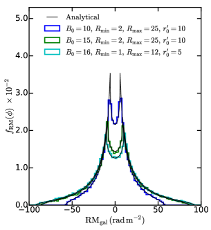
Here, $a^{\prime}=0.81\,n_{0}\,B_{0}\,h_{\rm ion}\tan i\,{\rm e}^{-R_{\rm max}/r^{\prime}_{0}}$ and $b^{\prime}=0.81\,n_{0}\,B_{0}\,h_{\rm ion}\tan i\,{\rm e}^{-R_{\rm min}/r^{\prime}_{0}}$. The left-hand panel of Fig. 1 shows the analytical PDF of ${\rm RM_{gal}}$ for a single galaxy with $i=30^{\circ}$ (black curve) and, for comparison, the simulated distribution for 10 000 lines of sight as histograms.

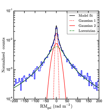
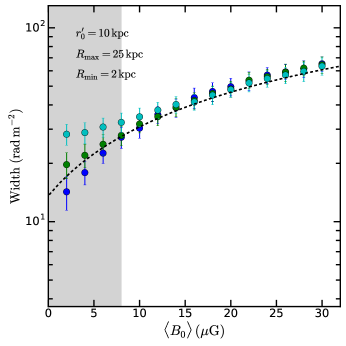
The right-hand panel of Fig. 1 shows a simulated PDF of ${\rm RM_{gal}}$ for a sample of 10 000 intervening disc galaxies, where we have assumed Gaussian distributions for $B_{0}$ (with mean $\langle B_{0}\rangle$ and standard deviation $\sigma_{B_{0}}$) and $n_{0}$ (with mean $\langle n_{0}\rangle$ and standard deviation $\sigma_{n_{\rm e}}$) within the population. We find that the distribution of ${\rm RM_{gal}}$ can be accurately approximated by the sum of one Lorentzian and two Gaussian components as shown in the right panel of Fig. 1. From Eq. (4) and Fig. 1 (left panel), we find that the width of the PDF of ${\rm RM_{gal}}$ for a single galaxy depends on the parameters $a^{\prime}$ and $b^{\prime}$ and, therefore, on $B_{0}$. Thus, we expect that the width $w$ of the Lorentzian component to be related to $\langle B_{0}\rangle$ for a sample of intervening galaxies. In Fig. 2, we show the variation of $w$ with $\langle B_{0}\rangle$ for various choices of $\sigma_{B_{0}}$. In the regime $B_{0}\gtrsim\sigma_{B_{0}}$ (the un-shaded area in Fig. 2), the variation of $w$ is approximated by,

$$w(\langle B_{0}\rangle)=13.6+1.8\,\langle B_{0}\rangle-0.0076\,\langle B_{0}\rangle^{2},$$ (5)

with $\langle B_{0}\rangle$ in $\mu$G and $w$ in rad m^-2, and is shown as the dashed line in Fig. 2. Thus, $w$ can be used to determine the mean strength of the large-scale magnetic field in a sample of intervening galaxies.

Figure 2: Variation of the width of the Lorentzian component of the distribution of ${\rm RM_{gal}}$ in the target sample as a function of $\langle B_{0}\rangle$. Blue, green and cyan symbols are for $\sigma_{B_{0}}=2,\,5\,{\rm and}\,10\,\mu$G. The dashed line is the best-fit model given by Eq. (5). The shaded region roughly represents the region where $\langle B_{0}\rangle\lesssim\sigma_{B_{0}}$ and the points within were excluded from the fitting.

4 Conclusion

Our study suggests that the distribution of ${\rm RM_{gal}}$ due to axisymmetric large-scale magnetic fields in intervening disc galaxies is non-Gaussian and that the distribution can be empirically modelled as the sum of one Lorentzian and two Gaussian components. The width of the Lorentzian component can be used to estimate the mean large-scale magnetic field strength in a population of intervening galaxies using Eq. (5) derived for typical values of the physical parameters, such as, $h_{\rm ion}=500$ pc, $R_{\rm min}=2$ kpc, $R_{\rm max}=25$ kpc and $r_{0}^{\prime}=10$ kpc. The $\langle B_{0}\rangle$ estimated using Eq. (5) lies within $\sim 50\%$ of the true value in the absence of additional constraints on the physical parameters.

References

- Basu et al. (2018) Basu A., Mao S. A., Fletcher A., Kanekar N., Shukurov A., Schnitzeler D., Vacca V., Junklewitz H., 2018, MNRAS, 477, 2528
- Berkhuijsen et al. (1997) Berkhuijsen E. M., Horellou C., Krause M., Neininger N., Poezd A. D., Shukurov A., Sokoloff D. D., 1997, A&A, 318, 700
- Bernet et al. (2008) Bernet M., Miniati F., Lilly S., Kronberg P., Dessauges-Zavadsky M., 2008, Nature, 454, 302
- Bernet et al. (2013) Bernet M. L., Miniati F., Lilly S. J., 2013, ApJ, 772, L28
- Farnes et al. (2014) Farnes J. S., O’Sullivan S. P., Corrigan M. E., Gaensler B. M., 2014, ApJ, 795, 63
- Joshi & Chand (2013) Joshi R., Chand H., 2013, MNRAS, 434, 3566
- Oren & Wolfe (1995) Oren A. L., Wolfe A. M., 1995, ApJ, 445, 624