An Approximation Algorithm for
training One-Node ReLU Neural Network

Santanu S. Dey santanu.dey@isye.gatech.edu Guanyi Wang gwang93@gatech.edu Yao Xie yao.xie@isye.gatech.edu
Abstract

Training a one-node neural network with ReLU activation function (One-Node-ReLU) is a fundamental optimization problem in deep learning. In this paper, we begin with proving the NP-hardness of training One-Node-ReLU. We then present an approximation algorithm to solve One-Node-ReLU whose running time is π’ͺ​(nk)π’ͺsuperscriptπ‘›π‘˜\mathcal{O}(n^{k}) where n𝑛n is the number of samples, kπ‘˜k is a predefined integral constant. Except kπ‘˜k, this algorithm does not require pre-processing or tuning of parameters. We analyze the performance of this algorithm under various regimes. First, given any arbitrary set of training sample data set, we show that the algorithm guarantees a nkπ‘›π‘˜\frac{n}{k}-approximation for training One-Node-ReLU problem. As a consequence, in the realizable case (i.e. when the training error is zero), this approximation algorithm achieves the global optimal solution for the One-Node-ReLU problem. Second, we assume that the training sample data is obtained from an underlying one-node neural network with ReLU activation function, where the output is perturbed by a Gaussian noise. In this regime, we show that the same approximation algorithm guarantees a much better asymptotic approximation ratio which is independent of the number of samples n𝑛n. Finally, we conduct extensive empirical studies and arrive at two conclusions. One, the approximation algorithm together with some heuristic performs better than gradient descent algorithm. Two, the solution of the approximation algorithm can be used as starting point for gradient descent – a combination that works significantly better than gradient descent.

1 Introduction

Training neural networks is a fundamental problem in machine learning.

As a first step of understanding the theoretical properties of training neural networks, we study training the most basic neural network with the following structure: a single node with rectified linear unit function (ReLU) as its activation function (See Figure 1).

[Xi]1subscriptdelimited-[]subscript𝑋𝑖1[X_{i}]_{1}[Xi]2subscriptdelimited-[]subscript𝑋𝑖2[X_{i}]_{2}[Xi]3subscriptdelimited-[]subscript𝑋𝑖3[X_{i}]_{3}[Xi]psubscriptdelimited-[]subscript𝑋𝑖𝑝[X_{i}]_{p}……\dots

ReLU

Figure 1: Single node neural network with ReLU activate function

Formally, in this paper, training a single-node neural network with ReLU activation function is the following: Given a set of n𝑛n sample points {(Xi,Yi)}i=1nβˆˆβ„p×ℝsuperscriptsubscriptsubscript𝑋𝑖subscriptπ‘Œπ‘–π‘–1𝑛superscriptℝ𝑝ℝ\{(X_{i},Y_{i})\}_{i=1}^{n}\in\mathbb{R}^{p}\times\mathbb{R} where Xisubscript𝑋𝑖X_{i} is the ithsuperscript𝑖thi^{\text{th}} input sample (observation sample), and Yisubscriptπ‘Œπ‘–Y_{i} is the ithsuperscript𝑖thi^{\text{th}} output sample (response sample), the task is to minimize the empirical average of sum of square loss

min(Ξ²,Ξ²0)βˆˆβ„p×ℝ⁑1n​‖max⁑{𝟎,XβŠ€β€‹Ξ²+Ξ²0β€‹πŸ}βˆ’Yβ€–22subscript𝛽subscript𝛽0superscriptℝ𝑝ℝ1𝑛superscriptsubscriptnorm0superscript𝑋top𝛽subscript𝛽01π‘Œ22\displaystyle\min_{(\beta,\beta_{0})\in\mathbb{R}^{p}\times\mathbb{R}}\frac{1}{n}\|\max\{\mathbf{0},X^{\top}\beta+\beta_{0}\mathbf{1}\}-Y\|_{2}^{2} (One-Node-ReLU)

where X=(X1​|X2|​…|Xn)βˆˆβ„pΓ—n𝑋conditionalsubscript𝑋1subscript𝑋2…subscript𝑋𝑛superscriptℝ𝑝𝑛X=(X_{1}|X_{2}|\ldots|X_{n})\in\mathbb{R}^{p\times n} and Y=(Yi)i=1nβˆˆβ„nΓ—1π‘Œsuperscriptsubscriptsubscriptπ‘Œπ‘–π‘–1𝑛superscriptℝ𝑛1Y=(Y_{i})_{i=1}^{n}\in\mathbb{R}^{n\times 1}.

Note that One-Node-ReLU can be viewed as a non-linear regression problem. More general versions of this problem from the perspective of nonlinear regression have been studied inΒ [18, 13], which approach this problem from a perspective of Integer programming model and heuristics.

We caution the reader that in the field of machine learning, the phrase complexity of training a neural network has been used to refer to various different problems with corresponding goals. For example, in [7], their target is to find a feasible hypothesis hβ„Žh that satisfies the false-positive rate condition and the expected loss condition. In Β [17], complexity is measured by the number of samples that is needed to learn a certain class of function. Thus, any other hardness/lower bounds depends on how the training problem is defined. We reiterate here: this paper solely deals with the computational complexity (i.e. the amount of computational effort needed and the related questions of design of algorithm) questions related to solving the optimization problemΒ One-Node-ReLU.

Note that in One-Node-ReLU problem, we do not assume Yi>0subscriptπ‘Œπ‘–0Y_{i}>0 holds for every i∈[n]𝑖delimited-[]𝑛i\in[n]. Under this formulation, if there exists i𝑖i such that Yi<0subscriptπ‘Œπ‘–0Y_{i}<0, then the optimal objective function cannot be 00. Without loss of generality, we may assume I+:={i∈[n]:Yi>0}={1,…,m}assignsuperscript𝐼conditional-set𝑖delimited-[]𝑛subscriptπ‘Œπ‘–01β€¦π‘šI^{+}:=\{i\in[n]:Y_{i}>0\}=\{1,\ldots,m\} and Iβˆ’:={i∈[n]:Yi≀0}={m+1,…,n}assignsuperscript𝐼conditional-set𝑖delimited-[]𝑛subscriptπ‘Œπ‘–0π‘š1…𝑛I^{-}:=\{i\in[n]:Y_{i}\leq 0\}=\{m+1,\ldots,n\}.

The rest of the paper is organized as follows: SectionΒ 2 presents our theoretical results and highlights comparison with related results in the literature. SectionΒ 3 presents out computational results. In SectionΒ 4, we provide concluding results. SectionΒ 5 contains all the proofs of results presented in SectionΒ 2.

2 Main Theoretical Results

Training a one-node neural network as defined in One-Node-ReLU is a non-convex optimization problem which we expect it to be challenging to solve. However, not all non-convex problems are difficult (i.e. NP-hard). For example the classical principal component analysis problem which is non-convex but can be solved in polynomial-time.

In this paper, we analyze the optimization problem One-Node-ReLU in two scenarios:

  1. 1.

    Arbitrary data: In this case, we do not assume anything about the data, i.e., the training data is arbitrary. We would like to find optimal values of Ξ²,Ξ²0𝛽subscript𝛽0\beta,\beta_{0} to fit the function max​{0,xβŠ€β€‹Ξ²+Ξ²0}max0superscriptπ‘₯top𝛽subscript𝛽0\textup{max}\{0,x^{\top}\beta+\beta_{0}\} to the given data. We would like to answer the following questions: Is this problem NP-hard? Can we come up with an approximation algorithm? How well does this approximation algorithm perform in the worst case?

  2. 2.

    Underlying statistical model: In this case, we assume that the training data is of the form: (1) Xisubscript𝑋𝑖X_{i}’s are iid sampled from a β€œreasonable” distributions, (2) Yi=max​{0,XiβŠ€β€‹Ξ²βˆ—+Ξ²0βˆ—}+Ο΅subscriptπ‘Œπ‘–max0superscriptsubscript𝑋𝑖topsuperscriptπ›½βˆ—superscriptsubscript𝛽0βˆ—italic-Ο΅Y_{i}=\textup{max}\{0,X_{i}^{\top}\beta^{\ast}+\beta_{0}^{\ast}\}+\epsilon where Ο΅italic-Ο΅\epsilon is a Gaussian noise and (Ξ²βˆ—,Ξ²0βˆ—)superscript𝛽subscriptsuperscript𝛽0(\beta^{*},\beta^{*}_{0}) is the ground truth. We show that the same approximation algorithm described for arbitrary data case above, performs significantly better.

2.1 Training One-Node-ReLU With Arbitrary Data

For the first scenario, suppose the set of sample points {(Xi,Yi)}i=1nsuperscriptsubscriptsubscript𝑋𝑖subscriptπ‘Œπ‘–π‘–1𝑛\{(X_{i},Y_{i})\}_{i=1}^{n} are fixed and arbitrary, we study One-Node-ReLU in the perspective of computational complexity. In this section, for convenience we drop the 1n1𝑛\frac{1}{n} term from the objective function from One-Node-ReLU since it does not change the optimal solution.

Our first result formalizes the fact that we expect One-Node-ReLU to be NP-hard.

Theorem 1 (NP-hardness).

The One-Node-ReLU problem is NP-hard.

See SectionΒ 5.2 for a proof. Our proof of Theorem 1 is by showing that subset sum problem can be reduced to One-Node-ReLU problem.

Comparison with related results from literature:

We study training ReLU neural networks in the perspective of NP-hardness when the input data are fixed and given. The two-layer (k+1)π‘˜1(k+1) nodes neural network problem with ReLU as activation function has been studied in [2], which shows that the training problem is NP-hard. Comparing to our main results, we show that even a more simplified structure, a neural network with one node is NP-hard. In [14], P. Manurangsi and D. Reichman independently gave another NP-hardness reduction.

Based on NP-hardness result in TheoremΒ 1, it is natural to consider an efficient approximation algorithm with multiplicative bound. We first introduce some basic notions that explain the design of the algorithm. First, we can represent the One-Node-ReLU problem by dividing the summation into two parts:

min(Ξ²,Ξ²0)βˆˆβ„p×ℝ⁑‖max⁑{𝟎,XβŠ€β€‹Ξ²+Ξ²0β€‹πŸ}βˆ’Yβ€–22subscript𝛽subscript𝛽0superscriptℝ𝑝ℝsuperscriptsubscriptnorm0superscript𝑋top𝛽subscript𝛽01π‘Œ22\displaystyle\min_{(\beta,\beta_{0})\in\mathbb{R}^{p}\times\mathbb{R}}\|\max\{\mathbf{0},X^{\top}\beta+\beta_{0}\mathbf{1}\}-Y\|_{2}^{2}
=\displaystyle= min(Ξ²,Ξ²0)βˆˆβ„pΓ—β„β€‹βˆ‘i∈{1,…,m}(max⁑{0,XiβŠ€β€‹Ξ²+Ξ²0}βˆ’Yi)2+ϕ​(Ξ²,Ξ²0)subscript𝛽subscript𝛽0superscriptℝ𝑝ℝsubscript𝑖1β€¦π‘šsuperscript0superscriptsubscript𝑋𝑖top𝛽subscript𝛽0subscriptπ‘Œπ‘–2italic-ϕ𝛽subscript𝛽0\displaystyle\min_{(\beta,\beta_{0})\in\mathbb{R}^{p}\times\mathbb{R}}\sum_{i\in\{1,\ldots,m\}}(\max\{0,X_{i}^{\top}\beta+\beta_{0}\}-Y_{i})^{2}+\phi(\beta,\beta_{0}) (βˆ—βˆ—\ast)

where ϕ​(Ξ²,Ξ²0)β‰œβˆ‘i∈{m+1,…,n}(max⁑{0,XiβŠ€β€‹Ξ²+Ξ²0}βˆ’Yi)2β‰œitalic-ϕ𝛽subscript𝛽0subscriptπ‘–π‘š1…𝑛superscript0superscriptsubscript𝑋𝑖top𝛽subscript𝛽0subscriptπ‘Œπ‘–2\phi(\beta,\beta_{0})\triangleq\sum_{i\in\{m+1,\ldots,n\}}(\max\{0,X_{i}^{\top}\beta+\beta_{0}\}-Y_{i})^{2}. It is easy to observe that:

Proposition 1.

The second term of (βˆ—italic-βˆ—\ast β€£ 2.1), that is the function ϕ​(Ξ²,Ξ²0)italic-ϕ𝛽subscript𝛽0\phi(\beta,\beta_{0}), is convex.

The first term of (βˆ—βˆ—\ast β€£ 2.1) can be further represented as a two-phase optimization problem as follows:

min(Ξ²,Ξ²0)βˆˆβ„p×ℝ⁑‖max⁑{𝟎,XβŠ€β€‹Ξ²+Ξ²0β€‹πŸ}βˆ’Yβ€–22=(minIβŠ†[m]⁑(min(Ξ²,Ξ²0)∈P​(I)⁑fI​(Ξ²,Ξ²0)))+ϕ​(Ξ²,Ξ²0)subscript𝛽subscript𝛽0superscriptℝ𝑝ℝsuperscriptsubscriptnorm0superscript𝑋top𝛽subscript𝛽01π‘Œ22subscript𝐼delimited-[]π‘šsubscript𝛽subscript𝛽0𝑃𝐼subscript𝑓𝐼𝛽subscript𝛽0italic-ϕ𝛽subscript𝛽0\displaystyle\min_{(\beta,\beta_{0})\in\mathbb{R}^{p}\times\mathbb{R}}\|\max\{\mathbf{0},X^{\top}\beta+\beta_{0}\mathbf{1}\}-Y\|_{2}^{2}=\left(\min_{I\subseteq[m]}\left(\min_{(\beta,\beta_{0})\in P(I)}f_{I}(\beta,\beta_{0})\right)\right)+\phi(\beta,\beta_{0})

where, for a given index set I𝐼I, define set P​(I)𝑃𝐼P(I) and function fI​(Ξ²,Ξ²0)subscript𝑓𝐼𝛽subscript𝛽0f_{I}(\beta,\beta_{0}) be:

P​(I):=assign𝑃𝐼absent\displaystyle P(I):= {(Ξ²,Ξ²0):XiβŠ€β€‹Ξ²+Ξ²0>0,i∈IXiβŠ€β€‹Ξ²+Ξ²0≀0,i∈[m]\I},\displaystyle\leavevmode\nobreak\ \left\{(\beta,\beta_{0}):\begin{array}[]{lll}X_{i}^{\top}\beta+\beta_{0}>0,&i\in I\\ X_{i}^{\top}\beta+\beta_{0}\leq 0,&i\in[m]\backslash I\end{array}\right\}, set of feasible region of β𝛽\beta,
fI​(Ξ²,Ξ²0):=assignsubscript𝑓𝐼𝛽subscript𝛽0absent\displaystyle f_{I}(\beta,\beta_{0}):= βˆ‘i∈I(XiβŠ€β€‹Ξ²+Ξ²0βˆ’Yi)2+βˆ‘i∈[m]\IYi2,subscript𝑖𝐼superscriptsuperscriptsubscript𝑋𝑖top𝛽subscript𝛽0subscriptπ‘Œπ‘–2subscript𝑖\delimited-[]π‘šπΌsuperscriptsubscriptπ‘Œπ‘–2\displaystyle\leavevmode\nobreak\ \sum_{i\in I}(X_{i}^{\top}\beta+\beta_{0}-Y_{i})^{2}+\sum_{i\in[m]\backslash I}Y_{i}^{2}, summation of i∈[m]𝑖delimited-[]π‘ši\in[m] via P​(I)𝑃𝐼P(I).

Henceforth, we denote the index set I𝐼I be the active set and denote the index set IC=[m]\Isuperscript𝐼𝐢\delimited-[]π‘šπΌI^{C}=[m]\backslash I be the inactive set. Hence the original One-Node-ReLU problem can be interpreted as a two-phase optimization problem: For any given IβŠ†[m]𝐼delimited-[]π‘šI\subseteq[m], the inner-phase optimization problem

zβˆ—β€‹(I):=min(Ξ²,Ξ²0)∈P​(I)⁑fI​(Ξ²,Ξ²0)+ϕ​(Ξ²,Ξ²0)assignsuperscriptπ‘§βˆ—πΌsubscript𝛽subscript𝛽0𝑃𝐼subscript𝑓𝐼𝛽subscript𝛽0italic-ϕ𝛽subscript𝛽0\displaystyle z^{\ast}(I):=\min_{(\beta,\beta_{0})\in P(I)}f_{I}(\beta,\beta_{0})+\phi(\beta,\beta_{0})

is convex over (Ξ²,Ξ²0)𝛽subscript𝛽0(\beta,\beta_{0}). the Our approximation algorithm will be build based on the fact that we will examine only a polynomial number of distinct I𝐼I’s.

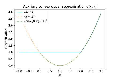
In order to obtain the approximation guarantees it is convenient to work with an β€˜unconstrained version’ of the optimization problem corresponding to zβˆ—β€‹(I)superscript𝑧𝐼z^{*}(I). Let Οƒ:ℝ×ℝ↦ℝ:𝜎maps-toℝℝℝ\sigma:\mathbb{R}\times\mathbb{R}\mapsto\mathbb{R} be the convex function (See Figure 2) defined as:
σ​(x,y)={(xβˆ’y)2Β if ​x>2​yy2Β if ​x≀2​y,𝜎π‘₯𝑦casessuperscriptπ‘₯𝑦2Β ifΒ π‘₯2𝑦missing-subexpressionsuperscript𝑦2Β ifΒ π‘₯2𝑦missing-subexpression\displaystyle\sigma(x,y)=\left\{\begin{array}[]{lll}(x-y)^{2}&\text{ if }x>2y\\ y^{2}&\text{ if }x\leq 2y,\end{array}\right.
Refer to caption
Figure 2: Function σ​(x,y)𝜎π‘₯𝑦\sigma(x,y) with y=1𝑦1y=1

where σ​(XiβŠ€β€‹Ξ²+Ξ²0,Yi)β‰₯(max⁑{0,XiβŠ€β€‹Ξ²+Ξ²0}βˆ’Yi)2𝜎superscriptsubscript𝑋𝑖top𝛽subscript𝛽0subscriptπ‘Œπ‘–superscript0superscriptsubscript𝑋𝑖top𝛽subscript𝛽0subscriptπ‘Œπ‘–2\sigma(X_{i}^{\top}\beta+\beta_{0},Y_{i})\geq(\max\{0,X_{i}^{\top}\beta+\beta_{0}\}-Y_{i})^{2} holds for all (Ξ²,Ξ²0)βˆˆβ„p×ℝ𝛽subscript𝛽0superscriptℝ𝑝ℝ(\beta,\beta_{0})\in\mathbb{R}^{p}\times\mathbb{R}. Let

zσ​(I):=min(Ξ²,Ξ²0)βˆˆβ„pΓ—β„β€‹βˆ‘i∈I(XiβŠ€β€‹Ξ²+Ξ²0βˆ’Yi)2+βˆ‘i∈[m]\Iσ​(XiβŠ€β€‹Ξ²+Ξ²0,Yi)+ϕ​(Ξ²,Ξ²0)assignsuperscriptπ‘§πœŽπΌsubscript𝛽subscript𝛽0superscriptℝ𝑝ℝsubscript𝑖𝐼superscriptsuperscriptsubscript𝑋𝑖top𝛽subscript𝛽0subscriptπ‘Œπ‘–2subscript𝑖\delimited-[]π‘šπΌπœŽsuperscriptsubscript𝑋𝑖top𝛽subscript𝛽0subscriptπ‘Œπ‘–italic-ϕ𝛽subscript𝛽0\displaystyle z^{\sigma}(I):=\min_{(\beta,\beta_{0})\in\mathbb{R}^{p}\times\mathbb{R}}{\sum_{i\in I}(X_{i}^{\top}\beta+\beta_{0}-Y_{i})^{2}+\sum_{i\in[m]\backslash I}\sigma(X_{i}^{\top}\beta+\beta_{0},Y_{i})}+\phi(\beta,\beta_{0})

be an convex upper approximation of zβˆ—β€‹(I)superscriptπ‘§βˆ—πΌz^{\ast}(I). Let

zOPTsuperscript𝑧OPT\displaystyle z^{\text{OPT}} :=min(Ξ²,Ξ²0)βˆˆβ„p×ℝ⁑‖max⁑{𝟎,XβŠ€β€‹Ξ²+Ξ²0β€‹πŸ}βˆ’Yβ€–22,assignabsentsubscript𝛽subscript𝛽0superscriptℝ𝑝ℝsuperscriptsubscriptnorm0superscript𝑋top𝛽subscript𝛽01π‘Œ22\displaystyle:=\min_{(\beta,\beta_{0})\in\mathbb{R}^{p}\times\mathbb{R}}\|\max\{\mathbf{0},X^{\top}\beta+\beta_{0}\mathbf{1}\}-Y\|_{2}^{2}, be the global optimal value,
(Ξ²OPT,Ξ²0OPT)superscript𝛽OPTsubscriptsuperscript𝛽OPT0\displaystyle(\beta^{\text{OPT}},\beta^{\text{OPT}}_{0}) :=arg​min(Ξ²,Ξ²0)βˆˆβ„p×ℝ⁑‖max⁑{𝟎,XβŠ€β€‹Ξ²+Ξ²0β€‹πŸ}βˆ’Yβ€–22,assignabsentsubscriptargmin𝛽subscript𝛽0superscriptℝ𝑝ℝsuperscriptsubscriptnorm0superscript𝑋top𝛽subscript𝛽01π‘Œ22\displaystyle:=\operatorname*{arg\,min}_{(\beta,\beta_{0})\in\mathbb{R}^{p}\times\mathbb{R}}\|\max\{\mathbf{0},X^{\top}\beta+\beta_{0}\mathbf{1}\}-Y\|_{2}^{2}, be a global optimal solution.

Thus IOPT:={i∈[m]:XiβŠ€β€‹Ξ²OPT+Ξ²0OPT>0}assignsuperscript𝐼OPTconditional-set𝑖delimited-[]π‘šsuperscriptsubscript𝑋𝑖topsuperscript𝛽OPTsubscriptsuperscript𝛽OPT00I^{\text{OPT}}:=\left\{i\in[m]:X_{i}^{\top}\beta^{\text{OPT}}+\beta^{\text{OPT}}_{0}>0\right\} and [m]\IOPT:={i∈[m]:XiβŠ€β€‹Ξ²OPT+Ξ²0OPT≀0}assign\delimited-[]π‘šsuperscript𝐼OPTconditional-set𝑖delimited-[]π‘šsuperscriptsubscript𝑋𝑖topsuperscript𝛽OPTsubscriptsuperscript𝛽OPT00[m]\backslash I^{\text{OPT}}:=\left\{i\in[m]:X_{i}^{\top}\beta^{\text{OPT}}+\beta^{\text{OPT}}_{0}\leq 0\right\} are the corresponding active, inactive set of (Ξ²OPT,Ξ²0OPT)superscript𝛽OPTsubscriptsuperscript𝛽OPT0(\beta^{\text{OPT}},\beta^{\text{OPT}}_{0}) respectively. Then zσ​(I)superscriptπ‘§πœŽπΌz^{\sigma}(I) satisfies:

Proposition 2.

For any IβŠ†[m]𝐼delimited-[]π‘šI\subseteq[m], zOPT≀zσ​(I)superscript𝑧OPTsuperscriptπ‘§πœŽπΌz^{\text{OPT}}\leq z^{\sigma}(I). Moreover, there exists a IβŠ†[m]𝐼delimited-[]π‘šI\subseteq[m] such that zOPT=zσ​(I)superscript𝑧OPTsuperscriptπ‘§πœŽπΌz^{\text{OPT}}=z^{\sigma}(I).

Proof of Proposition 2 can be found in Section 5.3. Thus, we can use the zσ​(I)superscriptπ‘§πœŽπΌz^{\sigma}(I) functions instead of zβˆ—β€‹(I)superscript𝑧𝐼z^{*}(I) to design the algorithm, and being an unconstrained problem is easier to work with.

Given any feasible solution (Ξ²,Ξ²0)𝛽subscript𝛽0(\beta,\beta_{0}), by definition, the ithsuperscript𝑖thi^{\text{th}} row will contribute

(max⁑{0,XiβŠ€β€‹Ξ²+Ξ²0}βˆ’Yi)2superscript0superscriptsubscript𝑋𝑖top𝛽subscript𝛽0subscriptπ‘Œπ‘–2\displaystyle\left(\max\{0,X_{i}^{\top}\beta+\beta_{0}\}-Y_{i}\right)^{2}

to the objective value. Suppose the given (Ξ²,Ξ²0)𝛽subscript𝛽0(\beta,\beta_{0}) satisfies

XiβŠ€β€‹Ξ²+Ξ²0≀0,superscriptsubscript𝑋𝑖top𝛽subscript𝛽00\displaystyle X_{i}^{\top}\beta+\beta_{0}\leq 0,

then for some i∈[m]𝑖delimited-[]π‘ši\in[m] such that 0β‰ͺYimuch-less-than0subscriptπ‘Œπ‘–0\ll Y_{i}, the ithsuperscript𝑖thi^{\text{th}} row contributes a large value to objective. Therefore, we expect the greater Yisubscriptπ‘Œπ‘–Y_{i}, the more likely that the index i𝑖i is in the active set. This is the key intuition behind AlgorithmΒ 1, which explores a polynomial number of active sets with the property that larger the value of Yisubscriptπ‘Œπ‘–Y_{i} the more likely i𝑖i is in the active set.

Algorithm 1 Generalized Approximation Algorithm
1:Input: A set of n𝑛n sample points (X,Y)βˆˆβ„pΓ—n×ℝnπ‘‹π‘Œsuperscriptℝ𝑝𝑛superscriptℝ𝑛(X,Y)\in\mathbb{R}^{p\times n}\times\mathbb{R}^{n}, a positive-label index set I+={1,…,m}superscript𝐼1β€¦π‘šI^{+}=\{1,\ldots,m\} such that 0<Y1≀Y2≀⋯≀Ym0subscriptπ‘Œ1subscriptπ‘Œ2β‹―subscriptπ‘Œπ‘š0<Y_{1}\leq Y_{2}\leq\dots\leq Y_{m}, a negative-label index set Iβˆ’={m+1,…,n}superscriptπΌπ‘š1…𝑛I^{-}=\{m+1,\ldots,n\}, a fixed integer kβ‰₯1π‘˜1k\geq 1.
2:Output: A feasible n/kπ‘›π‘˜n/k-approximation solution (Ξ²,Ξ²0)𝛽subscript𝛽0(\beta,\beta_{0}) for the One-Node-ReLU problem.
3:functionΒ Generalized Approximation Algorithm(X,Y,I+π‘‹π‘Œsuperscript𝐼X,Y,I^{+})
4:Β Β Β Β Β forΒ j=1,…,k𝑗1β€¦π‘˜j=1,\ldots,k as the size of inactive set [m]\I\delimited-[]π‘šπΌ[m]\backslash IΒ do
5:Β Β Β Β Β Β Β Β Β Pick j𝑗j distinct indices i1,…,ijsubscript𝑖1…subscript𝑖𝑗i_{1},\ldots,i_{j} such that 0≀i1<…<ij≀m0subscript𝑖1…subscriptπ‘–π‘—π‘š0\leq i_{1}<\ldots<i_{j}\leq m.
6:Β Β Β Β Β Β Β Β Β Set inactive set be
{{1,…,i1}βˆͺ(⋃ℓ=2j{iβ„“})Β for ​jβ‰₯2,{1,…,i1}Β for ​j=1.cases1…subscript𝑖1superscriptsubscriptβ„“2𝑗subscript𝑖ℓ for 𝑗2missing-subexpression1…subscript𝑖1Β for 𝑗1missing-subexpression\displaystyle\left\{\begin{array}[]{lll}\left\{1,\ldots,i_{1}\right\}\cup\left(\bigcup_{\ell=2}^{j}\{i_{\ell}\}\right)&\text{ for }j\geq 2,\\ \left\{1,\ldots,i_{1}\right\}&\text{ for }j=1.\end{array}\right.
7:Β Β Β Β Β Β Β Β Β Set active set be the complement of inactive set as
I=(⋃ℓ=1jβˆ’1{iβ„“+1,…,iβ„“+1βˆ’1})βˆͺ{ij+1,…,m}.𝐼superscriptsubscriptβ„“1𝑗1subscript𝑖ℓ1…subscript𝑖ℓ11subscript𝑖𝑗1β€¦π‘š\displaystyle I=\left(\bigcup_{\ell=1}^{j-1}\left\{i_{\ell}+1,\ldots,i_{\ell+1}-1\right\}\right)\cup\{i_{j}+1,\ldots,m\}.
8:         For each active set I𝐼I, compute
(Ξ²I,Ξ²0I)←←superscript𝛽𝐼subscriptsuperscript𝛽𝐼0absent\displaystyle(\beta^{I},\beta^{I}_{0})\leftarrow arg​min(Ξ²,Ξ²0)⁑fIσ​(Ξ²,Ξ²0)+ϕ​(Ξ²,Ξ²0),subscriptargmin𝛽subscript𝛽0subscriptsuperscriptπ‘“πœŽπΌπ›½subscript𝛽0italic-ϕ𝛽subscript𝛽0\displaystyle\operatorname*{arg\,min}_{(\beta,\beta_{0})}f^{\sigma}_{I}(\beta,\beta_{0})+\phi(\beta,\beta_{0}),
zσ​(I)←←superscriptπ‘§πœŽπΌabsent\displaystyle z^{\sigma}(I)\leftarrow min(Ξ²,Ξ²0)⁑fIσ​(Ξ²,Ξ²0)+ϕ​(Ξ²,Ξ²0).subscript𝛽subscript𝛽0subscriptsuperscriptπ‘“πœŽπΌπ›½subscript𝛽0italic-ϕ𝛽subscript𝛽0\displaystyle\min_{(\beta,\beta_{0})}f^{\sigma}_{I}(\beta,\beta_{0})+\phi(\beta,\beta_{0}).
Β Β Β Β Β 
9:Β Β Β Β Β return (Ξ²^,Ξ²^0)^𝛽subscript^𝛽0(\hat{\beta},\hat{\beta}_{0}) which corresponds to the minimum zσ​(I)superscriptπ‘§πœŽπΌz^{\sigma}(I) among all the I𝐼I’s examined.

Note that when i1=0subscript𝑖10i_{1}=0, the set {1,…,i1}=βˆ…1…subscript𝑖1\{1,\ldots,i_{1}\}=\emptyset, similarly, when ij=msubscriptπ‘–π‘—π‘ši_{j}=m, the set {ik+1,…,m}=βˆ…subscriptπ‘–π‘˜1β€¦π‘š\{i_{k}+1,\ldots,m\}=\emptyset. It is clear to see that, for each j=1,…,k𝑗1β€¦π‘˜j=1,\ldots,k, there are (mj)binomialπ‘šπ‘—\binom{m}{j} distinct subsets {i1,…,ij}subscript𝑖1…subscript𝑖𝑗\{i_{1},\ldots,i_{j}\} in {1,…,m}1β€¦π‘š\{1,\ldots,m\}. For each subset {i1,…,ij}subscript𝑖1…subscript𝑖𝑗\{i_{1},\ldots,i_{j}\}, Algorithm 1 requires to solve a convex optimization problem, thus the total running time of Algorithm 1 is

(βˆ‘i=1k(ni))​T=O​(nk​T)superscriptsubscript𝑖1π‘˜binomial𝑛𝑖𝑇𝑂superscriptπ‘›π‘˜π‘‡\left(\sum_{i=1}^{k}\binom{n}{i}\right)T=O\left(n^{k}T\right)

where T𝑇T is the running time of solving a convex optimization problem

(Ξ²I,Ξ²0I)←arg​min(Ξ²,Ξ²0)⁑fIσ​(Ξ²,Ξ²0)+ϕ​(Ξ²,Ξ²0).←superscript𝛽𝐼subscriptsuperscript𝛽𝐼0subscriptargmin𝛽subscript𝛽0subscriptsuperscriptπ‘“πœŽπΌπ›½subscript𝛽0italic-ϕ𝛽subscript𝛽0(\beta^{I},\beta^{I}_{0})\leftarrow\operatorname*{arg\,min}_{(\beta,\beta_{0})}f^{\sigma}_{I}(\beta,\beta_{0})+\phi(\beta,\beta_{0}).

Thus Algorithm 1 is a polynomial-time algorithm.

Theorem 2 (Approximation Ratio).

AlgorithmΒ 1 is an nkπ‘›π‘˜\frac{n}{k}-Approximation Algorithm, i.e., if za​p​p​r​o​xsuperscriptπ‘§π‘Žπ‘π‘π‘Ÿπ‘œπ‘₯z^{approx} is the objective value of the (Ξ²^,Ξ²0^)^𝛽^subscript𝛽0(\hat{\beta},\hat{\beta_{0}}) returned from AlgorithmΒ 1, and zOPTsuperscript𝑧OPTz^{\text{OPT}} is the global optimal value of One-Node-ReLU, then:

zOPT≀za​p​p​r​o​x≀nk​zOPT.superscript𝑧OPTsuperscriptπ‘§π‘Žπ‘π‘π‘Ÿπ‘œπ‘₯π‘›π‘˜superscript𝑧OPTz^{\text{OPT}}\leq z^{approx}\leq\frac{n}{k}z^{\text{OPT}}.
Comparison with related results from literature:

Note that there is an exact algorithm that solves One-Node-ReLU problem within O​(np)𝑂superscript𝑛𝑝O(n^{p}) running time where p𝑝p is the dimensionΒ [1]. However, when p𝑝p is much greater than n𝑛n (i.e., in high dimensional cases), our generalized approximation algorithm could achieve a reasonable good solution in O​(nk​T)𝑂superscriptπ‘›π‘˜π‘‡O(n^{k}T) running time. In [14], P. Manurangsi and D. Reichman show that minimizing squared training error of a one-node neural network is NP-hard to approximate within the factor n1(log⁑log⁑n)O​(1)superscript𝑛1superscript𝑛𝑂1n^{\frac{1}{(\log\log n)^{O(1)}}} (actually, mπ‘šm samples {(xi,yi)}i=1msuperscriptsubscriptsubscriptπ‘₯𝑖subscript𝑦𝑖𝑖1π‘š\{(x_{i},y_{i})\}_{i=1}^{m} in their setting generates n​mπ‘›π‘šnm samples in our setting based their polynomial-time reduction). There is a significant gap between upper bound from AlgorithmΒ 1 and this lower bound.

A very important consequence of TheoremΒ 2 is the following result.

Corollary 1 (Realizable case).

When the One-Node-ReLU problem is realizable, i.e., there exists a true solution (Ξ²βˆ—,Ξ²0βˆ—)superscriptπ›½βˆ—subscriptsuperscriptπ›½βˆ—0(\beta^{\ast},\beta^{\ast}_{0}) with 0 objective value, then TheoremΒ 2 implies that the AlgorithmΒ 1 gives a polynomial-time approach that solves the One-Node-ReLU problem exactly to global optimal.

Comparison with related results in literature

Soltanolkotabi in [16], and Kalan et.al. in [12] studied the problem of learning one node ReLU neural network with i.i.d. random Gaussian distribution observation samples via gradient descent (GD) method and stochastic gradient descent (SGD) method in the realizable case. Soltanolkotabi showed that the gradient descent, when starting from origin converges at a linear rate to the true solution (with additive error) where the number of samples is sufficiently large. Kalan et.al. in [12] discussed the stochastic version that mini-batch stochastic gradient descent when suitably initialized, converges at a geometric rate to the true solution (with additive error). In contrast AlgorithmΒ 1 does not need the assumption that the data is i.i.d. random Gaussian distribution, there are no additive errors, and also deals with the case where Ξ²0subscript𝛽0\beta_{0} is non-trivial. Finally, the initialization of SGD method requires some additional effort not needed for AlgorithmΒ 1.

2.2 Training One-Node-ReLU With Underlying Statistical Model

In real life, it is natural to assume that the set of sample points follows some underlying statistical model. Here is our assumptions:

Assumption 1 (Underlying Statistical Model).

Suppose the set of sample points

(X1,Y1),…,(Xn,Yn)βˆˆβ„p×ℝsubscript𝑋1subscriptπ‘Œ1…subscript𝑋𝑛subscriptπ‘Œπ‘›superscriptℝ𝑝ℝ(X_{1},Y_{1}),\ldots,(X_{n},Y_{n})\in\mathbb{R}^{p}\times\mathbb{R}

satisfies the correct underlying statistical model, i.e., for each i=1,…,n𝑖1…𝑛i=1,\ldots,n,

Yi=max⁑{0,XiβŠ€β€‹Ξ²βˆ—+Ξ²0βˆ—}+Ο΅isubscriptπ‘Œπ‘–0superscriptsubscript𝑋𝑖topsuperscriptπ›½βˆ—subscriptsuperscriptπ›½βˆ—0subscriptitalic-ϡ𝑖\displaystyle Y_{i}=\max\{0,X_{i}^{\top}\beta^{\ast}+\beta^{\ast}_{0}\}+\epsilon_{i}

where Ξ²βˆ—,Ξ²0βˆ—superscriptπ›½βˆ—subscriptsuperscriptπ›½βˆ—0\beta^{\ast},\beta^{\ast}_{0} is some fixed true parameter (may be distinct from (Ξ²OPT,Ξ²0OPT)superscript𝛽OPTsubscriptsuperscript𝛽OPT0\left(\beta^{\text{OPT}},\beta^{\text{OPT}}_{0}\right) as the optimal solution of One-Node-ReLU). We further assume that Ξ²βˆ—,Ξ²0βˆ—superscriptπ›½βˆ—subscriptsuperscriptπ›½βˆ—0\beta^{\ast},\beta^{\ast}_{0} belongs to a convex compact set Ξ˜βŠ†β„pΓ—β„Ξ˜superscriptℝ𝑝ℝ\Theta\subseteq\mathbb{R}^{p}\times\mathbb{R}, and for i=1,…,n𝑖1…𝑛i=1,\ldots,n, Xi,Ο΅isubscript𝑋𝑖subscriptitalic-ϡ𝑖X_{i},\epsilon_{i} are i.i.d. random variables that are generated from some underlying fixed distribution 𝒩,π’Ÿπ’©π’Ÿ\mathcal{N},\mathcal{D}, respectively. Furthermore, 𝒩𝒩\mathcal{N} is a distribution that satisfies the following properties:

  1. 1.

    𝔼XβˆΌπ’©β€‹[X]=0p,Β andΒ VarXβˆΌπ’©β€‹(X)=Ξ£formulae-sequencesubscript𝔼similar-to𝑋𝒩delimited-[]𝑋subscript0𝑝subscriptΒ andΒ Varsimilar-to𝑋𝒩𝑋Σ\mathbb{E}_{X\sim\mathcal{N}}[X]=0_{p},\text{ and }\text{Var}_{X\sim\mathcal{N}}(X)=\Sigma positive semi-definite.

  2. 2.

    Unique Optimal Property: Let Suppπ’©βŠ†β„psubscriptSupp𝒩superscriptℝ𝑝\text{Supp}_{\mathcal{N}}\subseteq\mathbb{R}^{p} be the support of distribution 𝒩𝒩\mathcal{N}. For any (Ξ²βˆ—,Ξ²0βˆ—)∈Θsuperscriptπ›½βˆ—subscriptsuperscriptπ›½βˆ—0Θ(\beta^{\ast},\beta^{\ast}_{0})\in\Theta, there exists p+1𝑝1p+1 vectors v1,…,vp,vp+1∈Supp𝒩subscript𝑣1…subscript𝑣𝑝subscript𝑣𝑝1subscriptSupp𝒩v_{1},\ldots,v_{p},v_{p+1}\in\text{Supp}_{\mathcal{N}} such that

    viβŠ€β€‹Ξ²βˆ—+Ξ²0βˆ—>0,βˆ€i=1,…,p,p+1,formulae-sequencesuperscriptsubscript𝑣𝑖topsuperscriptπ›½βˆ—subscriptsuperscriptπ›½βˆ—00for-all𝑖1…𝑝𝑝1\displaystyle v_{i}^{\top}\beta^{\ast}+\beta^{\ast}_{0}>0,\leavevmode\nobreak\ \forall i=1,\ldots,p,p+1,

    in which (v1,1),…,(vp,1),(vp+1,1)βˆˆβ„p+1subscript𝑣11…subscript𝑣𝑝1subscript𝑣𝑝11superscriptℝ𝑝1(v_{1},1),\ldots,(v_{p},1),(v_{p+1},1)\in\mathbb{R}^{p+1} are linearly independent.

  3. 3.

    Since Ξ²βˆ—,Ξ²0βˆ—superscriptπ›½βˆ—subscriptsuperscriptπ›½βˆ—0\beta^{\ast},\beta^{\ast}_{0} is fixed then

    𝔼XβˆΌπ’©[XβŠ€Ξ²βˆ—+Ξ²0βˆ—]=Ξ²0βˆ—,Β andΒ VarXβˆΌπ’©(XβŠ€Ξ²βˆ—+Ξ²0βˆ—)=(Ξ²βˆ—)βŠ€Ξ£Ξ²βˆ—=:Ξ”2.\mathbb{E}_{X\sim\mathcal{N}}[X^{\top}\beta^{\ast}+\beta^{\ast}_{0}]=\beta^{\ast}_{0},\text{ and }\text{Var}_{X\sim\mathcal{N}}(X^{\top}\beta^{\ast}+\beta^{\ast}_{0})=(\beta^{\ast})^{\top}\Sigma\beta^{\ast}=:\Delta^{2}.

and π’Ÿπ’Ÿ\mathcal{D} is a Gaussian distribution such that π”ΌΟ΅βˆΌπ’Ÿ=0subscript𝔼similar-toitalic-Ο΅π’Ÿ0\mathbb{E}_{\epsilon\sim\mathcal{D}}=0 and VarΟ΅βˆΌπ’Ÿ=Ξ³2<∞subscriptVarsimilar-toitalic-Ο΅π’Ÿsuperscript𝛾2\text{Var}_{\epsilon\sim\mathcal{D}}=\gamma^{2}<\infty.

Note that AlgorithmΒ 1 with parameter k=1π‘˜1k=1, provides a solution to the objective function in the following format:

minβ∈Θ⁑1n​[βˆ‘i∈I​(y)σ​(XiβŠ€β€‹Ξ²+Ξ²0,Yi)+βˆ‘i∈I+\I​(y)(XiβŠ€β€‹Ξ²+Ξ²0βˆ’Yi)2+βˆ‘i∈Iβˆ’(max⁑{0,XiβŠ€β€‹Ξ²+Ξ²0}βˆ’Yi)2]⏟=⁣:Sny​(Ξ²,Ξ²0)subscriptπ›½Ξ˜subscript⏟1𝑛delimited-[]subscriptπ‘–πΌπ‘¦πœŽsuperscriptsubscript𝑋𝑖top𝛽subscript𝛽0subscriptπ‘Œπ‘–subscript𝑖\superscript𝐼𝐼𝑦superscriptsuperscriptsubscript𝑋𝑖top𝛽subscript𝛽0subscriptπ‘Œπ‘–2subscript𝑖superscript𝐼superscript0superscriptsubscript𝑋𝑖top𝛽subscript𝛽0subscriptπ‘Œπ‘–2:absentsubscriptsuperscript𝑆𝑦𝑛𝛽subscript𝛽0\displaystyle\min_{\beta\in\Theta}\underbrace{\frac{1}{n}\bigg{[}\sum_{i\in I(y)}\sigma(X_{i}^{\top}\beta+\beta_{0},Y_{i})+\sum_{i\in I^{+}\backslash I(y)}(X_{i}^{\top}\beta+\beta_{0}-Y_{i})^{2}+\sum_{i\in I^{-}}(\max\{0,X_{i}^{\top}\beta+\beta_{0}\}-Y_{i})^{2}\bigg{]}}_{=:S^{y}_{n}(\beta,\beta_{0})}

where I+={i:Yi>0},Iβˆ’={i:Yi≀0}formulae-sequencesuperscript𝐼conditional-set𝑖subscriptπ‘Œπ‘–0superscript𝐼conditional-set𝑖subscriptπ‘Œπ‘–0I^{+}=\{i:Y_{i}>0\},\leavevmode\nobreak\ I^{-}=\{i:Y_{i}\leq 0\}, and I​(y)={i:0<Yi≀y}𝐼𝑦conditional-set𝑖0subscriptπ‘Œπ‘–π‘¦I(y)=\{i:0<Y_{i}\leq y\} for some y>0𝑦0y>0. To see the exact correspondence: {0,1,…,i1}01…subscript𝑖1\{0,1,\dots,i_{1}\} is I​(y)𝐼𝑦I(y) and {i1+1,…,m}i_{1}+1,\dots,m\} is [m]βˆ–I​(y)delimited-[]π‘šπΌπ‘¦[m]\setminus I(y). As we change y𝑦y, we are effectively picking different values of iisubscript𝑖𝑖i_{i}.

First, using existing classical results in ([15], p40) and [10], we obtain the following results:

Proposition 3.

As nβ†’βˆžβ†’π‘›n\rightarrow\infty, the objective function Sny​(Ξ²,Ξ²0)subscriptsuperscript𝑆𝑦𝑛𝛽subscript𝛽0S^{y}_{n}(\beta,\beta_{0}) converges to the following asymptotic objective function:

Sny​(Ξ²,Ξ²0)→𝔼XβˆΌπ’©,Ο΅βˆΌπ’Ÿβ€‹[ψy​(XβŠ€β€‹Ξ²+Ξ²0,Y)],β†’subscriptsuperscript𝑆𝑦𝑛𝛽subscript𝛽0subscript𝔼formulae-sequencesimilar-to𝑋𝒩similar-toitalic-Ο΅π’Ÿdelimited-[]subscriptπœ“π‘¦superscript𝑋top𝛽subscript𝛽0π‘Œ\displaystyle S^{y}_{n}(\beta,\beta_{0})\rightarrow\mathbb{E}_{X\sim\mathcal{N},\epsilon\sim\mathcal{D}}\bigg{[}\psi_{y}(X^{\top}\beta+\beta_{0},Y)\bigg{]},

for almost every sequence {(Xi,Yi)}i=1nsuperscriptsubscriptsubscript𝑋𝑖subscriptπ‘Œπ‘–π‘–1𝑛\{(X_{i},Y_{i})\}_{i=1}^{n} where Yi=max⁑{0,XiβŠ€β€‹Ξ²βˆ—+Ξ²0βˆ—}+Ο΅isubscriptπ‘Œπ‘–0superscriptsubscript𝑋𝑖topsuperscriptπ›½βˆ—superscriptsubscript𝛽0βˆ—subscriptitalic-ϡ𝑖Y_{i}=\max\{0,X_{i}^{\top}\beta^{\ast}+\beta_{0}^{\ast}\}+\epsilon_{i} and

ψy​(XβŠ€β€‹Ξ²+Ξ²0,Y):={σ​(XβŠ€β€‹Ξ²+Ξ²0,Y)Β if ​0<Y≀y(XβŠ€β€‹Ξ²+Ξ²0βˆ’Y)2Β if ​y<Y(max⁑{0,XβŠ€β€‹Ξ²+Ξ²0}βˆ’Y)2Β if ​Y≀0.assignsubscriptπœ“π‘¦superscript𝑋top𝛽subscript𝛽0π‘Œcases𝜎superscript𝑋top𝛽subscript𝛽0π‘ŒΒ ifΒ 0π‘Œπ‘¦missing-subexpressionmissing-subexpressionsuperscriptsuperscript𝑋top𝛽subscript𝛽0π‘Œ2Β ifΒ π‘¦π‘Œmissing-subexpressionmissing-subexpressionsuperscript0superscript𝑋top𝛽subscript𝛽0π‘Œ2Β ifΒ π‘Œ0missing-subexpressionmissing-subexpression\displaystyle\psi_{y}(X^{\top}\beta+\beta_{0},Y):=\left\{\begin{array}[]{llll}\sigma(X^{\top}\beta+\beta_{0},Y)&\text{ if }0<Y\leq y\\ (X^{\top}\beta+\beta_{0}-Y)^{2}&\text{ if }y<Y\\ (\max\{0,X^{\top}\beta+\beta_{0}\}-Y)^{2}&\text{ if }Y\leq 0\end{array}\right..
Proposition 4.

Given the set of sample points {(Xi,Yi)}i=1nsuperscriptsubscriptsubscript𝑋𝑖subscriptπ‘Œπ‘–π‘–1𝑛\{(X_{i},Y_{i})\}_{i=1}^{n} from the underlying statistical model, as nβ†’βˆžβ†’π‘›n\rightarrow\infty, the least square estimator (Ξ²OPT,Ξ²0OPT)superscript𝛽OPTsubscriptsuperscript𝛽OPT0(\beta^{\text{OPT}},\beta^{\text{OPT}}_{0}) which depends on {(Xi,Yi)}i=1nsuperscriptsubscriptsubscript𝑋𝑖subscriptπ‘Œπ‘–π‘–1𝑛\{(X_{i},Y_{i})\}_{i=1}^{n} obtained from One-Node-ReLU problem converges to the true parameter (Ξ²βˆ—,Ξ²0βˆ—)superscriptπ›½βˆ—subscriptsuperscriptπ›½βˆ—0(\beta^{\ast},\beta^{\ast}_{0}) almost surely, i.e., the estimator (Ξ²OPT,Ξ²0OPT)superscript𝛽OPTsubscriptsuperscript𝛽OPT0(\beta^{\text{OPT}},\beta^{\text{OPT}}_{0}) of (Ξ²βˆ—,Ξ²0βˆ—)superscriptπ›½βˆ—subscriptsuperscriptπ›½βˆ—0(\beta^{\ast},\beta^{\ast}_{0}) is said to be strongly consistent. Moreover, as nβ†’βˆžβ†’π‘›n\rightarrow\infty,

1nβ€‹βˆ‘i=1n(max⁑{0,XiβŠ€β€‹Ξ²+Ξ²0}βˆ’Yi)2→𝔼XβˆΌπ’©,Ο΅βˆΌπ’Ÿβ€‹[(max⁑{0,XβŠ€β€‹Ξ²+Ξ²0}βˆ’Y)2],β†’1𝑛superscriptsubscript𝑖1𝑛superscript0superscriptsubscript𝑋𝑖top𝛽subscript𝛽0subscriptπ‘Œπ‘–2subscript𝔼formulae-sequencesimilar-to𝑋𝒩similar-toitalic-Ο΅π’Ÿdelimited-[]superscript0superscript𝑋top𝛽subscript𝛽0π‘Œ2\displaystyle\frac{1}{n}\sum_{i=1}^{n}\left(\max\{0,X_{i}^{\top}\beta+\beta_{0}\}-Y_{i}\right)^{2}\rightarrow\mathbb{E}_{X\sim\mathcal{N},\epsilon\sim\mathcal{D}}\left[\left(\max\{0,X^{\top}\beta+\beta_{0}\}-Y\right)^{2}\right],

and

min(Ξ²,Ξ²0)βˆˆΞ˜β‘π”ΌXβˆΌπ’©,Ο΅βˆΌπ’Ÿβ€‹[(max⁑{0,XβŠ€β€‹Ξ²+Ξ²0}βˆ’Y)2]=𝔼XβˆΌπ’©,Ο΅βˆΌπ’Ÿβ€‹[(max⁑{0,XβŠ€β€‹Ξ²βˆ—+Ξ²0βˆ—}βˆ’Y)2]=Ξ³2.subscript𝛽subscript𝛽0Θsubscript𝔼formulae-sequencesimilar-to𝑋𝒩similar-toitalic-Ο΅π’Ÿdelimited-[]superscript0superscript𝑋top𝛽subscript𝛽0π‘Œ2subscript𝔼formulae-sequencesimilar-to𝑋𝒩similar-toitalic-Ο΅π’Ÿdelimited-[]superscript0superscript𝑋topsuperscriptπ›½βˆ—subscriptsuperscriptπ›½βˆ—0π‘Œ2superscript𝛾2\displaystyle\min_{(\beta,\beta_{0})\in\Theta}\mathbb{E}_{X\sim\mathcal{N},\epsilon\sim\mathcal{D}}\left[\left(\max\{0,X^{\top}\beta+\beta_{0}\}-Y\right)^{2}\right]=\mathbb{E}_{X\sim\mathcal{N},\epsilon\sim\mathcal{D}}\left[\left(\max\{0,X^{\top}\beta^{\ast}+\beta^{\ast}_{0}\}-Y\right)^{2}\right]=\gamma^{2}.

Combining PropositionΒ 3 and PropositionΒ 4, we show in SectionΒ 5.5 that AlgorithmΒ 1 guarantees an asymptotic bound as follows:

Theorem 3 (Asymptotic Bound).

Assuming the underlying statistical modelΒ 1, let zasysuperscript𝑧asyz^{\text{asy}} be the optimal value of the asymptotic objective function 𝔼XβˆΌπ’©,Ο΅βˆΌπ’Ÿβ€‹[ψy​(XβŠ€β€‹Ξ²+Ξ²0,Y)]subscript𝔼formulae-sequencesimilar-to𝑋𝒩similar-toitalic-Ο΅π’Ÿdelimited-[]subscriptπœ“π‘¦superscript𝑋top𝛽subscript𝛽0π‘Œ\mathbb{E}_{X\sim\mathcal{N},\epsilon\sim\mathcal{D}}\left[\psi_{y}(X^{\top}\beta+\beta_{0},Y)\right] for all y>0𝑦0y>0, i.e.,

zasy=minyβ‰₯0⁑min(Ξ²,Ξ²0)βˆˆΞ˜β‘π”ΌXβˆΌπ’©,Ο΅βˆΌπ’Ÿβ€‹[ψy​(XβŠ€β€‹Ξ²+Ξ²0,Y)],superscript𝑧asysubscript𝑦0subscript𝛽subscript𝛽0Θsubscript𝔼formulae-sequencesimilar-to𝑋𝒩similar-toitalic-Ο΅π’Ÿdelimited-[]subscriptπœ“π‘¦superscript𝑋top𝛽subscript𝛽0π‘Œ\displaystyle z^{\text{asy}}=\min_{y\geq 0}\min_{(\beta,\beta_{0})\in\Theta}\mathbb{E}_{X\sim\mathcal{N},\epsilon\sim\mathcal{D}}\left[\psi_{y}(X^{\top}\beta+\beta_{0},Y)\right],

then zasysuperscript𝑧asyz^{\text{asy}} can be lower and upper bounded by the following:

Ξ³2≀zasy≀3​γ22+2+2​Δ22​π​γsuperscript𝛾2superscript𝑧asy3superscript𝛾2222superscriptΞ”22πœ‹π›Ύ\displaystyle\gamma^{2}\leq z^{\text{asy}}\leq\frac{3\gamma^{2}}{2}+\frac{2+2\Delta^{2}}{\sqrt{2\pi}}\gamma

where γ𝛾\gamma and ΔΔ\Delta are defined in the underlying statistical modelΒ 1.

Note that the upper bound for the asymptotic optimal value zasysuperscript𝑧asyz^{\text{asy}} only depends on the variance Ξ”2superscriptΞ”2\Delta^{2} and Ξ³2superscript𝛾2\gamma^{2}, therefore for any fixed underlying distribution 𝒩𝒩\mathcal{N} and π’Ÿπ’Ÿ\mathcal{D}, we have the following corollary:

Corollary 2 (Asymptotic Approximation Ratio).

Assuming the underlying statistical modelΒ 1, as nβ†’βˆžβ†’π‘›n\rightarrow\infty, the solution obtained from Approximation AlgorithmΒ 1 provides an asymptotic multiplicative approximation ratio

ρ≀32+2+2​Δ22​π​1γ𝜌3222superscriptΞ”22πœ‹1𝛾\displaystyle\rho\leq\frac{3}{2}+\frac{2+2\Delta^{2}}{\sqrt{2\pi}}\frac{1}{\gamma}

which is independent of the sample size n𝑛n. Moreover, this guarantee can be achieved by only computing Sny​(Ξ²,Ξ²0)subscriptsuperscript𝑆𝑦𝑛𝛽subscript𝛽0S^{y}_{n}(\beta,\beta_{0}) with y=0𝑦0y=0.

We note the following: as the variance of noise tends to zero, the multiplicative approximation ratio ρ𝜌\rho obtained in CorollaryΒ 2 goes to infinity. However, since the upper bound of zasysuperscript𝑧asyz^{\text{asy}} is in the order O​(Ξ³)𝑂𝛾O(\gamma), zasysuperscript𝑧asyz^{\text{asy}} will also tend to zero.

Comparision with related results in literature

[9] gave a fast, greedy algorithm that can find a fairly good set of parameters quickly based on good initialization using β€œcomplementary priors” in a reasonable time. Later, [19] gave empirical evidence that simple two-layer neural networks have good sample expressivity in the over-parameterized case. However, none of these papers provide any theoretical guarantees. Soltanolkotabi in [16], and Kalan et.al. in [12] only study the problem in the zero noise case. Kakade et al. [11] provided algorithms for learning Generalized Linear and Single Index Models to obtain provable performance, which are both computationally and statistically efficient. In [3], Brutzkus, Globerson showed that when the input distribution is Gaussian, in noiseless case, a one-hidden layer neural network with ReLU activation function can be trained exactly in polynomial time with gradient descent. Du et al. in paper [6] (also see [5]) showed that: learning a one-hidden layer ReLU neural network, (1) with a specific randomized initialization, the gradient descent converges to the ground truth with high probability, (2) the objective function does have a spurious local minimum (i.e., the local minimum plays a non-trivial role in the dynamics of gradient descent). Note that these two papers [6, 5] need a good initialization. Goel, Klivans, and Meka in [8] presented an algorithm–Convotron–which requires no special initialization or learning-rate tuning to converge to the global optimum. The proof of their results heavily depends on there being no constant term in the input to the ReLU function and the input distribution being centrally symmetric around the origin.

3 Main Computational Results

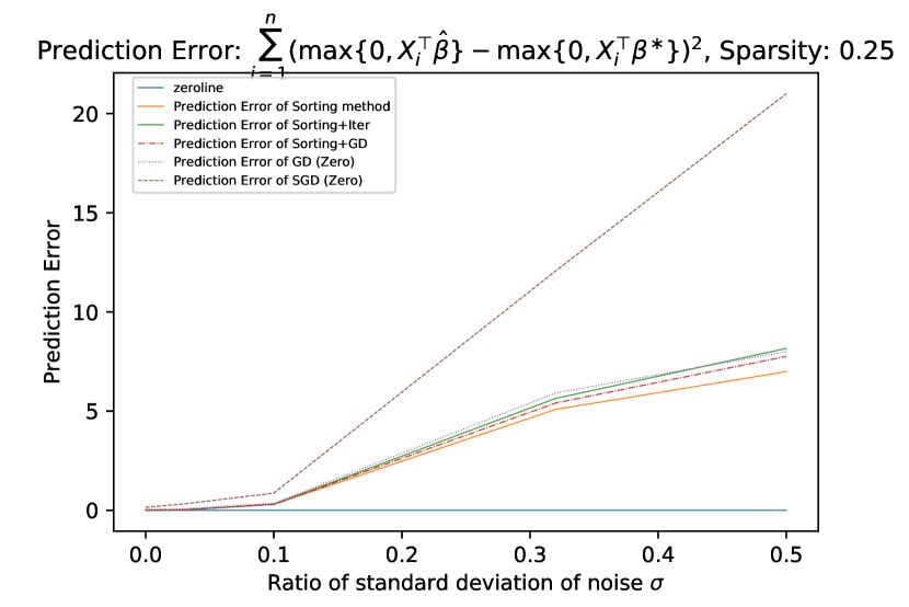
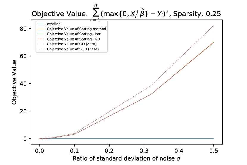
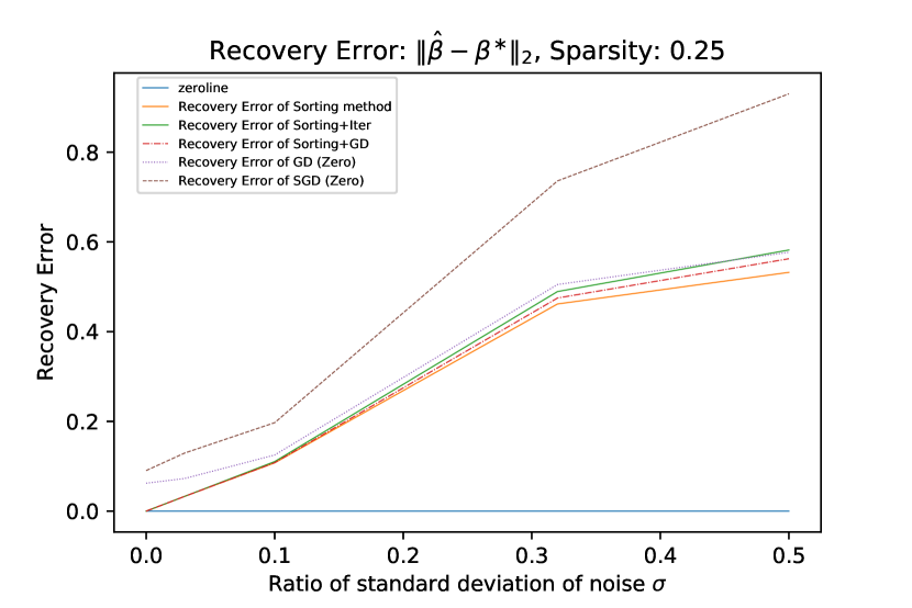
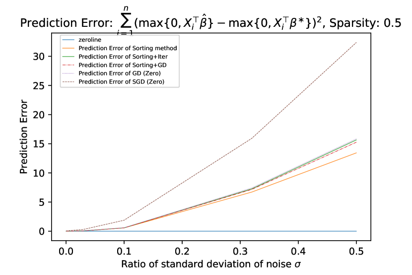
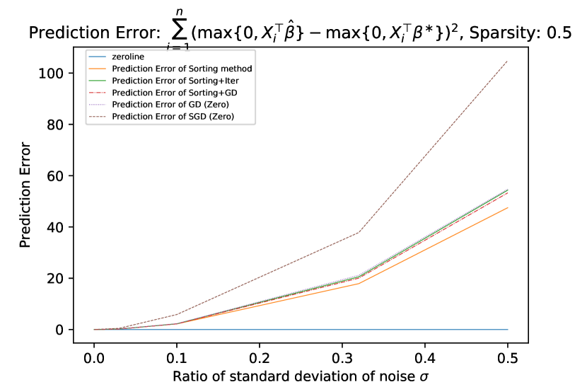
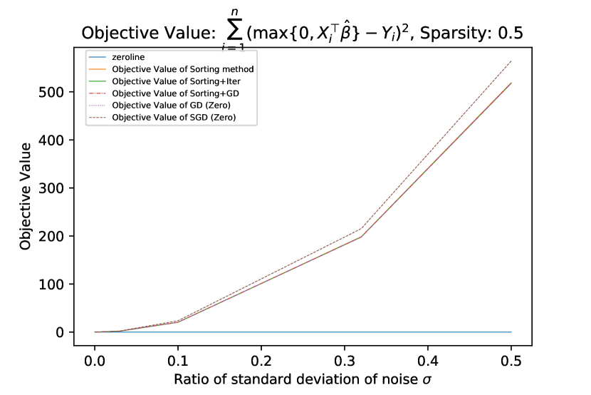
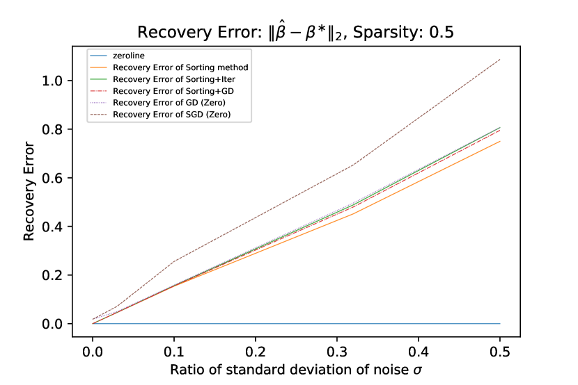
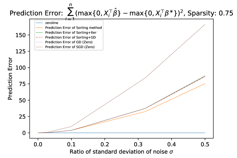
In this section, we empirically compare the numerical results of four methods: sorting method (a simplified version of AlgorithmΒ 1, we describe this below in this section), sorting followed by an iterative heuristics (we describe this heuristic below in this section), gradient descent method starting at origin, sorting followed by gradient descent method, stochastic gradient method on synthetic instances for the One-Node-ReLU problem. A feasible solution Ξ²^^𝛽\hat{\beta} that obtained from above methods is evaluated in terms of its prediction error, objective value, recovery error and generalization error. In the rest of this section, details and settings are presented.

3.1 Hardware & Software

All numerical experiments are implemented on MacBookPro13 with 2 GHz Intel Core i5 CPU and 8 GB 1867 MHz LPDDR3 Memory. Each optimization step of sorting method (AlgorithmΒ 1) and each optimization step of iterative method (AlgorithmΒ 3) are solved using Gurobi 7.0.2. in python 3.5.3.

3.2 Synthetic Instances

We perform numerical experiments on the following type of instances.

  1. 1.

    Given a vector ΞΌβˆˆβ„pπœ‡superscriptℝ𝑝\mu\in\mathbb{R}^{p}, and a positive semidefinite matrix Ξ£βˆˆβ„pΓ—pΞ£superscriptℝ𝑝𝑝\Sigma\in\mathbb{R}^{p\times p}, the true solution Ξ²βˆ—superscriptπ›½βˆ—\beta^{\ast} is generated from the Gaussian distribution N​(ΞΌ,Ξ£)π‘πœ‡Ξ£N(\mu,\Sigma). Specifically, Ξ²βˆ—superscriptπ›½βˆ—\beta^{\ast} in FigureΒ [5, 6, 3] are generated from N​(0.5β‹…πŸŽp,10β‹…Ip)𝑁⋅0.5subscript0𝑝⋅10subscript𝐼𝑝N(0.5\cdot\mathbf{0}_{p},10\cdot I_{p}).

  2. 2.

    Both training set and testing set contain n𝑛n sample points. For each sample point (Xi,Yi)βˆˆβ„p×ℝsubscript𝑋𝑖subscriptπ‘Œπ‘–superscriptℝ𝑝ℝ(X_{i},Y_{i})\in\mathbb{R}^{p}\times\mathbb{R} in training set, the observation sample Xi=(Xi​j)j=1psubscript𝑋𝑖superscriptsubscriptsubscript𝑋𝑖𝑗𝑗1𝑝X_{i}=(X_{ij})_{j=1}^{p} is generated by setting each component Xi​j=1,Xi​j=βˆ’1formulae-sequencesubscript𝑋𝑖𝑗1subscript𝑋𝑖𝑗1X_{ij}=1,X_{ij}=-1 with probability P2𝑃2\frac{P}{2} and Xi​j=0subscript𝑋𝑖𝑗0X_{ij}=0 with probability 1βˆ’P1𝑃1-P independently. In the rest of this sections, we denote the probability P=ℙ​({Xi​j=1}βˆͺ{Xi​j=βˆ’1})𝑃ℙsubscript𝑋𝑖𝑗1subscript𝑋𝑖𝑗1P=\mathbb{P}(\{X_{ij}=1\}\cup\{X_{ij}=-1\}) as the level of sparsity, i.e., the higher the level of sparsity, the more number of non-zero components exists in Xisubscript𝑋𝑖X_{i} in expectation.

    Moreover, in the realizable case we perturbed the data to guarantee that the global optimal solution is unique. Assuming that Ξ²iβˆ—β‰ 0subscriptsuperscript𝛽𝑖0\beta^{*}_{i}\neq 0 for all i∈[p]𝑖delimited-[]𝑝i\in[p], the first p𝑝p samples Xisubscript𝑋𝑖X_{i} are obtained as Xi←eiβ‹…sgn​(Ξ²iβˆ—)←subscript𝑋𝑖⋅subscript𝑒𝑖sgnsuperscriptsubscriptπ›½π‘–βˆ—X_{i}\leftarrow e_{i}\cdot\text{sgn}(\beta_{i}^{\ast}) for all i=1,…,p𝑖1…𝑝i=1,\ldots,p in training set, in which eiβˆˆβ„psubscript𝑒𝑖superscriptℝ𝑝e_{i}\in\mathbb{R}^{p} is a vector with 1 on its ithsuperscript𝑖thi^{\text{th}} component and 0 on rest, and sgn​(x)={1Β if ​x>0βˆ’1Β otherwisesgnπ‘₯cases1Β ifΒ π‘₯0missing-subexpression1Β otherwisemissing-subexpression\text{sgn}(x)=\left\{\begin{array}[]{lll}1&\text{ if }x>0\\ -1&\text{ otherwise}\end{array}\right..

  3. 3.

    Note the constant term Ξ²0βˆ—superscriptsubscript𝛽0βˆ—\beta_{0}^{\ast} can be achieved via adding one additional dimension with component 1 to each Xisubscript𝑋𝑖X_{i}. To simplify, we deiced to use Ξ²0βˆ—=0subscriptsuperscript𝛽00\beta^{*}_{0}=0. The response sample Yisubscriptπ‘Œπ‘–Y_{i} is therefore computed as Yi=max⁑{0,XiβŠ€β€‹Ξ²βˆ—}+Ο΅isubscriptπ‘Œπ‘–0superscriptsubscript𝑋𝑖topsuperscriptπ›½βˆ—subscriptitalic-ϡ𝑖Y_{i}=\max\{0,X_{i}^{\top}\beta^{\ast}\}+\epsilon_{i} with Ο΅i∼N​(0,ρ​σ)similar-tosubscriptitalic-ϡ𝑖𝑁0𝜌𝜎\epsilon_{i}\sim N(0,\rho\sigma) where ΟƒπœŽ\sigma and ρ𝜌\rho are set in the following way:

    ΟƒπœŽ\sigma:

    (1) Let Zi←XiβŠ€β€‹Ξ²βˆ—β†subscript𝑍𝑖superscriptsubscript𝑋𝑖topsuperscriptπ›½βˆ—Z_{i}\leftarrow X_{i}^{\top}\beta^{\ast} for all i=1,…,n𝑖1…𝑛i=1,\ldots,n. (2) Compute the average of {Zi}i=1nsuperscriptsubscriptsubscript𝑍𝑖𝑖1𝑛\{Z_{i}\}_{i=1}^{n} as Z¯←1nβ€‹βˆ‘i=1nZi←¯𝑍1𝑛superscriptsubscript𝑖1𝑛subscript𝑍𝑖\bar{Z}\leftarrow\frac{1}{n}\sum_{i=1}^{n}Z_{i}. (3) Set Οƒ2←1nβ€‹βˆ‘i=1n(Ziβˆ’ZΒ―)2←superscript𝜎21𝑛superscriptsubscript𝑖1𝑛superscriptsubscript𝑍𝑖¯𝑍2\sigma^{2}\leftarrow\frac{1}{n}\sum_{i=1}^{n}(Z_{i}-\bar{Z})^{2}.

    ρ𝜌\rho:

    Since the noise levels are commonly measured in signal-to-noise decibels (dB), we examined dB values {6,10,20,30,∞}6102030\{6,10,20,30,\infty\}, then the value of signal-to-noise ratio ρ𝜌\rho can be computed from

    dBβ‰œ10​log10⁑(Οƒ2ρ2​σ2)∈{6,10,20,30,∞}β‰œdB10subscript10superscript𝜎2superscript𝜌2superscript𝜎26102030\displaystyle\text{dB}\triangleq 10\log_{10}\left(\frac{\sigma^{2}}{\rho^{2}\sigma^{2}}\right)\in\{6,10,20,30,\infty\}

    which corresponds to Οβ‰ˆ{0.5,0.32,0.1,0.032,0}𝜌0.50.320.10.0320\rho\approx\{0.5,0.32,0.1,0.032,0\}.

  4. 4.

    For each sample point (X~i,Y~i)βˆˆβ„p×ℝsubscript~𝑋𝑖subscript~π‘Œπ‘–superscriptℝ𝑝ℝ(\tilde{X}_{i},\tilde{Y}_{i})\in\mathbb{R}^{p}\times\mathbb{R} in testing set, generate X~i,Y~isubscript~𝑋𝑖subscript~π‘Œπ‘–\tilde{X}_{i},\tilde{Y}_{i} in the same way as the training set.

3.3 Algorithms

In this section, we briefly describe the algorithms that were tested in the numerical experiments.

3.3.1 Method 1: Sorting Method (sorting)

The sorting method is a simplied and slightly cruder version of AlgorithmΒ 1 with parameter k=1π‘˜1k=1. Essentially, in order to reduce the running time, instead of i1subscript𝑖1i_{1} taking all values from 111 to n𝑛n, we limit the values of i1subscript𝑖1i_{1} that are used, see details in SectionΒ A.

3.3.2 Method 2: Sorting method followed by an Iterative Method (sorting + iterative)

A natural iterative improving algorithm is the following: Fix I𝐼I and minimize fσ​(I)superscriptπ‘“πœŽπΌf^{\sigma}(I). Now, examine the solution and update the choice of I𝐼I which so the fΟƒsuperscriptπ‘“πœŽf^{\sigma} and fβˆ—superscript𝑓f^{*} match for the current solution. Repeat until some stopping criteria is meet. See in Algorithm 3 in SectionΒ B for details.

We use this heuristic to improve the solution obtained from the sorting method. After obtaining a feasible solution Ξ²^sortingsuperscript^𝛽sorting\hat{\beta}^{\text{sorting}}, we set the initial point of iterative heurisitic as Ξ²^sortingsuperscript^𝛽sorting\hat{\beta}^{\text{sorting}}.

3.3.3 Method 3: Gradient Descent Method (GD)

The gradient descent method used in numerical experiments is presented in SectionΒ C, see AlgorithmΒ 4. Given the initial point Ξ²0β†πŸŽp←superscript𝛽0subscript0𝑝\beta^{0}\leftarrow\mathbf{0}_{p}, and set Ξ²tsuperscript𝛽𝑑\beta^{t} as the updated solution obtained in (tβˆ’1)thsuperscript𝑑1th(t-1)^{\text{th}} iteration, the gradient used in tthsuperscript𝑑tht^{\text{th}} iteration is:

1nβ€‹βˆ‡Ξ²L​(Ξ²t)=1nβ€‹βˆ‘i=1n(max⁑{0,XiβŠ€β€‹Ξ²t}βˆ’Yi)​(1+sgn​(XiβŠ€β€‹Ξ²t))​Xi1𝑛subscriptβˆ‡π›½πΏsuperscript𝛽𝑑1𝑛superscriptsubscript𝑖1𝑛0superscriptsubscript𝑋𝑖topsuperscript𝛽𝑑subscriptπ‘Œπ‘–1sgnsuperscriptsubscript𝑋𝑖topsuperscript𝛽𝑑subscript𝑋𝑖\displaystyle\frac{1}{n}\nabla_{\beta}L(\beta^{t})=\frac{1}{n}\sum_{i=1}^{n}(\max\{0,X_{i}^{\top}\beta^{t}\}-Y_{i})(1+\text{sgn}(X_{i}^{\top}\beta^{t}))X_{i}

where L​(Ξ²)β†βˆ‘i=1n(max⁑{0,XiβŠ€β€‹Ξ²}βˆ’Yi)2←𝐿𝛽superscriptsubscript𝑖1𝑛superscript0superscriptsubscript𝑋𝑖top𝛽subscriptπ‘Œπ‘–2L(\beta)\leftarrow\sum_{i=1}^{n}(\max\{0,X_{i}^{\top}\beta\}-Y_{i})^{2} and sgn​(x)={1Β if ​x>0βˆ’1Β if ​x≀0sgnπ‘₯cases1Β ifΒ π‘₯0missing-subexpression1Β ifΒ π‘₯0missing-subexpression\text{sgn}(x)=\left\{\begin{array}[]{lll}1&\text{ if }x>0\\ -1&\text{ if }x\leq 0\end{array}\right..

3.3.4 Method 4: Sorting followed by Gradient Descent Method (sorting + GD)

Similar to the sorting followed by gradient descent method, in this method we run the sorting method and then use the final solution of the sorting method as the starting point for gradient descent.

3.3.5 Method 5: Stochastic Gradient Descent Method (SGD)

The initial point Ξ²0superscript𝛽0\beta^{0} used in stochastic gradient descent (SGD) method is the same as gradient descent (GD) method, i.e. the origin. The only difference between SGD and GD is that: in tthsuperscript𝑑tht^{\text{th}} iteration, we uniformly pick a mini-batch Btsuperscript𝐡𝑑B^{t} of size mπ‘šm from the set of samples {(Xi,Yi)}i=1nsuperscriptsubscriptsubscript𝑋𝑖subscriptπ‘Œπ‘–π‘–1𝑛\{(X_{i},Y_{i})\}_{i=1}^{n} at random, then the gradient used in tthsuperscript𝑑tht^{\text{th}} iteration is:

1mβ€‹βˆ‘i∈St(max⁑{0,XiβŠ€β€‹Ξ²t}βˆ’Yi)​(1+sgn​(XiβŠ€β€‹Ξ²t))​Xi,1π‘šsubscript𝑖superscript𝑆𝑑0superscriptsubscript𝑋𝑖topsuperscript𝛽𝑑subscriptπ‘Œπ‘–1sgnsuperscriptsubscript𝑋𝑖topsuperscript𝛽𝑑subscript𝑋𝑖\displaystyle\frac{1}{m}\sum_{i\in S^{t}}(\max\{0,X_{i}^{\top}\beta^{t}\}-Y_{i})(1+\text{sgn}(X_{i}^{\top}\beta^{t}))X_{i},

with sgn​(x)={1Β if ​x>0βˆ’1Β if ​x≀0sgnπ‘₯cases1Β ifΒ π‘₯0missing-subexpression1Β ifΒ π‘₯0missing-subexpression\text{sgn}(x)=\left\{\begin{array}[]{lll}1&\text{ if }x>0\\ -1&\text{ if }x\leq 0\end{array}\right.. See AlgorithmΒ 5.

3.4 Measures

The feasible solutions Ξ²^^𝛽\hat{\beta} obtained from the above five methods are evaluated in terms of their prediction error, objective value, recovery error, generalization error. The formal definitions of these three types of errors are:

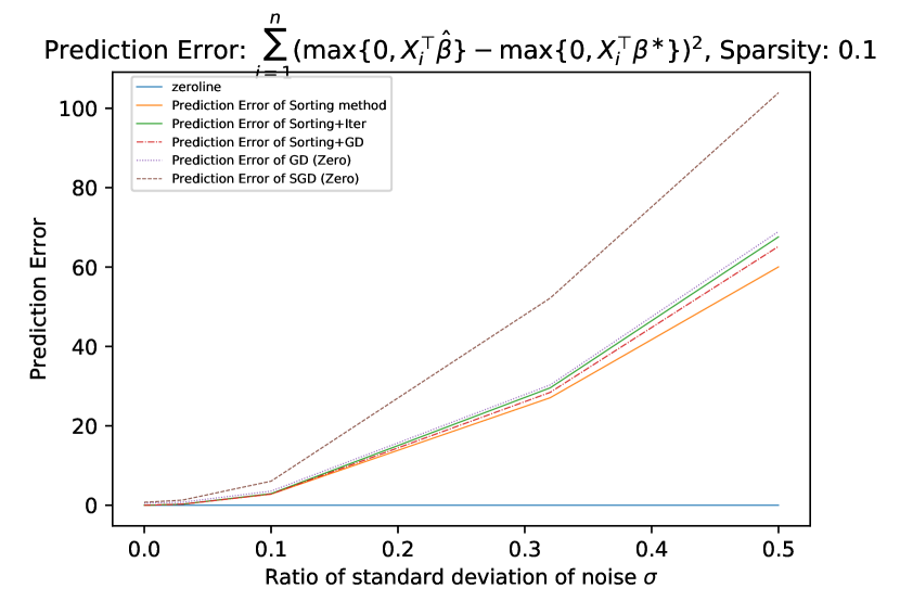
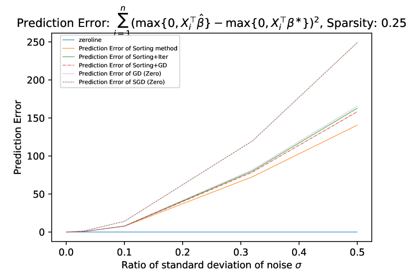
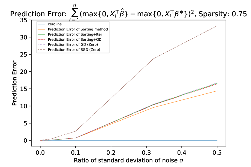
Prediction Error:

The prediction error is defined based on the provided solution Ξ²^^𝛽\hat{\beta}, i.e.,

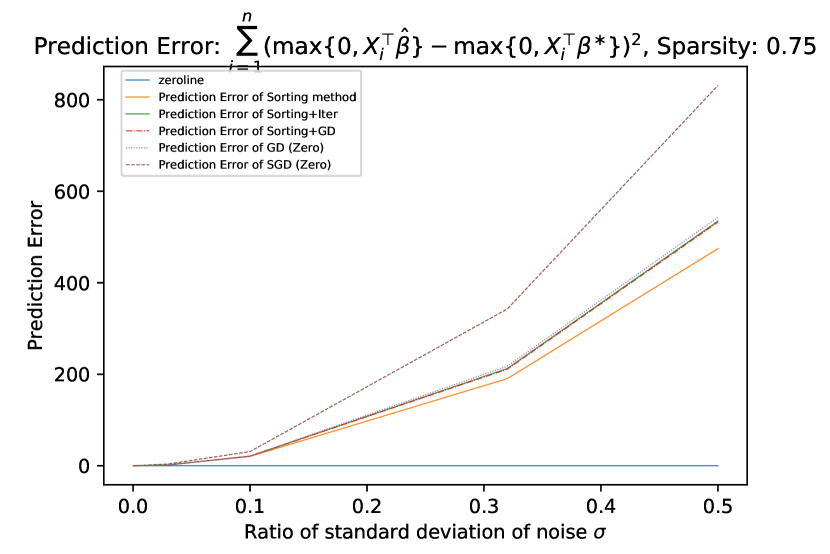
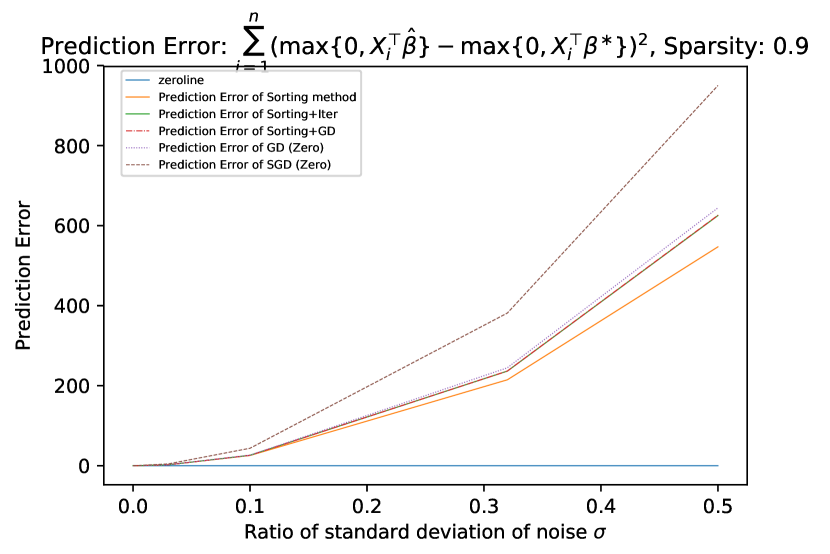
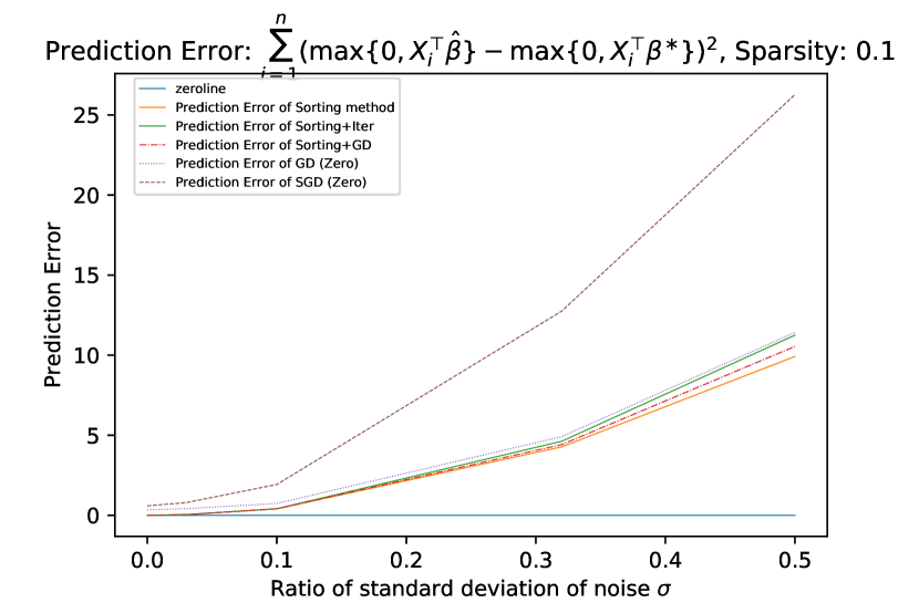
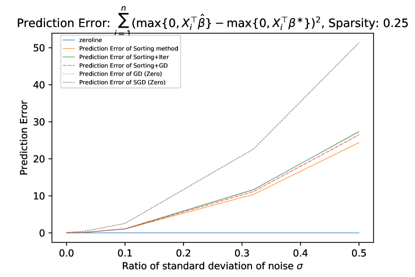
PEβ‰œβˆ‘i=1n(max⁑{0,XiβŠ€β€‹Ξ²^}βˆ’max⁑{0,XiβŠ€β€‹Ξ²βˆ—})2,where​{Xi,Yi}i=1n​ is training data.β‰œPEsuperscriptsubscript𝑖1𝑛superscript0superscriptsubscript𝑋𝑖top^𝛽0superscriptsubscript𝑋𝑖topsuperscriptπ›½βˆ—2wheresuperscriptsubscriptsubscript𝑋𝑖subscriptπ‘Œπ‘–π‘–1𝑛 is training data\text{PE}\triangleq\sum_{i=1}^{n}\left(\max\{0,X_{i}^{\top}\hat{\beta}\}-\max\{0,X_{i}^{\top}\beta^{\ast}\}\right)^{2},\quad\textup{where}\{X_{i},Y_{i}\}_{i=1}^{n}\textup{ is training data}.
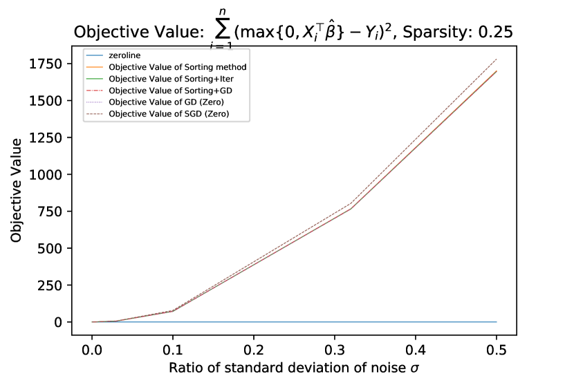
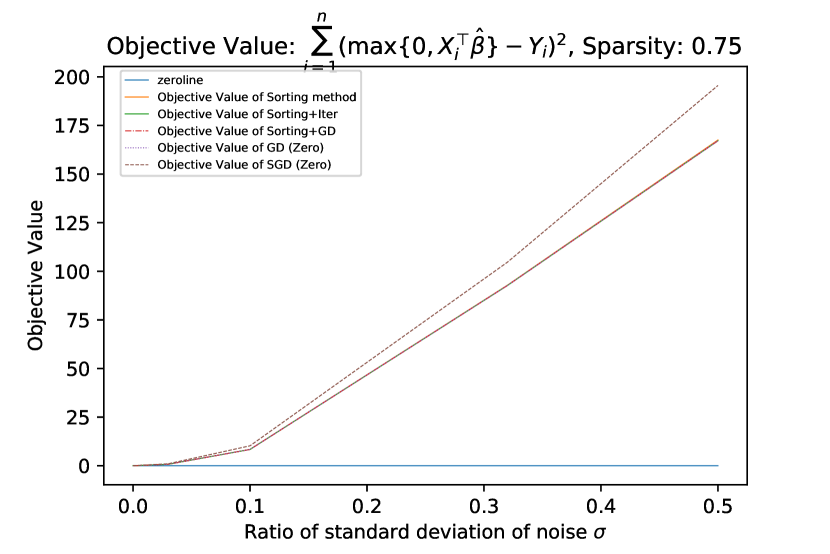
Objective Value:

Note that the prediction error defined as above is not the objective value obtained from above five methods. Actually, in practice, when Ξ²βˆ—superscriptπ›½βˆ—\beta^{\ast} is unknown, the prediction error cannot be obtained exactly, thus one may use objective value (Obj)

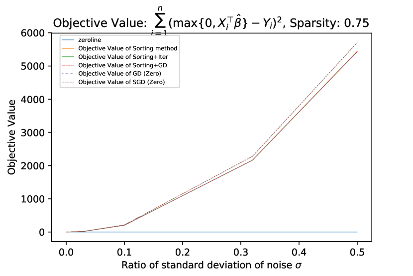
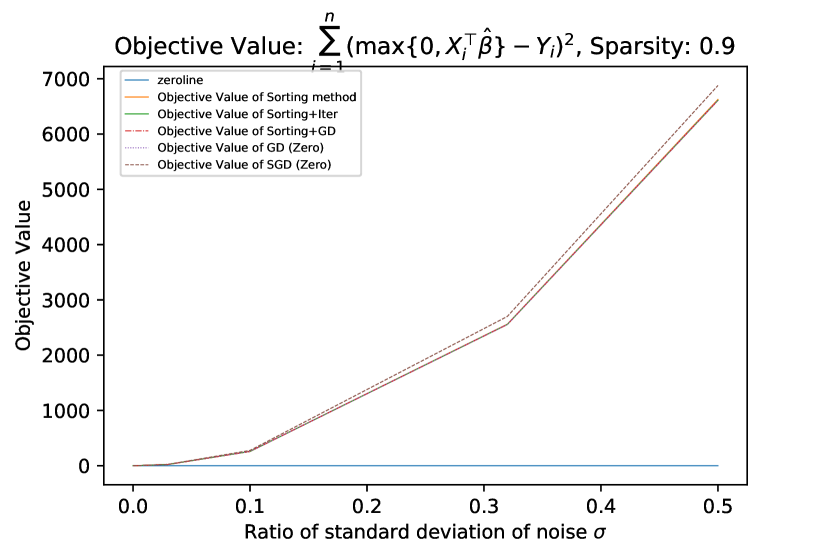
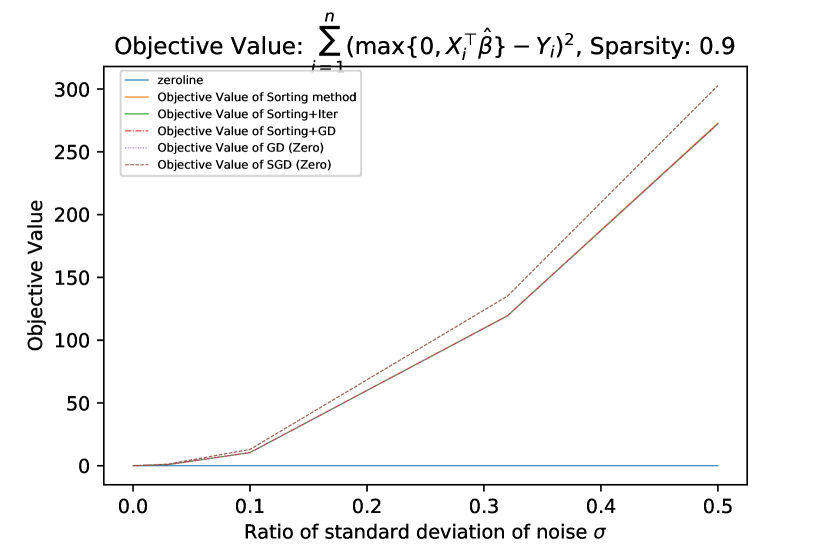
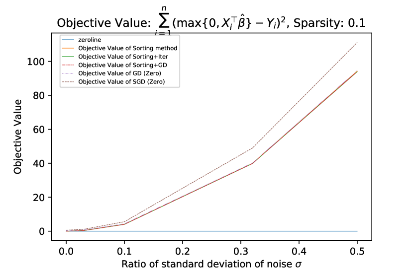
Objβ‰œβˆ‘i=1n(max⁑{0,XiβŠ€β€‹Ξ²^}βˆ’Yi)2,where​{Xi,Yi}i=1n​ is training data.β‰œObjsuperscriptsubscript𝑖1𝑛superscript0superscriptsubscript𝑋𝑖top^𝛽subscriptπ‘Œπ‘–2wheresuperscriptsubscriptsubscript𝑋𝑖subscriptπ‘Œπ‘–π‘–1𝑛 is training data\displaystyle\text{Obj}\triangleq\sum_{i=1}^{n}\left(\max\{0,X_{i}^{\top}\hat{\beta}\}-Y_{i}\right)^{2},\quad\textup{where}\{X_{i},Y_{i}\}_{i=1}^{n}\textup{ is training data}.

as an alternative.

Recovery Error:

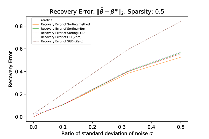
The recovery error measures the distance between the solution Ξ²^^𝛽\hat{\beta} we obtained and the ground truth Ξ²βˆ—superscriptπ›½βˆ—\beta^{\ast}, which is

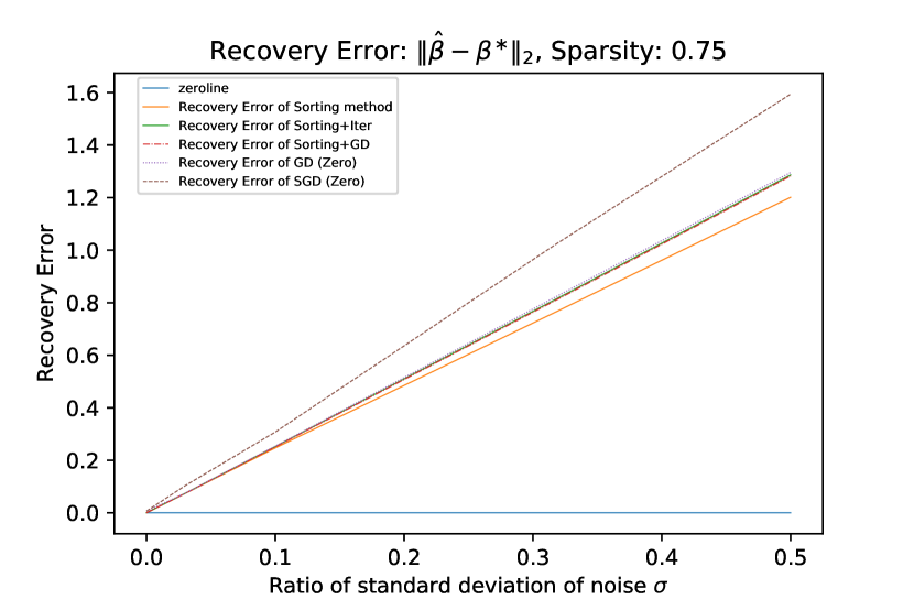
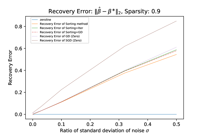
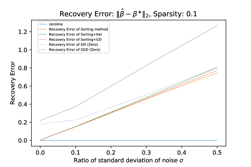
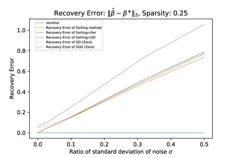
REβ‰œβ€–Ξ²^βˆ’Ξ²βˆ—β€–2.β‰œREsubscriptnorm^𝛽superscriptπ›½βˆ—2\text{RE}\triangleq\|\hat{\beta}-\beta^{\ast}\|_{2}.
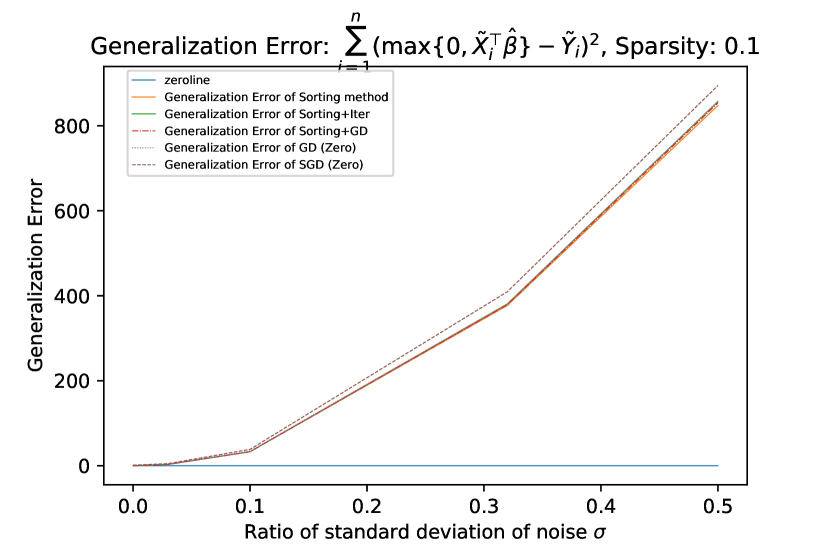
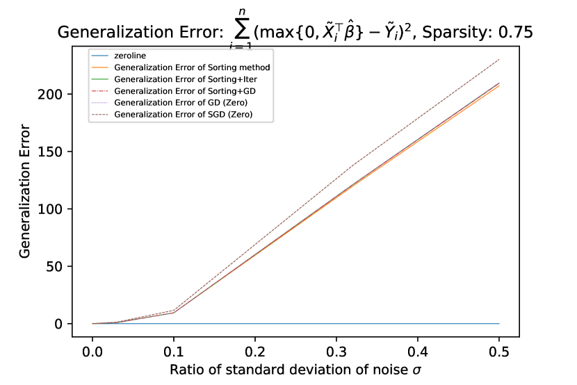
Generalization Error:

The generalization error measures how good the solution Ξ²^^𝛽\hat{\beta} is, when using the objective function with resect to testing set, i.e.

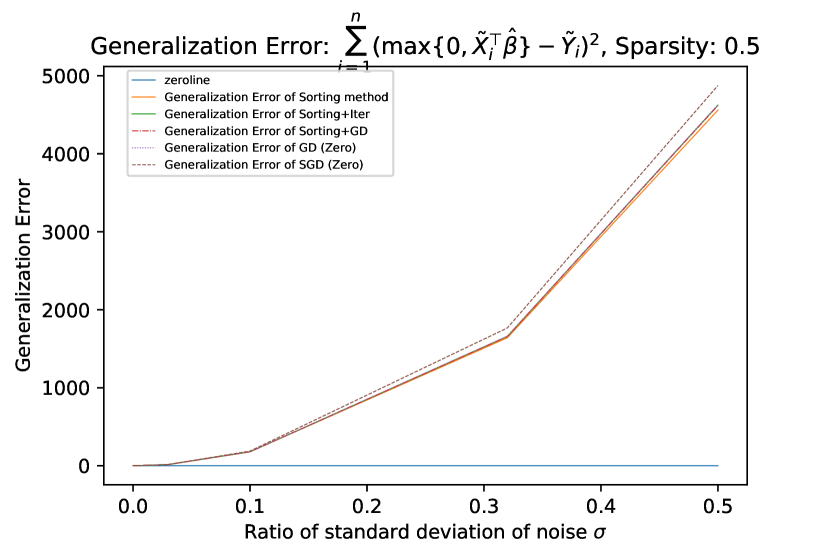
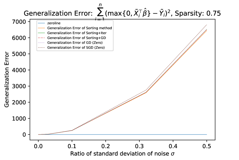
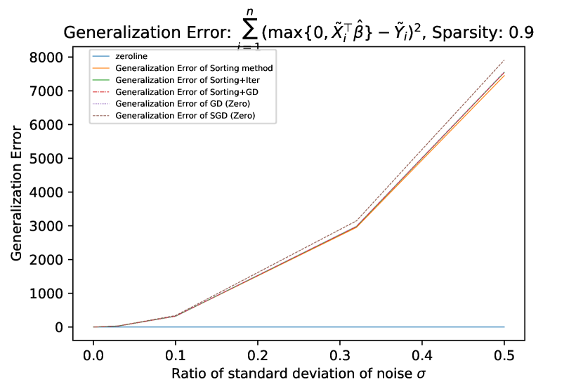
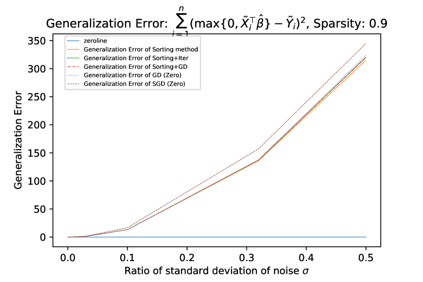
GEβ‰œβˆ‘i=1n(max⁑{0,X~iβŠ€β€‹Ξ²^}βˆ’Y~i)2,where​{Xi,Yi}i=1n​ is testing data.β‰œGEsuperscriptsubscript𝑖1𝑛superscript0superscriptsubscript~𝑋𝑖top^𝛽subscript~π‘Œπ‘–2wheresuperscriptsubscriptsubscript𝑋𝑖subscriptπ‘Œπ‘–π‘–1𝑛 is testing data\text{GE}\triangleq\sum_{i=1}^{n}\left(\max\{0,\tilde{X}_{i}^{\top}\hat{\beta}\}-\tilde{Y}_{i}\right)^{2},\quad\textup{where}\{X_{i},Y_{i}\}_{i=1}^{n}\textup{ is testing data}.

We note that in order to see the comparison between different methods more clearly, the prediction error and generalization error are not divided by the size of sample set n𝑛n.

3.5 Numerical Results: Notation and Parameters

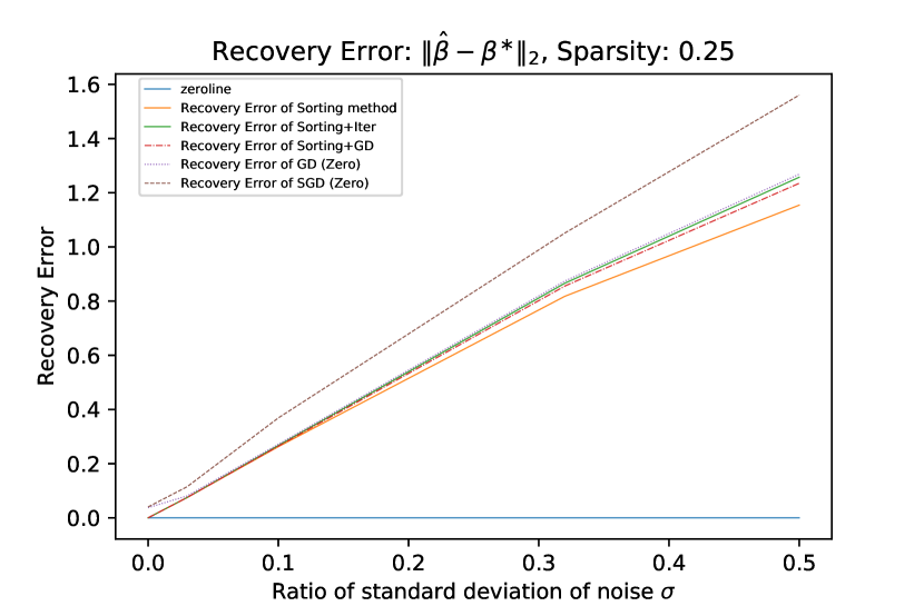
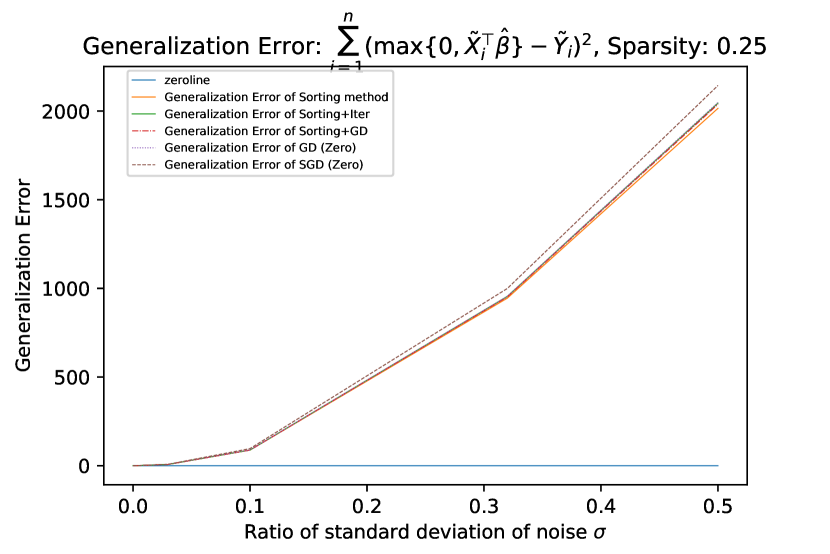
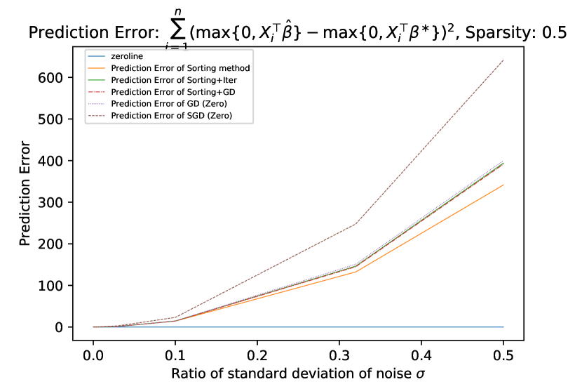
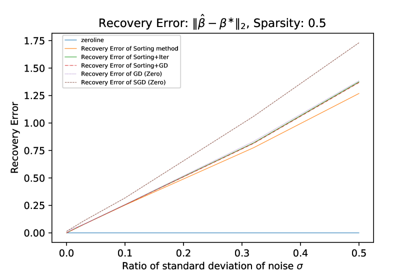
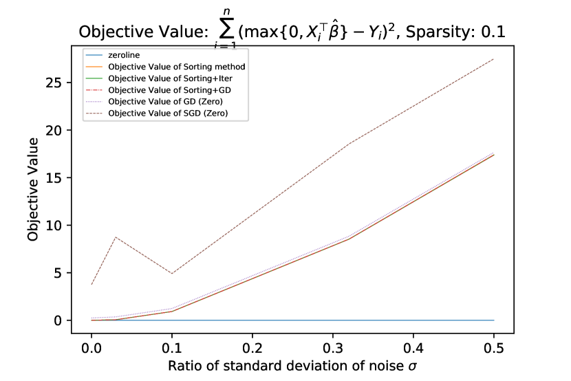
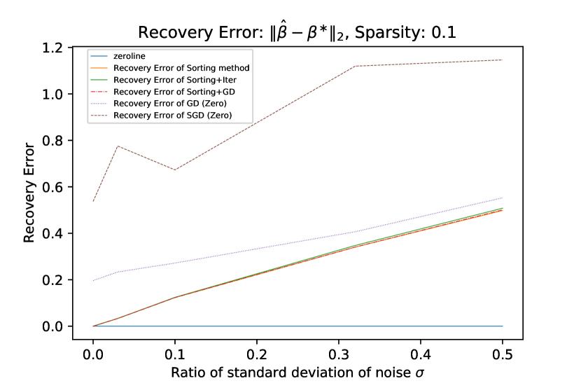
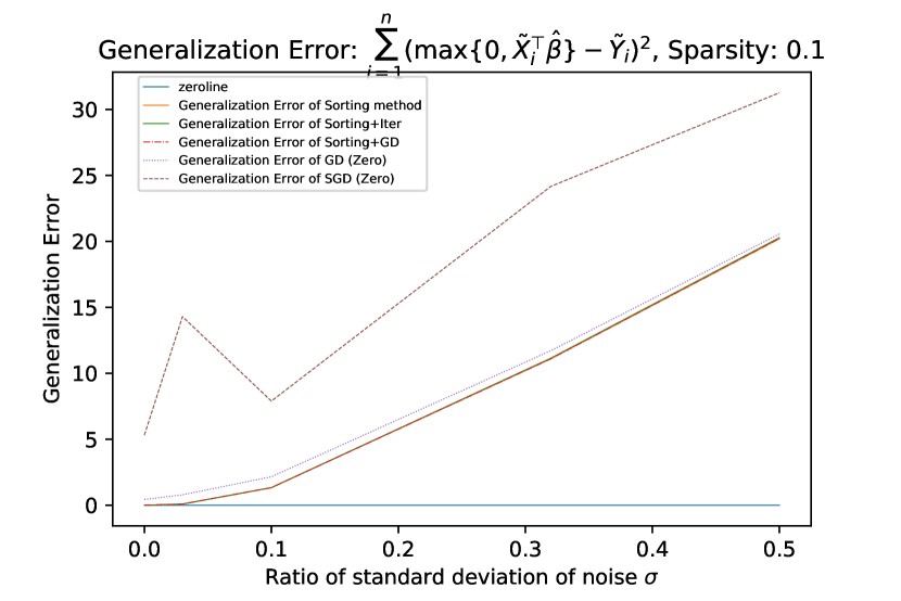
The numerical results in FigureΒ [3] of this section, and in FigureΒ [5, 6] in AppendixΒ E present how these measures (prediction error, recovery error, generalization error) and the running time change depending on different standard deviation of noise empirically. The detailed realizable cases in AppendixΒ F provide an empirical result of the performances of previous four methods. Below we present notations and the parameters that used for numerical experiments:

  • β€’

    Each line presented in FigureΒ [5, 6, 3] represents the average of the measures or running time obtained from 20 instances under the same settings.

  • β€’

    The first column of each Table in AppendixΒ F is a tuple of 4 elements (p,n,ρ;index)π‘π‘›πœŒindex(p,n,\rho;\text{index}) which represents the dimension of β𝛽\beta, the number of training samples, the ratio used for noise Ο΅isubscriptitalic-ϡ𝑖\epsilon_{i}, and the index of the instance with such settings respectively.

  • β€’

    For the Sorting Method (AlgorithmΒ 2), N𝑁N (the number of splits) used is 101010.

  • β€’

    For the Sorting (AlgorithmΒ 2) + Iterative Method (AlgorithmΒ 3), N𝑁N (the number of split) is set to 101010, and let Ξ²^sortingsuperscript^𝛽sorting\hat{\beta}^{\text{sorting}} be the solution obtained from Sorting Method, then the parameters of Iterative Method are set to be:

    ({(Xi,Yi)}i=1n,Ξ²0,T)←({(Xi,Yi)}i=1n,Ξ²^sorting,20)←superscriptsubscriptsubscript𝑋𝑖subscriptπ‘Œπ‘–π‘–1𝑛superscript𝛽0𝑇superscriptsubscriptsubscript𝑋𝑖subscriptπ‘Œπ‘–π‘–1𝑛superscript^𝛽sorting20\displaystyle(\{(X_{i},Y_{i})\}_{i=1}^{n},\beta^{0},T)\leftarrow(\{(X_{i},Y_{i})\}_{i=1}^{n},\hat{\beta}^{\text{sorting}},20)

    where Ξ²0superscript𝛽0\beta^{0} denotes the starting point, T𝑇T denotes the maximum number of iterations.

  • β€’

    For the Gradient Descent Method (AlgorithmΒ 4), the parameters are set to be

    ({(Xi,Yi)}i=1n,Ξ²0,T,Ο΅,Ξ·0,Ξ³,Ξ±)←({(Xi,Yi)}i=1n,𝟎p,1000,0.01,1,0.03,0.6)←superscriptsubscriptsubscript𝑋𝑖subscriptπ‘Œπ‘–π‘–1𝑛superscript𝛽0𝑇italic-Ο΅subscriptπœ‚0𝛾𝛼superscriptsubscriptsubscript𝑋𝑖subscriptπ‘Œπ‘–π‘–1𝑛subscript0𝑝10000.0110.030.6\displaystyle(\{(X_{i},Y_{i})\}_{i=1}^{n},\beta^{0},T,\epsilon,\eta_{0},\gamma,\alpha)\leftarrow(\{(X_{i},Y_{i})\}_{i=1}^{n},\mathbf{0}_{p},1000,0.01,1,0.03,0.6)

    where Ξ²0superscript𝛽0\beta^{0} denotes the starting point, T𝑇T denotes the maximum number of iterations, Ο΅italic-Ο΅\epsilon is a termination criteria parameter, Ξ·0subscriptπœ‚0\eta_{0} denotes the initial stepsize, Ξ³,α𝛾𝛼\gamma,\alpha are parameters used to adjust stepsize in each iteration.

  • β€’

    For the Sorting (AlgorithmΒ 2) + Gradient Descent Method (AlgorithmΒ 4), N𝑁N (the number of split) is set to be 101010, and let Ξ²^sortingsuperscript^𝛽sorting\hat{\beta}^{\text{sorting}} is as above, and the parameters of the Gradient Descent Method are set to be:

    ({(Xi,Yi)}i=1n,Ξ²0,T,Ο΅,Ξ·0,Ξ³,Ξ±)←({(Xi,Yi)}i=1n,Ξ²^sorting,1000,0.01,1,0.03,0.6).←superscriptsubscriptsubscript𝑋𝑖subscriptπ‘Œπ‘–π‘–1𝑛superscript𝛽0𝑇italic-Ο΅subscriptπœ‚0𝛾𝛼superscriptsubscriptsubscript𝑋𝑖subscriptπ‘Œπ‘–π‘–1𝑛superscript^𝛽sorting10000.0110.030.6\displaystyle(\{(X_{i},Y_{i})\}_{i=1}^{n},\beta^{0},T,\epsilon,\eta_{0},\gamma,\alpha)\leftarrow(\{(X_{i},Y_{i})\}_{i=1}^{n},\hat{\beta}^{\text{sorting}},1000,0.01,1,0.03,0.6).
  • β€’

    For the Stochastic Gradient Descent Method (AlgorithmΒ 5), parameters are set to be:
    ({(Xi,Yi)}i=1n,Ξ²0,T,Ο΅,Ξ·0,Ξ³,Ξ±,m)←({(Xi,Yi)}i=1n,𝟎p,1000,0.01,1,0.03,0.6,⌊0.1​nβŒ‹).←superscriptsubscriptsubscript𝑋𝑖subscriptπ‘Œπ‘–π‘–1𝑛superscript𝛽0𝑇italic-Ο΅subscriptπœ‚0π›Ύπ›Όπ‘šsuperscriptsubscriptsubscript𝑋𝑖subscriptπ‘Œπ‘–π‘–1𝑛subscript0𝑝10000.0110.030.60.1𝑛\displaystyle(\{(X_{i},Y_{i})\}_{i=1}^{n},\beta^{0},T,\epsilon,\eta_{0},\gamma,\alpha,m)\leftarrow(\{(X_{i},Y_{i})\}_{i=1}^{n},\mathbf{0}_{p},1000,0.01,1,0.03,0.6,\lfloor 0.1n\rfloor).
Refer to caption
(a) Prediction Error
Refer to caption
(b) Objective Value
Refer to caption
(c) Recovery Error
Refer to caption
(d) Generalization Error
Refer to caption
(e) Prediction Error
Refer to caption
(f) Objective Value
Refer to caption
(g) Recovery Error
Refer to caption
(h) Generalization Error
Refer to caption
(i) Prediction Error
Refer to caption
(j) Objective Value
Refer to caption
(k) Recovery Error
Refer to caption
(l) Generalization Error
Refer to caption
(m) Prediction Error
Refer to caption
(n) Objective Value
Refer to caption
(o) Recovery Error
Refer to caption
(p) Generalization Error
Refer to caption
(q) Prediction Error
Refer to caption
(r) Objective Value
Refer to caption
(s) Recovery Error
Refer to caption
(t) Generalization Error
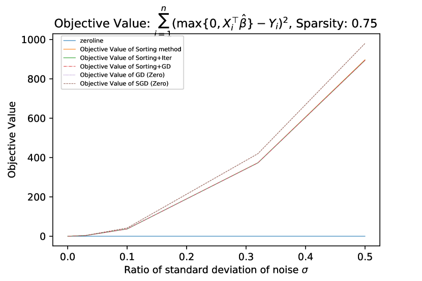
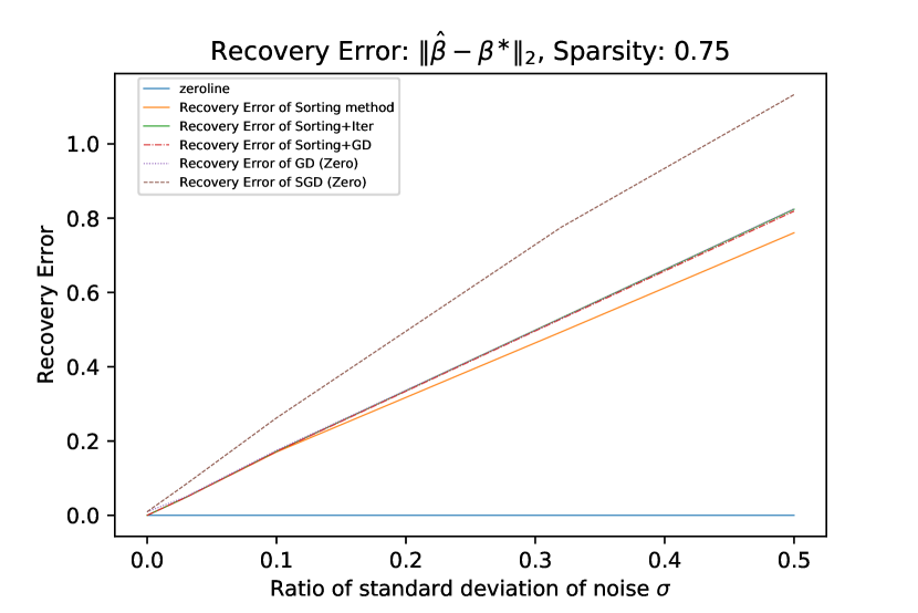
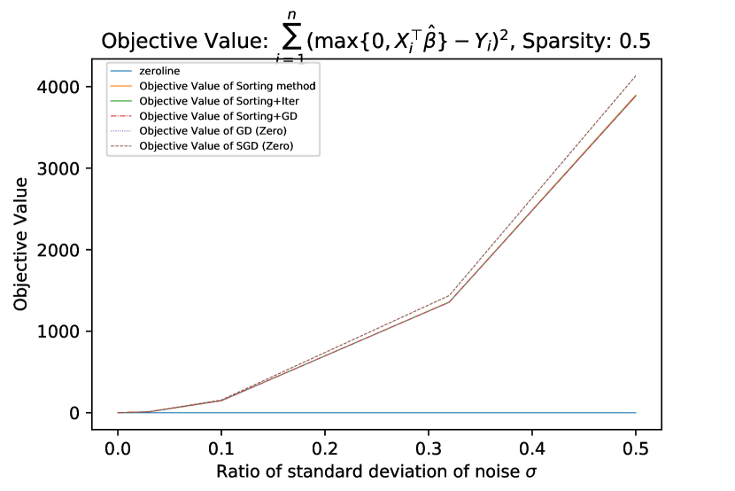
Figure 3: Numerical Results of sample size (p,n)=(50,1000)𝑝𝑛501000(p,n)=(50,1000) and Ξ²βˆ—βˆΌN​(0.5β‹…πŸp,50β‹…Ip)similar-tosuperscriptπ›½βˆ—π‘β‹…0.5subscript1𝑝⋅50subscript𝐼𝑝\beta^{\ast}\sim N(0.5\cdot\mathbf{1}_{p},50\cdot I_{p}) with sparsity {0.1,0.25,0.5,0.75,0.9}0.10.250.50.750.9\{0.1,0.25,0.5,0.75,0.9\}

3.6 Summary of Numerical Experiments

Based on the results reported in FigureΒ [5, 6, 3] and Tables in AppendixΒ F, some preliminary conclusions can be draw as follows:

Prediction Error:

The empirical prediction error satisfies the following:

PEsorting≀PEsorting + iter≀PEsorting + GD≀PEGD≀PESGDsuperscriptPEsortingsuperscriptPEsorting + itersuperscriptPEsorting + GDsuperscriptPEGDsuperscriptPESGD\displaystyle\text{PE}^{\text{sorting}}\leq\text{PE}^{\text{sorting + iter}}\leq\text{PE}^{\text{sorting + GD}}\leq\text{PE}^{\text{GD}}\leq\text{PE}^{\text{SGD}}

where the differences between PEsorting + iter,PEsorting + GD,PEGDsuperscriptPEsorting + itersuperscriptPEsorting + GDsuperscriptPEGD\text{PE}^{\text{sorting + iter}},\text{PE}^{\text{sorting + GD}},\text{PE}^{\text{GD}} are relative small than the differences between PEsorting,PEsorting + itersuperscriptPEsortingsuperscriptPEsorting + iter\text{PE}^{\text{sorting}},\text{PE}^{\text{sorting + iter}} and PEGD,PESGDsuperscriptPEGDsuperscriptPESGD\text{PE}^{\text{GD}},\text{PE}^{\text{SGD}}. These empirical results show that the when the output samples {Yi}subscriptπ‘Œπ‘–\{Y_{i}\} follows the correct underlying model (which may not be for some real applications), the sorting method performs well in practice.

Objective Value:

In most of the cases, objective value satisfies

Objsorting + iter≀Objsorting + GD≀Objsorting≀ObjGD≀ObjSGD.superscriptObjsorting + itersuperscriptObjsorting + GDsuperscriptObjsortingsuperscriptObjGDsuperscriptObjSGD\displaystyle\text{Obj}^{\text{sorting + iter}}\leq\text{Obj}^{\text{sorting + GD}}\leq\text{Obj}^{\text{sorting}}\leq\text{Obj}^{\text{GD}}\leq\text{Obj}^{\text{SGD}}.

The difference between the SGD method and the GD method are large in general since SGD cannot always find out the local minimum solution in reasonable time. The gaps between GD method and the rest three methods (sorting, sorting + GD, sorting + iter) are relatively larger than the differences within the rest three methods. The objective value of sorting method, when the standard deviation of noise grows, increases most. The sorting + iterative method and sorting + gradient descent method perform almost the same for objective value, which implies that: (1) doing iterative method after the sorting method really benefits the optimization (comparing with sorting method with smaller objective value); (2) initializing with Ξ²^sortingsuperscript^𝛽sorting\hat{\beta}^{\text{sorting}} will improve the performances of gradient descent (comparing with GD/SGD with smaller objective value).

Recovery Error:

When the standard deviation of noise is small, the recovery error satisfies that

REsorting + iter≀REsorting + GD≀REsorting≀REGD≀RESGD.superscriptREsorting + itersuperscriptREsorting + GDsuperscriptREsortingsuperscriptREGDsuperscriptRESGD\text{RE}^{\text{sorting + iter}}\leq\text{RE}^{\text{sorting + GD}}\leq\text{RE}^{\text{sorting}}\leq\text{RE}^{\text{GD}}\leq\text{RE}^{\text{SGD}}.

As the standard deviation of noise increases, the recovery error obtained from gradient descent method will not increases as much as the rest three types of methods, and finally becomes the best at the point with ρ=0.32𝜌0.32\rho=0.32.

Generalization Error:

The performances of generalization error is very similar to the performances of prediction error. Hence the sorting + iterative method has the strongest generalization power.

Running Time:

Empirically, the running time of sorting method, sorting + iterative method, sorting + GD method and SGD method satisfies the following:

TSGD≀Tsorting≀Tsorting + iterβ‰ˆTsorting + GDsuperscript𝑇SGDsuperscript𝑇sortingsuperscript𝑇sorting + itersuperscript𝑇sorting + GD\displaystyle T^{\text{SGD}}\leq T^{\text{sorting}}\leq T^{\text{sorting + iter}}\approx T^{\text{sorting + GD}}

in most of the cases. One possible result of the least running time of SGD method is that SGD cannot find out the local minimum and stops early with fewer iterations. For GD method with 𝟎psubscript0𝑝\mathbf{0}_{p} initial point, as the size of instances increases, its running time increases faster than the rest four methods. Moreover, the sparsity level, in empirical, has significant influence on the running time of GD method.

4 Conclusions

After showing that thatΒ One-Node-ReLU is NP-hard, we presented an approximation algorithm for this problem. We showed that for arbitrary data this algorithm gives a multiplicative guarantee of nkπ‘›π‘˜\frac{n}{k} where n𝑛n is the number of samples and kπ‘˜k is a fixed integer. An important consequence of this result is that in the realizable caseΒ One-Node-ReLU can be solved in polynomial time. In the more natural β€œstatistical model” of training data, where the data comes from an underlying single node with relu function where the output is perturbed with a Gaussian noise, we are able to show that the algorithm promises guarantees that are independent of n𝑛n. To the best of our knowledge, these are best theoretical performance guarantees for the solving One-Node-ReLU, especially in the realizable case and in the case of statistical data model.

Computational experiments show that Algorithm together with a heuristic performs better that gradient descent and stochastic gradient algorithm. Very importantly, starting gradient descent from the solution of the approximation algorithm, performs significantly better than gradient descent algorithm. In our opinion, this is a very important empirical observation in the following sense: there is value in coming up with specialized approximation algorithms for various non-convex problems (for which we intend to use gradient descent), since such algorithms due to their theoretical guarantees provide a good starting point for gradient descent, usually a requirement for the gradient descent algorithm to work well.

Many open questions remain. In the case of arbitrary training data model, there is big gap between multiplicative guarantee of nkπ‘›π‘˜\frac{n}{k} and known lower bound of n1l​o​g​l​o​g​nsuperscript𝑛1π‘™π‘œπ‘”π‘™π‘œπ‘”π‘›n^{\frac{1}{loglogn}}. In the statistical model, we believe that our Algorithm is optimal, i.e. performance guarantees cannot be improved. Proving or disproving this conjecture is important. Another important direction of research is to extend these results to multi-node networks.

5 Proofs of Results Presented in SectionΒ 2

5.1 Proof of Proposition 1

Proof.

Since ϕ​(Ξ²,Ξ²0)=βˆ‘i∈{m+1,…,n}(max⁑{0,XiβŠ€β€‹Ξ²+Ξ²0}βˆ’Yi)2italic-ϕ𝛽subscript𝛽0subscriptπ‘–π‘š1…𝑛superscript0superscriptsubscript𝑋𝑖top𝛽subscript𝛽0subscriptπ‘Œπ‘–2\phi(\beta,\beta_{0})=\sum_{i\in\{m+1,\ldots,n\}}(\max\{0,X_{i}^{\top}\beta+\beta_{0}\}-Y_{i})^{2}, then it is sufficient to show that (max⁑{0,XiβŠ€β€‹Ξ²+Ξ²0}βˆ’Yi)2superscript0superscriptsubscript𝑋𝑖top𝛽subscript𝛽0subscriptπ‘Œπ‘–2(\max\{0,X_{i}^{\top}\beta+\beta_{0}\}-Y_{i})^{2} is convex for each i=m+1,…,nπ‘–π‘š1…𝑛i=m+1,\ldots,n. Let θ​(x)=(max⁑{0,x}βˆ’Yi)2=(max⁑{0,x})2+Yi2βˆ’2​Yi​max⁑{0,x}πœƒπ‘₯superscript0π‘₯subscriptπ‘Œπ‘–2superscript0π‘₯2superscriptsubscriptπ‘Œπ‘–22subscriptπ‘Œπ‘–0π‘₯\theta(x)=(\max\{0,x\}-Y_{i})^{2}=(\max\{0,x\})^{2}+Y_{i}^{2}-2Y_{i}\max\{0,x\} with Yi<0subscriptπ‘Œπ‘–0Y_{i}<0. Note that θ​(x)πœƒπ‘₯\theta(x) is convex over xβˆˆβ„π‘₯ℝx\in\mathbb{R}. Let L​(Ξ²,Ξ²0)=XiβŠ€β€‹Ξ²+Ξ²0𝐿𝛽subscript𝛽0superscriptsubscript𝑋𝑖top𝛽subscript𝛽0L(\beta,\beta_{0})=X_{i}^{\top}\beta+\beta_{0} be an affine function. Then (max⁑{0,XiβŠ€β€‹Ξ²+Ξ²0}βˆ’Yi)2=θ​(L​(Ξ²,Ξ²0))superscript0superscriptsubscript𝑋𝑖top𝛽subscript𝛽0subscriptπ‘Œπ‘–2πœƒπΏπ›½subscript𝛽0(\max\{0,X_{i}^{\top}\beta+\beta_{0}\}-Y_{i})^{2}=\theta(L(\beta,\beta_{0})) is convex. ∎

5.2 Proof of Theorem 1

In order to prove TheoremΒ 1, we show that the subset sum problem can be polynomially reduced to a special case of One-Node-ReLU problem. We begin a definition of the subset sum problem.

Definition 1.

Subset sum problem: Given ppp non-negative integers a1,…,apsubscripta1…subscriptapa_{1},\ldots,a_{p}, the subset sum problem is to find out whether there exists a subset SβŠ†[p]Sdelimited-[]pS\subseteq[p] such that βˆ‘i∈Sai=12β€‹βˆ‘i=1paisubscriptiSsubscriptai12superscriptsubscripti1psubscriptai\sum_{i\in S}a_{i}=\frac{1}{2}\sum_{i=1}^{p}a_{i}.

Note that the subset sum problem is equivalent to find out a feasible solution x∈{0,1}pπ‘₯superscript01𝑝x\in\{0,1\}^{p} such that βˆ‘i=1nai​xi=12β€‹βˆ‘i=1paisuperscriptsubscript𝑖1𝑛subscriptπ‘Žπ‘–subscriptπ‘₯𝑖12superscriptsubscript𝑖1𝑝subscriptπ‘Žπ‘–\sum_{i=1}^{n}a_{i}x_{i}=\frac{1}{2}\sum_{i=1}^{p}a_{i}. Therefore, the following {Β±1}βˆ’limit-fromplus-or-minus1\{\pm 1\}-subset sum problem is still NP-hard.

Definition 2.

{Β±1}βˆ’limit-fromplus-or-minus1\{\pm 1\}-subset sum problem: Given ppp nonnegative integers a1,…,apsubscripta1…subscriptapa_{1},\ldots,a_{p}, the {Β±1}βˆ’limit-fromplus-or-minus1\{\pm 1\}-subset sum problem is to decide if there exists a solution x∈{Β±1}pxsuperscriptplus-or-minus1px\in\{\pm 1\}^{p} such that βˆ‘i=1pai​xi=12β€‹βˆ‘i=1paisuperscriptsubscripti1psubscriptaisubscriptxi12superscriptsubscripti1psubscriptai\sum_{i=1}^{p}a_{i}x_{i}=\frac{1}{2}\sum_{i=1}^{p}a_{i}.

Proposition 5.

The decision problem {Β±1}βˆ’limit-fromplus-or-minus1\{\pm 1\}-subset sum problem is in NP-complete.

Proof.

Clearly, {Β±1}βˆ’limit-fromplus-or-minus1\{\pm 1\}-subset sum problem is in NP. In order to show that {Β±1}βˆ’limit-fromplus-or-minus1\{\pm 1\}-subset sum problem is in NP-complete, we show that the instance of subset sum corresponding to (a1,…,ap)subscriptπ‘Ž1…subscriptπ‘Žπ‘(a_{1},\dots,a_{p}) is feasible if and only if the {Β±1}βˆ’limit-fromplus-or-minus1\{\pm 1\}-subset sum instance (a1,…,ap,ap+1)subscriptπ‘Ž1…subscriptπ‘Žπ‘subscriptπ‘Žπ‘1(a_{1},\dots,a_{p},a_{p+1}) with ap+1=βˆ‘i=1paisubscriptπ‘Žπ‘1superscriptsubscript𝑖1𝑝subscriptπ‘Žπ‘–a_{p+1}=\sum_{i=1}^{p}a_{i} is feasible.

Clearly if the subset set instance is feasible, then there exists a subset SβŠ†[p]𝑆delimited-[]𝑝S\subseteq[p] such that βˆ‘i∈Sai=12β€‹βˆ‘i=1paisubscript𝑖𝑆subscriptπ‘Žπ‘–12superscriptsubscript𝑖1𝑝subscriptπ‘Žπ‘–\sum_{i\in S}a_{i}=\frac{1}{2}\sum_{i=1}^{p}a_{i}. Then setting xi=1subscriptπ‘₯𝑖1x_{i}=1 for i∈Sβˆͺ{p+1}𝑖𝑆𝑝1i\in S\cup\{p+1\} and xi=βˆ’1subscriptπ‘₯𝑖1x_{i}=-1 for i∈[p]βˆ–S𝑖delimited-[]𝑝𝑆i\in[p]\setminus S gives us: βˆ‘i=1p+1ai​xi=12β€‹βˆ‘i=1p+1aisuperscriptsubscript𝑖1𝑝1subscriptπ‘Žπ‘–subscriptπ‘₯𝑖12superscriptsubscript𝑖1𝑝1subscriptπ‘Žπ‘–\sum_{i=1}^{p+1}a_{i}x_{i}=\frac{1}{2}\sum_{i=1}^{p+1}a_{i}.

On the other hand if the {Β±1}βˆ’limit-fromplus-or-minus1\{\pm 1\}-subset sum is feasible, there exists some xi∈{βˆ’1,1}p+1subscriptπ‘₯𝑖superscript11𝑝1x_{i}\in\{-1,1\}^{p+1} such that βˆ‘i=1p+1ai​xi=12β€‹βˆ‘i=1p+1aisuperscriptsubscript𝑖1𝑝1subscriptπ‘Žπ‘–subscriptπ‘₯𝑖12superscriptsubscript𝑖1𝑝1subscriptπ‘Žπ‘–\sum_{i=1}^{p+1}a_{i}x_{i}=\frac{1}{2}\sum_{i=1}^{p+1}a_{i}. First observe that xp+1subscriptπ‘₯𝑝1x_{p+1} cannot be βˆ’11-1 since then we would have that βˆ‘i=1pai​xi=2β€‹βˆ‘i=1paisuperscriptsubscript𝑖1𝑝subscriptπ‘Žπ‘–subscriptπ‘₯𝑖2superscriptsubscript𝑖1𝑝subscriptπ‘Žπ‘–\sum_{i=1}^{p}a_{i}x_{i}=2\sum_{i=1}^{p}a_{i}. Thus, we have that βˆ‘i=1pai​xi=0superscriptsubscript𝑖1𝑝subscriptπ‘Žπ‘–subscriptπ‘₯𝑖0\sum_{i=1}^{p}a_{i}x_{i}=0 implying that there exists SβŠ†[p]𝑆delimited-[]𝑝S\subseteq[p] such that βˆ‘i∈Sai=12β€‹βˆ‘i=1paisubscript𝑖𝑆subscriptπ‘Žπ‘–12superscriptsubscript𝑖1𝑝subscriptπ‘Žπ‘–\sum_{i\in S}a_{i}=\frac{1}{2}\sum_{i=1}^{p}a_{i}. ∎

Now we show the equivalence between {Β±1}βˆ’limit-fromplus-or-minus1\{\pm 1\}-subset sum problem and a special case of One-Node-ReLU problem. Consider the following auxiliary function

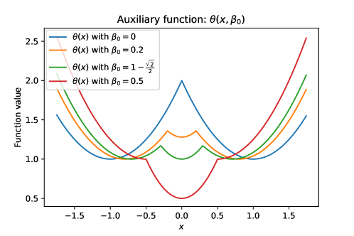
θ​(x,Ξ²0)=πœƒπ‘₯subscript𝛽0absent\displaystyle\theta(x,\beta_{0})= (max⁑{0,x+Ξ²0}βˆ’1)2+(max⁑{0,βˆ’x+Ξ²0}βˆ’1)2superscript0π‘₯subscript𝛽012superscript0π‘₯subscript𝛽012\displaystyle(\max\{0,x+\beta_{0}\}-1)^{2}+(\max\{0,-x+\beta_{0}\}-1)^{2}

(See Figure 4).

Refer to caption
Figure 4: Function θ​(x,Ξ²0)πœƒπ‘₯subscript𝛽0\theta(x,\beta_{0})

For a fixed xπ‘₯x, let g​(Ξ²0)=minx⁑θ​(x,Ξ²0)𝑔subscript𝛽0subscriptπ‘₯πœƒπ‘₯subscript𝛽0g(\beta_{0})=\min_{x}\theta(x,\beta_{0}). We construct our affine One-Node-ReLU problem as follows:

minΞ²,Ξ²0βˆˆβ„p+1⁑(max⁑{0,βˆ‘i=1pai​βi+Ξ²0}βˆ’12β€‹βˆ‘i=1pai)2+(max⁑{0,βˆ‘i=1p2β‹…ai​βi+Ξ²0}βˆ’βˆ‘i=1pai)2⏟=⁣:τ​(Ξ²,Ξ²0)subscript𝛽subscript𝛽0superscriptℝ𝑝1subscript⏟superscript0superscriptsubscript𝑖1𝑝subscriptπ‘Žπ‘–subscript𝛽𝑖subscript𝛽012superscriptsubscript𝑖1𝑝subscriptπ‘Žπ‘–2superscript0superscriptsubscript𝑖1𝑝⋅2subscriptπ‘Žπ‘–subscript𝛽𝑖subscript𝛽0superscriptsubscript𝑖1𝑝subscriptπ‘Žπ‘–2:absentπœπ›½subscript𝛽0\displaystyle\min_{\beta,\beta_{0}\in\mathbb{R}^{p+1}}\underbrace{\bigg{(}\max\bigg{\{}0,\sum_{i=1}^{p}a_{i}\beta_{i}+\beta_{0}\bigg{\}}-\frac{1}{2}\sum_{i=1}^{p}a_{i}\bigg{)}^{2}+\bigg{(}\max\bigg{\{}0,\sum_{i=1}^{p}2\cdot a_{i}\beta_{i}+\beta_{0}\bigg{\}}-\sum_{i=1}^{p}a_{i}\bigg{)}^{2}}_{=:\tau(\beta,\beta_{0})}
+βˆ‘i=1pθ​(ejβŠ€β€‹Ξ²,Ξ²0)+(max⁑{0,Ξ²0}+10​p)2.superscriptsubscript𝑖1π‘πœƒsuperscriptsubscript𝑒𝑗top𝛽subscript𝛽0superscript0subscript𝛽010𝑝2\displaystyle+\sum_{i=1}^{p}\theta(e_{j}^{\top}\beta,\beta_{0})+\bigg{(}\max\{0,\beta_{0}\}+10p\bigg{)}^{2}. (ReLU)

Observe that solving (ReLU) is equivalent to training a One-Node-ReLU where the data samples are:

  1. 1.

    X1=[a1,…,ap]subscript𝑋1subscriptπ‘Ž1…subscriptπ‘Žπ‘X_{1}=[a_{1},\dots,a_{p}], Y1=12β€‹βˆ‘i=1paisubscriptπ‘Œ112superscriptsubscript𝑖1𝑝subscriptπ‘Žπ‘–Y_{1}=\frac{1}{2}\sum_{i=1}^{p}a_{i}

  2. 2.

    X2=[2β‹…a1,…,2β‹…ap]subscript𝑋2β‹…2subscriptπ‘Ž1…⋅2subscriptπ‘Žπ‘X_{2}=[2\cdot a_{1},\dots,2\cdot a_{p}], Y1=βˆ‘i=1paisubscriptπ‘Œ1superscriptsubscript𝑖1𝑝subscriptπ‘Žπ‘–Y_{1}=\sum_{i=1}^{p}a_{i}

  3. 3.

    X2​i+1=eisubscript𝑋2𝑖1subscript𝑒𝑖X_{2i+1}=e_{i}, Y2​i+1=1subscriptπ‘Œ2𝑖11Y_{2i+1}=1, X2​i+2=βˆ’eisubscript𝑋2𝑖2subscript𝑒𝑖X_{2i+2}=-e_{i}, Y2​i+2=1subscriptπ‘Œ2𝑖21Y_{2i+2}=1 for i∈{1,…,p}𝑖1…𝑝i\in\{1,\dots,p\}.

  4. 4.

    X2​p+3=0subscript𝑋2𝑝30X_{2p+3}=0, Y2​p+3=10​psubscriptπ‘Œ2𝑝310𝑝Y_{2p+3}=10p.

Now we verify TheoremΒ 1 by showing that the {Β±1}βˆ’limit-fromplus-or-minus1\{\pm 1\}-subset sum problem iff the training error in solving (ReLU) is p+100​p2𝑝100superscript𝑝2p+100p^{2}.

Thus

  • β€’

    Suppose the {Β±1}βˆ’limit-fromplus-or-minus1\{\pm 1\}-subset sum problem with non-negative parameters a1,…,apsubscriptπ‘Ž1…subscriptπ‘Žπ‘a_{1},\ldots,a_{p} has a feasible solution x∈{Β±1}pπ‘₯superscriptplus-or-minus1𝑝x\in\{\pm 1\}^{p} such that βˆ‘i=1pai​xi=12β€‹βˆ‘i=1paisuperscriptsubscript𝑖1𝑝subscriptπ‘Žπ‘–subscriptπ‘₯𝑖12superscriptsubscript𝑖1𝑝subscriptπ‘Žπ‘–\sum_{i=1}^{p}a_{i}x_{i}=\frac{1}{2}\sum_{i=1}^{p}a_{i}. Let Ξ²=x𝛽π‘₯\beta=x and Ξ²0=0subscript𝛽00\beta_{0}=0, we have that the objective function value of (ReLU) is p+100​p2𝑝100superscript𝑝2p+100p^{2}.

  • β€’

    Suppose the {Β±1}βˆ’limit-fromplus-or-minus1\{\pm 1\}-subset sum problem does not have a feasible solution. Let Ξ²,Ξ²0𝛽subscript𝛽0\beta,\beta_{0} be the optimal solution to (ReLU). Then, observe that

    g​(Ξ²0)={2​β02βˆ’4​β0+2Β when ​β0β‰₯1βˆ’221Β when ​β0≀1βˆ’22(≀12).𝑔subscript𝛽0cases2superscriptsubscript𝛽024subscript𝛽02Β whenΒ subscript𝛽0122missing-subexpression1Β whenΒ subscript𝛽0annotated122absent12missing-subexpression\displaystyle g(\beta_{0})=\left\{\begin{array}[]{lll}2\beta_{0}^{2}-4\beta_{0}+2&\text{ when }\beta_{0}\geq 1-\frac{\sqrt{2}}{2}\\ 1&\text{ when }\beta_{0}\leq 1-\frac{\sqrt{2}}{2}\leavevmode\nobreak\ (\leq\frac{1}{2})\end{array}\right..

    We consider four cases:

    1. 1.

      Ξ²0β‰₯1βˆ’22subscript𝛽0122\beta_{0}\geq 1-\frac{\sqrt{2}}{2}: In this case τ​(Ξ²,Ξ²0)+pβ‹…g​(Ξ²0)+(max⁑{0,Ξ²0}+10​p)2β‰₯0+p​(2​β02βˆ’4​β0+2)+(Ξ²0+10​p)2=(2​p+1)​β02+16​p​β0+2​p+100​p2>p+100​p2πœπ›½subscript𝛽0⋅𝑝𝑔subscript𝛽0superscript0subscript𝛽010𝑝20𝑝2superscriptsubscript𝛽024subscript𝛽02superscriptsubscript𝛽010𝑝22𝑝1superscriptsubscript𝛽0216𝑝subscript𝛽02𝑝100superscript𝑝2𝑝100superscript𝑝2\tau(\beta,\beta_{0})+p\cdot g(\beta_{0})+(\max\{0,\beta_{0}\}+10p)^{2}\geq 0+p(2\beta_{0}^{2}-4\beta_{0}+2)+(\beta_{0}+10p)^{2}=(2p+1)\beta_{0}^{2}+16p\beta_{0}+2p+100p^{2}>p+100p^{2}.

    2. 2.

      0<Ξ²0≀1βˆ’220subscript𝛽01220<\beta_{0}\leq 1-\frac{\sqrt{2}}{2}: In this case τ​(Ξ²,Ξ²0)+pβ‹…g​(Ξ²0)+(max⁑{0,Ξ²0}+10​p)2β‰₯0+pβˆ—1+(Ξ²0+10​p)2>p+100​p2πœπ›½subscript𝛽0⋅𝑝𝑔subscript𝛽0superscript0subscript𝛽010𝑝20𝑝1superscriptsubscript𝛽010𝑝2𝑝100superscript𝑝2\tau(\beta,\beta_{0})+p\cdot g(\beta_{0})+(\max\{0,\beta_{0}\}+10p)^{2}\geq 0+p*1+(\beta_{0}+10p)^{2}>p+100p^{2}.

    3. 3.

      Ξ²0<0subscript𝛽00\beta_{0}<0: Note that 12β€‹βˆ‘i=1pai>012superscriptsubscript𝑖1𝑝subscriptπ‘Žπ‘–0\frac{1}{2}\sum_{i=1}^{p}a_{i}>0 and therefore τ​(Ξ²,Ξ²0)=0πœπ›½subscript𝛽00\tau(\beta,\beta_{0})=0 iff Ξ²0=0subscript𝛽00\beta_{0}=0. In particular in this case τ​(Ξ²,Ξ²0)>0πœπ›½subscript𝛽00\tau(\beta,\beta_{0})>0. Therefore, we have τ​(Ξ²,Ξ²0)+pβ‹…g​(Ξ²0)+(max⁑{0,Ξ²0}+10​p)2>0+pβ‹…1+100​p2πœπ›½subscript𝛽0⋅𝑝𝑔subscript𝛽0superscript0subscript𝛽010𝑝20⋅𝑝1100superscript𝑝2\tau(\beta,\beta_{0})+p\cdot g(\beta_{0})+(\max\{0,\beta_{0}\}+10p)^{2}>0+p\cdot 1+100p^{2}.

    4. 4.

      Ξ²0=0subscript𝛽00\beta_{0}=0: In this case, observe that

      τ​(Ξ²,Ξ²0)+βˆ‘i=1pθ​(ejβŠ€β€‹Ξ²,Ξ²0)+(max⁑{0,Ξ²0}+10​p)2β‰₯0+pβ‹…1+100​p2.πœπ›½subscript𝛽0superscriptsubscript𝑖1π‘πœƒsuperscriptsubscript𝑒𝑗top𝛽subscript𝛽0superscript0subscript𝛽010𝑝20⋅𝑝1100superscript𝑝2\tau(\beta,\beta_{0})+\sum_{i=1}^{p}\theta(e_{j}^{\top}\beta,\beta_{0})+(\max\{0,\beta_{0}\}+10p)^{2}\geq 0+p\cdot 1+100p^{2}.

      However, for equality to hold in the above inequality, we must have θ​(ejβŠ€β€‹Ξ²,Ξ²0)=1πœƒsuperscriptsubscript𝑒𝑗top𝛽subscript𝛽01\theta(e_{j}^{\top}\beta,\beta_{0})=1 for j∈[p]𝑗delimited-[]𝑝j\in[p] and τ​(Ξ²,Ξ²0)=0πœπ›½subscript𝛽00\tau(\beta,\beta_{0})=0, which implies we must have Ξ²j∈{βˆ’1,1}subscript𝛽𝑗11\beta_{j}\in\{-1,1\} and βˆ‘i=1pai​βi=12β€‹βˆ‘i=1paisuperscriptsubscript𝑖1𝑝subscriptπ‘Žπ‘–subscript𝛽𝑖12superscriptsubscript𝑖1𝑝subscriptπ‘Žπ‘–\sum_{i=1}^{p}a_{i}\beta_{i}=\frac{1}{2}\sum_{i=1}^{p}a_{i}. However since there is no solution to the {Β±1}βˆ’limit-fromplus-or-minus1\{\pm 1\}-subset sum problem, we obtain that τ​(Ξ²,Ξ²0)+βˆ‘i=1pθ​(ejβŠ€β€‹Ξ²,Ξ²0)+(max⁑{0,Ξ²0}+10​p)2>0+pβ‹…1+100​p2.πœπ›½subscript𝛽0superscriptsubscript𝑖1π‘πœƒsuperscriptsubscript𝑒𝑗top𝛽subscript𝛽0superscript0subscript𝛽010𝑝20⋅𝑝1100superscript𝑝2\tau(\beta,\beta_{0})+\sum_{i=1}^{p}\theta(e_{j}^{\top}\beta,\beta_{0})+(\max\{0,\beta_{0}\}+10p)^{2}>0+p\cdot 1+100p^{2}.

5.3 Proof of Proposition 2

Proof.

Re-written

β€–max⁑{𝟎,XβŠ€β€‹Ξ²+Ξ²0β€‹πŸ}βˆ’Yβ€–22=βˆ‘i=1m(max⁑{0,XiβŠ€β€‹Ξ²+Ξ²0}βˆ’Yi)2+ϕ​(Ξ²,Ξ²0).superscriptsubscriptnorm0superscript𝑋top𝛽subscript𝛽01π‘Œ22superscriptsubscript𝑖1π‘šsuperscript0superscriptsubscript𝑋𝑖top𝛽subscript𝛽0subscriptπ‘Œπ‘–2italic-ϕ𝛽subscript𝛽0\|\max\{\mathbf{0},X^{\top}\beta+\beta_{0}\mathbf{1}\}-Y\|_{2}^{2}=\sum_{i=1}^{m}(\max\{0,X_{i}^{\top}\beta+\beta_{0}\}-Y_{i})^{2}+\phi(\beta,\beta_{0}).

Note that Yi>0subscriptπ‘Œπ‘–0Y_{i}>0 for all i∈[m]𝑖delimited-[]π‘ši\in[m], then we have:

(max⁑{0,XiβŠ€β€‹Ξ²+Ξ²0}βˆ’Yi)2≀(XiβŠ€β€‹Ξ²+Ξ²0βˆ’Yi)2superscript0superscriptsubscript𝑋𝑖top𝛽subscript𝛽0subscriptπ‘Œπ‘–2superscriptsuperscriptsubscript𝑋𝑖top𝛽subscript𝛽0subscriptπ‘Œπ‘–2\displaystyle(\max\{0,X_{i}^{\top}\beta+\beta_{0}\}-Y_{i})^{2}\leq(X_{i}^{\top}\beta+\beta_{0}-Y_{i})^{2}
(max⁑{0,XiβŠ€β€‹Ξ²+Ξ²0}βˆ’Yi)2≀σ​(XiβŠ€β€‹Ξ²+Ξ²0,Yi)superscript0superscriptsubscript𝑋𝑖top𝛽subscript𝛽0subscriptπ‘Œπ‘–2𝜎superscriptsubscript𝑋𝑖top𝛽subscript𝛽0subscriptπ‘Œπ‘–\displaystyle(\max\{0,X_{i}^{\top}\beta+\beta_{0}\}-Y_{i})^{2}\leq\sigma(X_{i}^{\top}\beta+\beta_{0},Y_{i})

holds for all i∈[m]𝑖delimited-[]π‘ši\in[m]. Since for any IβŠ†[m]𝐼delimited-[]π‘šI\subseteq[m]

βˆ‘i=1m(max⁑{0,XiβŠ€β€‹Ξ²+Ξ²0}βˆ’Yi)2+ϕ​(Ξ²,Ξ²0)β‰€βˆ‘i∈I(XiβŠ€β€‹Ξ²+Ξ²0βˆ’Yi)2+βˆ‘i∈[m]\Iσ​(XiβŠ€β€‹Ξ²+Ξ²0,Yi)+ϕ​(Ξ²,Ξ²0),superscriptsubscript𝑖1π‘šsuperscript0superscriptsubscript𝑋𝑖top𝛽subscript𝛽0subscriptπ‘Œπ‘–2italic-ϕ𝛽subscript𝛽0subscript𝑖𝐼superscriptsuperscriptsubscript𝑋𝑖top𝛽subscript𝛽0subscriptπ‘Œπ‘–2subscript𝑖\delimited-[]π‘šπΌπœŽsuperscriptsubscript𝑋𝑖top𝛽subscript𝛽0subscriptπ‘Œπ‘–italic-ϕ𝛽subscript𝛽0\sum_{i=1}^{m}(\max\{0,X_{i}^{\top}\beta+\beta_{0}\}-Y_{i})^{2}+\phi(\beta,\beta_{0})\leq\sum_{i\in I}(X_{i}^{\top}\beta+\beta_{0}-Y_{i})^{2}+\sum_{i\in[m]\backslash I}\sigma(X_{i}^{\top}\beta+\beta_{0},Y_{i})+\phi(\beta,\beta_{0}),

then taking minimum on both side implies min(Ξ²,Ξ²0)βˆˆβ„p×ℝ⁑‖max⁑{𝟎,XβŠ€β€‹Ξ²+Ξ²0β€‹πŸ}βˆ’Yβ€–22≀zσ​(I)subscript𝛽subscript𝛽0superscriptℝ𝑝ℝsuperscriptsubscriptnorm0superscript𝑋top𝛽subscript𝛽01π‘Œ22superscriptπ‘§πœŽπΌ\min_{(\beta,\beta_{0})\in\mathbb{R}^{p}\times\mathbb{R}}\|\max\{\mathbf{0},X^{\top}\beta+\beta_{0}\mathbf{1}\}-Y\|_{2}^{2}\leq z^{\sigma}(I).

Moreover, recall IOPTsuperscript𝐼OPTI^{\text{OPT}} is the active set corresponding to a global optimal solution (Ξ²OPT,Ξ²0OPT)superscript𝛽OPTsubscriptsuperscript𝛽OPT0(\beta^{\text{OPT}},\beta^{\text{OPT}}_{0}) as defined above. We have:

zσ​(IOPT)≀superscriptπ‘§πœŽsuperscript𝐼OPTabsent\displaystyle z^{\sigma}(I^{\text{OPT}})\leq βˆ‘i∈IOPT(XiβŠ€β€‹Ξ²OPT+Ξ²0OPT⏟β‰₯0βˆ’Yi)2+βˆ‘i∈[m]\IOPTσ​(XiβŠ€β€‹Ξ²OPT+Ξ²0OPT⏟<0,Yi)+ϕ​(Ξ²OPT,Ξ²0OPT)subscript𝑖superscript𝐼OPTsuperscriptsubscript⏟superscriptsubscript𝑋𝑖topsuperscript𝛽OPTsubscriptsuperscript𝛽OPT0absent0subscriptπ‘Œπ‘–2subscript𝑖\delimited-[]π‘šsuperscript𝐼OPT𝜎subscript⏟superscriptsubscript𝑋𝑖topsuperscript𝛽OPTsubscriptsuperscript𝛽OPT0absent0subscriptπ‘Œπ‘–italic-Ο•superscript𝛽OPTsubscriptsuperscript𝛽OPT0\displaystyle\leavevmode\nobreak\ \sum_{i\in I^{\text{OPT}}}(\underbrace{X_{i}^{\top}\beta^{\text{OPT}}+\beta^{\text{OPT}}_{0}}_{\geq 0}-Y_{i})^{2}+\sum_{i\in[m]\backslash I^{\text{OPT}}}\sigma(\underbrace{X_{i}^{\top}\beta^{\text{OPT}}+\beta^{\text{OPT}}_{0}}_{<0},Y_{i})+\phi(\beta^{\text{OPT}},\beta^{\text{OPT}}_{0})
=\displaystyle= βˆ‘i∈IOPT(XiβŠ€β€‹Ξ²OPT+Ξ²0OPTβˆ’Yi)2+βˆ‘i∈[m]\IOPTYi2+ϕ​(Ξ²OPT,Ξ²0OPT)subscript𝑖superscript𝐼OPTsuperscriptsuperscriptsubscript𝑋𝑖topsuperscript𝛽OPTsubscriptsuperscript𝛽OPT0subscriptπ‘Œπ‘–2subscript𝑖\delimited-[]π‘šsuperscript𝐼OPTsuperscriptsubscriptπ‘Œπ‘–2italic-Ο•superscript𝛽OPTsubscriptsuperscript𝛽OPT0\displaystyle\leavevmode\nobreak\ \sum_{i\in I^{\text{OPT}}}(X_{i}^{\top}\beta^{\text{OPT}}+\beta^{\text{OPT}}_{0}-Y_{i})^{2}+\sum_{i\in[m]\backslash I^{\text{OPT}}}Y_{i}^{2}+\phi(\beta^{\text{OPT}},\beta^{\text{OPT}}_{0})
=\displaystyle= zOPT.superscript𝑧OPT\displaystyle\leavevmode\nobreak\ z^{\text{OPT}}.

Combine with zOPT=β€–max⁑{𝟎,XβŠ€β€‹Ξ²+Ξ²0β€‹πŸ}βˆ’Yβ€–22≀zσ​(IOPT)superscript𝑧OPTsuperscriptsubscriptnorm0superscript𝑋top𝛽subscript𝛽01π‘Œ22superscriptπ‘§πœŽsuperscript𝐼OPTz^{\text{OPT}}=\|\max\{\mathbf{0},X^{\top}\beta+\beta_{0}\mathbf{1}\}-Y\|_{2}^{2}\leq z^{\sigma}(I^{\text{OPT}}), we have zOPT=zσ​(IOPT)superscript𝑧OPTsuperscriptπ‘§πœŽsuperscript𝐼OPTz^{\text{OPT}}=z^{\sigma}(I^{\text{OPT}}). ∎

5.4 Proof of Proposition 2

Proof.

Recall that (Ξ²OPT,Ξ²0OPT)superscript𝛽OPTsubscriptsuperscript𝛽OPT0(\beta^{\text{OPT}},\beta^{\text{OPT}}_{0}) is a global optimal solution, and zOPTsuperscript𝑧OPTz^{\text{OPT}} is the global optimal value of One-Node-ReLU. Let IOPT={i:XiβŠ€β€‹Ξ²OPT+Ξ²0OPT>0}βŠ†[m]superscript𝐼OPTconditional-set𝑖superscriptsubscript𝑋𝑖topsuperscript𝛽OPTsubscriptsuperscript𝛽OPT00delimited-[]π‘šI^{\text{OPT}}=\left\{i:X_{i}^{\top}\beta^{\text{OPT}}+\beta^{\text{OPT}}_{0}>0\right\}\subseteq[m] be the active set corresponds to (Ξ²OPT,Ξ²0OPT)superscript𝛽OPTsubscriptsuperscript𝛽OPT0(\beta^{\text{OPT}},\beta^{\text{OPT}}_{0}). Based on the input condition of AlgorithmΒ 1, the response samples {Yi}subscriptπ‘Œπ‘–\{Y_{i}\} satisfies:

0<Y1≀Y2≀…≀Ym.0subscriptπ‘Œ1subscriptπ‘Œ2…subscriptπ‘Œπ‘š\displaystyle 0<Y_{1}\leq Y_{2}\leq\ldots\leq Y_{m}.

Given kπ‘˜k as a predefined integral parameter, pick kπ‘˜k indices i1,i2,…,iksubscript𝑖1subscript𝑖2…subscriptπ‘–π‘˜i_{1},i_{2},\ldots,i_{k} such that 0≀i1<…<ik≀m0subscript𝑖1…subscriptπ‘–π‘˜π‘š0\leq i_{1}<\ldots<i_{k}\leq m, from AlgorithmΒ 1, we have:

[m]\I^:=assign\delimited-[]π‘š^𝐼absent\displaystyle[m]\backslash\hat{I}:= {1,…,i1}βˆͺ(⋃ℓ=2k{iβ„“})1…subscript𝑖1superscriptsubscriptβ„“2π‘˜subscript𝑖ℓ\displaystyle\{1,\ldots,i_{1}\}\cup\left(\bigcup_{\ell=2}^{k}\{i_{\ell}\}\right) be our inactive set,be our inactive set\displaystyle\text{ be our inactive set},
I^:=assign^𝐼absent\displaystyle\hat{I}:= (⋃ℓ=1kβˆ’1{iβ„“+1,…,iβ„“+1βˆ’1})βˆͺ{ik+1,…,m}superscriptsubscriptβ„“1π‘˜1subscript𝑖ℓ1…subscript𝑖ℓ11subscriptπ‘–π‘˜1β€¦π‘š\displaystyle\left(\bigcup_{\ell=1}^{k-1}\left\{i_{\ell}+1,\ldots,i_{\ell+1}-1\right\}\right)\cup\{i_{k}+1,\ldots,m\} be our active set.

Suppose IOPTsuperscript𝐼OPTI^{\text{OPT}} is of size |IOPT|β‰₯mβˆ’k+1superscript𝐼OPTπ‘šπ‘˜1|I^{\text{OPT}}|\geq m-k+1, let {sβ„“}β„“=1psuperscriptsubscriptsubscript𝑠ℓℓ1𝑝\{s_{\ell}\}_{\ell=1}^{p} with p≀kβˆ’1π‘π‘˜1p\leq k-1 be the set of increasingly-sorted indices that are not in IOPTsuperscript𝐼OPTI^{\text{OPT}}. Let j=p+1≀k𝑗𝑝1π‘˜j=p+1\leq k, set i1=0subscript𝑖10i_{1}=0, iβ„“=sβ„“βˆ’1,subscript𝑖ℓsubscript𝑠ℓ1i_{\ell}=s_{\ell-1}, for all β„“=2,…,jβ„“2…𝑗\ell=2,\ldots,j. Then we see that AlgorithmΒ 1 would discover the optimal solution and thus solve the One-Node-ReLU problem exactly.

Therefore, henceforth we assume that |IOPT|≀mβˆ’ksuperscript𝐼OPTπ‘šπ‘˜|I^{\text{OPT}}|\leq m-k.

Now pick i1,…,iksubscript𝑖1…subscriptπ‘–π‘˜i_{1},\ldots,i_{k} as the largest increasingly-sorted indices that not in IOPTsuperscript𝐼OPTI^{\text{OPT}}. Therefore we have: (1) I^βŠ†IOPT^𝐼superscript𝐼OPT\hat{I}\subseteq I^{\text{OPT}}, (2) ⋃ℓ=1k{iβ„“}βŠ†[m]\IOPTsuperscriptsubscriptβ„“1π‘˜subscript𝑖ℓ\delimited-[]π‘šsuperscript𝐼OPT\bigcup_{\ell=1}^{k}\{i_{\ell}\}\subseteq[m]\backslash I^{\text{OPT}}, and (3) ikβˆ’1∈IOPT​ if ​ikβˆ’1β‰ ikβˆ’1subscriptπ‘–π‘˜1superscript𝐼OPTΒ ifΒ subscriptπ‘–π‘˜1subscriptπ‘–π‘˜1i_{k}-1\in I^{\text{OPT}}\text{ if }i_{k-1}\neq i_{k}-1, these three conditions further implies that

IOPT\I^βŠ†{1,…,i1βˆ’1}.\superscript𝐼OPT^𝐼1…subscript𝑖11I^{\text{OPT}}\backslash\hat{I}\subseteq\{1,\ldots,i_{1}-1\}.

Since the approximation algorithm examines this solution, we will use this β€œsolution” to obtain an upper bound on the quality of solution produced by the Algorithm.

Thus the objective value zσ​(I^)superscriptπ‘§πœŽ^𝐼z^{\sigma}(\hat{I}) is further upper bounded as follows:

zσ​(I^)=superscriptπ‘§πœŽ^𝐼absent\displaystyle z^{\sigma}(\hat{I})= min(Ξ²,Ξ²0)βˆˆβ„pΓ—β„β€‹βˆ‘i∈I^(XiβŠ€β€‹Ξ²+Ξ²0βˆ’Yi)2+βˆ‘i∈[m]\I^σ​(XiβŠ€β€‹Ξ²+Ξ²0,Yi)+ϕ​(Ξ²,Ξ²0)subscript𝛽subscript𝛽0superscriptℝ𝑝ℝsubscript𝑖^𝐼superscriptsuperscriptsubscript𝑋𝑖top𝛽subscript𝛽0subscriptπ‘Œπ‘–2subscript𝑖\delimited-[]π‘š^𝐼𝜎superscriptsubscript𝑋𝑖top𝛽subscript𝛽0subscriptπ‘Œπ‘–italic-ϕ𝛽subscript𝛽0\displaystyle\leavevmode\nobreak\ \min_{(\beta,\beta_{0})\in\mathbb{R}^{p}\times\mathbb{R}}\sum_{i\in\hat{I}}(X_{i}^{\top}\beta+\beta_{0}-Y_{i})^{2}+\sum_{i\in[m]\backslash\hat{I}}\sigma(X_{i}^{\top}\beta+\beta_{0},Y_{i})+\phi(\beta,\beta_{0})
≀\displaystyle\leq βˆ‘i∈I^(XiβŠ€β€‹Ξ²OPT+Ξ²0OPT⏟β‰₯0βˆ’Yi)2+βˆ‘i∈IOPT\I^σ​(XiβŠ€β€‹Ξ²OPT+Ξ²0OPT⏟β‰₯0,Yi)subscript𝑖^𝐼superscriptsubscript⏟superscriptsubscript𝑋𝑖topsuperscript𝛽OPTsubscriptsuperscript𝛽OPT0absent0subscriptπ‘Œπ‘–2subscript𝑖\superscript𝐼OPT^𝐼𝜎subscript⏟superscriptsubscript𝑋𝑖topsuperscript𝛽OPTsubscriptsuperscript𝛽OPT0absent0subscriptπ‘Œπ‘–\displaystyle\leavevmode\nobreak\ \sum_{i\in\hat{I}}(\underbrace{X_{i}^{\top}\beta^{\text{OPT}}+\beta^{\text{OPT}}_{0}}_{\geq 0}-Y_{i})^{2}+\sum_{i\in I^{\text{OPT}}\backslash\hat{I}}\sigma(\underbrace{X_{i}^{\top}\beta^{\text{OPT}}+\beta^{\text{OPT}}_{0}}_{\geq 0},Y_{i})
+βˆ‘i∈[m]\IOPTσ​(XiβŠ€β€‹Ξ²OPT+Ξ²0OPT⏟<0,Yi)+ϕ​(Ξ²OPT,Ξ²0OPT)subscript𝑖\delimited-[]π‘šsuperscript𝐼OPT𝜎subscript⏟superscriptsubscript𝑋𝑖topsuperscript𝛽OPTsubscriptsuperscript𝛽OPT0absent0subscriptπ‘Œπ‘–italic-Ο•superscript𝛽OPTsubscriptsuperscript𝛽OPT0\displaystyle\leavevmode\nobreak\ +\sum_{i\in[m]\backslash I^{\text{OPT}}}\sigma(\underbrace{X_{i}^{\top}\beta^{\text{OPT}}+\beta^{\text{OPT}}_{0}}_{<0},Y_{i})+\phi(\beta^{\text{OPT}},\beta^{\text{OPT}}_{0})
=\displaystyle= βˆ‘i∈I^(XiβŠ€β€‹Ξ²OPT+Ξ²0OPTβˆ’Yi)2+βˆ‘i∈IOPT\I^σ​(XiβŠ€β€‹Ξ²OPT+Ξ²0OPT,Yi)+βˆ‘i∈[m]\IOPTYi2+ϕ​(Ξ²OPT,Ξ²0OPT).subscript𝑖^𝐼superscriptsuperscriptsubscript𝑋𝑖topsuperscript𝛽OPTsubscriptsuperscript𝛽OPT0subscriptπ‘Œπ‘–2subscript𝑖\superscript𝐼OPT^𝐼𝜎superscriptsubscript𝑋𝑖topsuperscript𝛽OPTsubscriptsuperscript𝛽OPT0subscriptπ‘Œπ‘–subscript𝑖\delimited-[]π‘šsuperscript𝐼OPTsuperscriptsubscriptπ‘Œπ‘–2italic-Ο•superscript𝛽OPTsubscriptsuperscript𝛽OPT0\displaystyle\leavevmode\nobreak\ \sum_{i\in\hat{I}}(X_{i}^{\top}\beta^{\text{OPT}}+\beta^{\text{OPT}}_{0}-Y_{i})^{2}+\sum_{i\in I^{\text{OPT}}\backslash\hat{I}}\sigma(X_{i}^{\top}\beta^{\text{OPT}}+\beta^{\text{OPT}}_{0},Y_{i})+\sum_{i\in[m]\backslash I^{\text{OPT}}}Y_{i}^{2}+\phi(\beta^{\text{OPT}},\beta^{\text{OPT}}_{0}).

Split IOPT\I^\superscript𝐼OPT^𝐼I^{\text{OPT}}\backslash\hat{I} into the following two parts:

I~+:=assignsubscript~𝐼absent\displaystyle\tilde{I}_{+}:= {i∈IOPT\I^:XiβŠ€β€‹Ξ²OPT+Ξ²0OPT>2​Yi},conditional-set𝑖\superscript𝐼OPT^𝐼superscriptsubscript𝑋𝑖topsuperscript𝛽OPTsuperscriptsubscript𝛽0OPT2subscriptπ‘Œπ‘–\displaystyle\leavevmode\nobreak\ \left\{i\in I^{\text{OPT}}\backslash\hat{I}:X_{i}^{\top}\beta^{\text{OPT}}+\beta_{0}^{\text{OPT}}>2Y_{i}\right\},
I~βˆ’:=assignsubscript~𝐼absent\displaystyle\tilde{I}_{-}:= {i∈IOPT\I^:2​Yiβ‰₯XiβŠ€β€‹Ξ²OPT+Ξ²0OPTβ‰₯0},conditional-set𝑖\superscript𝐼OPT^𝐼2subscriptπ‘Œπ‘–superscriptsubscript𝑋𝑖topsuperscript𝛽OPTsuperscriptsubscript𝛽0OPT0\displaystyle\leavevmode\nobreak\ \left\{i\in I^{\text{OPT}}\backslash\hat{I}:2Y_{i}\geq X_{i}^{\top}\beta^{\text{OPT}}+\beta_{0}^{\text{OPT}}\geq 0\right\},

the second term of above equals to:

βˆ‘i∈IOPT\I^σ​(XiβŠ€β€‹Ξ²OPT+Ξ²0OPT,Yi)=βˆ‘i∈I~+(XiβŠ€β€‹Ξ²OPT+Ξ²0OPTβˆ’Yi)2+βˆ‘i∈I~βˆ’Yi2.subscript𝑖\superscript𝐼OPT^𝐼𝜎superscriptsubscript𝑋𝑖topsuperscript𝛽OPTsubscriptsuperscript𝛽OPT0subscriptπ‘Œπ‘–subscript𝑖subscript~𝐼superscriptsuperscriptsubscript𝑋𝑖topsuperscript𝛽OPTsuperscriptsubscript𝛽0OPTsubscriptπ‘Œπ‘–2subscript𝑖subscript~𝐼superscriptsubscriptπ‘Œπ‘–2\displaystyle\sum_{i\in I^{\text{OPT}}\backslash\hat{I}}\sigma(X_{i}^{\top}\beta^{\text{OPT}}+\beta^{\text{OPT}}_{0},Y_{i})=\sum_{i\in\tilde{I}_{+}}(X_{i}^{\top}\beta^{\text{OPT}}+\beta_{0}^{\text{OPT}}-Y_{i})^{2}+\sum_{i\in\tilde{I}_{-}}Y_{i}^{2}.

Therefore,

zσ​(I^)β‰€βˆ‘i∈I^βˆͺI~+(XiβŠ€β€‹Ξ²OPT+Ξ²0OPTβˆ’Yi)2+βˆ‘i∈I~βˆ’βˆͺ([m]\IOPT)Yi2+ϕ​(Ξ²OPT,Ξ²0OPT).superscriptπ‘§πœŽ^𝐼subscript𝑖^𝐼subscript~𝐼superscriptsuperscriptsubscript𝑋𝑖topsuperscript𝛽OPTsuperscriptsubscript𝛽0OPTsubscriptπ‘Œπ‘–2subscript𝑖subscript~𝐼\delimited-[]π‘šsuperscript𝐼OPTsuperscriptsubscriptπ‘Œπ‘–2italic-Ο•superscript𝛽OPTsuperscriptsubscript𝛽0OPT\displaystyle z^{\sigma}(\hat{I})\leq\sum_{i\in\hat{I}\cup\tilde{I}_{+}}(X_{i}^{\top}\beta^{\text{OPT}}+\beta_{0}^{\text{OPT}}-Y_{i})^{2}+\sum_{i\in\tilde{I}_{-}\cup\left([m]\backslash I^{\text{OPT}}\right)}Y_{i}^{2}+\phi(\beta^{\text{OPT}},\beta_{0}^{\text{OPT}}). (UB)

Since IOPT=I^βˆͺI~+βˆͺI~βˆ’superscript𝐼OPT^𝐼subscript~𝐼subscript~𝐼I^{\text{OPT}}=\hat{I}\cup\tilde{I}_{+}\cup\tilde{I}_{-}, then the global optimal value of One-Node-ReLU can be represented as

zOPT=superscript𝑧OPTabsent\displaystyle z^{\text{OPT}}= βˆ‘i∈IOPT(XiβŠ€β€‹Ξ²OPT+Ξ²0OPTβˆ’Yi)2+βˆ‘i∈[m]\IOPTYi2+ϕ​(Ξ²OPT,Ξ²0OPT)subscript𝑖superscript𝐼OPTsuperscriptsuperscriptsubscript𝑋𝑖topsuperscript𝛽OPTsuperscriptsubscript𝛽0OPTsubscriptπ‘Œπ‘–2subscript𝑖\delimited-[]π‘šsuperscript𝐼OPTsuperscriptsubscriptπ‘Œπ‘–2italic-Ο•superscript𝛽OPTsuperscriptsubscript𝛽0OPT\displaystyle\leavevmode\nobreak\ \sum_{i\in I^{\text{OPT}}}(X_{i}^{\top}\beta^{\text{OPT}}+\beta_{0}^{\text{OPT}}-Y_{i})^{2}+\sum_{i\in[m]\backslash I^{\text{OPT}}}Y_{i}^{2}+\phi(\beta^{\text{OPT}},\beta_{0}^{\text{OPT}})
=\displaystyle= βˆ‘i∈I^βˆͺI~+(XiβŠ€β€‹Ξ²OPT+Ξ²0OPTβˆ’Yi)2+βˆ‘i∈I~βˆ’(XiβŠ€β€‹Ξ²OPT+Ξ²0OPTβˆ’Yi)2+βˆ‘i∈[m]\IOPTYi2+ϕ​(Ξ²OPT,Ξ²0OPT).subscript𝑖^𝐼subscript~𝐼superscriptsuperscriptsubscript𝑋𝑖topsuperscript𝛽OPTsuperscriptsubscript𝛽0OPTsubscriptπ‘Œπ‘–2subscript𝑖subscript~𝐼superscriptsuperscriptsubscript𝑋𝑖topsuperscript𝛽OPTsuperscriptsubscript𝛽0OPTsubscriptπ‘Œπ‘–2subscript𝑖\delimited-[]π‘šsuperscript𝐼OPTsuperscriptsubscriptπ‘Œπ‘–2italic-Ο•superscript𝛽OPTsuperscriptsubscript𝛽0OPT\displaystyle\leavevmode\nobreak\ \sum_{i\in\hat{I}\cup\tilde{I}_{+}}(X_{i}^{\top}\beta^{\text{OPT}}+\beta_{0}^{\text{OPT}}-Y_{i})^{2}+\sum_{i\in\tilde{I}_{-}}(X_{i}^{\top}\beta^{\text{OPT}}+\beta_{0}^{\text{OPT}}-Y_{i})^{2}+\sum_{i\in[m]\backslash I^{\text{OPT}}}Y_{i}^{2}+\phi(\beta^{\text{OPT}},\beta_{0}^{\text{OPT}}).

Note {i1,…,ik}subscript𝑖1…subscriptπ‘–π‘˜\{i_{1},\ldots,i_{k}\} is a subset of [m]\IOPT\delimited-[]π‘šsuperscript𝐼OPT[m]\backslash I^{\text{OPT}} based on our choice i1,…,iksubscript𝑖1…subscriptπ‘–π‘˜i_{1},\ldots,i_{k}, then the term D𝐷D satisfies:

D:=βˆ‘i∈I^βˆͺI~+(XiβŠ€β€‹Ξ²OPT+Ξ²0OPTβˆ’Yi)2+βˆ‘i∈[m]\IOPTYi2+ϕ​(Ξ²OPT,Ξ²0OPT)β‰₯βˆ‘j=1kYij2.assign𝐷subscript𝑖^𝐼subscript~𝐼superscriptsuperscriptsubscript𝑋𝑖topsuperscript𝛽OPTsuperscriptsubscript𝛽0OPTsubscriptπ‘Œπ‘–2subscript𝑖\delimited-[]π‘šsuperscript𝐼OPTsuperscriptsubscriptπ‘Œπ‘–2italic-Ο•superscript𝛽OPTsuperscriptsubscript𝛽0OPTsuperscriptsubscript𝑗1π‘˜superscriptsubscriptπ‘Œsubscript𝑖𝑗2\displaystyle D:=\sum_{i\in\hat{I}\cup\tilde{I}_{+}}(X_{i}^{\top}\beta^{\text{OPT}}+\beta_{0}^{\text{OPT}}-Y_{i})^{2}+\sum_{i\in[m]\backslash I^{\text{OPT}}}Y_{i}^{2}+\phi(\beta^{\text{OPT}},\beta_{0}^{\text{OPT}})\geq\sum_{j=1}^{k}Y_{i_{j}}^{2}. (1)

Since UB and zOPTsuperscript𝑧OPTz^{\text{OPT}} can be represented as:

(UB):=assignUBabsent\displaystyle(\text{UB}):= D+βˆ‘i∈I~βˆ’Yi2𝐷subscript𝑖subscript~𝐼superscriptsubscriptπ‘Œπ‘–2\displaystyle\leavevmode\nobreak\ D+\sum_{i\in\tilde{I}_{-}}Y_{i}^{2}
zOPT:=assignsuperscript𝑧OPTabsent\displaystyle z^{\text{OPT}}:= D+βˆ‘i∈I~βˆ’(XiβŠ€β€‹Ξ²OPT+Ξ²0OPTβˆ’Yi)2𝐷subscript𝑖subscript~𝐼superscriptsuperscriptsubscript𝑋𝑖topsuperscript𝛽OPTsuperscriptsubscript𝛽0OPTsubscriptπ‘Œπ‘–2\displaystyle\leavevmode\nobreak\ D+\sum_{i\in\tilde{I}_{-}}(X_{i}^{\top}\beta^{\text{OPT}}+\beta_{0}^{\text{OPT}}-Y_{i})^{2}

then the approximation ratio ρ𝜌\rho guaranteed by Algorithm 1 is upper bounded as follows:

ρ:=zσ​(I^)zOPT≀(U​B)zOPT=D+βˆ‘i∈I~βˆ’Yi2D+βˆ‘i∈I~βˆ’(XiβŠ€β€‹Ξ²OPT+Ξ²0OPTβˆ’Yi)2≀D+βˆ‘i∈I~βˆ’Yi2D≀nkassign𝜌superscriptπ‘§πœŽ^𝐼superscript𝑧OPTπ‘ˆπ΅superscript𝑧OPT𝐷subscript𝑖subscript~𝐼superscriptsubscriptπ‘Œπ‘–2𝐷subscript𝑖subscript~𝐼superscriptsuperscriptsubscript𝑋𝑖topsuperscript𝛽OPTsuperscriptsubscript𝛽0OPTsubscriptπ‘Œπ‘–2𝐷subscript𝑖subscript~𝐼superscriptsubscriptπ‘Œπ‘–2π·π‘›π‘˜\displaystyle\rho:=\frac{z^{\sigma}(\hat{I})}{z^{\text{OPT}}}\leq\frac{(UB)}{z^{\text{OPT}}}=\frac{D+\sum_{i\in\tilde{I}_{-}}Y_{i}^{2}}{D+\sum_{i\in\tilde{I}_{-}}(X_{i}^{\top}\beta^{\text{OPT}}+\beta_{0}^{\text{OPT}}-Y_{i})^{2}}\leq\frac{D+\sum_{i\in\tilde{I}_{-}}Y_{i}^{2}}{D}\leq\frac{n}{k}

where the final inequality holds because of the following: with {Yi}i=1msuperscriptsubscriptsubscriptπ‘Œπ‘–π‘–1π‘š\{Y_{i}\}_{i=1}^{m} increasingly-sorted, the term βˆ‘i∈I~βˆ’Yi2subscript𝑖subscript~𝐼superscriptsubscriptπ‘Œπ‘–2\sum_{i\in\tilde{I}_{-}}Y_{i}^{2} can be upper bounded by

βˆ‘i∈I~βˆ’Yi2≀subscript𝑖subscript~𝐼superscriptsubscriptπ‘Œπ‘–2absent\displaystyle\sum_{i\in\tilde{I}_{-}}Y_{i}^{2}\leq |I~βˆ’|β‹…Yi12β‹…subscript~𝐼superscriptsubscriptπ‘Œsubscript𝑖12\displaystyle\leavevmode\nobreak\ |\tilde{I}_{-}|\cdot Y_{i_{1}}^{2} by ​I~βˆ’βŠ†IOPT\I^βŠ†{1,…,i1βˆ’1},byΒ subscript~𝐼\superscript𝐼OPT^𝐼1…subscript𝑖11\displaystyle\text{ by }\tilde{I}_{-}\subseteq I^{\text{OPT}}\backslash\hat{I}\subseteq\{1,\ldots,i_{1}-1\},
≀\displaystyle\leq |I~βˆ’|kβ‹…βˆ‘j=1kYij2β‹…subscript~πΌπ‘˜superscriptsubscript𝑗1π‘˜superscriptsubscriptπ‘Œsubscript𝑖𝑗2\displaystyle\leavevmode\nobreak\ \frac{|\tilde{I}_{-}|}{k}\cdot\sum_{j=1}^{k}Y_{i_{j}}^{2} by ​Yijβ‰₯Yi1​ for all ​j=1,…,k,formulae-sequencebyΒ subscriptπ‘Œsubscript𝑖𝑗subscriptπ‘Œsubscript𝑖1Β for all 𝑗1β€¦π‘˜\displaystyle\text{ by }Y_{i_{j}}\geq Y_{i_{1}}\text{ for all }j=1,\ldots,k,
≀\displaystyle\leq |I~βˆ’|kβ‹…Dβ‹…subscript~πΌπ‘˜π·\displaystyle\leavevmode\nobreak\ \frac{|\tilde{I}_{-}|}{k}\cdot D by previous inequality of ​D,by previous inequality of 𝐷\displaystyle\text{ by previous inequality of }D,
≀\displaystyle\leq nβˆ’kkβ‹…Dβ‹…π‘›π‘˜π‘˜π·\displaystyle\leavevmode\nobreak\ \frac{n-k}{k}\cdot D by ​I~βˆ’βŠ†IOPT​ and ​|IOPT|≀mβˆ’k≀nβˆ’k,byΒ subscript~𝐼superscript𝐼OPTΒ andΒ superscript𝐼OPTπ‘šπ‘˜π‘›π‘˜\displaystyle\text{ by }\tilde{I}_{-}\subseteq I^{\text{OPT}}\text{ and }|I^{\text{OPT}}|\leq m-k\leq n-k,

then replacing βˆ‘i∈I~βˆ’Yi2subscript𝑖subscript~𝐼superscriptsubscriptπ‘Œπ‘–2\sum_{i\in\tilde{I}_{-}}Y_{i}^{2} by nβˆ’kkβ‹…Dβ‹…π‘›π‘˜π‘˜π·\frac{n-k}{k}\cdot D gives the final approximation ratio. ∎

5.5 Proof of TheoremΒ 3

We first verify PropositionΒ 3 and PropositionΒ 4. PropositionΒ 3 is a consequence of the following result:

Theorem 4 (Mickey, 1963).

Let g𝑔g be a function on π’³Γ—Ξ˜π’³Ξ˜\mathcal{X}\times\Theta where 𝒳𝒳\mathcal{X} is a Euclidean space and ΘΘ\Theta is a compact set of Euclidean space. Let g​(x,ΞΈ)𝑔π‘₯πœƒg(x,\theta) be a continuous function of ΞΈπœƒ\theta for each xβˆˆπ’³π‘₯𝒳x\in\mathcal{X} and a measurable function of xπ‘₯x for each ΞΈπœƒ\theta. Assume assume that |g​(x,ΞΈ)|≀h​(x)𝑔π‘₯πœƒβ„Žπ‘₯|g(x,\theta)|\leq h(x) for all xβˆˆπ’³π‘₯𝒳x\in\mathcal{X} and ΞΈβˆˆΞ˜πœƒΞ˜\theta\in\Theta, where hβ„Žh is integrable with respect to a probability distribution function F𝐹F on 𝒳𝒳\mathcal{X}. If x1,x2,…subscriptπ‘₯1subscriptπ‘₯2…x_{1},x_{2},\ldots is a random sample from F𝐹F then for almost every sequence {xt}subscriptπ‘₯𝑑\{x_{t}\}

1nβ€‹βˆ‘t=1ng​(xt,ΞΈ)β†’βˆ«g​(x,ΞΈ)​𝑑F​(x)β†’1𝑛superscriptsubscript𝑑1𝑛𝑔subscriptπ‘₯π‘‘πœƒπ‘”π‘₯πœƒdifferential-d𝐹π‘₯\displaystyle\frac{1}{n}\sum_{t=1}^{n}g(x_{t},\theta)\rightarrow\int g(x,\theta)dF(x)

uniformly for all ΞΈβˆˆΞ˜πœƒΞ˜\theta\in\Theta.

Proof.

of PropositionΒ 3 Let ψy​(XβŠ€β€‹Ξ²+Ξ²0,Y)subscriptπœ“π‘¦superscript𝑋top𝛽subscript𝛽0π‘Œ\psi_{y}(X^{\top}\beta+\beta_{0},Y) be defined as in PropositionΒ 3. Let 𝒳=ℝp×ℝ𝒳superscriptℝ𝑝ℝ\mathcal{X}=\mathbb{R}^{p}\times\mathbb{R} be a Euclidean space, and let ΘΘ\Theta be the same convex compact set in AssumptionΒ 1. We have ψy​(XβŠ€β€‹Ξ²+Ξ²0,Y)subscriptπœ“π‘¦superscript𝑋top𝛽subscript𝛽0π‘Œ\psi_{y}(X^{\top}\beta+\beta_{0},Y) is a continuous function of (Ξ²,Ξ²0)𝛽subscript𝛽0(\beta,\beta_{0}) for each (X,Y)βˆˆπ’³π‘‹π‘Œπ’³(X,Y)\in\mathcal{X} and a measurable function of (X,Y)π‘‹π‘Œ(X,Y) for each (Ξ²,Ξ²0)βˆˆΞ˜π›½subscript𝛽0Θ(\beta,\beta_{0})\in\Theta. Moreover, since ΘΘ\Theta is a convex compact set, then there exists a constant dΘ>0subscriptπ‘‘Ξ˜0d_{\Theta}>0 such that |ΞΈi|≀dΘsubscriptπœƒπ‘–subscriptπ‘‘Ξ˜|\theta_{i}|\leq d_{\Theta} for all i=0,1,…,p𝑖01…𝑝i=0,1,\ldots,p. Define function h​(X,Y)β„Žπ‘‹π‘Œh(X,Y) as

h​(X,Y)=2​(βˆ‘i=1p|[X]i|β‹…dΘ+dΘ)2+2​Y2β„Žπ‘‹π‘Œ2superscriptsuperscriptsubscript𝑖1𝑝⋅subscriptdelimited-[]𝑋𝑖subscriptπ‘‘Ξ˜subscriptπ‘‘Ξ˜22superscriptπ‘Œ2\displaystyle h(X,Y)=2\left(\sum_{i=1}^{p}|[X]_{i}|\cdot d_{\Theta}+d_{\Theta}\right)^{2}+2Y^{2}

where [X]isubscriptdelimited-[]𝑋𝑖[X]_{i} denotes the ithsuperscript𝑖thi^{\text{th}} component of X𝑋X for i=1,…,p𝑖1…𝑝i=1,\ldots,p. Thus we have h​(X,Y)β‰₯|ψy​(XβŠ€β€‹Ξ²+Ξ²0,Y)|β„Žπ‘‹π‘Œsubscriptπœ“π‘¦superscript𝑋top𝛽subscript𝛽0π‘Œh(X,Y)\geq|\psi_{y}(X^{\top}\beta+\beta_{0},Y)| holds for all (X,Y)βˆˆπ’³π‘‹π‘Œπ’³(X,Y)\in\mathcal{X} and (Ξ²,Ξ²0)βˆˆΞ˜π›½subscript𝛽0Θ(\beta,\beta_{0})\in\Theta, where h​(X,Y)β„Žπ‘‹π‘Œh(X,Y) is integrable with respect to a probability distribution π’©Γ—π’Ÿπ’©π’Ÿ\mathcal{N}\times\mathcal{D} on 𝒳𝒳\mathcal{X}. Since all the conditions in TheoremΒ 4 holds, PropositionΒ 3 holds. ∎

PropositionΒ 4 is a consequence of the following result:

Theorem 5 (Jennrich, 1969).

Under the statistical model: yt=f​(xt,ΞΈ0)+Ο΅tsubscript𝑦𝑑𝑓subscriptπ‘₯𝑑subscriptπœƒ0subscriptitalic-ϡ𝑑y_{t}=f(x_{t},\theta_{0})+\epsilon_{t} for all t=1,…,n𝑑1…𝑛t=1,\ldots,n when xtsubscriptπ‘₯𝑑x_{t} is ithsuperscript𝑖thi^{\text{th}} β€œfixed” input vector and {Ο΅t}subscriptitalic-ϡ𝑑\{\epsilon_{t}\} are i.i.d. distributed errors with zero mean and same finite unknown variance. Any vector ΞΈ^n∈Θsubscript^πœƒπ‘›Ξ˜\hat{\theta}_{n}\in\Theta which minimizes the residual sum of squares

Sn​(ΞΈ):=1nβ€‹βˆ‘t=1n(f​(xt,ΞΈ)βˆ’yt)2assignsubscriptπ‘†π‘›πœƒ1𝑛superscriptsubscript𝑑1𝑛superscript𝑓subscriptπ‘₯π‘‘πœƒsubscript𝑦𝑑2\displaystyle S_{n}(\theta):=\frac{1}{n}\sum_{t=1}^{n}(f(x_{t},\theta)-y_{t})^{2}

is said to be strongly consistent of ΞΈ0subscriptπœƒ0\theta_{0} (i.e., ΞΈ^nβ†’ΞΈ0β†’subscript^πœƒπ‘›subscriptπœƒ0\hat{\theta}_{n}\rightarrow\theta_{0} almost surely as nβ†’βˆžβ†’π‘›n\rightarrow\infty) under the following condition: Dn​(ΞΈ,ΞΈβ€²)subscriptπ·π‘›πœƒsuperscriptπœƒβ€²D_{n}(\theta,\theta^{\prime}) convergence uniformly to a continuous function D​(ΞΈ,ΞΈβ€²)π·πœƒsuperscriptπœƒβ€²D(\theta,\theta^{\prime}) and D​(ΞΈ,ΞΈ0)=0π·πœƒsubscriptπœƒ00D(\theta,\theta_{0})=0 if and only if ΞΈ=ΞΈ0πœƒsubscriptπœƒ0\theta=\theta_{0} where

Dn​(ΞΈ,ΞΈβ€²)=1nβ€‹βˆ‘t=1n(f​(xt,ΞΈ)βˆ’f​(xt,ΞΈβ€²))2.subscriptπ·π‘›πœƒsuperscriptπœƒβ€²1𝑛superscriptsubscript𝑑1𝑛superscript𝑓subscriptπ‘₯π‘‘πœƒπ‘“subscriptπ‘₯𝑑superscriptπœƒβ€²2\displaystyle D_{n}(\theta,\theta^{\prime})=\frac{1}{n}\sum_{t=1}^{n}(f(x_{t},\theta)-f(x_{t},\theta^{\prime}))^{2}.
Proof.

of PropositionΒ 4 Based on TheoremΒ 4, with the similar proof of PropositionΒ 3, we have:

1nβ€‹βˆ‘i=1n(max⁑{0,XiβŠ€β€‹Ξ²+Ξ²0}βˆ’max⁑{0,XiβŠ€β€‹Ξ²βˆ—+Ξ²0βˆ—})2⏟=⁣:Dn​((Ξ²,Ξ²0),(Ξ²βˆ—,Ξ²0βˆ—))subscript⏟1𝑛superscriptsubscript𝑖1𝑛superscript0superscriptsubscript𝑋𝑖top𝛽subscript𝛽00superscriptsubscript𝑋𝑖topsuperscriptπ›½βˆ—superscriptsubscript𝛽0βˆ—2:absentsubscript𝐷𝑛𝛽subscript𝛽0superscriptπ›½βˆ—subscriptsuperscriptπ›½βˆ—0\displaystyle\leavevmode\nobreak\ \underbrace{\frac{1}{n}\sum_{i=1}^{n}\left(\max\{0,X_{i}^{\top}\beta+\beta_{0}\}-\max\{0,X_{i}^{\top}\beta^{\ast}+\beta_{0}^{\ast}\}\right)^{2}}_{=:D_{n}((\beta,\beta_{0}),(\beta^{\ast},\beta^{\ast}_{0}))}
β†’β†’\displaystyle\rightarrow 𝔼XβˆΌπ’©,Ο΅βˆΌπ’Ÿβ€‹[(max⁑{0,XβŠ€β€‹Ξ²+Ξ²0}βˆ’max⁑{0,XβŠ€β€‹Ξ²βˆ—+Ξ²0βˆ—})2]⏟=⁣:D​((Ξ²,Ξ²0),(Ξ²βˆ—,Ξ²0βˆ—))subscript⏟subscript𝔼formulae-sequencesimilar-to𝑋𝒩similar-toitalic-Ο΅π’Ÿdelimited-[]superscript0superscript𝑋top𝛽subscript𝛽00superscript𝑋topsuperscriptπ›½βˆ—superscriptsubscript𝛽0βˆ—2:absent𝐷𝛽subscript𝛽0superscriptπ›½βˆ—subscriptsuperscriptπ›½βˆ—0\displaystyle\leavevmode\nobreak\ \underbrace{\mathbb{E}_{X\sim\mathcal{N},\epsilon\sim\mathcal{D}}\left[\left(\max\{0,X^{\top}\beta+\beta_{0}\}-\max\{0,X^{\top}\beta^{\ast}+\beta_{0}^{\ast}\}\right)^{2}\right]}_{=:D((\beta,\beta_{0}),(\beta^{\ast},\beta^{\ast}_{0}))}

uniformly for almost every sequence {Xi,Yi}subscript𝑋𝑖subscriptπ‘Œπ‘–\{X_{i},Y_{i}\}. Moreover, a direct consequence of the second property of distribution 𝒩𝒩\mathcal{N} (Unique Optimal Property) implies that D​((Ξ²,Ξ²0),(Ξ²βˆ—,Ξ²0βˆ—))=0𝐷𝛽subscript𝛽0superscriptπ›½βˆ—subscriptsuperscriptπ›½βˆ—00D((\beta,\beta_{0}),(\beta^{\ast},\beta^{\ast}_{0}))=0 if and only if (Ξ²,Ξ²0)=(Ξ²βˆ—,Ξ²0βˆ—)𝛽subscript𝛽0superscriptπ›½βˆ—subscriptsuperscriptπ›½βˆ—0(\beta,\beta_{0})=(\beta^{\ast},\beta^{\ast}_{0}). Thus, since all conditions of TheoremΒ 5 hold, PropositionΒ 4 holds. ∎

Proof.

of TheoremΒ 3 The optimal value of the asymptotic objective function from sorting algorithm can be upper bounded by replacing optimal solution with the true parameter Ξ²βˆ—superscriptπ›½βˆ—\beta^{\ast} as follows:

minΞ²βˆˆΞ˜β‘π”ΌXβˆΌπ’©,Ο΅βˆΌπ’Ÿβ€‹[ψy​(XβŠ€β€‹Ξ²+Ξ²0,Y)]≀𝔼XβˆΌπ’©,Ο΅βˆΌπ’Ÿβ€‹[ψy​(XβŠ€β€‹Ξ²βˆ—+Ξ²βˆ—,Y)],subscriptπ›½Ξ˜subscript𝔼formulae-sequencesimilar-to𝑋𝒩similar-toitalic-Ο΅π’Ÿdelimited-[]subscriptπœ“π‘¦superscript𝑋top𝛽subscript𝛽0π‘Œsubscript𝔼formulae-sequencesimilar-to𝑋𝒩similar-toitalic-Ο΅π’Ÿdelimited-[]subscriptπœ“π‘¦superscript𝑋topsuperscriptπ›½βˆ—superscriptπ›½βˆ—π‘Œ\displaystyle\min_{\beta\in\Theta}\mathbb{E}_{X\sim\mathcal{N},\epsilon\sim\mathcal{D}}[\psi_{y}(X^{\top}\beta+\beta_{0},Y)]\leq\mathbb{E}_{X\sim\mathcal{N},\epsilon\sim\mathcal{D}}[\psi_{y}(X^{\top}\beta^{\ast}+\beta^{\ast},Y)],

where 𝔼XβˆΌπ’©,Ο΅βˆΌπ’Ÿβ€‹[ψy​(XβŠ€β€‹Ξ²βˆ—+Ξ²0βˆ—,Y)]subscript𝔼formulae-sequencesimilar-to𝑋𝒩similar-toitalic-Ο΅π’Ÿdelimited-[]subscriptπœ“π‘¦superscript𝑋topsuperscriptπ›½βˆ—subscriptsuperscriptπ›½βˆ—0π‘Œ\mathbb{E}_{X\sim\mathcal{N},\epsilon\sim\mathcal{D}}[\psi_{y}(X^{\top}\beta^{\ast}+\beta^{\ast}_{0},Y)] can be split into the sum from (T1subscript𝑇1T_{1}) to (T7subscript𝑇7T_{7}):

𝔼XβˆΌπ’©,Ο΅βˆΌπ’Ÿβ€‹[ψy​(XβŠ€β€‹Ξ²βˆ—+Ξ²0βˆ—,Y)]subscript𝔼formulae-sequencesimilar-to𝑋𝒩similar-toitalic-Ο΅π’Ÿdelimited-[]subscriptπœ“π‘¦superscript𝑋topsuperscriptπ›½βˆ—subscriptsuperscriptπ›½βˆ—0π‘Œ\displaystyle\mathbb{E}_{X\sim\mathcal{N},\epsilon\sim\mathcal{D}}\big{[}\psi_{y}(X^{\top}\beta^{\ast}+\beta^{\ast}_{0},Y)\big{]}
=\displaystyle= 𝔼[Y2| 0<Y≀y,0<XβŠ€Ξ²βˆ—+Ξ²0βˆ—β‰€2Y]β„™(0<Y≀y,0<XβŠ€Ξ²βˆ—+Ξ²0βˆ—β‰€2Y)\displaystyle\leavevmode\nobreak\ \mathbb{E}\big{[}Y^{2}\leavevmode\nobreak\ |\leavevmode\nobreak\ 0<Y\leq y,0<X^{\top}\beta^{\ast}+\beta^{\ast}_{0}\leq 2Y\big{]}\mathbb{P}(0<Y\leq y,0<X^{\top}\beta^{\ast}+\beta^{\ast}_{0}\leq 2Y) (T1subscript𝑇1T_{1})
+𝔼[Y2| 0<Y≀y,XβŠ€Ξ²βˆ—+Ξ²0βˆ—β‰€0]β„™(0<Y≀y,XβŠ€Ξ²βˆ—+Ξ²0βˆ—β‰€0)\displaystyle+\mathbb{E}\big{[}Y^{2}\leavevmode\nobreak\ |\leavevmode\nobreak\ 0<Y\leq y,X^{\top}\beta^{\ast}+\beta^{\ast}_{0}\leq 0\big{]}\mathbb{P}(0<Y\leq y,X^{\top}\beta^{\ast}+\beta^{\ast}_{0}\leq 0) (T2subscript𝑇2T_{2})
+𝔼[(XβŠ€Ξ²βˆ—+Ξ²0βˆ—βˆ’Y)2| 0<Y≀y,2Y<XβŠ€Ξ²βˆ—+Ξ²0βˆ—]β„™(0<Y≀y,2Y<XβŠ€Ξ²βˆ—+Ξ²0βˆ—)\displaystyle+\mathbb{E}\big{[}(X^{\top}\beta^{\ast}+\beta^{\ast}_{0}-Y)^{2}\leavevmode\nobreak\ |\leavevmode\nobreak\ 0<Y\leq y,2Y<X^{\top}\beta^{\ast}+\beta^{\ast}_{0}\big{]}\mathbb{P}(0<Y\leq y,2Y<X^{\top}\beta^{\ast}+\beta^{\ast}_{0}) (T3subscript𝑇3T_{3})
+𝔼​[(XβŠ€β€‹Ξ²βˆ—+Ξ²0βˆ—βˆ’Y)2|y<Y,0<XβŠ€β€‹Ξ²βˆ—+Ξ²0βˆ—]​ℙ​(y<Y,0<XβŠ€β€‹Ξ²βˆ—+Ξ²0βˆ—)𝔼delimited-[]formulae-sequenceconditionalsuperscriptsuperscript𝑋topsuperscriptπ›½βˆ—subscriptsuperscriptπ›½βˆ—0π‘Œ2π‘¦π‘Œ0superscript𝑋topsuperscriptπ›½βˆ—subscriptsuperscriptπ›½βˆ—0β„™formulae-sequenceπ‘¦π‘Œ0superscript𝑋topsuperscriptπ›½βˆ—subscriptsuperscriptπ›½βˆ—0\displaystyle+\mathbb{E}\big{[}(X^{\top}\beta^{\ast}+\beta^{\ast}_{0}-Y)^{2}\leavevmode\nobreak\ |\leavevmode\nobreak\ y<Y,0<X^{\top}\beta^{\ast}+\beta^{\ast}_{0}\big{]}\mathbb{P}(y<Y,0<X^{\top}\beta^{\ast}+\beta^{\ast}_{0}) (T4subscript𝑇4T_{4})
+𝔼​[(XβŠ€β€‹Ξ²βˆ—+Ξ²0βˆ—βˆ’Y)2|y<Y,XβŠ€β€‹Ξ²βˆ—+Ξ²0βˆ—β‰€0]​ℙ​(y<Y,XβŠ€β€‹Ξ²βˆ—+Ξ²0βˆ—β‰€0)𝔼delimited-[]formulae-sequenceconditionalsuperscriptsuperscript𝑋topsuperscriptπ›½βˆ—subscriptsuperscriptπ›½βˆ—0π‘Œ2π‘¦π‘Œsuperscript𝑋topsuperscriptπ›½βˆ—subscriptsuperscriptπ›½βˆ—00β„™formulae-sequenceπ‘¦π‘Œsuperscript𝑋topsuperscriptπ›½βˆ—subscriptsuperscriptπ›½βˆ—00\displaystyle+\mathbb{E}\big{[}(X^{\top}\beta^{\ast}+\beta^{\ast}_{0}-Y)^{2}\leavevmode\nobreak\ |\leavevmode\nobreak\ y<Y,X^{\top}\beta^{\ast}+\beta^{\ast}_{0}\leq 0\big{]}\mathbb{P}(y<Y,X^{\top}\beta^{\ast}+\beta^{\ast}_{0}\leq 0) (T5subscript𝑇5T_{5})
+𝔼​[Ο΅2|Y≀0,XβŠ€β€‹Ξ²βˆ—+Ξ²0βˆ—β‰€0]​ℙ​(Y≀0,XβŠ€β€‹Ξ²βˆ—+Ξ²0βˆ—β‰€0)𝔼delimited-[]formulae-sequenceconditionalsuperscriptitalic-Ο΅2π‘Œ0superscript𝑋topsuperscriptπ›½βˆ—subscriptsuperscriptπ›½βˆ—00β„™formulae-sequenceπ‘Œ0superscript𝑋topsuperscriptπ›½βˆ—subscriptsuperscriptπ›½βˆ—00\displaystyle+\mathbb{E}\big{[}\epsilon^{2}\leavevmode\nobreak\ |\leavevmode\nobreak\ Y\leq 0,X^{\top}\beta^{\ast}+\beta^{\ast}_{0}\leq 0\big{]}\mathbb{P}(Y\leq 0,X^{\top}\beta^{\ast}+\beta^{\ast}_{0}\leq 0) (T6subscript𝑇6T_{6})
+𝔼​[Ο΅2|Y≀0,0<XβŠ€β€‹Ξ²βˆ—+Ξ²0βˆ—]​ℙ​(Y≀0,0<XβŠ€β€‹Ξ²βˆ—+Ξ²0βˆ—).𝔼delimited-[]formulae-sequenceconditionalsuperscriptitalic-Ο΅2π‘Œ00superscript𝑋topsuperscriptπ›½βˆ—subscriptsuperscriptπ›½βˆ—0β„™formulae-sequenceπ‘Œ00superscript𝑋topsuperscriptπ›½βˆ—subscriptsuperscriptπ›½βˆ—0\displaystyle+\mathbb{E}\big{[}\epsilon^{2}\leavevmode\nobreak\ |\leavevmode\nobreak\ Y\leq 0,0<X^{\top}\beta^{\ast}+\beta^{\ast}_{0}\big{]}\mathbb{P}(Y\leq 0,0<X^{\top}\beta^{\ast}+\beta^{\ast}_{0}). (T7subscript𝑇7T_{7})

Since term (T1subscript𝑇1T_{1}) - (T7subscript𝑇7T_{7}) can be reformulated as follows:

(T1)subscript𝑇1\displaystyle(T_{1}) =𝔼[Y2| 0<Y≀y,0<XβŠ€Ξ²βˆ—+Ξ²0βˆ—β‰€2Y]β‹…β„™(0<Y≀y,0<XβŠ€Ξ²βˆ—+Ξ²0βˆ—β‰€2Y),\displaystyle=\mathbb{E}[Y^{2}\leavevmode\nobreak\ |\leavevmode\nobreak\ 0<Y\leq y,0<X^{\top}\beta^{\ast}+\beta^{\ast}_{0}\leq 2Y]\cdot\mathbb{P}(0<Y\leq y,0<X^{\top}\beta^{\ast}+\beta^{\ast}_{0}\leq 2Y),
(T2)subscript𝑇2\displaystyle(T_{2}) =𝔼[Ο΅2| 0<Y≀y,XβŠ€Ξ²βˆ—+Ξ²0βˆ—β‰€0]β‹…β„™(0<Y≀y,XβŠ€Ξ²βˆ—+Ξ²0βˆ—β‰€0),\displaystyle=\mathbb{E}[\epsilon^{2}\leavevmode\nobreak\ |\leavevmode\nobreak\ 0<Y\leq y,X^{\top}\beta^{\ast}+\beta^{\ast}_{0}\leq 0]\cdot\mathbb{P}(0<Y\leq y,X^{\top}\beta^{\ast}+\beta^{\ast}_{0}\leq 0),
(T3)subscript𝑇3\displaystyle(T_{3}) =𝔼[Ο΅2| 0<Y≀y,2Y<XβŠ€Ξ²βˆ—+Ξ²0βˆ—]β‹…β„™(0<Y≀y,2Y<XβŠ€Ξ²βˆ—+Ξ²0βˆ—),\displaystyle=\mathbb{E}[\epsilon^{2}\leavevmode\nobreak\ |\leavevmode\nobreak\ 0<Y\leq y,2Y<X^{\top}\beta^{\ast}+\beta^{\ast}_{0}]\cdot\mathbb{P}(0<Y\leq y,2Y<X^{\top}\beta^{\ast}+\beta^{\ast}_{0}),
(T4)subscript𝑇4\displaystyle(T_{4}) =𝔼​[Ο΅2|y<Y,0<XβŠ€β€‹Ξ²βˆ—+Ξ²0βˆ—]⋅ℙ​(y<Y,0<XβŠ€β€‹Ξ²βˆ—+Ξ²0βˆ—),absent⋅𝔼delimited-[]formulae-sequenceconditionalsuperscriptitalic-Ο΅2π‘¦π‘Œ0superscript𝑋topsuperscriptπ›½βˆ—subscriptsuperscriptπ›½βˆ—0β„™formulae-sequenceπ‘¦π‘Œ0superscript𝑋topsuperscriptπ›½βˆ—subscriptsuperscriptπ›½βˆ—0\displaystyle=\mathbb{E}[\epsilon^{2}\leavevmode\nobreak\ |\leavevmode\nobreak\ y<Y,0<X^{\top}\beta^{\ast}+\beta^{\ast}_{0}]\cdot\mathbb{P}(y<Y,0<X^{\top}\beta^{\ast}+\beta^{\ast}_{0}),
(T5)subscript𝑇5\displaystyle(T_{5}) =𝔼​[(XβŠ€β€‹Ξ²βˆ—+Ξ²0βˆ—βˆ’Ο΅)2|y<Ο΅,XβŠ€β€‹Ξ²βˆ—+Ξ²0βˆ—β‰€0]⋅ℙ​(y<Ο΅,XβŠ€β€‹Ξ²βˆ—+Ξ²0βˆ—β‰€0),absent⋅𝔼delimited-[]formulae-sequenceconditionalsuperscriptsuperscript𝑋topsuperscriptπ›½βˆ—subscriptsuperscriptπ›½βˆ—0italic-Ο΅2𝑦italic-Ο΅superscript𝑋topsuperscriptπ›½βˆ—subscriptsuperscriptπ›½βˆ—00β„™formulae-sequence𝑦italic-Ο΅superscript𝑋topsuperscriptπ›½βˆ—subscriptsuperscriptπ›½βˆ—00\displaystyle=\mathbb{E}\big{[}(X^{\top}\beta^{\ast}+\beta^{\ast}_{0}-\epsilon)^{2}\leavevmode\nobreak\ |\leavevmode\nobreak\ y<\epsilon,X^{\top}\beta^{\ast}+\beta^{\ast}_{0}\leq 0\big{]}\cdot\mathbb{P}(y<\epsilon,X^{\top}\beta^{\ast}+\beta^{\ast}_{0}\leq 0),
(T6)subscript𝑇6\displaystyle(T_{6}) =𝔼​[Ο΅2|Y≀0,XβŠ€β€‹Ξ²βˆ—+Ξ²0βˆ—β‰€0]​ℙ​(Y≀0,XβŠ€β€‹Ξ²βˆ—+Ξ²0βˆ—β‰€0),absent𝔼delimited-[]formulae-sequenceconditionalsuperscriptitalic-Ο΅2π‘Œ0superscript𝑋topsuperscriptπ›½βˆ—subscriptsuperscriptπ›½βˆ—00β„™formulae-sequenceπ‘Œ0superscript𝑋topsuperscriptπ›½βˆ—subscriptsuperscriptπ›½βˆ—00\displaystyle=\mathbb{E}\big{[}\epsilon^{2}\leavevmode\nobreak\ |\leavevmode\nobreak\ Y\leq 0,X^{\top}\beta^{\ast}+\beta^{\ast}_{0}\leq 0\big{]}\mathbb{P}(Y\leq 0,X^{\top}\beta^{\ast}+\beta^{\ast}_{0}\leq 0),
(T7)subscript𝑇7\displaystyle(T_{7}) =𝔼​[Ο΅2|Y≀0,0<XβŠ€β€‹Ξ²βˆ—+Ξ²0βˆ—]​ℙ​(Y≀0,0<XβŠ€β€‹Ξ²βˆ—+Ξ²0βˆ—),absent𝔼delimited-[]formulae-sequenceconditionalsuperscriptitalic-Ο΅2π‘Œ00superscript𝑋topsuperscriptπ›½βˆ—subscriptsuperscriptπ›½βˆ—0β„™formulae-sequenceπ‘Œ00superscript𝑋topsuperscriptπ›½βˆ—subscriptsuperscriptπ›½βˆ—0\displaystyle=\mathbb{E}\big{[}\epsilon^{2}\leavevmode\nobreak\ |\leavevmode\nobreak\ Y\leq 0,0<X^{\top}\beta^{\ast}+\beta^{\ast}_{0}\big{]}\mathbb{P}(Y\leq 0,0<X^{\top}\beta^{\ast}+\beta^{\ast}_{0}),

note that (T1)subscript𝑇1(T_{1}) is upper bounded by y2superscript𝑦2y^{2}, (T2)+(T3)+(T4)+(T6)+(T7)≀Var​(Ο΅)=Ξ³2subscript𝑇2subscript𝑇3subscript𝑇4subscript𝑇6subscript𝑇7Varitalic-Ο΅superscript𝛾2(T_{2})+(T_{3})+(T_{4})+(T_{6})+(T_{7})\leq\text{Var}(\epsilon)=\gamma^{2}, and by LemmaΒ 1 (proved below) and setting y=0𝑦0y=0,

zasy≀𝔼XβˆΌπ’©,Ο΅βˆΌπ’Ÿβ€‹[ψ0​(XβŠ€β€‹Ξ²βˆ—+Ξ²0βˆ—,Y)]≀γ2+Ξ³22+2+2​Δ22​π​γ.superscript𝑧asysubscript𝔼formulae-sequencesimilar-to𝑋𝒩similar-toitalic-Ο΅π’Ÿdelimited-[]subscriptπœ“0superscript𝑋topsuperscriptπ›½βˆ—subscriptsuperscriptπ›½βˆ—0π‘Œsuperscript𝛾2superscript𝛾2222superscriptΞ”22πœ‹π›Ύ\displaystyle z^{\text{asy}}\leq\mathbb{E}_{X\sim\mathcal{N},\epsilon\sim\mathcal{D}}[\psi_{0}(X^{\top}\beta^{\ast}+\beta^{\ast}_{0},Y)]\leq\gamma^{2}+\frac{\gamma^{2}}{2}+\frac{2+2\Delta^{2}}{\sqrt{2\pi}}\gamma.

To lower bound zasysuperscript𝑧asyz^{\text{asy}}, note that ψy​(XβŠ€β€‹Ξ²+Ξ²0,Y)β‰₯(max⁑{0,XβŠ€β€‹Ξ²+Ξ²0}βˆ’Y)2subscriptπœ“π‘¦superscript𝑋top𝛽subscript𝛽0π‘Œsuperscript0superscript𝑋top𝛽subscript𝛽0π‘Œ2\psi_{y}(X^{\top}\beta+\beta_{0},Y)\geq\left(\max\{0,X^{\top}\beta+\beta_{0}\}-Y\right)^{2} holds for any (Ξ²,Ξ²0)βˆˆΞ˜π›½subscript𝛽0Θ(\beta,\beta_{0})\in\Theta and any (X,Y)βˆˆπ’³π‘‹π‘Œπ’³(X,Y)\in\mathcal{X}, and by PropositionΒ 4, the optimal value of asymptotic version of One-Node-ReLU problem is Ξ³2superscript𝛾2\gamma^{2}, thus zβˆ—superscriptπ‘§βˆ—z^{\ast} is lower bounded by Ξ³2superscript𝛾2\gamma^{2}. Combine lower and upper bounds together, we have

Ξ³2≀zasy≀3​γ22+2+2​Δ22​π​γ.superscript𝛾2superscript𝑧asy3superscript𝛾2222superscriptΞ”22πœ‹π›Ύ\displaystyle\gamma^{2}\leq z^{\text{asy}}\leq\frac{3\gamma^{2}}{2}+\frac{2+2\Delta^{2}}{\sqrt{2\pi}}\gamma.

∎

Lemma 1.

Assume the underlying statistical modelΒ 1 holds, we have

(T5)≀γ22+2+2​Δ22​π​γ.subscript𝑇5superscript𝛾2222superscriptΞ”22πœ‹π›Ύ\displaystyle(T_{5})\leq\frac{\gamma^{2}}{2}+\frac{2+2\Delta^{2}}{\sqrt{2\pi}}\gamma.
Proof.

Assume the underlying statistical modelΒ 1, we have XβŠ€β€‹Ξ²βˆ—+Ξ²0βˆ—superscript𝑋topsuperscriptπ›½βˆ—subscriptsuperscriptπ›½βˆ—0X^{\top}\beta^{\ast}+\beta^{\ast}_{0} satisfies 𝔼​[XβŠ€β€‹Ξ²βˆ—+Ξ²0βˆ—]=Ξ²0βˆ—,Var​(XβŠ€β€‹Ξ²βˆ—+Ξ²0βˆ—)=(Ξ²βˆ—)βŠ€β€‹Ξ£β€‹Ξ²βˆ—=Ξ”2formulae-sequence𝔼delimited-[]superscript𝑋topsuperscriptπ›½βˆ—subscriptsuperscriptπ›½βˆ—0subscriptsuperscriptπ›½βˆ—0Varsuperscript𝑋topsuperscriptπ›½βˆ—subscriptsuperscriptπ›½βˆ—0superscriptsuperscriptπ›½βˆ—topΞ£superscriptπ›½βˆ—superscriptΞ”2\mathbb{E}[X^{\top}\beta^{\ast}+\beta^{\ast}_{0}]=\beta^{\ast}_{0},\text{Var}(X^{\top}\beta^{\ast}+\beta^{\ast}_{0})=(\beta^{\ast})^{\top}\Sigma\beta^{\ast}=\Delta^{2}, thus

(T5)subscript𝑇5\displaystyle(T_{5})
≀\displaystyle\leq 𝔼​[(XβŠ€β€‹Ξ²βˆ—+Ξ²0βˆ—βˆ’Ο΅)2|y<Ο΅,XβŠ€β€‹Ξ²βˆ—+Ξ²0βˆ—β‰€0]⋅ℙ​(y<Ο΅,XβŠ€β€‹Ξ²βˆ—+Ξ²0βˆ—β‰€0)⋅𝔼delimited-[]formulae-sequenceconditionalsuperscriptsuperscript𝑋topsuperscriptπ›½βˆ—subscriptsuperscriptπ›½βˆ—0italic-Ο΅2𝑦italic-Ο΅superscript𝑋topsuperscriptπ›½βˆ—subscriptsuperscriptπ›½βˆ—00β„™formulae-sequence𝑦italic-Ο΅superscript𝑋topsuperscriptπ›½βˆ—subscriptsuperscriptπ›½βˆ—00\displaystyle\leavevmode\nobreak\ \mathbb{E}\big{[}(X^{\top}\beta^{\ast}+\beta^{\ast}_{0}-\epsilon)^{2}\leavevmode\nobreak\ |\leavevmode\nobreak\ y<\epsilon,X^{\top}\beta^{\ast}+\beta^{\ast}_{0}\leq 0\big{]}\cdot\mathbb{P}(y<\epsilon,X^{\top}\beta^{\ast}+\beta^{\ast}_{0}\leq 0)
=\displaystyle= ∫vβˆˆβ„uβˆˆβ„(uβˆ’v)2f(Ο΅=v,XβŠ€Ξ²βˆ—+Ξ²0βˆ—=u|y<Ο΅,XβŠ€Ξ²βˆ—+Ξ²0βˆ—β‰€0)dudvβ‹…β„™(y<Ο΅,XβŠ€Ξ²βˆ—+Ξ²0βˆ—β‰€0)\displaystyle\leavevmode\nobreak\ \int_{\begin{subarray}{c}v\in\mathbb{R}\\ u\in\mathbb{R}\end{subarray}}(u-v)^{2}f(\epsilon=v,X^{\top}\beta^{\ast}+\beta^{\ast}_{0}=u\leavevmode\nobreak\ |y<\epsilon,X^{\top}\beta^{\ast}+\beta^{\ast}_{0}\leq 0)dudv\cdot\mathbb{P}(y<\epsilon,X^{\top}\beta^{\ast}+\beta^{\ast}_{0}\leq 0) (βˆ—βˆ—\ast)

where f(Ο΅=v,XβŠ€Ξ²βˆ—+Ξ²0βˆ—=u|y<Ο΅,XβŠ€Ξ²βˆ—+Ξ²0βˆ—β‰€0)f(\epsilon=v,X^{\top}\beta^{\ast}+\beta^{\ast}_{0}=u\leavevmode\nobreak\ |y<\epsilon,X^{\top}\beta^{\ast}+\beta^{\ast}_{0}\leq 0) is the conditional joint density function of variables Ο΅,XβŠ€β€‹Ξ²βˆ—+Ξ²0βˆ—italic-Ο΅superscript𝑋topsuperscriptπ›½βˆ—subscriptsuperscriptπ›½βˆ—0\epsilon,X^{\top}\beta^{\ast}+\beta^{\ast}_{0}. Then

(βˆ—)=βˆ—absent\displaystyle(\ast)= ∫v>yu≀0(u2βˆ’2​u​v+v2)​f​(Ο΅=v)​f​(XβŠ€β€‹Ξ²βˆ—+Ξ²0βˆ—=u)​𝑑u​𝑑vsubscript𝑣𝑦𝑒0superscript𝑒22𝑒𝑣superscript𝑣2𝑓italic-ϡ𝑣𝑓superscript𝑋topsuperscriptπ›½βˆ—subscriptsuperscriptπ›½βˆ—0𝑒differential-d𝑒differential-d𝑣\displaystyle\leavevmode\nobreak\ \int_{\begin{subarray}{c}v>y\\ u\leq 0\end{subarray}}(u^{2}-2uv+v^{2})f(\epsilon=v)f(X^{\top}\beta^{\ast}+\beta^{\ast}_{0}=u)dudv
=\displaystyle= ∫v>yf​(Ο΅=v)​𝑑vβ‹…βˆ«u≀0u2​f​(XβŠ€β€‹Ξ²βˆ—+Ξ²0βˆ—=u)​𝑑usubscript𝑣𝑦⋅𝑓italic-ϡ𝑣differential-d𝑣subscript𝑒0superscript𝑒2𝑓superscript𝑋topsuperscriptπ›½βˆ—subscriptsuperscriptπ›½βˆ—0𝑒differential-d𝑒\displaystyle\leavevmode\nobreak\ \int_{v>y}f(\epsilon=v)dv\cdot\int_{u\leq 0}u^{2}f(X^{\top}\beta^{\ast}+\beta^{\ast}_{0}=u)du
βˆ’2β€‹βˆ«v>yv​f​(Ο΅=v)​𝑑vβ‹…βˆ«u≀0u​f​(XβŠ€β€‹Ξ²βˆ—+Ξ²0βˆ—=u)​𝑑u2subscript𝑣𝑦⋅𝑣𝑓italic-ϡ𝑣differential-d𝑣subscript𝑒0𝑒𝑓superscript𝑋topsuperscriptπ›½βˆ—subscriptsuperscriptπ›½βˆ—0𝑒differential-d𝑒\displaystyle\leavevmode\nobreak\ -2\int_{v>y}vf(\epsilon=v)dv\cdot\int_{u\leq 0}uf(X^{\top}\beta^{\ast}+\beta^{\ast}_{0}=u)du
+∫v>yv2​f​(Ο΅=v)​𝑑vβ‹…βˆ«u≀0f​(XβŠ€β€‹Ξ²βˆ—+Ξ²0βˆ—=u)​𝑑usubscript𝑣𝑦⋅superscript𝑣2𝑓italic-ϡ𝑣differential-d𝑣subscript𝑒0𝑓superscript𝑋topsuperscriptπ›½βˆ—subscriptsuperscriptπ›½βˆ—0𝑒differential-d𝑒\displaystyle\leavevmode\nobreak\ +\int_{v>y}v^{2}f(\epsilon=v)dv\cdot\int_{u\leq 0}f(X^{\top}\beta^{\ast}+\beta^{\ast}_{0}=u)du

where

∫u≀0u2​f​(XβŠ€β€‹Ξ²βˆ—+Ξ²0βˆ—=u)​𝑑usubscript𝑒0superscript𝑒2𝑓superscript𝑋topsuperscriptπ›½βˆ—subscriptsuperscriptπ›½βˆ—0𝑒differential-d𝑒\displaystyle\int_{u\leq 0}u^{2}f(X^{\top}\beta^{\ast}+\beta^{\ast}_{0}=u)du ≀Δ2,absentsuperscriptΞ”2\displaystyle\leq\Delta^{2},\leavevmode\nobreak\
βˆ’1βˆ’Ξ”2β‰€βˆ«u≀0u​f​(XβŠ€β€‹Ξ²βˆ—+Ξ²0βˆ—=u)​𝑑u1superscriptΞ”2subscript𝑒0𝑒𝑓superscript𝑋topsuperscriptπ›½βˆ—subscriptsuperscriptπ›½βˆ—0𝑒differential-d𝑒\displaystyle-1-\Delta^{2}\leq\int_{u\leq 0}uf(X^{\top}\beta^{\ast}+\beta^{\ast}_{0}=u)du ≀1+Ξ”2,absent1superscriptΞ”2\displaystyle\leq 1+\Delta^{2},\leavevmode\nobreak\
∫u≀0f​(XβŠ€β€‹Ξ²βˆ—+Ξ²0βˆ—=u)​𝑑usubscript𝑒0𝑓superscript𝑋topsuperscriptπ›½βˆ—subscriptsuperscriptπ›½βˆ—0𝑒differential-d𝑒\displaystyle\int_{u\leq 0}f(X^{\top}\beta^{\ast}+\beta^{\ast}_{0}=u)du ≀1.absent1\displaystyle\leq 1.

Suppose the noise Ο΅italic-Ο΅\epsilon follows Gaussian distribution N​(0,Ξ³2)𝑁0superscript𝛾2N(0,\gamma^{2}), then

(βˆ—)β‰€βˆ—absent\displaystyle(\ast)\leq ∫v>yf​(Ο΅=v)​𝑑vβ‹…Ξ”2+2β€‹βˆ«v>yv​f​(Ο΅=v)​𝑑vβ‹…(1+Ξ”2)+∫v>yv2​f​(Ο΅=v)​𝑑vβ‹…1subscript𝑣𝑦⋅𝑓italic-ϡ𝑣differential-d𝑣superscriptΞ”22subscript𝑣𝑦⋅𝑣𝑓italic-ϡ𝑣differential-d𝑣1superscriptΞ”2subscript𝑣𝑦⋅superscript𝑣2𝑓italic-ϡ𝑣differential-d𝑣1\displaystyle\leavevmode\nobreak\ \int_{v>y}f(\epsilon=v)dv\cdot\Delta^{2}+2\int_{v>y}vf(\epsilon=v)dv\cdot\left(1+\Delta^{2}\right)+\int_{v>y}v^{2}f(\epsilon=v)dv\cdot 1
=\displaystyle= 12​erf​(y2​γ)β‹…Ξ”2+22​π​eβˆ’y22​γ2​γ⋅(1+Ξ”2)+(12​π​y​γ​eβˆ’y22​γ2+Ξ³22​erfc​(y2​γ))β‹…1β‹…12erf𝑦2𝛾superscriptΞ”2β‹…22πœ‹superscript𝑒superscript𝑦22superscript𝛾2𝛾1superscriptΞ”2β‹…12πœ‹π‘¦π›Ύsuperscript𝑒superscript𝑦22superscript𝛾2superscript𝛾22erfc𝑦2𝛾1\displaystyle\leavevmode\nobreak\ \frac{1}{2}\text{erf}\left(\frac{y}{\sqrt{2}\gamma}\right)\cdot\Delta^{2}+\frac{2}{\sqrt{2\pi}}e^{-\frac{y^{2}}{2\gamma^{2}}}\gamma\cdot\left(1+\Delta^{2}\right)+\left(\frac{1}{\sqrt{2\pi}}y\gamma e^{-\frac{y^{2}}{2\gamma^{2}}}+\frac{\gamma^{2}}{2}\text{erfc}\left(\frac{y}{\sqrt{2}\gamma}\right)\right)\cdot 1
≀\displaystyle\leq Ξ”2​y2​π​γ+2+2​Δ22​π​γ​eβˆ’y22​γ2+12​π​y​γ​eβˆ’y22​γ2+Ξ³22​eβˆ’y22​γ2superscriptΞ”2𝑦2πœ‹π›Ύ22superscriptΞ”22πœ‹π›Ύsuperscript𝑒superscript𝑦22superscript𝛾212πœ‹π‘¦π›Ύsuperscript𝑒superscript𝑦22superscript𝛾2superscript𝛾22superscript𝑒superscript𝑦22superscript𝛾2\displaystyle\leavevmode\nobreak\ \frac{\Delta^{2}y}{\sqrt{2\pi}\gamma}+\frac{2+2\Delta^{2}}{\sqrt{2\pi}}\gamma e^{-\frac{y^{2}}{2\gamma^{2}}}+\frac{1}{\sqrt{2\pi}}y\gamma e^{-\frac{y^{2}}{2\gamma^{2}}}+\frac{\gamma^{2}}{2}e^{-\frac{y^{2}}{2\gamma^{2}}}

where the final inequality holds since

erf​(z):=2Ο€β€‹βˆ«0zeβˆ’t2​𝑑t≀2​zΟ€,assignerf𝑧2πœ‹superscriptsubscript0𝑧superscript𝑒superscript𝑑2differential-d𝑑2π‘§πœ‹\displaystyle\text{erf}(z):=\frac{2}{\sqrt{\pi}}\int_{0}^{z}e^{-t^{2}}dt\leq\frac{2z}{\sqrt{\pi}}, erfc​(z):=1βˆ’erf​(z)≀eβˆ’z2.assignerfc𝑧1erf𝑧superscript𝑒superscript𝑧2\displaystyle\text{erfc}(z):=1-\text{erf}(z)\leq e^{-z^{2}}.

Since the above inequality holds for any yβ‰₯0𝑦0y\geq 0, then set y=0𝑦0y=0, we have

(βˆ—)≀γ22+2+2​Δ22​π​γ.βˆ—superscript𝛾2222superscriptΞ”22πœ‹π›Ύ\displaystyle(\ast)\leq\frac{\gamma^{2}}{2}+\frac{2+2\Delta^{2}}{\sqrt{2\pi}}\gamma.

∎

References

  • [1] Raman Arora, Amitabh Basu, Poorya Mianjy, and Anirbit Mukherjee. Understanding deep neural networks with rectified linear units. arXiv preprint arXiv:1611.01491, 2016.
  • [2] Digvijay Boob, SantanuΒ S. Dey, and Guanghui Lan. Complexity of training relu neural network. arXiv preprint arXiv:1809.10787, 2018.
  • [3] Alon Brutzkus and Amir Globerson. Globally optimal gradient descent for a convnet with gaussian inputs. In Proceedings of the 34th International Conference on Machine Learning-Volume 70, pages 605–614. JMLR. org, 2017.
  • [4] SantanuΒ S Dey, Guanyi Wang, and Yao Xie. Relu regression: Complexity, exact and approximation algorithms. arXiv preprint arXiv:1810.03592, 2018.
  • [5] SimonΒ S Du, JasonΒ D Lee, and Yuandong Tian. When is a convolutional filter easy to learn? arXiv preprint arXiv:1709.06129, 2017.
  • [6] SimonΒ S Du, JasonΒ D Lee, Yuandong Tian, Barnabas Poczos, and Aarti Singh. Gradient descent learns one-hidden-layer cnn: Don’t be afraid of spurious local minima. arXiv preprint arXiv:1712.00779, 2017.
  • [7] Surbhi Goel, Varun Kanade, Adam Klivans, and Justin Thaler. Reliably learning the relu in polynomial time. arXiv preprint arXiv:1611.10258, 2016.
  • [8] Surbhi Goel, Adam Klivans, and Raghu Meka. Learning one convolutional layer with overlapping patches. arXiv preprint arXiv:1802.02547, 2018.
  • [9] GeoffreyΒ E Hinton, Simon Osindero, and Yee-Whye Teh. A fast learning algorithm for deep belief nets. Neural computation, 18(7):1527–1554, 2006.
  • [10] RobertΒ I Jennrich. Asymptotic properties of non-linear least squares estimators. The Annals of Mathematical Statistics, 40(2):633–643, 1969.
  • [11] ShamΒ M Kakade, Varun Kanade, Ohad Shamir, and Adam Kalai. Efficient learning of generalized linear and single index models with isotonic regression. In Advances in Neural Information Processing Systems, pages 927–935, 2011.
  • [12] Seyed MohammadrezaΒ Mousavi Kalan, Mahdi Soltanolkotabi, and AΒ Salman Avestimehr. Fitting relus via sgd and quantized sgd. arXiv preprint arXiv:1901.06587, 2019.
  • [13] Alessandro Magnani and StephenΒ P Boyd. Convex piecewise-linear fitting. Optimization and Engineering, 10(1):1–17, 2009.
  • [14] Pasin Manurangsi and Daniel Reichman. The computational complexity of training relu (s). arXiv preprint arXiv:1810.04207, 2018.
  • [15] MRΒ Mickey, PBΒ Mundle, DNΒ Walker, and AMΒ Glinsk. Test criteria for pearson type iii distributions. Technical report, CEIR INC BEVERLY HILLS CALIF, 1963.
  • [16] Mahdi Soltanolkotabi. Learning relus via gradient descent. In Advances in Neural Information Processing Systems, pages 2007–2017, 2017.
  • [17] L.Β Song, S.Β Vempala, J.Β Wilmes, and B.Β Xei. On the complexity of training a neural network. 2018.
  • [18] Alejandro Toriello and JuanΒ Pablo Vielma. Fitting piecewise linear continuous functions. European Journal of Operational Research, 219(1):86–95, 2012.
  • [19] Chiyuan Zhang, Samy Bengio, Moritz Hardt, Benjamin Recht, and Oriol Vinyals. Understanding deep learning requires rethinking generalization. arXiv preprint arXiv:1611.03530, 2016.

Appendix A Appendix: Sorting Method

The sorting method that used in SectionΒ 3.3.1 is a special case of AlgorithmΒ 1 which follows AlgorithmΒ 2.

Algorithm 2 Sorting Method
1:Input: Set of sample points {(Xi,Yi)}i=1nβˆˆβ„p×ℝsuperscriptsubscriptsubscript𝑋𝑖subscriptπ‘Œπ‘–π‘–1𝑛superscriptℝ𝑝ℝ\{(X_{i},Y_{i})\}_{i=1}^{n}\in\mathbb{R}^{p}\times\mathbb{R}, integer 1≀N≀n1𝑁𝑛1\leq N\leq n.
2:Output: A feasible solution Ξ²^^𝛽\hat{\beta}.
3:functionΒ Sorting Method({(Xi,Yi)}i=1nsuperscriptsubscriptsubscript𝑋𝑖subscriptπ‘Œπ‘–π‘–1𝑛\{(X_{i},Y_{i})\}_{i=1}^{n})
4:Β Β Β Β Β Without loss of generality, sort {Yi}i=1nsuperscriptsubscriptsubscriptπ‘Œπ‘–π‘–1𝑛\{Y_{i}\}_{i=1}^{n} as Y1≀Y2≀…≀Ynsubscriptπ‘Œ1subscriptπ‘Œ2…subscriptπ‘Œπ‘›Y_{1}\leq Y_{2}\leq\ldots\leq Y_{n}.
5:Β Β Β Β Β forΒ t=0,1,…,N𝑑01…𝑁t=0,1,\ldots,NΒ do
6:Β Β Β Β Β Β Β Β Β Set ℐt←{⌊tN​nβŒ‹+1,…,N}βŠ†{1,…,N}←superscriptℐ𝑑𝑑𝑁𝑛1…𝑁1…𝑁\mathcal{I}^{t}\leftarrow\{\lfloor\frac{t}{N}n\rfloor+1,\ldots,N\}\subseteq\{1,\ldots,N\} for t=0,1,…,Nβˆ’1𝑑01…𝑁1t=0,1,\ldots,N-1, and ℐNβ†βˆ…β†superscriptℐ𝑁\mathcal{I}^{N}\leftarrow\emptyset.
7:Β Β Β Β Β Β Β Β Β Set Ξ²t←arg⁑minΞ²βˆˆβ„p⁑fℐtσ​(Ξ²)←superscript𝛽𝑑subscript𝛽superscriptℝ𝑝superscriptsubscript𝑓superscriptβ„π‘‘πœŽπ›½\beta^{t}\leftarrow\arg\min_{\beta\in\mathbb{R}^{p}}f_{\mathcal{I}^{t}}^{\sigma}(\beta).
8:Β Β Β Β Β Β Β Β Β Compute the objective value of the One-Node-ReLU with Ξ²tsuperscript𝛽𝑑\beta^{t} as
OPTtβ†βˆ‘i=1n(max⁑{0,XiβŠ€β€‹Ξ²t}βˆ’Yi)2.←superscriptOPT𝑑superscriptsubscript𝑖1𝑛superscript0superscriptsubscript𝑋𝑖topsuperscript𝛽𝑑subscriptπ‘Œπ‘–2\displaystyle\text{OPT}^{t}\leftarrow\sum_{i=1}^{n}(\max\{0,X_{i}^{\top}\beta^{t}\}-Y_{i})^{2}.
Β Β Β Β Β 
9:Β Β Β Β Β return Ξ²^^𝛽\hat{\beta} where Ξ²^^𝛽\hat{\beta} is a feasible solution with the minimum OPTtsuperscriptOPT𝑑\text{OPT}^{t}.

Based on the result from Paper [4], the above sorting method is a special case of AlgorithmΒ 1 with parameter k=1π‘˜1k=1 and subset

{i}={{⌊tN​nβŒ‹}Β if ​t=1,…,Nβˆ…Β if ​t=0𝑖cases𝑑𝑁𝑛 if 𝑑1…𝑁missing-subexpressionΒ if 𝑑0missing-subexpression\displaystyle\{i\}=\left\{\begin{array}[]{lll}\{\lfloor\frac{t}{N}n\rfloor\}&\text{ if }t=1,\ldots,N\\ \emptyset&\text{ if }t=0\end{array}\right.

which implies the term corresponds to ⌊tN​nβŒ‹thsuperscript𝑑𝑁𝑛th\lfloor\frac{t}{N}n\rfloor^{\text{th}} index in the objective function of One-Node-ReLU is not in the quadratic part (i.e., not active) but in the ΟƒπœŽ\sigma function part.

Appendix B Appendix: Iterative Method

Given any feasible solution β𝛽\beta of the One-Node-ReLU problem, let the iterative set ℐ​(Ξ²)←{i∈[n]:XiβŠ€β€‹Ξ²>0}←ℐ𝛽conditional-set𝑖delimited-[]𝑛superscriptsubscript𝑋𝑖top𝛽0\mathcal{I}(\beta)\leftarrow\{i\in[n]:X_{i}^{\top}\beta>0\} be the set of indices that in the linearity part of ReLU function max⁑{0,XiβŠ€β€‹Ξ²}0superscriptsubscript𝑋𝑖top𝛽\max\{0,X_{i}^{\top}\beta\}. The iterative method that used in SectionΒ 3.3.2 follows AlgorithmΒ 3.

Algorithm 3 Iterative Heuristic
1:Input: Set of sample points {(Xi,Yi)}i=1nβˆˆβ„p×ℝsuperscriptsubscriptsubscript𝑋𝑖subscriptπ‘Œπ‘–π‘–1𝑛superscriptℝ𝑝ℝ\{(X_{i},Y_{i})\}_{i=1}^{n}\in\mathbb{R}^{p}\times\mathbb{R}, initial feasible solution Ξ²0βˆˆβ„psuperscript𝛽0superscriptℝ𝑝\beta^{0}\in\mathbb{R}^{p}, maximum number of iterations T𝑇T.
2:Output: A feasible solution Ξ²^^𝛽\hat{\beta}.
3:functionΒ Iterative Heuristic({(Xi,Yi)}i=1n,Ξ²0,Tsuperscriptsubscriptsubscript𝑋𝑖subscriptπ‘Œπ‘–π‘–1𝑛superscript𝛽0𝑇\{(X_{i},Y_{i})\}_{i=1}^{n},\beta^{0},T)
4:Β Β Β Β Β Initialize t=0𝑑0t=0.
5:Β Β Β Β Β Set the past iterative set set β„βˆ’1β†βˆ…β†superscriptℐ1\mathcal{I}^{-1}\leftarrow\emptyset.
6:Β Β Β Β Β Set the initial iterative set set ℐ0←ℐ​(Ξ²0):={i∈[n]:XiβŠ€β€‹Ξ²0>0}←superscriptℐ0ℐsuperscript𝛽0assignconditional-set𝑖delimited-[]𝑛superscriptsubscript𝑋𝑖topsuperscript𝛽00\mathcal{I}^{0}\leftarrow\mathcal{I}(\beta^{0}):=\{i\in[n]:X_{i}^{\top}\beta^{0}>0\}
7:Β Β Β Β Β Denote the iterative set in tthsuperscript𝑑tht^{\text{th}} iteration be ℐtsuperscriptℐ𝑑\mathcal{I}^{t}.
8:Β Β Β Β Β whileΒ t<T𝑑𝑇t<T and ℐt≠ℐtβˆ’1superscriptℐ𝑑superscriptℐ𝑑1\mathcal{I}^{t}\neq\mathcal{I}^{t-1}Β do
9:Β Β Β Β Β Β Β Β Β Set Ξ²t+1←arg⁑minΞ²βˆˆβ„p⁑fℐtσ​(Ξ²)←superscript𝛽𝑑1subscript𝛽superscriptℝ𝑝superscriptsubscript𝑓superscriptβ„π‘‘πœŽπ›½\beta^{t+1}\leftarrow\arg\min_{\beta\in\mathbb{R}^{p}}f_{\mathcal{I}^{t}}^{\sigma}(\beta).
10:Β Β Β Β Β Β Β Β Β Set ℐt+1←ℐ​(Ξ²t+1).←superscriptℐ𝑑1ℐsuperscript𝛽𝑑1\mathcal{I}^{t+1}\leftarrow\mathcal{I}(\beta^{t+1}).
11:Β Β Β Β Β Β Β Β Β Set t←t+1←𝑑𝑑1t\leftarrow t+1. Β Β Β Β Β 
12:Β Β Β Β Β return Ξ²^^𝛽\hat{\beta} where Ξ²^^𝛽\hat{\beta} is the final feasible solution obtained in the loop.

Based on the result from Paper [4], the iterative heuristic method guarantees the decreasing of objective value in each iteration, i.e., minΞ²βˆˆβ„p⁑fℐtσ​(Ξ²)≀minΞ²βˆˆβ„p⁑fℐt+1σ​(Ξ²)subscript𝛽superscriptℝ𝑝superscriptsubscript𝑓superscriptβ„π‘‘πœŽπ›½subscript𝛽superscriptℝ𝑝superscriptsubscript𝑓superscriptℐ𝑑1πœŽπ›½\min_{\beta\in\mathbb{R}^{p}}f_{\mathcal{I}^{t}}^{\sigma}(\beta)\leq\min_{\beta\in\mathbb{R}^{p}}f_{\mathcal{I}^{t+1}}^{\sigma}(\beta) for t=0,1,2,…𝑑012…t=0,1,2,\ldots. Moreover, the algorithmΒ 3 terminates in finite number of iterations.

Appendix C Appendix: Gradient Descent Method

The gradient descent method that used in Section 3.3.3 and 3.3.4 is AlgorithmΒ 4.

Algorithm 4 Gradient Descent Method
1:Input: Set of sample points {(Xi,Yi)}i=1nβˆˆβ„p×ℝsuperscriptsubscriptsubscript𝑋𝑖subscriptπ‘Œπ‘–π‘–1𝑛superscriptℝ𝑝ℝ\{(X_{i},Y_{i})\}_{i=1}^{n}\in\mathbb{R}^{p}\times\mathbb{R}, initial feasible solution Ξ²0βˆˆβ„psuperscript𝛽0superscriptℝ𝑝\beta^{0}\in\mathbb{R}^{p}, maximum number of iterations T𝑇T, termination criteria parameter Ο΅>0italic-Ο΅0\epsilon>0, initial stepsize Ξ·0>0subscriptπœ‚00\eta_{0}>0, stepsize parameter Ξ³>0𝛾0\gamma>0, back track parameter α∈(0,1)𝛼01\alpha\in(0,1).
2:Output: A feasible solution Ξ²^^𝛽\hat{\beta}.
3:functionΒ Gradient Descent Method({(Xi,Yi)}i=1n,Ξ²0,T,Ο΅,Ξ·0,Ξ³,Ξ±superscriptsubscriptsubscript𝑋𝑖subscriptπ‘Œπ‘–π‘–1𝑛superscript𝛽0𝑇italic-Ο΅subscriptπœ‚0𝛾𝛼\{(X_{i},Y_{i})\}_{i=1}^{n},\beta^{0},T,\epsilon,\eta_{0},\gamma,\alpha)
4:Β Β Β Β Β Initialize t=0𝑑0t=0, Lβˆ’1←+βˆžβ†superscript𝐿1L^{-1}\leftarrow+\infty, L0β†βˆ‘i=1n(max⁑{0,XiβŠ€β€‹Ξ²0}βˆ’Yi)2←superscript𝐿0superscriptsubscript𝑖1𝑛superscript0superscriptsubscript𝑋𝑖topsuperscript𝛽0subscriptπ‘Œπ‘–2L^{0}\leftarrow\sum_{i=1}^{n}(\max\{0,X_{i}^{\top}\beta^{0}\}-Y_{i})^{2}.
5:Β Β Β Β Β Set Ξ²tsuperscript𝛽𝑑\beta^{t} as the solution obtained in tthsuperscript𝑑tht^{\text{th}} iteration.
6:Β Β Β Β Β Set Ξ·tsubscriptπœ‚π‘‘\eta_{t} as the stepsize used in tthsuperscript𝑑tht^{\text{th}} iteration.
7:Β Β Β Β Β Set L​(Ξ²)β†βˆ‘i=1n(max⁑{0,XiβŠ€β€‹Ξ²}βˆ’Yi)2←𝐿𝛽superscriptsubscript𝑖1𝑛superscript0superscriptsubscript𝑋𝑖top𝛽subscriptπ‘Œπ‘–2L(\beta)\leftarrow\sum_{i=1}^{n}(\max\{0,X_{i}^{\top}\beta\}-Y_{i})^{2}.
8:Β Β Β Β Β whileΒ t<T𝑑𝑇t<T and L​(Ξ²tβˆ’1)βˆ’L​(Ξ²t)>ϡ𝐿superscript𝛽𝑑1𝐿superscript𝛽𝑑italic-Ο΅L(\beta^{t-1})-L(\beta^{t})>\epsilonΒ do
9:Β Β Β Β Β Β Β Β Β Set temporary solution β¯¯𝛽\bar{\beta} be β¯←βtβˆ’Ξ·tβ‹…1nβ€‹βˆ‡Ξ²L​(Ξ²t)←¯𝛽superscript𝛽𝑑⋅subscriptπœ‚π‘‘1𝑛subscriptβˆ‡π›½πΏsuperscript𝛽𝑑\bar{\beta}\leftarrow\beta^{t}-\eta_{t}\cdot\frac{1}{n}\nabla_{\beta}L(\beta^{t}).
10:Β Β Β Β Β Β Β Β Β whileΒ L​(Ξ²Β―)β‰₯L​(Ξ²t)𝐿¯𝛽𝐿superscript𝛽𝑑L(\bar{\beta})\geq L(\beta^{t})Β do
11:Β Β Β Β Β Β Β Β Β Β Β Β Β Β Update Ξ·t←α⋅ηt←subscriptπœ‚π‘‘β‹…π›Όsubscriptπœ‚π‘‘\eta_{t}\leftarrow\alpha\cdot\eta_{t}
12:Β Β Β Β Β Β Β Β Β Β Β Β Β Β Update β¯←βtβˆ’Ξ·tβ‹…1nβ€‹βˆ‡Ξ²L​(Ξ²t)←¯𝛽superscript𝛽𝑑⋅subscriptπœ‚π‘‘1𝑛subscriptβˆ‡π›½πΏsuperscript𝛽𝑑\bar{\beta}\leftarrow\beta^{t}-\eta_{t}\cdot\frac{1}{n}\nabla_{\beta}L(\beta^{t}). Β Β Β Β Β Β Β Β Β 
13:Β Β Β Β Β Β Β Β Β Set Ξ²t+1←β¯←superscript𝛽𝑑1¯𝛽\beta^{t+1}\leftarrow\bar{\beta}.
14:Β Β Β Β Β Β Β Β Β Set Ξ·t←η01+γ​t←subscriptπœ‚π‘‘subscriptπœ‚01𝛾𝑑\eta_{t}\leftarrow\frac{\eta_{0}}{1+\gamma t}.
15:Β Β Β Β Β Β Β Β Β Set t←t+1←𝑑𝑑1t\leftarrow t+1. Β Β Β Β Β 
16:Β Β Β Β Β return Ξ²^^𝛽\hat{\beta} where Ξ²^^𝛽\hat{\beta} is the final feasible solution obtained in the loop.

Note that the outer while-loop follows a standard gradient descent method with gradient 1nβ€‹βˆ‡Ξ²L​(Ξ²t)1𝑛subscriptβˆ‡π›½πΏsuperscript𝛽𝑑\frac{1}{n}\nabla_{\beta}L(\beta^{t}) and stepsize Ξ·tsubscriptπœ‚π‘‘\eta_{t}, and the inner while-loop uses a back search method that guarantee the decreasing of objective value in each outer iteration.

Appendix D Appendix: Stochastic Gradient Descent Method

The stochastic gradient descent method used in this paper is presented below. This algorithm follows a similar updating rule of the gradient descent method (AlgorithmΒ 4), the only difference is that in each iteration, the stochastic gradient descent method uniformly picks a mini-batch of size mπ‘šm from the given set of samples {Xi}i=1nsuperscriptsubscriptsubscript𝑋𝑖𝑖1𝑛\{X_{i}\}_{i=1}^{n}.

Algorithm 5 Stochastic Gradient Descent Method
1:Input: Set of sample points {(Xi,Yi)}i=1nβˆˆβ„p×ℝsuperscriptsubscriptsubscript𝑋𝑖subscriptπ‘Œπ‘–π‘–1𝑛superscriptℝ𝑝ℝ\{(X_{i},Y_{i})\}_{i=1}^{n}\in\mathbb{R}^{p}\times\mathbb{R}, initial feasible solution Ξ²0βˆˆβ„psuperscript𝛽0superscriptℝ𝑝\beta^{0}\in\mathbb{R}^{p}, maximum number of iterations T𝑇T, termination criteria parameter Ο΅>0italic-Ο΅0\epsilon>0, initial stepsize Ξ·0>0subscriptπœ‚00\eta_{0}>0, stepsize parameter Ξ³>0𝛾0\gamma>0, back track parameter α∈(0,1)𝛼01\alpha\in(0,1), size of mini-batch 1≀m≀n1π‘šπ‘›1\leq m\leq n.
2:Output: A feasible solution Ξ²^^𝛽\hat{\beta}.
3:functionΒ Stochastic Gradient Descent Method({(Xi,Yi)}i=1n,Ξ²0,T,Ο΅,Ξ·0,Ξ³,Ξ±,msuperscriptsubscriptsubscript𝑋𝑖subscriptπ‘Œπ‘–π‘–1𝑛superscript𝛽0𝑇italic-Ο΅subscriptπœ‚0π›Ύπ›Όπ‘š\{(X_{i},Y_{i})\}_{i=1}^{n},\beta^{0},T,\epsilon,\eta_{0},\gamma,\alpha,m)
4:Β Β Β Β Β Initialize t=0𝑑0t=0, S0superscript𝑆0S^{0} uniformly picked from {1,…,n}1…𝑛\{1,\ldots,n\} with size mπ‘šm, Lβˆ’1←+βˆžβ†superscript𝐿1L^{-1}\leftarrow+\infty, L0β†βˆ‘i∈S0(max⁑{0,XiβŠ€β€‹Ξ²0}βˆ’Yi)2←superscript𝐿0subscript𝑖superscript𝑆0superscript0superscriptsubscript𝑋𝑖topsuperscript𝛽0subscriptπ‘Œπ‘–2L^{0}\leftarrow\sum_{i\in S^{0}}(\max\{0,X_{i}^{\top}\beta^{0}\}-Y_{i})^{2}.
5:Β Β Β Β Β Set Ξ²tsuperscript𝛽𝑑\beta^{t} as the solution obtained in tthsuperscript𝑑tht^{\text{th}} iteration.
6:Β Β Β Β Β Set Ξ·tsubscriptπœ‚π‘‘\eta_{t} as the stepsize used in tthsuperscript𝑑tht^{\text{th}} iteration.
7:Β Β Β Β Β Set Stsuperscript𝑆𝑑S^{t} as the mini-batch of size mπ‘šm in tthsuperscript𝑑tht^{\text{th}} iteration.
8:Β Β Β Β Β Set L​(S,Ξ²)β†βˆ‘i∈S(max⁑{0,XiβŠ€β€‹Ξ²}βˆ’Yi)2←𝐿𝑆𝛽subscript𝑖𝑆superscript0superscriptsubscript𝑋𝑖top𝛽subscriptπ‘Œπ‘–2L(S,\beta)\leftarrow\sum_{i\in S}(\max\{0,X_{i}^{\top}\beta\}-Y_{i})^{2}.
9:Β Β Β Β Β whileΒ t<T𝑑𝑇t<T and L​(Stβˆ’1,Ξ²tβˆ’1)βˆ’L​(St,Ξ²t)>ϡ𝐿superscript𝑆𝑑1superscript𝛽𝑑1𝐿superscript𝑆𝑑superscript𝛽𝑑italic-Ο΅L(S^{t-1},\beta^{t-1})-L(S^{t},\beta^{t})>\epsilonΒ do
10:Β Β Β Β Β Β Β Β Β Set St+1superscript𝑆𝑑1S^{t+1} uniformly from {1,…,n}1…𝑛\{1,\ldots,n\} with size mπ‘šm.
11:Β Β Β Β Β Β Β Β Β Set temporary solution β¯¯𝛽\bar{\beta} be β¯←βtβˆ’Ξ·tβ‹…1mβ€‹βˆ‡Ξ²L​(St+1,Ξ²t)←¯𝛽superscript𝛽𝑑⋅subscriptπœ‚π‘‘1π‘šsubscriptβˆ‡π›½πΏsuperscript𝑆𝑑1superscript𝛽𝑑\bar{\beta}\leftarrow\beta^{t}-\eta_{t}\cdot\frac{1}{m}\nabla_{\beta}L(S^{t+1},\beta^{t}).
12:Β Β Β Β Β Β Β Β Β whileΒ L​(Ξ²Β―)β‰₯L​(Ξ²t)𝐿¯𝛽𝐿superscript𝛽𝑑L(\bar{\beta})\geq L(\beta^{t})Β do
13:Β Β Β Β Β Β Β Β Β Β Β Β Β Β Update Ξ·t←α⋅ηt←subscriptπœ‚π‘‘β‹…π›Όsubscriptπœ‚π‘‘\eta_{t}\leftarrow\alpha\cdot\eta_{t}
14:Β Β Β Β Β Β Β Β Β Β Β Β Β Β Update β¯←βtβˆ’Ξ·tβ‹…1mβ€‹βˆ‡Ξ²L​(St+1,Ξ²t)←¯𝛽superscript𝛽𝑑⋅subscriptπœ‚π‘‘1π‘šsubscriptβˆ‡π›½πΏsuperscript𝑆𝑑1superscript𝛽𝑑\bar{\beta}\leftarrow\beta^{t}-\eta_{t}\cdot\frac{1}{m}\nabla_{\beta}L(S^{t+1},\beta^{t}). Β Β Β Β Β Β Β Β Β 
15:Β Β Β Β Β Β Β Β Β Set Ξ²t+1←β¯←superscript𝛽𝑑1¯𝛽\beta^{t+1}\leftarrow\bar{\beta}.
16:Β Β Β Β Β Β Β Β Β Set Ξ·t←η01+γ​t←subscriptπœ‚π‘‘subscriptπœ‚01𝛾𝑑\eta_{t}\leftarrow\frac{\eta_{0}}{1+\gamma t}.
17:Β Β Β Β Β Β Β Β Β Set t←t+1←𝑑𝑑1t\leftarrow t+1. Β Β Β Β Β 
18:Β Β Β Β Β return Ξ²^^𝛽\hat{\beta} where Ξ²^^𝛽\hat{\beta} is the final feasible solution obtained in the loop.

Appendix E Appendix: Main Computational Results, Continued
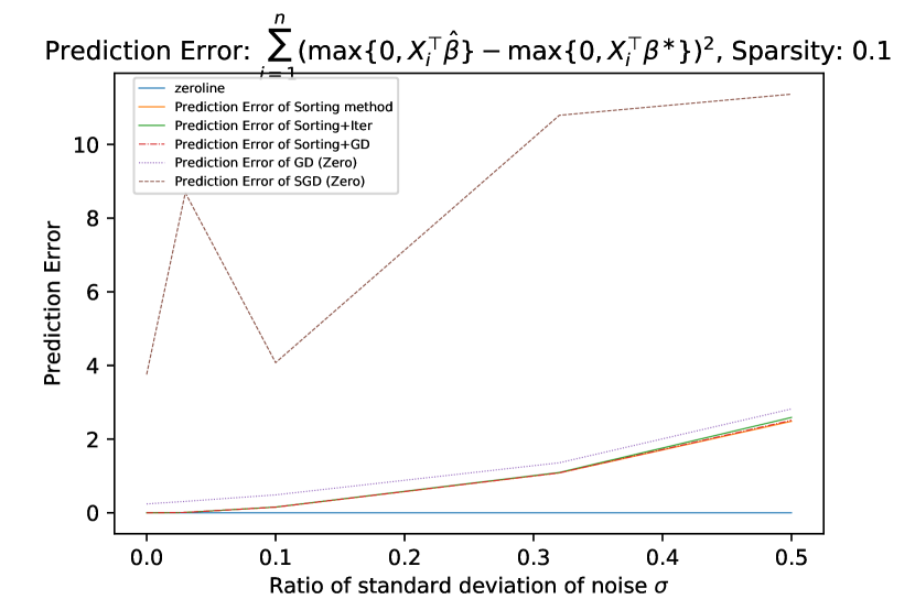
FigureΒ [5, 6] are the continued numerical results that presented in sectionΒ 3.5.

Refer to caption
(a) Prediction Error
Refer to caption
(b) Objective Value
Refer to caption
(c) Recovery Error
Refer to caption
(d) Generalization Error
Refer to caption
(e) Prediction Error
Refer to caption
(f) Objective Value
Refer to caption
(g) Recovery Error
Refer to caption
(h) Generalization Error
Refer to caption
(i) Prediction Error
Refer to caption
(j) Objective Value
Refer to caption
(k) Recovery Error
Refer to caption
(l) Generalization Error
Refer to caption
(m) Prediction Error
Refer to caption
(n) Objective Value
Refer to caption
(o) Recovery Error
Refer to caption
(p) Generalization Error
Refer to caption
(q) Prediction Error
Refer to caption
(r) Objective Value
Refer to caption
(s) Recovery Error
Refer to caption
(t) Generalization Error
Figure 5: Numerical Results of sample size (p,n)=(10,200)𝑝𝑛10200(p,n)=(10,200) and Ξ²βˆ—βˆΌN​(0.5β‹…πŸp,10β‹…Ip)similar-tosuperscriptπ›½βˆ—π‘β‹…0.5subscript1𝑝⋅10subscript𝐼𝑝\beta^{\ast}\sim N(0.5\cdot\mathbf{1}_{p},10\cdot I_{p}) with sparsity {0.1,0.25,0.5,0.75,0.9}0.10.250.50.750.9\{0.1,0.25,0.5,0.75,0.9\}
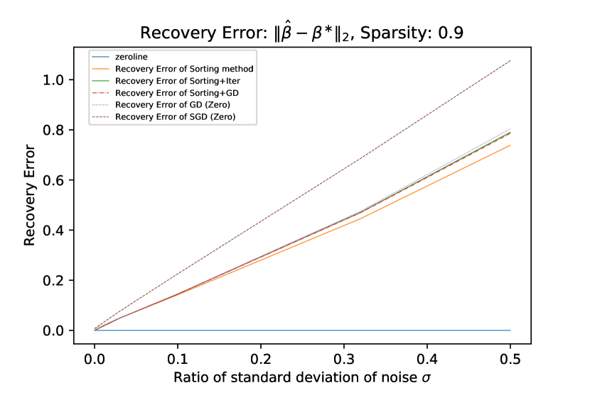
Refer to caption
(a) Prediction Error
Refer to caption
(b) Objective Value
Refer to caption
(c) Recovery Error
Refer to caption
(d) Generalization Error
Refer to caption
(e) Prediction Error
Refer to caption
(f) Objective Value
Refer to caption
(g) Recovery Error
Refer to caption
(h) Generalization Error
Refer to caption
(i) Prediction Error
Refer to caption
(j) Objective Value
Refer to caption
(k) Recovery Error
Refer to caption
(l) Generalization Error
Refer to caption
(m) Prediction Error
Refer to caption
(n) Objective Value
Refer to caption
(o) Recovery Error
Refer to caption
(p) Generalization Error
Refer to caption
(q) Prediction Error
Refer to caption
(r) Objective Value
Refer to caption
(s) Recovery Error
Refer to caption
(t) Generalization Error
Figure 6: Numerical Results of sample size (p,n)=(20,400)𝑝𝑛20400(p,n)=(20,400) and Ξ²βˆ—βˆΌN​(0.5β‹…πŸp,20β‹…Ip)similar-tosuperscriptπ›½βˆ—π‘β‹…0.5subscript1𝑝⋅20subscript𝐼𝑝\beta^{\ast}\sim N(0.5\cdot\mathbf{1}_{p},20\cdot I_{p}) with sparsity {0.1,0.25,0.5,0.75,0.9}0.10.250.50.750.9\{0.1,0.25,0.5,0.75,0.9\}

Appendix F Appendix: Realizable Cases

Note that in realizable cases, since the observation samples {Xi}i=1nsuperscriptsubscriptsubscript𝑋𝑖𝑖1𝑛\{X_{i}\}_{i=1}^{n} are constructed to guarantee the full column rank, i.e., the global optimal solution is unique, then finding a solution with 0 prediction error is equivalent to achieving 0 recovery error. In FigureΒ [6(c), 3(c), 3(g)], the averages of the recovery errors of realizable cases are not zero, however their corresponding prediction errors are very small, this may happen when the methods cannot find out the global optimal solutions. The details of realizable cases are presented in TableΒ [1, 2, 3, 4, 5, 6, 7, 8, 9, 10, 11, 12, 13, 14, 15].

Table 1: Realizable Case p=10,n=200,sparsity=0.1formulae-sequence𝑝10formulae-sequence𝑛200sparsity0.1p=10,n=200,\text{sparsity}=0.1 with Ξ²βˆ—βˆΌN​(0.5β‹…πŸp,10β‹…Ip)similar-tosuperscriptπ›½βˆ—π‘β‹…0.5subscript1𝑝⋅10subscript𝐼𝑝\beta^{\ast}\sim N(0.5\cdot\mathbf{1}_{p},10\cdot I_{p})
Settings Sorting Sorting + Iter Sorting + GD GD SGD
Prediction Recovery Prediction Recovery Prediction Recovery Prediction Recovery Prediction Recovery
(10, 200, 0.0; 1) 0.0 0.0 0.0 0.0 0.0 0.0 0.373 0.265 1.803 0.601
(10, 200, 0.0; 2) 0.0 0.0 0.0 0.0 0.0 0.0 0.191 0.17 0.5 0.265
(10, 200, 0.0; 3) 0.0 0.0 0.0 0.0 0.0 0.0 0.284 0.24 7.214 1.025
(10, 200, 0.0; 4) 0.0 0.0 0.0 0.0 0.0 0.0 0.152 0.138 0.433 0.23
(10, 200, 0.0; 5) 0.0 0.0 0.0 0.0 0.0 0.0 0.335 0.261 1.398 0.467
(10, 200, 0.0; 6) 0.0 0.0 0.0 0.0 0.0 0.0 0.135 0.127 0.226 0.167
(10, 200, 0.0; 7) 0.0 0.0 0.0 0.0 0.0 0.0 0.165 0.149 0.461 0.226
(10, 200, 0.0; 8) 0.0 0.0 0.0 0.0 0.0 0.0 0.145 0.141 0.334 0.2
(10, 200, 0.0; 9) 0.0 0.0 0.0 0.0 0.0 0.0 0.196 0.161 0.745 0.299
(10, 200, 0.0; 10) 0.0 0.0 0.0 0.0 0.0 0.0 0.426 0.294 39.097 2.593
(10, 200, 0.0; 11) 0.0 0.0 0.0 0.0 0.0 0.0 0.306 0.24 0.588 0.314
(10, 200, 0.0; 12) 0.0 0.0 0.0 0.0 0.0 0.0 0.339 0.281 4.137 0.832
(10, 200, 0.0; 13) 0.0 0.0 0.0 0.0 0.0 0.0 0.189 0.165 0.191 0.168
(10, 200, 0.0; 14) 0.0 0.0 0.0 0.0 0.0 0.0 0.386 0.25 0.619 0.297
(10, 200, 0.0; 15) 0.0 0.0 0.0 0.0 0.0 0.0 0.192 0.16 0.664 0.291
(10, 200, 0.0; 16) 0.0 0.0 0.0 0.0 0.0 0.0 0.291 0.218 1.646 0.501
(10, 200, 0.0; 17) 0.0 0.0 0.0 0.0 0.0 0.0 0.205 0.186 0.66 0.312
(10, 200, 0.0; 18) 0.0 0.0 0.0 0.0 0.0 0.0 0.18 0.161 1.234 0.421
(10, 200, 0.0; 19) 0.0 0.0 0.0 0.0 0.0 0.0 0.219 0.184 0.715 0.333
(10, 200, 0.0; 20) 0.0 0.0 0.0 0.0 0.0 0.0 0.142 0.136 12.466 1.2
Table 2: Realizable Case p=10,n=200,sparsity=0.25formulae-sequence𝑝10formulae-sequence𝑛200sparsity0.25p=10,n=200,\text{sparsity}=0.25 with Ξ²βˆ—βˆΌN​(0.5β‹…πŸp,10β‹…Ip)similar-tosuperscriptπ›½βˆ—π‘β‹…0.5subscript1𝑝⋅10subscript𝐼𝑝\beta^{\ast}\sim N(0.5\cdot\mathbf{1}_{p},10\cdot I_{p})
Settings Sorting Sorting + Iter Sorting + GD GD SGD
Prediction Recovery Prediction Recovery Prediction Recovery Prediction Recovery Prediction Recovery
(10, 200, 0.0; 1) 0.0 0.0 0.0 0.0 0.0 0.0 0.049 0.058 0.107 0.084
(10, 200, 0.0; 2) 0.0 0.0 0.0 0.0 0.0 0.0 0.045 0.054 0.088 0.073
(10, 200, 0.0; 3) 0.0 0.0 0.0 0.0 0.0 0.0 0.09 0.088 0.147 0.111
(10, 200, 0.0; 4) 0.0 0.0 0.0 0.0 0.0 0.0 0.025 0.037 0.068 0.065
(10, 200, 0.0; 5) 0.0 0.0 0.0 0.0 0.0 0.0 0.06 0.066 0.929 0.247
(10, 200, 0.0; 6) 0.0 0.0 0.0 0.0 0.0 0.0 0.046 0.058 0.098 0.087
(10, 200, 0.0; 7) 0.0 0.0 0.0 0.0 0.0 0.0 0.044 0.055 0.065 0.06
(10, 200, 0.0; 8) 0.0 0.0 0.0 0.0 0.0 0.0 0.062 0.07 0.11 0.085
(10, 200, 0.0; 9) 0.0 0.0 0.0 0.0 0.0 0.0 0.05 0.059 0.197 0.111
(10, 200, 0.0; 10) 0.0 0.0 0.0 0.0 0.0 0.0 0.083 0.084 0.061 0.069
(10, 200, 0.0; 11) 0.0 0.0 0.0 0.0 0.0 0.0 0.08 0.087 0.125 0.099
(10, 200, 0.0; 12) 0.0 0.0 0.0 0.0 0.0 0.0 0.056 0.064 0.063 0.067
(10, 200, 0.0; 13) 0.0 0.0 0.0 0.0 0.0 0.0 0.054 0.065 0.083 0.072
(10, 200, 0.0; 14) 0.0 0.0 0.0 0.0 0.0 0.0 0.042 0.053 0.285 0.115
(10, 200, 0.0; 15) 0.0 0.0 0.0 0.0 0.0 0.0 0.032 0.039 0.032 0.037
(10, 200, 0.0; 16) 0.0 0.0 0.0 0.0 0.0 0.0 0.073 0.081 0.083 0.072
(10, 200, 0.0; 17) 0.0 0.0 0.0 0.0 0.0 0.0 0.05 0.057 0.071 0.073
(10, 200, 0.0; 18) 0.0 0.0 0.0 0.0 0.0 0.0 0.035 0.044 0.099 0.081
(10, 200, 0.0; 19) 0.0 0.0 0.0 0.0 0.0 0.0 0.038 0.048 0.107 0.077
(10, 200, 0.0; 20) 0.0 0.0 0.0 0.0 0.0 0.0 0.071 0.076 0.207 0.124
Table 3: Realizable Case p=10,n=200,sparsity=0.5formulae-sequence𝑝10formulae-sequence𝑛200sparsity0.5p=10,n=200,\text{sparsity}=0.5 with Ξ²βˆ—βˆΌN​(0.5β‹…πŸp,10β‹…Ip)similar-tosuperscriptπ›½βˆ—π‘β‹…0.5subscript1𝑝⋅10subscript𝐼𝑝\beta^{\ast}\sim N(0.5\cdot\mathbf{1}_{p},10\cdot I_{p})
Settings Sorting Sorting + Iter Sorting + GD GD SGD
Prediction Recovery Prediction Recovery Prediction Recovery Prediction Recovery Prediction Recovery
(10, 200, 0.0; 1) 0.0 0.0 0.0 0.0 0.0 0.0 0.015 0.022 0.043 0.031
(10, 200, 0.0; 2) 0.0 0.0 0.0 0.0 0.0 0.0 0.01 0.017 0.013 0.02
(10, 200, 0.0; 3) 0.0 0.0 0.0 0.0 0.0 0.0 0.016 0.025 0.03 0.029
(10, 200, 0.0; 4) 0.0 0.0 0.0 0.0 0.0 0.0 0.009 0.017 0.025 0.026
(10, 200, 0.0; 5) 0.0 0.0 0.0 0.0 0.0 0.0 0.017 0.024 0.019 0.024
(10, 200, 0.0; 6) 0.0 0.0 0.0 0.0 0.0 0.0 0.015 0.022 0.017 0.02
(10, 200, 0.0; 7) 0.0 0.0 0.0 0.0 0.0 0.0 0.014 0.023 0.075 0.046
(10, 200, 0.0; 8) 0.0 0.0 0.0 0.0 0.0 0.0 0.02 0.028 0.016 0.024
(10, 200, 0.0; 9) 0.0 0.0 0.0 0.0 0.0 0.0 0.025 0.035 0.048 0.044
(10, 200, 0.0; 10) 0.0 0.0 0.0 0.0 0.0 0.0 0.015 0.024 0.017 0.026
(10, 200, 0.0; 11) 0.0 0.0 0.0 0.0 0.0 0.0 0.015 0.024 0.002 0.006
(10, 200, 0.0; 12) 0.0 0.0 0.0 0.0 0.0 0.0 0.008 0.016 0.007 0.013
(10, 200, 0.0; 13) 0.0 0.0 0.0 0.0 0.0 0.0 0.015 0.024 0.018 0.022
(10, 200, 0.0; 14) 0.0 0.0 0.0 0.0 0.0 0.0 0.008 0.015 0.016 0.018
(10, 200, 0.0; 15) 0.0 0.0 0.0 0.0 0.0 0.0 0.014 0.023 0.009 0.015
(10, 200, 0.0; 16) 0.0 0.0 0.0 0.0 0.0 0.0 0.007 0.014 0.024 0.036
(10, 200, 0.0; 17) 0.0 0.0 0.0 0.0 0.0 0.0 0.025 0.034 0.008 0.018
(10, 200, 0.0; 18) 0.0 0.0 0.0 0.0 0.0 0.0 0.011 0.02 0.026 0.027
(10, 200, 0.0; 19) 0.0 0.0 0.0 0.0 0.0 0.0 0.011 0.019 0.007 0.015
(10, 200, 0.0; 20) 0.0 0.0 0.0 0.0 0.0 0.0 0.016 0.025 0.51 0.12
Table 4: Realizable Case p=10,n=200,sparsity=0.75formulae-sequence𝑝10formulae-sequence𝑛200sparsity0.75p=10,n=200,\text{sparsity}=0.75 with Ξ²βˆ—βˆΌN​(0.5β‹…πŸp,10β‹…Ip)similar-tosuperscriptπ›½βˆ—π‘β‹…0.5subscript1𝑝⋅10subscript𝐼𝑝\beta^{\ast}\sim N(0.5\cdot\mathbf{1}_{p},10\cdot I_{p})
Settings Sorting Sorting + Iter Sorting + GD GD SGD
Prediction Recovery Prediction Recovery Prediction Recovery Prediction Recovery Prediction Recovery
(10, 200, 0.0; 1) 0.0 0.0 0.0 0.0 0.0 0.0 0.002 0.006 0.006 0.009
(10, 200, 0.0; 2) 0.0 0.0 0.0 0.0 0.0 0.0 0.008 0.016 0.009 0.012
(10, 200, 0.0; 3) 0.0 0.0 0.0 0.0 0.0 0.0 0.005 0.01 0.01 0.013
(10, 200, 0.0; 4) 0.0 0.0 0.0 0.0 0.0 0.0 0.004 0.009 0.005 0.009
(10, 200, 0.0; 5) 0.0 0.0 0.0 0.0 0.0 0.0 0.006 0.012 0.019 0.017
(10, 200, 0.0; 6) 0.0 0.0 0.0 0.0 0.0 0.0 0.004 0.009 0.013 0.015
(10, 200, 0.0; 7) 0.0 0.0 0.0 0.0 0.0 0.0 0.005 0.011 0.031 0.019
(10, 200, 0.0; 8) 0.0 0.0 0.0 0.0 0.0 0.0 0.001 0.005 0.006 0.009
(10, 200, 0.0; 9) 0.0 0.0 0.0 0.0 0.0 0.0 0.005 0.01 0.005 0.008
(10, 200, 0.0; 10) 0.0 0.0 0.0 0.0 0.0 0.0 0.007 0.012 0.008 0.012
(10, 200, 0.0; 11) 0.0 0.0 0.0 0.0 0.0 0.0 0.005 0.011 0.009 0.012
(10, 200, 0.0; 12) 0.0 0.0 0.0 0.0 0.0 0.0 0.001 0.005 0.003 0.007
(10, 200, 0.0; 13) 0.0 0.0 0.0 0.0 0.0 0.0 0.007 0.014 0.001 0.004
(10, 200, 0.0; 14) 0.0 0.0 0.0 0.0 0.0 0.0 0.003 0.007 0.007 0.009
(10, 200, 0.0; 15) 0.0 0.0 0.0 0.0 0.0 0.0 0.003 0.008 0.007 0.01
(10, 200, 0.0; 16) 0.0 0.0 0.0 0.0 0.0 0.0 0.004 0.009 0.012 0.012
(10, 200, 0.0; 17) 0.0 0.0 0.0 0.0 0.0 0.0 0.008 0.014 0.85 0.101
(10, 200, 0.0; 18) 0.0 0.0 0.0 0.0 0.0 0.0 0.006 0.013 0.017 0.019
(10, 200, 0.0; 19) 0.0 0.0 0.0 0.0 0.0 0.0 0.003 0.008 0.006 0.009
(10, 200, 0.0; 20) 0.0 0.0 0.0 0.0 0.0 0.0 0.01 0.016 0.014 0.013
Table 5: Realizable Case p=10,n=200,sparsity=0.9formulae-sequence𝑝10formulae-sequence𝑛200sparsity0.9p=10,n=200,\text{sparsity}=0.9 with Ξ²βˆ—βˆΌN​(0.5β‹…πŸp,10β‹…Ip)similar-tosuperscriptπ›½βˆ—π‘β‹…0.5subscript1𝑝⋅10subscript𝐼𝑝\beta^{\ast}\sim N(0.5\cdot\mathbf{1}_{p},10\cdot I_{p})
Settings Sorting Sorting + Iter Sorting + GD GD SGD
Prediction Recovery Prediction Recovery Prediction Recovery Prediction Recovery Prediction Recovery
(10, 200, 0.0; 1) 0.0 0.0 0.0 0.0 0.0 0.0 0.006 0.011 0.005 0.01
(10, 200, 0.0; 2) 0.0 0.0 0.0 0.0 0.0 0.0 0.009 0.016 0.028 0.02
(10, 200, 0.0; 3) 0.0 0.0 0.0 0.0 0.0 0.0 0.005 0.011 0.044 0.022
(10, 200, 0.0; 4) 0.0 0.0 0.0 0.0 0.0 0.0 0.001 0.002 0.012 0.013
(10, 200, 0.0; 5) 0.0 0.0 0.0 0.0 0.0 0.0 0.004 0.009 0.002 0.005
(10, 200, 0.0; 6) 0.0 0.0 0.0 0.0 0.0 0.0 0.0 0.001 0.007 0.008
(10, 200, 0.0; 7) 0.0 0.0 0.0 0.0 0.0 0.0 0.005 0.011 0.019 0.019
(10, 200, 0.0; 8) 0.0 0.0 0.0 0.0 0.0 0.0 0.004 0.009 0.011 0.013
(10, 200, 0.0; 9) 0.0 0.0 0.0 0.0 0.0 0.0 0.001 0.005 0.006 0.008
(10, 200, 0.0; 10) 0.0 0.0 0.0 0.0 0.0 0.0 0.002 0.006 0.007 0.009
(10, 200, 0.0; 11) 0.0 0.0 0.0 0.0 0.0 0.0 0.002 0.006 0.004 0.007
(10, 200, 0.0; 12) 0.0 0.0 0.0 0.0 0.0 0.0 0.001 0.005 0.01 0.011
(10, 200, 0.0; 13) 0.0 0.0 0.0 0.0 0.0 0.0 0.005 0.011 0.026 0.019
(10, 200, 0.0; 14) 0.0 0.0 0.0 0.0 0.0 0.0 0.001 0.005 0.004 0.006
(10, 200, 0.0; 15) 0.0 0.0 0.0 0.0 0.0 0.0 0.002 0.006 0.01 0.011
(10, 200, 0.0; 16) 0.0 0.0 0.0 0.0 0.0 0.0 0.004 0.01 0.02 0.013
(10, 200, 0.0; 17) 0.0 0.0 0.0 0.0 0.0 0.0 0.0 0.001 0.118 0.031
(10, 200, 0.0; 18) 0.0 0.0 0.0 0.0 0.0 0.0 0.003 0.009 0.034 0.018
(10, 200, 0.0; 19) 0.0 0.0 0.0 0.0 0.0 0.0 0.002 0.006 0.023 0.016
(10, 200, 0.0; 20) 0.0 0.0 0.0 0.0 0.0 0.0 0.006 0.011 0.014 0.012
Table 6: Realizable Case p=20,n=400,sparsity=0.1formulae-sequence𝑝20formulae-sequence𝑛400sparsity0.1p=20,n=400,\text{sparsity}=0.1 with Ξ²βˆ—βˆΌN​(0.5β‹…πŸp,10β‹…Ip)similar-tosuperscriptπ›½βˆ—π‘β‹…0.5subscript1𝑝⋅10subscript𝐼𝑝\beta^{\ast}\sim N(0.5\cdot\mathbf{1}_{p},10\cdot I_{p})
Settings Sorting Sorting + Iter Sorting + GD GD SGD
Prediction Recovery Prediction Recovery Prediction Recovery Prediction Recovery Prediction Recovery
(20, 400, 0.0; 1) 0.0 0.0 0.0 0.0 0.0 0.0 0.256 0.142 0.391 0.178
(20, 400, 0.0; 2) 0.0 0.0 0.0 0.0 0.0 0.0 0.436 0.214 0.79 0.281
(20, 400, 0.0; 3) 0.0 0.0 0.0 0.0 0.0 0.0 0.295 0.157 0.401 0.18
(20, 400, 0.0; 4) 0.0 0.0 0.0 0.0 0.0 0.0 0.332 0.171 0.325 0.158
(20, 400, 0.0; 5) 0.0 0.0 0.0 0.0 0.0 0.0 0.288 0.157 0.598 0.22
(20, 400, 0.0; 6) 0.0 0.0 0.0 0.0 0.0 0.0 0.43 0.196 0.633 0.232
(20, 400, 0.0; 7) 0.0 0.0 0.0 0.0 0.0 0.0 0.257 0.146 0.431 0.19
(20, 400, 0.0; 8) 0.0 0.0 0.0 0.0 0.0 0.0 0.48 0.226 0.667 0.259
(20, 400, 0.0; 9) 0.0 0.0 0.0 0.0 0.0 0.0 0.457 0.204 1.063 0.31
(20, 400, 0.0; 10) 0.0 0.0 0.0 0.0 0.0 0.0 0.226 0.135 0.404 0.177
(20, 400, 0.0; 11) 0.0 0.0 0.0 0.0 0.0 0.0 0.301 0.16 0.481 0.189
(20, 400, 0.0; 12) 0.0 0.0 0.0 0.0 0.0 0.0 0.383 0.183 1.135 0.31
(20, 400, 0.0; 13) 0.0 0.0 0.0 0.0 0.0 0.0 0.33 0.162 1.007 0.278
(20, 400, 0.0; 14) 0.0 0.0 0.0 0.0 0.0 0.0 0.336 0.173 0.478 0.201
(20, 400, 0.0; 15) 0.0 0.0 0.0 0.0 0.0 0.0 0.305 0.163 0.5 0.199
(20, 400, 0.0; 16) 0.0 0.0 0.0 0.0 0.0 0.0 0.272 0.152 0.5 0.198
(20, 400, 0.0; 17) 0.0 0.0 0.0 0.0 0.0 0.0 0.313 0.169 0.274 0.146
(20, 400, 0.0; 18) 0.0 0.0 0.0 0.0 0.0 0.0 0.288 0.154 0.338 0.169
(20, 400, 0.0; 19) 0.0 0.0 0.0 0.0 0.0 0.0 0.548 0.255 1.103 0.355
(20, 400, 0.0; 20) 0.0 0.0 0.0 0.0 0.0 0.0 0.313 0.16 0.383 0.172
Table 7: Realizable Case p=20,n=400,sparsity=0.25formulae-sequence𝑝20formulae-sequence𝑛400sparsity0.25p=20,n=400,\text{sparsity}=0.25 with Ξ²βˆ—βˆΌN​(0.5β‹…πŸp,10β‹…Ip)similar-tosuperscriptπ›½βˆ—π‘β‹…0.5subscript1𝑝⋅10subscript𝐼𝑝\beta^{\ast}\sim N(0.5\cdot\mathbf{1}_{p},10\cdot I_{p})
Settings Sorting Sorting + Iter Sorting + GD GD SGD
Prediction Recovery Prediction Recovery Prediction Recovery Prediction Recovery Prediction Recovery
(20, 400, 0.0; 1) 0.0 0.0 0.0 0.0 0.0 0.0 0.064 0.05 0.061 0.046
(20, 400, 0.0; 2) 0.0 0.0 0.0 0.0 0.0 0.0 0.051 0.04 0.039 0.035
(20, 400, 0.0; 3) 0.0 0.0 0.0 0.0 0.0 0.0 0.069 0.05 0.119 0.063
(20, 400, 0.0; 4) 0.0 0.0 0.0 0.0 0.0 0.0 0.061 0.045 0.078 0.051
(20, 400, 0.0; 5) 0.0 0.0 0.0 0.0 0.0 0.0 0.059 0.046 0.065 0.046
(20, 400, 0.0; 6) 0.0 0.0 0.0 0.0 0.0 0.0 0.061 0.046 0.248 0.089
(20, 400, 0.0; 7) 0.0 0.0 0.0 0.0 0.0 0.0 0.11 0.074 0.245 0.109
(20, 400, 0.0; 8) 0.0 0.0 0.0 0.0 0.0 0.0 0.054 0.043 0.12 0.06
(20, 400, 0.0; 9) 0.0 0.0 0.0 0.0 0.0 0.0 0.079 0.055 0.087 0.057
(20, 400, 0.0; 10) 0.0 0.0 0.0 0.0 0.0 0.0 0.065 0.052 0.078 0.054
(20, 400, 0.0; 11) 0.0 0.0 0.0 0.0 0.0 0.0 0.093 0.067 0.111 0.066
(20, 400, 0.0; 12) 0.0 0.0 0.0 0.0 0.0 0.0 0.082 0.058 0.118 0.073
(20, 400, 0.0; 13) 0.0 0.0 0.0 0.0 0.0 0.0 0.067 0.05 0.085 0.057
(20, 400, 0.0; 14) 0.0 0.0 0.0 0.0 0.0 0.0 0.05 0.042 0.06 0.042
(20, 400, 0.0; 15) 0.0 0.0 0.0 0.0 0.0 0.0 0.065 0.05 0.12 0.067
(20, 400, 0.0; 16) 0.0 0.0 0.0 0.0 0.0 0.0 0.093 0.065 0.117 0.07
(20, 400, 0.0; 17) 0.0 0.0 0.0 0.0 0.0 0.0 0.097 0.065 0.133 0.072
(20, 400, 0.0; 18) 0.0 0.0 0.0 0.0 0.0 0.0 0.067 0.049 0.09 0.057
(20, 400, 0.0; 19) 0.0 0.0 0.0 0.0 0.0 0.0 0.073 0.054 0.084 0.057
(20, 400, 0.0; 20) 0.0 0.0 0.0 0.0 0.0 0.0 0.049 0.039 0.108 0.057
Table 8: Realizable Case p=20,n=400,sparsity=0.5formulae-sequence𝑝20formulae-sequence𝑛400sparsity0.5p=20,n=400,\text{sparsity}=0.5 with Ξ²βˆ—βˆΌN​(0.5β‹…πŸp,10β‹…Ip)similar-tosuperscriptπ›½βˆ—π‘β‹…0.5subscript1𝑝⋅10subscript𝐼𝑝\beta^{\ast}\sim N(0.5\cdot\mathbf{1}_{p},10\cdot I_{p})
Settings Sorting Sorting + Iter Sorting + GD GD SGD
Prediction Recovery Prediction Recovery Prediction Recovery Prediction Recovery Prediction Recovery
(20, 400, 0.0; 1) 0.0 0.0 0.0 0.0 0.0 0.0 0.028 0.026 0.021 0.02
(20, 400, 0.0; 2) 0.0 0.0 0.0 0.0 0.0 0.0 0.018 0.018 0.026 0.021
(20, 400, 0.0; 3) 0.0 0.0 0.0 0.0 0.0 0.0 0.015 0.016 0.023 0.018
(20, 400, 0.0; 4) 0.0 0.0 0.0 0.0 0.0 0.0 0.018 0.019 0.034 0.024
(20, 400, 0.0; 5) 0.0 0.0 0.0 0.0 0.0 0.0 0.01 0.013 0.014 0.014
(20, 400, 0.0; 6) 0.0 0.0 0.0 0.0 0.0 0.0 0.02 0.019 0.017 0.016
(20, 400, 0.0; 7) 0.0 0.0 0.0 0.0 0.0 0.0 0.01 0.013 0.011 0.012
(20, 400, 0.0; 8) 0.0 0.0 0.0 0.0 0.0 0.0 0.022 0.021 0.022 0.018
(20, 400, 0.0; 9) 0.0 0.0 0.0 0.0 0.0 0.0 0.016 0.018 0.005 0.009
(20, 400, 0.0; 10) 0.0 0.0 0.0 0.0 0.0 0.0 0.016 0.017 0.029 0.02
(20, 400, 0.0; 11) 0.0 0.0 0.0 0.0 0.0 0.0 0.022 0.021 0.043 0.025
(20, 400, 0.0; 12) 0.0 0.0 0.0 0.0 0.0 0.0 0.019 0.019 0.017 0.017
(20, 400, 0.0; 13) 0.0 0.0 0.0 0.0 0.0 0.0 0.017 0.017 0.014 0.015
(20, 400, 0.0; 14) 0.0 0.0 0.0 0.0 0.0 0.0 0.019 0.02 0.034 0.025
(20, 400, 0.0; 15) 0.0 0.0 0.0 0.0 0.0 0.0 0.015 0.016 0.015 0.014
(20, 400, 0.0; 16) 0.0 0.0 0.0 0.0 0.0 0.0 0.017 0.017 0.011 0.012
(20, 400, 0.0; 17) 0.0 0.0 0.0 0.0 0.0 0.0 0.024 0.022 0.065 0.031
(20, 400, 0.0; 18) 0.0 0.0 0.0 0.0 0.0 0.0 0.017 0.017 0.011 0.014
(20, 400, 0.0; 19) 0.0 0.0 0.0 0.0 0.0 0.0 0.017 0.018 0.022 0.018
(20, 400, 0.0; 20) 0.0 0.0 0.0 0.0 0.0 0.0 0.019 0.019 0.02 0.016
Table 9: Realizable Case p=20,n=400,sparsity=0.75formulae-sequence𝑝20formulae-sequence𝑛400sparsity0.75p=20,n=400,\text{sparsity}=0.75 with Ξ²βˆ—βˆΌN​(0.5β‹…πŸp,10β‹…Ip)similar-tosuperscriptπ›½βˆ—π‘β‹…0.5subscript1𝑝⋅10subscript𝐼𝑝\beta^{\ast}\sim N(0.5\cdot\mathbf{1}_{p},10\cdot I_{p})
Settings Sorting Sorting + Iter Sorting + GD GD SGD
Prediction Recovery Prediction Recovery Prediction Recovery Prediction Recovery Prediction Recovery
(20, 400, 0.0; 1) 0.0 0.0 0.0 0.0 0.0 0.0 0.01 0.012 0.02 0.013
(20, 400, 0.0; 2) 0.0 0.0 0.0 0.0 0.0 0.0 0.006 0.008 0.006 0.006
(20, 400, 0.0; 3) 0.0 0.0 0.0 0.0 0.0 0.0 0.003 0.005 0.005 0.006
(20, 400, 0.0; 4) 0.0 0.0 0.0 0.0 0.0 0.0 0.009 0.011 0.027 0.015
(20, 400, 0.0; 5) 0.0 0.0 0.0 0.0 0.0 0.0 0.009 0.011 0.008 0.009
(20, 400, 0.0; 6) 0.0 0.0 0.0 0.0 0.0 0.0 0.009 0.012 0.016 0.013
(20, 400, 0.0; 7) 0.0 0.0 0.0 0.0 0.0 0.0 0.005 0.008 0.009 0.008
(20, 400, 0.0; 8) 0.0 0.0 0.0 0.0 0.0 0.0 0.003 0.005 0.013 0.01
(20, 400, 0.0; 9) 0.0 0.0 0.0 0.0 0.0 0.0 0.007 0.01 0.01 0.009
(20, 400, 0.0; 10) 0.0 0.0 0.0 0.0 0.0 0.0 0.007 0.009 0.007 0.007
(20, 400, 0.0; 11) 0.0 0.0 0.0 0.0 0.0 0.0 0.008 0.01 0.014 0.01
(20, 400, 0.0; 12) 0.0 0.0 0.0 0.0 0.0 0.0 0.011 0.012 0.01 0.009
(20, 400, 0.0; 13) 0.0 0.0 0.0 0.0 0.0 0.0 0.005 0.008 0.007 0.008
(20, 400, 0.0; 14) 0.0 0.0 0.0 0.0 0.0 0.0 0.007 0.009 0.012 0.009
(20, 400, 0.0; 15) 0.0 0.0 0.0 0.0 0.0 0.0 0.005 0.008 0.003 0.004
(20, 400, 0.0; 16) 0.0 0.0 0.0 0.0 0.0 0.0 0.005 0.007 0.011 0.009
(20, 400, 0.0; 17) 0.0 0.0 0.0 0.0 0.0 0.0 0.006 0.009 0.011 0.01
(20, 400, 0.0; 18) 0.0 0.0 0.0 0.0 0.0 0.0 0.005 0.008 0.011 0.009
(20, 400, 0.0; 19) 0.0 0.0 0.0 0.0 0.0 0.0 0.01 0.012 0.01 0.01
(20, 400, 0.0; 20) 0.0 0.0 0.0 0.0 0.0 0.0 0.012 0.014 0.032 0.018
Table 10: Realizable Case p=20,n=400,sparsity=0.9formulae-sequence𝑝20formulae-sequence𝑛400sparsity0.9p=20,n=400,\text{sparsity}=0.9 with Ξ²βˆ—βˆΌN​(0.5β‹…πŸp,10β‹…Ip)similar-tosuperscriptπ›½βˆ—π‘β‹…0.5subscript1𝑝⋅10subscript𝐼𝑝\beta^{\ast}\sim N(0.5\cdot\mathbf{1}_{p},10\cdot I_{p})
Settings Sorting Sorting + Iter Sorting + GD GD SGD
Prediction Recovery Prediction Recovery Prediction Recovery Prediction Recovery Prediction Recovery
(20, 400, 0.0; 1) 0.0 0.0 0.0 0.0 0.0 0.0 0.004 0.007 0.005 0.006
(20, 400, 0.0; 2) 0.0 0.0 0.0 0.0 0.0 0.0 0.004 0.006 0.009 0.008
(20, 400, 0.0; 3) 0.0 0.0 0.0 0.0 0.0 0.0 0.005 0.007 0.006 0.005
(20, 400, 0.0; 4) 0.0 0.0 0.0 0.0 0.0 0.0 0.002 0.004 0.02 0.012
(20, 400, 0.0; 5) 0.0 0.0 0.0 0.0 0.0 0.0 0.003 0.005 0.006 0.006
(20, 400, 0.0; 6) 0.0 0.0 0.0 0.0 0.0 0.0 0.003 0.005 0.003 0.004
(20, 400, 0.0; 7) 0.0 0.0 0.0 0.0 0.0 0.0 0.005 0.008 0.01 0.009
(20, 400, 0.0; 8) 0.0 0.0 0.0 0.0 0.0 0.0 0.006 0.008 0.006 0.006
(20, 400, 0.0; 9) 0.0 0.0 0.0 0.0 0.0 0.0 0.003 0.006 0.012 0.008
(20, 400, 0.0; 10) 0.0 0.0 0.0 0.0 0.0 0.0 0.005 0.008 0.007 0.006
(20, 400, 0.0; 11) 0.0 0.0 0.0 0.0 0.0 0.0 0.004 0.007 0.014 0.009
(20, 400, 0.0; 12) 0.0 0.0 0.0 0.0 0.0 0.0 0.006 0.008 0.009 0.007
(20, 400, 0.0; 13) 0.0 0.0 0.0 0.0 0.0 0.0 0.006 0.008 0.006 0.006
(20, 400, 0.0; 14) 0.0 0.0 0.0 0.0 0.0 0.0 0.007 0.008 0.018 0.011
(20, 400, 0.0; 15) 0.0 0.0 0.0 0.0 0.0 0.0 0.004 0.006 0.007 0.007
(20, 400, 0.0; 16) 0.0 0.0 0.0 0.0 0.0 0.0 0.003 0.005 0.004 0.005
(20, 400, 0.0; 17) 0.0 0.0 0.0 0.0 0.0 0.0 0.006 0.009 0.006 0.006
(20, 400, 0.0; 18) 0.0 0.0 0.0 0.0 0.0 0.0 0.005 0.007 0.004 0.005
(20, 400, 0.0; 19) 0.0 0.0 0.0 0.0 0.0 0.0 0.001 0.003 0.013 0.008
(20, 400, 0.0; 20) 0.0 0.0 0.0 0.0 0.0 0.0 0.005 0.007 0.011 0.008
Table 11: Realizable Case p=50,n=1000,sparsity=0.1formulae-sequence𝑝50formulae-sequence𝑛1000sparsity0.1p=50,n=1000,\text{sparsity}=0.1 with Ξ²βˆ—βˆΌN​(0.5β‹…πŸp,10β‹…Ip)similar-tosuperscriptπ›½βˆ—π‘β‹…0.5subscript1𝑝⋅10subscript𝐼𝑝\beta^{\ast}\sim N(0.5\cdot\mathbf{1}_{p},10\cdot I_{p})
Settings Sorting Sorting + Iter Sorting + GD GD SGD
Prediction Recovery Prediction Recovery Prediction Recovery Prediction Recovery Prediction Recovery
(50, 1000, 0.0; 1) 0.0 0.0 0.0 0.0 0.0 0.0 0.715 0.17 1.104 0.21
(50, 1000, 0.0; 2) 0.0 0.0 0.0 0.0 0.0 0.0 0.601 0.154 0.787 0.175
(50, 1000, 0.0; 3) 0.0 0.0 0.0 0.0 0.0 0.0 0.661 0.167 0.741 0.175
(50, 1000, 0.0; 4) 0.0 0.0 0.0 0.0 0.0 0.0 0.551 0.143 0.631 0.151
(50, 1000, 0.0; 5) 0.0 0.0 0.0 0.0 0.0 0.0 0.528 0.144 0.661 0.16
(50, 1000, 0.0; 6) 0.0 0.0 0.0 0.0 0.0 0.0 0.347 0.105 0.417 0.112
(50, 1000, 0.0; 7) 0.0 0.0 0.0 0.0 0.0 0.0 0.493 0.13 0.586 0.141
(50, 1000, 0.0; 8) 0.0 0.0 0.0 0.0 0.0 0.0 0.526 0.141 0.814 0.176
(50, 1000, 0.0; 9) 0.0 0.0 0.0 0.0 0.0 0.0 0.46 0.128 0.848 0.173
(50, 1000, 0.0; 10) 0.0 0.0 0.0 0.0 0.0 0.0 0.571 0.15 0.703 0.167
(50, 1000, 0.0; 11) 0.0 0.0 0.0 0.0 0.0 0.0 0.641 0.157 0.883 0.183
(50, 1000, 0.0; 12) 0.0 0.0 0.0 0.0 0.0 0.0 0.601 0.157 0.785 0.179
(50, 1000, 0.0; 13) 0.0 0.0 0.0 0.0 0.0 0.0 0.581 0.144 0.871 0.176
(50, 1000, 0.0; 14) 0.0 0.0 0.0 0.0 0.0 0.0 0.469 0.126 0.569 0.139
(50, 1000, 0.0; 15) 0.0 0.0 0.0 0.0 0.0 0.0 0.535 0.14 0.882 0.181
(50, 1000, 0.0; 16) 0.0 0.0 0.0 0.0 0.0 0.0 0.7 0.168 0.85 0.184
(50, 1000, 0.0; 17) 0.0 0.0 0.0 0.0 0.0 0.0 0.613 0.156 0.881 0.182
(50, 1000, 0.0; 18) 0.0 0.0 0.0 0.0 0.0 0.0 0.551 0.142 0.802 0.17
(50, 1000, 0.0; 19) 0.0 0.0 0.0 0.0 0.0 0.0 0.475 0.131 0.589 0.148
(50, 1000, 0.0; 20) 0.0 0.0 0.0 0.0 0.0 0.0 0.566 0.149 0.608 0.154
Table 12: Realizable Case p=50,n=1000,sparsity=0.25formulae-sequence𝑝50formulae-sequence𝑛1000sparsity0.25p=50,n=1000,\text{sparsity}=0.25 with Ξ²βˆ—βˆΌN​(0.5β‹…πŸp,10β‹…Ip)similar-tosuperscriptπ›½βˆ—π‘β‹…0.5subscript1𝑝⋅10subscript𝐼𝑝\beta^{\ast}\sim N(0.5\cdot\mathbf{1}_{p},10\cdot I_{p})
Settings Sorting Sorting + Iter Sorting + GD GD SGD
Prediction Recovery Prediction Recovery Prediction Recovery Prediction Recovery Prediction Recovery
(50, 1000, 0.0; 1) 0.0 0.0 0.0 0.0 0.0 0.0 0.096 0.04 0.128 0.045
(50, 1000, 0.0; 2) 0.0 0.0 0.0 0.0 0.0 0.0 0.073 0.033 0.075 0.031
(50, 1000, 0.0; 3) 0.0 0.0 0.0 0.0 0.0 0.0 0.092 0.038 0.073 0.033
(50, 1000, 0.0; 4) 0.0 0.0 0.0 0.0 0.0 0.0 0.09 0.038 0.071 0.032
(50, 1000, 0.0; 5) 0.0 0.0 0.0 0.0 0.0 0.0 0.095 0.039 0.107 0.04
(50, 1000, 0.0; 6) 0.0 0.0 0.0 0.0 0.0 0.0 0.112 0.044 0.145 0.051
(50, 1000, 0.0; 7) 0.0 0.0 0.0 0.0 0.0 0.0 0.086 0.037 0.078 0.034
(50, 1000, 0.0; 8) 0.0 0.0 0.0 0.0 0.0 0.0 0.091 0.037 0.136 0.045
(50, 1000, 0.0; 9) 0.0 0.0 0.0 0.0 0.0 0.0 0.1 0.041 0.091 0.038
(50, 1000, 0.0; 10) 0.0 0.0 0.0 0.0 0.0 0.0 0.121 0.047 0.104 0.042
(50, 1000, 0.0; 11) 0.0 0.0 0.0 0.0 0.0 0.0 0.078 0.033 0.097 0.037
(50, 1000, 0.0; 12) 0.0 0.0 0.0 0.0 0.0 0.0 0.088 0.038 0.088 0.035
(50, 1000, 0.0; 13) 0.0 0.0 0.0 0.0 0.0 0.0 0.073 0.033 0.073 0.03
(50, 1000, 0.0; 14) 0.0 0.0 0.0 0.0 0.0 0.0 0.088 0.037 0.124 0.042
(50, 1000, 0.0; 15) 0.0 0.0 0.0 0.0 0.0 0.0 0.082 0.036 0.106 0.038
(50, 1000, 0.0; 16) 0.0 0.0 0.0 0.0 0.0 0.0 0.067 0.03 0.144 0.044
(50, 1000, 0.0; 17) 0.0 0.0 0.0 0.0 0.0 0.0 0.101 0.04 0.132 0.045
(50, 1000, 0.0; 18) 0.0 0.0 0.0 0.0 0.0 0.0 0.083 0.035 0.121 0.041
(50, 1000, 0.0; 19) 0.0 0.0 0.0 0.0 0.0 0.0 0.093 0.039 0.107 0.041
(50, 1000, 0.0; 20) 0.0 0.0 0.0 0.0 0.0 0.0 0.1 0.04 0.251 0.062
Table 13: Realizable Case p=50,n=1000,sparsity=0.5formulae-sequence𝑝50formulae-sequence𝑛1000sparsity0.5p=50,n=1000,\text{sparsity}=0.5 with Ξ²βˆ—βˆΌN​(0.5β‹…πŸp,10β‹…Ip)similar-tosuperscriptπ›½βˆ—π‘β‹…0.5subscript1𝑝⋅10subscript𝐼𝑝\beta^{\ast}\sim N(0.5\cdot\mathbf{1}_{p},10\cdot I_{p})
Settings Sorting Sorting + Iter Sorting + GD GD SGD
Prediction Recovery Prediction Recovery Prediction Recovery Prediction Recovery Prediction Recovery
(50, 1000, 0.0; 1) 0.0 0.0 0.0 0.0 0.0 0.0 0.026 0.015 0.037 0.016
(50, 1000, 0.0; 2) 0.0 0.0 0.0 0.0 0.0 0.0 0.026 0.015 0.034 0.016
(50, 1000, 0.0; 3) 0.0 0.0 0.0 0.0 0.0 0.0 0.028 0.016 0.045 0.018
(50, 1000, 0.0; 4) 0.0 0.0 0.0 0.0 0.0 0.0 0.024 0.014 0.021 0.012
(50, 1000, 0.0; 5) 0.0 0.0 0.0 0.0 0.0 0.0 0.02 0.012 0.028 0.014
(50, 1000, 0.0; 6) 0.0 0.0 0.0 0.0 0.0 0.0 0.02 0.012 0.022 0.012
(50, 1000, 0.0; 7) 0.0 0.0 0.0 0.0 0.0 0.0 0.017 0.011 0.024 0.012
(50, 1000, 0.0; 8) 0.0 0.0 0.0 0.0 0.0 0.0 0.022 0.013 0.039 0.016
(50, 1000, 0.0; 9) 0.0 0.0 0.0 0.0 0.0 0.0 0.019 0.011 0.015 0.009
(50, 1000, 0.0; 10) 0.0 0.0 0.0 0.0 0.0 0.0 0.019 0.012 0.034 0.015
(50, 1000, 0.0; 11) 0.0 0.0 0.0 0.0 0.0 0.0 0.018 0.012 0.014 0.009
(50, 1000, 0.0; 12) 0.0 0.0 0.0 0.0 0.0 0.0 0.024 0.014 0.02 0.011
(50, 1000, 0.0; 13) 0.0 0.0 0.0 0.0 0.0 0.0 0.024 0.015 0.039 0.017
(50, 1000, 0.0; 14) 0.0 0.0 0.0 0.0 0.0 0.0 0.037 0.019 0.04 0.017
(50, 1000, 0.0; 15) 0.0 0.0 0.0 0.0 0.0 0.0 0.021 0.013 0.042 0.016
(50, 1000, 0.0; 16) 0.0 0.0 0.0 0.0 0.0 0.0 0.02 0.013 0.053 0.019
(50, 1000, 0.0; 17) 0.0 0.0 0.0 0.0 0.0 0.0 0.019 0.012 0.017 0.011
(50, 1000, 0.0; 18) 0.0 0.0 0.0 0.0 0.0 0.0 0.015 0.01 0.014 0.009
(50, 1000, 0.0; 19) 0.0 0.0 0.0 0.0 0.0 0.0 0.018 0.012 0.034 0.016
(50, 1000, 0.0; 20) 0.0 0.0 0.0 0.0 0.0 0.0 0.019 0.012 0.015 0.01
Table 14: Realizable Case p=50,n=1000,sparsity=0.75formulae-sequence𝑝50formulae-sequence𝑛1000sparsity0.75p=50,n=1000,\text{sparsity}=0.75 with Ξ²βˆ—βˆΌN​(0.5β‹…πŸp,10β‹…Ip)similar-tosuperscriptπ›½βˆ—π‘β‹…0.5subscript1𝑝⋅10subscript𝐼𝑝\beta^{\ast}\sim N(0.5\cdot\mathbf{1}_{p},10\cdot I_{p})
Settings Sorting Sorting + Iter Sorting + GD GD SGD
Prediction Recovery Prediction Recovery Prediction Recovery Prediction Recovery Prediction Recovery
(50, 1000, 0.0; 1) 0.0 0.0 0.0 0.0 0.0 0.0 0.009 0.007 0.009 0.006
(50, 1000, 0.0; 2) 0.0 0.0 0.0 0.0 0.0 0.0 0.011 0.008 0.014 0.007
(50, 1000, 0.0; 3) 0.0 0.0 0.0 0.0 0.0 0.0 0.011 0.008 0.027 0.01
(50, 1000, 0.0; 4) 0.0 0.0 0.0 0.0 0.0 0.0 0.01 0.007 0.01 0.006
(50, 1000, 0.0; 5) 0.0 0.0 0.0 0.0 0.0 0.0 0.008 0.006 0.015 0.007
(50, 1000, 0.0; 6) 0.0 0.0 0.0 0.0 0.0 0.0 0.005 0.005 0.008 0.005
(50, 1000, 0.0; 7) 0.0 0.0 0.0 0.0 0.0 0.0 0.016 0.01 0.006 0.005
(50, 1000, 0.0; 8) 0.0 0.0 0.0 0.0 0.0 0.0 0.007 0.006 0.009 0.006
(50, 1000, 0.0; 9) 0.0 0.0 0.0 0.0 0.0 0.0 0.012 0.008 0.011 0.006
(50, 1000, 0.0; 10) 0.0 0.0 0.0 0.0 0.0 0.0 0.008 0.007 0.022 0.009
(50, 1000, 0.0; 11) 0.0 0.0 0.0 0.0 0.0 0.0 0.007 0.006 0.01 0.006
(50, 1000, 0.0; 12) 0.0 0.0 0.0 0.0 0.0 0.0 0.008 0.006 0.014 0.007
(50, 1000, 0.0; 13) 0.0 0.0 0.0 0.0 0.0 0.0 0.007 0.006 0.008 0.006
(50, 1000, 0.0; 14) 0.0 0.0 0.0 0.0 0.0 0.0 0.006 0.006 0.026 0.011
(50, 1000, 0.0; 15) 0.0 0.0 0.0 0.0 0.0 0.0 0.007 0.006 0.006 0.005
(50, 1000, 0.0; 16) 0.0 0.0 0.0 0.0 0.0 0.0 0.006 0.005 0.011 0.006
(50, 1000, 0.0; 17) 0.0 0.0 0.0 0.0 0.0 0.0 0.006 0.005 0.01 0.006
(50, 1000, 0.0; 18) 0.0 0.0 0.0 0.0 0.0 0.0 0.009 0.007 0.007 0.005
(50, 1000, 0.0; 19) 0.0 0.0 0.0 0.0 0.0 0.0 0.006 0.006 0.011 0.007
(50, 1000, 0.0; 20) 0.0 0.0 0.0 0.0 0.0 0.0 0.011 0.008 0.014 0.007
Table 15: Realizable Case p=50,n=1000,sparsity=0.9formulae-sequence𝑝50formulae-sequence𝑛1000sparsity0.9p=50,n=1000,\text{sparsity}=0.9 with Ξ²βˆ—βˆΌN​(0.5β‹…πŸp,10β‹…Ip)similar-tosuperscriptπ›½βˆ—π‘β‹…0.5subscript1𝑝⋅10subscript𝐼𝑝\beta^{\ast}\sim N(0.5\cdot\mathbf{1}_{p},10\cdot I_{p})
Settings Sorting Sorting + Iter Sorting + GD GD SGD
Prediction Recovery Prediction Recovery Prediction Recovery Prediction Recovery Prediction Recovery
(50, 1000, 0.0; 1) 0.0 0.0 0.0 0.0 0.0 0.0 0.005 0.005 0.006 0.004
(50, 1000, 0.0; 2) 0.0 0.0 0.0 0.0 0.0 0.0 0.006 0.005 0.009 0.005
(50, 1000, 0.0; 3) 0.0 0.0 0.0 0.0 0.0 0.0 0.005 0.005 0.008 0.005
(50, 1000, 0.0; 4) 0.0 0.0 0.0 0.0 0.0 0.0 0.002 0.003 0.03 0.009
(50, 1000, 0.0; 5) 0.0 0.0 0.0 0.0 0.0 0.0 0.004 0.004 0.009 0.005
(50, 1000, 0.0; 6) 0.0 0.0 0.0 0.0 0.0 0.0 0.008 0.006 0.008 0.005
(50, 1000, 0.0; 7) 0.0 0.0 0.0 0.0 0.0 0.0 0.008 0.006 0.01 0.005
(50, 1000, 0.0; 8) 0.0 0.0 0.0 0.0 0.0 0.0 0.005 0.005 0.012 0.005
(50, 1000, 0.0; 9) 0.0 0.0 0.0 0.0 0.0 0.0 0.009 0.007 0.01 0.006
(50, 1000, 0.0; 10) 0.0 0.0 0.0 0.0 0.0 0.0 0.005 0.004 0.01 0.005
(50, 1000, 0.0; 11) 0.0 0.0 0.0 0.0 0.0 0.0 0.008 0.006 0.005 0.004
(50, 1000, 0.0; 12) 0.0 0.0 0.0 0.0 0.0 0.0 0.007 0.006 0.006 0.004
(50, 1000, 0.0; 13) 0.0 0.0 0.0 0.0 0.0 0.0 0.005 0.005 0.007 0.004
(50, 1000, 0.0; 14) 0.0 0.0 0.0 0.0 0.0 0.0 0.003 0.003 0.006 0.004
(50, 1000, 0.0; 15) 0.0 0.0 0.0 0.0 0.0 0.0 0.007 0.006 0.006 0.004
(50, 1000, 0.0; 16) 0.0 0.0 0.0 0.0 0.0 0.0 0.006 0.005 0.004 0.003
(50, 1000, 0.0; 17) 0.0 0.0 0.0 0.0 0.0 0.0 0.007 0.006 0.01 0.005
(50, 1000, 0.0; 18) 0.0 0.0 0.0 0.0 0.0 0.0 0.005 0.004 0.008 0.004
(50, 1000, 0.0; 19) 0.0 0.0 0.0 0.0 0.0 0.0 0.005 0.005 0.013 0.006
(50, 1000, 0.0; 20) 0.0 0.0 0.0 0.0 0.0 0.0 0.005 0.005 0.008 0.005