The convergence rate of a golden ratio algorithm for equilibrium problems

Abstract

In this paper, we establish the $R$-linear rate of convergence of a golden ratio algorithm for solving an equilibrium problem in a Hilbert space. Several experiments are performed to show the numerical behavior of the algorithm and also to compare with others.

1 Introduction

The equilibrium problem (EP), in the sense of Blum and Oettli BO1994 ; MO1992 , is a general model which unifies in a simple form various mathematical models as optimization problems, variational inequalities, fixed point problems and Nash equilibrium problem, see in FP2002 ; K2007 . Together with studying the existence of solution, the iterative method for approximating solutions of problem (EP) is also studied and has received a lot of interest by many authors. Some notable iterative methods for solving problem (EP) can be found, for example, in AH2018 ; FA1997 ; HCX2018 ; H2018MMOR ; Hieu2018NUMA ; K2003 ; M1999 ; QMH2008 ; SS2011 ; SNN2013 and the references cited therein. In this paper, we concern with the rate of convergence of an algorithm, namely the golden ratio algorithm, for solving problem (EP) in a Hilbert space.
One of the most popular methods for approximating a solution of problem (EP) is the proximal point method M1999 ; K2003 which is constructed around the resolvent of cost bifunction. The resolvent of a bifunction is regarding a regularization equilibirum subproblem. The regularization solutions can converge finitely or asymptotically to a solution of original problem (EP). However, the problem of this method is that in practice the computation of a value of resolvent mapping at a point, i.e., finding a regularization solution, is often expensive and we have to use a inner loop. This is of course time-consuming. Another method for solving problem (EP) is the proximal-like method FA1997 which incluses optimization problems. Recently, the authors in QMH2008 have investigated and extended further the convergence of the proximal-like method in FA1997 under other assumptions that the cost bifunction is pseudomonotone and satisfies a Lipschitz-type condition. The proximal-like methods in FA1997 ; QMH2008 are also called the extragradient method due to the early results of Korpelevich K1976 on saddle point problem. We can use some known convex optimization programming to compute in the extragradient method. This is reason to explain why the latter is often easier to solve numerically than the proximal point method in K2003 ; M1999 .
In view of the extragradient method in FA1997 ; QMH2008 , it is seen that per each iteration we have to solve two convex optimization subproblems on feasible set. This can be expansive if cost bifunction and feasible set have complex structures. Then, in recent years, many variants of the extragradient method have been developed to reduce the complexity of algorithm as well as to weaken assumptions imposed on cost bifunction, see, for example, in H2017NUMA ; H2017JIMO ; LS2016 .
Very recently, motivated by the results of Malitsky in M2018 , Vinh in V2018 has presented and analyzed the weak convergence of a new algorithm, namely Golden Ratio Algorithm (GRA), under the two hypotheses of pseudomonotonicity and Lipschitz-type condition imposed on cost bifunction. The main advantage of GRA is that over each iteration the algorithm only requires to compute a convex optimization program. A modification of GRA is also presented where the algorithm uses a sequence of variable stepsizes being diminishing and non-summable. By strengthening the pseudomonotonicity by the strongly pseudomonotonicity, Vinh has established the strong convergence of this modification. A question arises naturally here as follows:
Question: Can we establish the convergence rate of GRA?
In this paper, we give a positive answer to the aforementioned question. Under the assumptions of strongly pseudomonotonicity and Lipschitz-type condition of cost bifunction, we prove that algorithm GRA converges $R$-linearly. The remainder of this paper is organized as follows: In Sect. 2 we collect some definitions and preliminary results used in the paper. Sect. 3 deals with presenting algorithm GRA and establishing its convergence rate. Finally, in Sect. 4, several numerical results are reported to show the behavior of the algorithm in comparison with others.

2 Preliminaries

Let $H$ be a real Hilbert space and $C$ be a nonempty closed convex subset of $H$. Let $f:C\times C\to\Re$ be a bifunction with $f(x,x)=0$ for all $x\in C$. The equilibrium problem for the bifunction $f$ on $C$ is stated as follows:

$$\mbox{Find}~{}x^{*}\in C~{}\mbox{such that}~{}f(x^{*},y)\geq 0,~{}\forall y\in C.$$

Let $g:C\to\Re$ be a proper, lower semicontinuous, convex function. The proximal operator ${\rm prox}_{\lambda g}$ of $g$ with some $\lambda>0$ is defined by

$${\rm prog}_{\lambda g}(z)=\arg\min\left\{\lambda g(x)+\frac{1}{2}||x-z||^{2}:x\in C\right\},~{}z\in H.$$

The following is an important property of the proximal mapping (see BC2011 for more details)

Lemma 2.1

$\bar{x}={\rm prog}_{\lambda g}(z)\Leftrightarrow\left\langle\bar{x}-z,x-\bar{x}\right\rangle\geq\lambda\left(g(\bar{x})-g(x)\right),~{}\forall x\in C.$

Remark 2.1

From Lemma 2.1, it is easy to show that if $x={\rm prox}_{\lambda g}(x)$ then

$$x\in{\rm arg}\min\left\{g(y):y\in C\right\}:=\left\{x\in C:g(x)=\min_{y\in C}g(y)\right\}.$$

In any Hilbert space, we have the following result, see, e.g., in (BC2011, , Corollary 2.14).

Lemma 2.2

For all $x,~{}y\in H$ and $\alpha\in\Re$, the following equality always holds

$$||\alpha x+(1-\alpha)y||^{2}=\alpha||x||^{2}+(1-\alpha)||y||^{2}-\alpha(1-\alpha)||x-y||^{2}.$$

Throughout this paper, we assume that the function $f(\cdot,y)$ is convex, lower semicontinuous and $f(x,\cdot)$ is hemicontinuous on $C$ for each $x,~{}y\in C$. In order to establish the rate of convergence of algorithm GRA, we consider the following assumptions:
(SP):  $f$ is strongly pseudomonotone, i.e., there exists a constant $\gamma>0$ such that

$$f(x,y)\geq 0\Longrightarrow f(y,x)\leq-\gamma||x-y||^{2}\,~{}\mbox{for all}~{}x,y\in C.$$

(LC):  $f$ satisfies the Lipschitz-type condition, i.e., there exist $c_{1}>0,c_{2}>0$ such that

$$f(x,y)+f(y,z)\geq f(x,z)-c_{1}||x-y||^{2}-c_{2}||y-z||^{2}\,~{}\mbox{for all}~{}x,y,z\in C.$$

Under these assumptions, problem (EP) has the unique solution, denoted by $x^{\dagger}$. For solving problem (EP) with the conditions (SP) and (LC), Vinh in V2018 introduced the following modified golden ratio algorithm (MGRA1): Set $\varphi=\frac{1+\sqrt{5}}{2}$ (the golden ratio), take $x_{0},~{}y_{1}\in C$ and compute

$$\left\{\begin{array}[]{ll}x_{n}=\frac{(\varphi-1)y_{n}+x_{n-1}}{\varphi},\\ y_{n+1}=\arg\min\left\{\lambda_{n}f(y_{n},y)+\frac{1}{2}||x_{n}-y||^{2}:y\in C\right\},\end{array}\right.$$

where $\left\{\lambda_{n}\right\}\subset(0,+\infty)$ is a sequence satisfying the hypotheses:

$${\rm(C1):\,\lim_{n\to\infty}\lambda_{n}=0},\quad{\rm(C2):\,\sum_{n=0}^{\infty}\lambda_{n}=+\infty}.$$

Without the condition (LC), Vinh introduced the second modified golden ratio algorithm (MGRA2) which is based on the early results in SS2011 : Take $x_{0},~{}y_{1}\in C$ and compute

$$\left\{\begin{array}[]{ll}x_{n}=\frac{(\varphi-1)y_{n}+x_{n-1}}{\varphi},\\ g_{n}\in\partial f(y_{n},.)(y_{n}),~{}\lambda_{n}=\frac{\beta_{n}}{\max\left\{1,||g_{n}||\right\}},\\ y_{n+1}=P_{C}(x_{n}-\lambda_{n}g_{n}),\end{array}\right.$$

where $\left\{\beta_{n}\right\}\subset(0,+\infty)$ is a sequence satisfying the hypotheses:

$${\rm(C3):\,\sum_{n=0}^{\infty}\beta_{n}=+\infty},\quad{\rm(C4):\,\sum_{n=0}^{\infty}\beta_{n}^{2}<+\infty}.$$

In V2018 , Vinh proved that the sequence $\left\{x_{n}\right\}$ generated by MGRA1 or MGRA2 converges strongly to the unique solution $x^{\dagger}$ of problem (EP) without any estimate of the rate of convergence of the sequence $\left\{x_{n}\right\}$. We remark here that algorithm MGRA1 cannot converge linearly. Indeed, consider our problem for $C=H=\Re$ and $f(x,y)=x(y-x)$. The unique solution of the problem is $x^{\dagger}=0$. It is easy to see that $f$ satisfies the conditions (SP) and (LC). It follows from the definition of $y_{n+1}$ and a simple computation that

$$y_{n+1}=x_{n}-\lambda_{n}y_{n}.$$ (1)

Since $x_{n}=\frac{(\varphi-1)y_{n}+x_{n-1}}{\varphi}$, we obtain that $y_{n}=\frac{\varphi}{\varphi-1}x_{n}-\frac{1}{\varphi-1}x_{n-1}$. Thus, from the relation (1), we obtain

$$\frac{\varphi}{\varphi-1}x_{n+1}-\frac{1}{\varphi-1}x_{n}=x_{n}-\lambda_{n}\left[\frac{\varphi}{\varphi-1}x_{n}-\frac{1}{\varphi-1}x_{n-1}\right],$$

or

$$x_{n+1}=(1-\lambda_{n})x_{n}+\frac{\lambda_{n}}{\varphi}x_{n-1}.$$ (2)

Since $\lambda_{n}\to 0$, without loss of generality, we can assume that $\left\{\lambda_{n}\right\}\subset(0,1)$. If choose $x_{0},~{}y_{1}>0$, from the definition of $x_{1}$, we obtain that $x_{1}>0$. Thus, from the relation (2), we get by the induction that $x_{n}>0$ for all $n\geq 0$. Now, assume that $\left\{x_{n}\right\}$ converges linearly to the solution $x^{\dagger}=0$, i.e., there exists a number $\sigma\in(0,1)$ such that $||x_{n+1}-x^{\dagger}||\leq\sigma||x_{n}-x^{\dagger}||$ or $x_{n+1}\leq\sigma x_{n}$ for all $n\geq 0$. This together with the relation (2) implies that

$$x_{n+1}=(1-\lambda_{n})x_{n}+\frac{\lambda_{n}}{\varphi}x_{n-1}\geq(1-\lambda_{n})\frac{x_{n+1}}{\sigma}+\frac{\lambda_{n}}{\varphi}\frac{x_{n}}{\sigma}\geq(1-\lambda_{n})\frac{x_{n+1}}{\sigma}+\frac{\lambda_{n}}{\varphi}\frac{x_{n+1}}{\sigma^{2}}.$$

Thus

$$1\geq\frac{1-\lambda_{n}}{\sigma}+\frac{\lambda_{n}}{\varphi\sigma^{2}},~{}\forall n\geq 0.$$ (3)

Passing to the limit in the relation (3) as $n\to\infty$ and using the hypothesis (C1), we obtain that $1\geq\frac{1}{\sigma}$. This is contrary because $\sigma\in(0,1)$. This says that the sequence $\left\{x_{n}\right\}$ does not converge linearly to the solution $x^{\dagger}=0$. Thus, algorithm MGRA1 cannot converge linearly.
In the next section, we will present in details algorithm GRA with a fixed stepsize and establish the $R$-linear rate of convergence of the algorithm.

3 The $R$-linear rate of convergence of GRA

In this section, we study the rate of convergence of the following golden ratio algorithm.
 

Algorithm 3.1 (Golden Ratio Algorithm for Equilibrium Problem)

.
 
Initialization: Set $\varphi=\frac{\sqrt{5}+1}{2}$. Choose $\bar{x}_{0}\in H,~{}x_{1}\in C$ and $\lambda\in\Re$ such that $0<\lambda<\frac{\varphi}{4\max\left\{c_{1},c_{2}\right\}}$
 
Iterative Steps: Assume that $\bar{x}_{n-1}\in H,~{}x_{n}\in C$ are known, calculate $x_{n+1}$ as follows:

$$\left\{\begin{array}[]{ll}\bar{x}_{n}=\frac{(\varphi-1)x_{n}+\bar{x}_{n-1}}{\varphi},\\ x_{n+1}=\mbox{\rm prox}_{\lambda f(x_{n},.)}(\bar{x}_{n}).\end{array}\right.$$

 
We can use the following stopping criterion for Algorithm 3.1: If $x_{n+1}=x_{n}=\bar{x}_{n}$ then stop and $x_{n}$ is the solution of problem (EP). This follows from the definition of $x_{n+1}$ and Remark 2.1. Thus, if Algorithm 3.1 terminates then the solution of the problem can be found. Otherwise, we have the following main result.

Theorem 3.1

Under the conditions (SM) and (LC), the sequence $\left\{x_{n}\right\}$ generated by Algorithm 3.1 converges $R$-linearly to the unique solution $x^{\dagger}$ of problem (EP).

Proof

It follows from the definition of $x_{n+1}$ and Lemma 2.1 that

$$\left\langle\bar{x}_{n}-x_{n+1},x-x_{n+1}\right\rangle\leq\lambda\left(f(x_{n},x)-f(x_{n},x_{n+1})\right),~{}\forall x\in C,$$ (4)

which, with $x=x^{\dagger}$, follows that

$$2\left\langle\bar{x}_{n}-x_{n+1},x^{\dagger}-x_{n+1}\right\rangle\leq 2\lambda\left(f(x_{n},x^{\dagger})-f(x_{n},x_{n+1})\right).$$ (5)

Applying the equality $2\left\langle a,b\right\rangle=||a||^{2}+||b||^{2}-||a-b||^{2}$ to the relation (5), we obtain

$$||\bar{x}_{n}-x_{n+1}||^{2}+||x_{n+1}-x^{\dagger}||^{2}-||\bar{x}_{n}-x^{\dagger}||^{2}\leq 2\lambda\left(f(x_{n},x^{\dagger})-f(x_{n},x_{n+1})\right).$$ (6)

Using the relation (4) with $n:=n-1$, we obtain

$$\left\langle\bar{x}_{n-1}-x_{n},x-x_{n}\right\rangle\leq\lambda\left(f(x_{n-1},x)-f(x_{n-1},x_{n})\right),~{}\forall x\in C.$$ (7)

Substituting $x=x_{n+1}$ into (7), we get

$$\left\langle\bar{x}_{n-1}-x_{n},x_{n+1}-x_{n}\right\rangle\leq\lambda\left(f(x_{n-1},x_{n+1})-f(x_{n-1},x_{n})\right).$$ (8)

Noting that from the definition of $\bar{x}_{n}$, we have $\bar{x}_{n-1}-x_{n}=\varphi(\bar{x}_{n}-x_{n})$. Then, from the relation (8), we come the following estimate,

$$2\varphi\left\langle\bar{x}_{n}-x_{n},x_{n+1}-x_{n}\right\rangle\leq 2\lambda\left(f(x_{n-1},x_{n+1})-f(x_{n-1},x_{n})\right).$$

Thus, as the relation (6), developing the product $2\left\langle\bar{x}_{n}-x_{n},x_{n+1}-x_{n}\right\rangle$, we get

$$\varphi||\bar{x}_{n}-x_{n}||^{2}+\varphi||x_{n+1}-x_{n}||^{2}-\varphi||x_{n+1}-\bar{x}_{n}||^{2}\leq 2\lambda\left(f(x_{n-1},x_{n+1})-f(x_{n-1},x_{n})\right).$$ (9)

Adding the relations (6) and (9), and using the condition (LC), we obtain

$$||x_{n+1}-x^{\dagger}||^{2}-||\bar{x}_{n}-x^{\dagger}||^{2}+(1-\varphi)||x_{n+1}-\bar{x}_{n}||^{2}+\varphi||\bar{x}_{n}-x_{n}||^{2}$$ (10)

$$+\varphi||x_{n+1}-x_{n}||^{2}$$

$$\leq 2\lambda f(x_{n},x^{\dagger})-2\lambda\left[f(x_{n-1},x_{n})+f(x_{n},x_{n+1})-f(x_{n-1},x_{n+1})\right]$$

$$\leq 2\lambda f(x_{n},x^{\dagger})+2\lambda c_{1}||x_{n-1}-x_{n}||^{2}+2\lambda c_{2}||x_{n}-x_{n+1}||^{2}.$$

Since $0<\lambda<\frac{\varphi}{4\max\left\{c_{1},c_{2}\right\}}$, we reduce that $\lambda<\frac{\varphi}{4c_{1}}$ and $\lambda<\frac{\varphi}{4c_{1}}$. Thus, there exists a number $\epsilon\in(0,1)$ such that

$$\lambda<\frac{\epsilon\varphi}{4c_{1}}\qquad\mbox{and}\qquad\lambda<\frac{\varphi}{4c_{2}}.$$

Combining these inequalities with the relation (10), we get

$$||x_{n+1}-x^{\dagger}||^{2} - ||\bar{x}_{n}-x^{\dagger}||^{2}+(1-\varphi)||x_{n+1}-\bar{x}_{n}||^{2}+\varphi||\bar{x}_{n}-x_{n}||^{2}$$

$$+\varphi||x_{n+1}-x_{n}||^{2}$$

$$\leq 2\lambda f(x_{n},x^{\dagger})+\frac{\epsilon\varphi}{2}||x_{n-1}-x_{n}||^{2}+\frac{\varphi}{2}||x_{n}-x_{n+1}||^{2}.$$

Since $x^{\dagger}$ is the solution of problem (EP) and $x_{n}\in C$, $f(x_{n},x^{\dagger})\geq 0$. Hence, from the strong pseudomonotonicity of $f$, we derive $f(x_{n},x^{\dagger})\leq-\gamma||x_{n}-x^{\dagger}||^{2}$. This together with the last inequality implies that

$$||x_{n+1}-x^{\dagger}||^{2}+\frac{\varphi}{2}||x_{n}-x_{n+1}||^{2}\leq||\bar{x}_{n}-x^{\dagger}||^{2}+\frac{\epsilon\varphi}{2}||x_{n-1}-x_{n}||^{2}$$ (11)

$$- (1-\varphi)||x_{n+1}-\bar{x}_{n}||^{2}-\varphi||\bar{x}_{n}-x_{n}||^{2}-2\lambda\gamma||x_{n}-x^{\dagger}||^{2}.$$

Moreover, from the definition of $\bar{x}_{n}$ and Lemma 2.2, we have

$$||x_{n+1}-x^{\dagger}||^{2} = \frac{\varphi}{\varphi-1}||\bar{x}_{n+1}-x^{\dagger}||^{2}-\frac{1}{\varphi-1}||\bar{x}_{n}-x^{\dagger}||^{2}$$ (12)

$$+\frac{\varphi}{(\varphi-1)^{2}}||\bar{x}_{n+1}-\bar{x}_{n}||^{2}$$

$$= \frac{\varphi}{\varphi-1}||\bar{x}_{n+1}-x^{\dagger}||^{2}-\frac{1}{\varphi-1}||\bar{x}_{n}-x^{\dagger}||^{2}$$

$$+\frac{1}{\varphi}||x_{n+1}-\bar{x}_{n}||^{2}.$$

Thus, from the relations (11), (12) and the fact $1-\varphi-\frac{1}{\varphi}=0$, we obtain

$$\frac{\varphi}{\varphi-1}||\bar{x}_{n+1}-x^{\dagger}||^{2}+\frac{\varphi}{2}||x_{n}-x_{n+1}||^{2}\leq\frac{\varphi}{\varphi-1}||\bar{x}_{n}-x^{\dagger}||^{2}+\frac{\epsilon\varphi}{2}||x_{n-1}-x_{n}||^{2}$$ (13)

$$-(1-\varphi-\frac{1}{\varphi})||x_{n+1}-\bar{x}_{n}||^{2}-\varphi||\bar{x}_{n}-x_{n}||^{2}-2\lambda\gamma||x_{n}-x^{\dagger}||^{2}$$

$$\leq \frac{\varphi}{\varphi-1}||\bar{x}_{n}-x^{\dagger}||^{2}+\frac{\epsilon\varphi}{2}||x_{n-1}-x_{n}||^{2}-2\lambda\gamma||x_{n}-x^{\dagger}||^{2}.$$

Note that from the definition of $\bar{x}_{n}$, we obtain $x_{n}=\frac{\varphi}{\varphi-1}\bar{x}_{n}-\frac{1}{\varphi-1}\bar{x}_{n-1}.$ Thus, it follows from Lemma 2.2 that

$$||x_{n}-x^{\dagger}||^{2} = \frac{\varphi}{\varphi-1}||\bar{x}_{n}-x^{\dagger}||^{2}-\frac{1}{\varphi-1}||\bar{x}_{n-1}-x^{\dagger}||^{2}+\frac{\varphi}{(\varphi-1)^{2}}||\bar{x}_{n}-\bar{x}_{n-1}||^{2}$$ (14)

$$\geq \frac{\varphi}{\varphi-1}||\bar{x}_{n}-x^{\dagger}||^{2}-\frac{1}{\varphi-1}||\bar{x}_{n-1}-x^{\dagger}||^{2}.$$

From the relations (13) and (14), we see that

$$\frac{\varphi}{\varphi-1}||\bar{x}_{n+1}-x^{\dagger}||^{2} + \frac{\varphi}{2}||x_{n+1}-x_{n}||^{2}\leq\frac{\varphi}{\varphi-1}(1-2\gamma\lambda)||\bar{x}_{n}-x^{\dagger}||^{2}$$ (15)

$$+\frac{2\gamma\lambda}{\varphi-1}||\bar{x}_{n-1}-x^{\dagger}||^{2}+\frac{\epsilon\varphi}{2}||x_{n}-x_{n-1}||^{2}.$$

Set $a_{n}=\frac{\varphi}{\varphi-1}||\bar{x}_{n}-x^{\dagger}||^{2}$, $b_{n}=\frac{\varphi}{2}||x_{n}-x_{n-1}||^{2}$ and $\alpha=2\lambda\gamma$, the inequality (15) can be rewritten as

$$a_{n+1}+b_{n+1} \leq (1-\alpha)a_{n}+\frac{\alpha}{\varphi}a_{n-1}+\epsilon b_{n}.$$ (16)

Let $r_{1}>0$ and $r_{2}>0$. Now, the relation (16) can be rewritten as

$$a_{n+1}+r_{1}a_{n}+b_{n+1} \leq r_{2}(a_{n}+r_{1}a_{n-1})+\epsilon b_{n}$$ (17)

$$+(1-\alpha-r_{2}+r_{1})a_{n}+(\frac{\alpha}{\varphi}-r_{1}r_{2})a_{n-1}.$$

Choose $r_{1}>0$ and $r_{2}>0$ such that $1-\alpha-r_{2}+r_{1}=0$ and $\frac{\alpha}{\varphi}-r_{1}r_{2}=0$. Thus

$$r_{1}=\frac{\alpha-1+\sqrt{(\alpha-1)^{2}+\frac{4\alpha}{\varphi}}}{2}\quad\mbox{and}\quad r_{2}=\frac{1-\alpha+\sqrt{(\alpha-1)^{2}+\frac{4\alpha}{\varphi}}}{2}.$$

Consider the function

$$f(t)=\frac{1-t+\sqrt{(t-1)^{2}+\frac{4t}{\varphi}}}{2},~{}t\in[0,+\infty).$$

We have

$$f^{\prime}(t)=\frac{-1+\frac{t-1+\frac{2}{\varphi}}{\sqrt{(t-1)^{2}+\frac{4t}{\varphi}}}}{2}=\frac{\frac{4}{\varphi}(\frac{1}{\varphi}-1)}{2\sqrt{(t-1)^{2}+\frac{4t}{\varphi}}\left(t-1+\frac{2}{\varphi}+\sqrt{(t-1)^{2}+\frac{4t}{\varphi}}\right)}<0$$

because of $\frac{1}{\varphi}<1$. Thus, $f(t)$ is non-increasing on $[0,+\infty)$. Hence, $0<r_{2}=f(\alpha)<f(0)=1$. Now, set $\theta=\max\left\{\epsilon,r_{2}\right\}$ and note that $\theta\in(0,1)$ then from the relation (17), we obtain

$$a_{n+1}+r_{1}a_{n}+b_{n+1} \leq \theta(a_{n}+r_{1}a_{n-1}+b_{n}),~{}\forall n\geq 1.$$ (18)

Thus, we obtain by the induction that

$$a_{n+1}+r_{1}a_{n}+b_{n+1} \leq \theta^{n}(a_{1}+r_{1}a_{0}+b_{1}).$$ (19)

We can reduce that

$$\frac{\varphi}{\varphi-1}||\bar{x}_{n+1}-x^{\dagger}||^{2}=a_{n+1}\leq\theta^{n}(a_{1}+r_{1}a_{0}+b_{1}),$$

or

$$||\bar{x}_{n+1}-x^{\dagger}||^{2}\leq M\theta^{n},$$

where $M=\frac{(\varphi-1)(a_{1}+r_{1}a_{0}+b_{1})}{\varphi}$, or the sequence $\left\{\bar{x}_{n}\right\}$ converges $R$-linearly. Since $x_{n}=\frac{\varphi}{\varphi-1}\bar{x}_{n}-\frac{1}{\varphi-1}\bar{x}_{n-1}=\left(1+\frac{1}{\varphi-1}\right)\bar{x}_{n}-\frac{1}{\varphi-1}\bar{x}_{n-1}$, we derive

$$||x_{n}-x^{\dagger}||\leq\left(1+\frac{1}{\varphi-1}\right)||\bar{x}_{n}-x^{\dagger}||+\frac{1}{\varphi-1}||\bar{x}_{n-1}-x^{\dagger}||.$$

Hence, the sequence $\left\{x_{n}\right\}$ also converges $R$-linearly. This completes the proof.

4 Numerical experiments

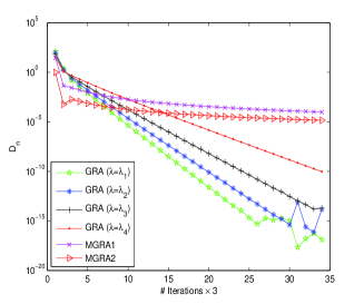
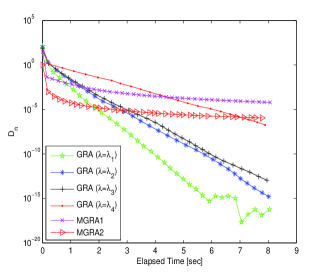
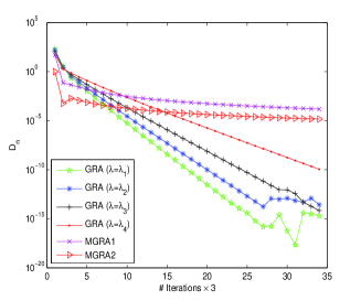
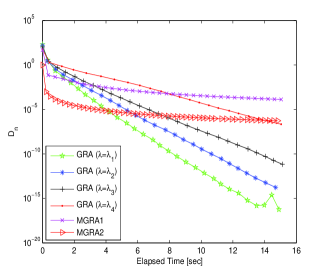
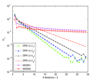
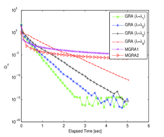
In this section, we present some experiments to illustrate the numerical behavior of Algorithm 3.1 (GRA) and also to compare with other algorithms. Two algorithms used here to compare are MGRA1 (V2018, , Algorithm 4.1) and MGRA2 (V2018, , Algorithm 4.2). The convergence of these algorithms are established under a same assumption of strong pseudomonotonicity of bifunction, while the Lipschitz-type condition are only for Algorithm 3.1 and MGRA1. In order to show the computational performance of the algorithms, we describe the behavior of the sequence $D_{n}=||x_{n}-{\rm prox}_{\lambda f(x_{n},.)}(x_{n})||^{2},~{}n=0,~{}1,2,\ldots$ when number of iterations (# Iterations) is performed or execution time (Elapsed Time) in the second elapses. Noting that $D_{n}=0$ iff $x_{n}$ is the solution of the considered problem.
Considering a generalization of the Nash-Cournot oligopolistic equilibrium model in CKK2004 ; FP2002 with the affine price and fee-fax functions. Assume that there are $m$ companies that produce a commodity. Let $x$ denote the vector whose entry $x_{j}$ stands for the quantity of the commodity produced by company $j$. We suppose that the price $p_{j}(s)$ is a decreasing affine function of $s$ with $s=\sum_{j=1}^{m}x_{j}$, i.e., $p_{j}(s)=\alpha_{j}-\beta_{j}s$, where $\alpha_{j}>0$, $\beta_{j}>0$. Then the profit made by company $j$ is given by $f_{j}(x)=p_{j}(s)x_{j}-c_{j}(x_{j})$, where $c_{j}(x_{j})$ is the tax and fee for generating $x_{j}$. Suppose that $C_{j}=[x_{j}^{\min},x_{j}^{\max}]$ is the strategy set of company $j$, then the strategy set of the model is $C:=C_{1}\times C_{2}\times...\times C_{m}$. Actually, each company seeks to maximize its profit by choosing the corresponding production level under the presumption that the production of the other companies is a parametric input. A commonly used approach to this model is based upon the famous Nash equilibrium concept. We recall that a point $x^{*}\in C=C_{1}\times C_{2}\times\cdots\times C_{m}$ is an equilibrium point of the model if

$$f_{j}(x^{*})\geq f_{j}(x^{*}[x_{j}])\ \forall x_{j}\in C_{j},\ \forall j=1,2,\ldots,m,$$

where the vector $x^{*}[x_{j}]$ stands for the vector obtained from $x^{*}$ by replacing $x^{*}_{j}$ with $x_{j}$. By taking $f(x,y):=\psi(x,y)-\psi(x,x)$ with $\psi(x,y):=-\sum_{j=1}^{m}f_{j}(x[y_{j}])$, the problem of finding a Nash equilibrium point of the model can be formulated as:

$$\mbox{Find}~{}x^{*}\in C~{}\mbox{such that}~{}f(x^{*},x)\geq 0~{}\forall x\in C.$$

Now, assume that the tax-fee function $c_{j}(x_{j})$ is increasing and affine for every $j$. This assumption means that both of the tax and fee for producing a unit are increasing as the quantity of the production gets larger. In that case, the bifunction $f$ can be formulated in the form

$$f(x,y)=\left\langle Px+Qy+q,y-x\right\rangle,$$

where $q\in\Re^{m}$ and $P,~{}Q$ are two matrices of order $m$ such that $Q$ is symmetric positive semidefinite and $Q-P$ is symmetric negative semidefinite. The bifucntion $f$ satisfies the Lipschitz-type condition with $c_{1}=c_{2}=||P-Q||/2$. In order to assure that all the algorithms can work, the datas here are generated randomly such that $Q-P$ is symmetric negative definite. In this case, the bifunction $f$ is strongly pseudomonotone. We perform the numerical computations in $\Re^{m}$ with $m=100,~{}200,~{}300$; the feasible set is $C=[-2,5]^{m}$; the starting point $x_{1}=\bar{x}_{0}$ are generated randomly in the interval $[0,1]$. The datas are generated as follows: All the entries of $q$ is generated randomly and uniformly in $(-2,2)$ and the two matrices $P,~{}Q$ are also generated randomly such that their conditions hold. All the optimization subproblems are effectively solved by the function quadprog in Matlab 7.0.
We take $\lambda=\lambda_{i}:=\frac{p_{i}\varphi}{4c_{1}}$, $i=1,2,3,4$ for Algorithm 3.1 (GRA), where $p_{1}=0.9,~{}p_{2}=0.7,~{}p_{3}=0.5,~{}p_{4}=0.3$ and $\lambda_{n}=\beta_{n}=\frac{1}{n+1}$ for the MGRA1 and MGRA2. The numerical results are shown in Figs. 2 - 6. In view of these figures, we see that Algorithm 3.1 works better than other algorithms in both execution time and number of iterations.

Figure 1: $D_{n}$ and # Iterations (in $\Re^{100}$)

Figure 2: $D_{n}$ and Time (in $\Re^{100}$)

Figure 3: $D_{n}$ and # Iterations (in $\Re^{200}$)

Figure 4: $D_{n}$ and Time (in $\Re^{200}$)

Figure 5: $D_{n}$ and # Iterations (in $\Re^{300}$)

Figure 6: $D_{n}$ and Time (in $\Re^{300}$)

References

• (1) Anh, P.N., Hieu, D.V.: Multi-step algorithms for solving EPs. Math. Model. Anal. 23, 453-472 (2018)
• (2) Bauschke, H. H., Combettes, P. L.: Convex Analysis and Monotone Operator Theory in Hilbert Spaces. Springer, New York (2011)
• (3) Blum, E., Oettli, W.: From optimization and variational inequalities to equilibrium problems. Math. Student. 63, 123–145 (1994)
• (4) Contreras, J., Klusch, M., Krawczyk, J. B.: Numerical solutions to Nash-Cournot equilibria in coupled constraint electricity markets. IEEE Trans. Power Syst. 19, 195-206 (2004)
• (5) Facchinei, F., Pang, J. S.: Finite-Dimensional Variational Inequalities and Complementarity Problems. Springer, Berlin (2002)
• (6) Flam, S. D., Antipin, A. S.: Equilibrium programming and proximal-like algorithms. Math. Program. 78, 29-41 (1997)
• (7) Hieu, D. V., Cho, Y. J., Xiao, Y-B.: Modified extragradient algorithms for solving equilibrium problems. Optimization (2018). DOI: 10.1080/02331934.2018.1505886
• (8) Hieu, D. V.: An inertial-like proximal algorithm for equilibrium problems. Math. Meth. Oper. Res. (2018). DOI:10.1007/s00186-018-0640-6
• (9) Hieu, D. V.: New inertial algorithm for a class of equilibrium problems. Numer. Algor. (2018). DOI:10.1007/s11075-018-0532-0
• (10) Hieu, D. V.: Convergence analysis of a new algorithm for strongly pseudomontone equilibrium problems. Numer. Algor. 77, 983-1001 (2018)
• (11) Hieu, D. V.: An extension of hybrid method without extrapolation step to equilibrium problems. J. Ind. Manag. Optim. 13, 1723–1741 (2017)
• (12) Konnov, I. V. : Application of the proximal point method to non-monotone equilibrium problems. J. Optim. Theory Appl. 119, 317-333 (2003)
• (13) Konnov, I. V.: Equilibrium Models and Variational Inequalities. Elsevier, Amsterdam (2007)
• (14) Korpelevich, G.M.: The extragradient method for finding saddle points and other problems. Ekonomikai Matematicheskie Metody. 12, 747-756 (1976)
• (15) Lyashko, S. I. , Semenov, V. V.: A new two-step proximal algorithm of solving the problem of equilibrium programming. In Optimization and Its Applications in Control and Data Sciences. Springer, Switzerland 115, 315-325 (2016)
• (16) Malitsky, Y.: Golden ratio algorithms for variational inequalities. (2018). https://arxiv.org/abs/1803.08832
• (17) Moudafi, A.: Proximal point algorithm extended to equilibrum problem. J. Nat. Geometry, 15, 91-100 (1999)
• (18) Muu, L. D., Oettli, W.: Convergence of an adative penalty scheme for finding constrained equilibria. Nonlinear Anal. TMA 18, 1159–1166 (1992)
• (19) Quoc, T. D., Muu, L. D., Nguyen, v: Extragradient algorithms extended to equilibrium problems. Optimization 57, 749-776 (2008)
• (20) Santos, P., Scheimberg, S.: An inexact subgradient algorithm for equilibrium problems. Comput. Appl. Math. 30, 91-107 (2011)
• (21) Strodiot, J. J., Nguyen, T. T. V., Nguyen, V. H.: A new class of hybrid extragradient algorithms for solving quasi-equilibrium problems. J. Glob. Optim. 56, 373-397 (2013)
• (22) Vinh, N. T.: Golden ratio algorithms for solving equilibrium problems in Hilbert spaces. (2018). https://arxiv.org/abs/1804.01829