On modeling for Kerr black holes: Basis learning, QNM frequencies, and spherical-spheroidal mixing coefficients

Abstract

Models of black hole properties play an important role in the ongoing direct detection of gravitational waves from black hole binaries. One important aspect of model based gravitational wave detection, and subsequent estimation of source parameters, are the low level modeling of information related to perturbed Kerr black holes. Here, we present new phenomenological methods to model the analytically understood gravitational wave spectra (quasi-normal mode frequencies), and harmonic structure of Kerr black holes (mixing coefficients between spherical and spheroidal harmonics). In particular, we present a greedy-multivariate-polynomial (GMVP) regression method and greedy-multivariate-rational (GMVR) regression method for the automated modeling of polynomial and rational functions respectively. GMVR is a quasi-linear numerical method for interpolating rational functions. It therefore represents a solution to Runge’s phenomenon. GMVP is used to develop a model for QNM frequencies that explicitly enforces consistency with the extremal Kerr limit. GMVR is used to develop a model for harmonic mixing coefficients that extends previous results to dominant multipoles with $\ell\leq 5$. Both models are the first of their kind to consider black hole spin to vary between -1 and 1, thus naturally connecting the pro and retrograde modes. We discuss the potential use of these models in current and future gravitational wave signal modeling.

I Introduction

In the coming years, expectations for frequent Gravitational wave (GW) detections of increasing signal-to-noise ratio (SNR) are high Abbott et al. (2016a, c). Concurrent with Virgo, the Advanced LIGO (aLIGO) detectors will enter their third observing run in approximately early 2019. During this period, a few to dozens of binary black hole (BH) signals are likely to be detected Abbott et al. (2016c); Abbott2018OS. In this context, signal detection and subsequent inference of physical parameters hinges upon efficient models for source properties and dynamics Abbott et al. (2017). Most prominently, there is ongoing interest in efficient and accurate signal models for binary BH inspiral, merger and ringdown (IMR) Blackman et al. (2017); London et al. (2018b); Hannam et al. (2014). As the merger of isolated BHs is expected to result in a perturbed Kerr BH, there is related interest in having computationally efficient models for perturbative parameters, namely those that enable evaluation of the related ringdown radiation Berti et al. (2006).

In particular, a perturbed Kerr BH (e.g. resulting from binary BH merger) will have GW radiation that rings down with characteristic dimensionless frequencies, $\tilde{\omega}_{\ell mn}=\omega_{\ell mn}+i/\tau_{\ell mn}$, where $\omega_{\ell mn}$ is the central frequency of the ringing, and $1/\tau_{\ell mn}$ is the damping rate. These discrete frequencies have associated radial and spatial functions which are spheroidal harmonic in nature Leaver (1985). Together, these harmonic functions and frequencies constitute the Quasi-Normal Mode (QNM) solutions to Einstein’s equations. Specifically, they are the eigen-solutions of the source free linearized Einstein’s equations (i.e. Teukolsky’s equations Teukolsky (1972)) for a perturbed BH with final mass, $M_{f}$, and dimensionless final spin, $j_{f}$. These solutions allow gravitational radiation from generic perturbations to be well approximated by a spectral (multipolar) sum which combines the complex QNM amplitude, $A_{\ell mn}$, with the spin $-2$ weighted -2 spheroidal harmonics, ${}_{-2}S_{\ell mn}$.

$$h =h_{+}-i\,h_{\times}$$ (1)

$$=\frac{1}{r}\sum_{\ell mn}A_{\ell mn}\;e^{i\,\tilde{\omega}_{\ell mn}t}\;_{-2}S_{\ell mn}(j_{f}\tilde{\omega}_{\ell mn},\theta,\phi)$$

$$=\frac{1}{r}\sum_{\bar{\ell}\bar{m}}h_{\bar{\ell}\bar{m}}(t)\;_{-2}Y_{\bar{\ell}\bar{m}}(\theta,\phi)\;.$$

In the first and second lines of Eqn. (1), we relate the observable GW polarizations, $h_{+}$ and $h_{\times}$, to the analytically understood morphology of the time domain ringdown waveform. Here, the labels $\ell$ and $m$ are polar and azimuthal eigenvalues of Teukolsky’s angular equations, where total mass and the speed of light are set to unity (i.e. $M=c=1$). Note that barred indices, namely $\bar{\ell}$ and $\bar{m}$, refer to spherical harmonics of spin weight -2, leaving the unbarred indices to refer to the spheroidals. In the third line of Eqn. (1), we represent $h$ in terms of spherical harmonic multipoles. This latter form is ubiquitous for the development and implementation of IMR signal models for binary BHs.

Towards the development of these models, Eqn. (1) enters in many incarnations. In the Effective One Body (EOB) formalism, $h_{\bar{\ell}\bar{m}}$ is modeled such that, after its peak (near merger), the effective functional form reduces (asymptotically) to Eqn. (1)’s second line Cotesta et al. (2018); Buonanno & Damour (2000); Bohé et al. (2017); Pan et al. (2014); Bohé et al. (2017); Nagar et al. (2018). This view currently comes with the added assumption that ${{}_{-2}}S_{\ell mn}={{}_{-2}}Y_{\ell m}$, where ${{}_{-2}}Y_{\ell m}$ are the spins weighted -2 spherical harmonics. Only where $j_{f}\tilde{\omega}_{\ell mn}=0$ do ${}_{-2}S_{\ell mn}(0,\theta,\phi)={{}_{-2}}Y_{\ell m}(\theta,\phi)$, which makes equating the spherical and spheroidal harmonics approximate at best for general values of $j_{f}\tilde{\omega}_{\ell mn}$. The consequences of that approximation, in particular the mixing between spherical and spheroidal harmonics, are discussed in reference London et al. (2014); Berti & Klein (2014); London (2018); Kelly:2012nd. This approximation also applies to the Phenom models, where the frequency domain multipoles, $\tilde{h}_{\bar{\ell}\bar{m}}(f)$, are constructed such that their high frequency behavior is consistent with Eqn. (1) in the time domain Hannam et al. (2014); London et al. (2018b); Khan et al. (2016); Schmidt et al. (2015); Mehta:2017jpq; Khan:2018fmp.

Both Phenom and EOB approaches either use phenomenological models of remnant BH mass and spin to interpolate over tables of QNM frequencies, or phenomenological models for QNM frequencies are used directly. Either approach typically incurs less computational cost that the direct numerical calculation of QNM frequencies, which may involve, for example, the solving of continued fraction equations Leaver (1985). In the case of the higher multipole model PhenomHM and its derivative models, fits for the QNM frequencies are used in the process of mapping $\tilde{h}_{22}(f)$ into other $\tilde{h}_{\bar{\ell}\bar{m}}(f)$ London et al. (2018b). In that setting, it is demonstrated that QNM frequencies are linked to the amplitude and phase of each $h_{\bar{\ell}\bar{m}}$ in not only ringdown, but also merger and late inspiral, as is implied by the source’s causal connectedness pre and post merger.

For models that assist tests of the No-Hair Theorem (e.g. Berti et al. (2006); London (2018); Carullo et al. (2018)), and thereby only include precise ringdowns, the perspective of Eqn. (1)’s second and third lines are used to write each spherical harmonic multipole moment as

$$h_{\bar{\ell}\bar{m}}=\frac{1}{r}\sum_{\ell mn}\,A_{\ell mn}e^{i\tilde{\omega}_{\ell mn}t}\sigma_{\bar{\ell}\bar{m}\ell mn}$$ (2)

where, the spherical-spheroidal mixing coefficient, $\sigma_{\bar{\ell}\bar{m}\ell mn}$, is

$$\sigma_{\bar{\ell}\bar{m}\ell mn}=\int_{\Omega}{{}_{-2}S}_{\ell mn}\,{{}_{-2}}Y^{*}_{\bar{\ell}\bar{m}}\,\mathrm{d}\Omega\;.$$ (3)

In Eqn. (3), $*$ denotes complex conjugation, and $\Omega$ is the standard solid angle in spherical polar coordinates.

In practice, using Eqn. (2) is computationally efficient: Whereas the calculation of each ${{}_{-2}S}_{\ell mn}$ involves a series solution which slowly converges for $j_{f}$ near unity, the calculation of each ${{}_{-2}Y}_{\bar{\ell}\bar{m}}$ is achieved using closed form expressions. It is therefore efficient to use accurate models for $\sigma_{\bar{\ell}\bar{m}\ell mn}$ to avoid convergence issues. These can then be used directly to calculate $h_{\bar{\ell}\bar{m}}$ via Eqn. (2), and thereby the GW polarizations via Eqn. (1).

In this combined context, it is clear that the modeling of QNM frequencies, $\tilde{\omega}_{\ell mn}$, and spherical-spheroidal mixing coefficients, $\sigma_{\bar{\ell}\bar{m}\ell mn}$, are relevant for a range of GW signal models. While models for $\tilde{\omega}_{\ell mn}$ and $\sigma_{\bar{\ell}\bar{m}\ell mn}$ are present in the literature (e.g. Berti et al. (2006); Berti & Klein (2014); Cook:2014cta), there exist minor shortcomings which we wish to address here.

For both the QNM frequencies and the spherical-sphoidal mixing coefficients, we present the first models which treat QNMs rotating with and against the rotation of the BH as being a part of a single solution parameterized by dimensionless BH spin ranging from -1 to 1. This perspective reflects the empirical observation that the remnant spin of binary BH mergers smoothly connects regions of positive and negative spin relative to the direction of the initial oribital angular momentum Husa:2015iqa; London (2018).

For the QNM frequencies, it is well known that for nearly extremal BHs (i.e. $j_{f}\rightarrow 1$) some of the frequencies have zero-damping (i.e. $\tau_{\ell mn}\rightarrow\infty$) Yang et al. (2013); Zimmerman & Mark (2016). In the context of GW data analysis, where source parameters are estimated using routines which sample over the space of all possible BH masses and spins, it is useful to have accurate physical behavior in the extremal limit Abbott et al. (2016b). Like Ref. Cook:2014cta, we present models for $\tilde{\omega}_{\ell mn}$ that explicitly account for zero-damping in the extremal Kerr limit. The models presented here go further by applying outside of the nearly extremal Kerr regime while also accounting for non-zero-damping in modes such as $(\ell,m,n)=(2,1,0)$ and $(3,2,0)$Yang et al. (2013).

For the modeling of $\sigma_{\bar{\ell}\bar{m}\ell mn}$, we note that the models of Ref. Berti & Klein (2014) do not appear to include the QNMs which rotate counter to the BH spin direction (i.e. “mirror-modes”). Here these QNM are explicitly modeled on a continuation of the positive spin line to negative spin.

In parallel, the methods for modeling $\tilde{\omega}_{\ell mn}$ and $\sigma_{\bar{\ell}\bar{m}\ell mn}$ have been dispersed: different phenomenological techniques have been used under no coherent framework. Here we will present linear modeling techniques, namely the greedy-multivariate-polynomial (GMVP) and greedy-multivariate-rational (GMVR) algorithms, in which model terms are iteratively learned with no initial guess. The description of GMVP given here is complementary to similar algorithms used to model QNM excitation amplitudes, $A_{\ell mn}$, as present in reference Carullo et al. (2018); London (2018); London et al. (2014). As we will discuss, the GMVR algorithm is an iterative approach to the (pseudo) linear modeling of multivariate rational functions, wherein iterations of linear inversions are used to refine the ultimately non-linear model.

In the rudimentary form presented here, both GMVP and GMVR are intended for use with low noise data (e.g. the results of analytic calculations), and each employs a reverse (or negative) greedy algorithm to counter over modeling Field et al. (2011); Caudill et al. (2012). As the underlying process for GMVP and GMVR is stepwise regression, highly correlated basis vectors (i.e. polynomial terms) are handled via an approach we will call degree tempering. It will be demonstrated that these approaches are readily capable of modeling the complex valued $\tilde{\omega}_{\ell mn}$ and $\sigma_{\bar{\ell}\bar{m}\ell mn}$. Results suggest that the versions of GMVP and GMVR presented here may apply in instances where training data are approximately noiseless, and an initial guess is difficult to obtain. Both algorithms are publicly available in Python via Ref. London et al. (2018a). While this paper’s fits for the QNM frequencies and mixing coefficients are presented in Equations (26)–(34) and Equations (35)–(46) respectively, we encourage the reader to use the fits implemented in Ref. London et al. (2018a): positive.physics.cw181003550 (QNM frequencies) and in positive.physics.ysprod181003550 (mixing coefficients).

The plan of the paper is as follows. In section Section (II), we outline the GMVP and GMVR algorithms. In Section (III), we demonstrate the application of each algorithm. We first consider the application of GMVP to the modeling of QNM frequencies. We then consider the application of GMVR to the modeling of spherical-spheroidal mixing coefficients. Quantitative comparisons are made between our models and those presented in Refs. Berti et al. (2006); Berti & Klein (2014). In Section (IV), we review the effectiveness of GMVP and GMVR, and we discuss current and potential applications for these methods.

II Methods

Within the topic of regression, linear regression has particular advantages. Its matrix based formulation can be computationally efficient, and it does not require initial guesses for model parameters. Perhaps most intriguingly, the formal series expansions of smooth functions support linear and rational models (e.g. Padé approximants) that have application to many datasets. With this in mind, here, we will develop algorithms for the linear (polynomial and rational) modeling of scalar functions (real or complex) of many variables.

If we consider a scalar function, $f$, of $N$ variables sampled in $j$, $\vec{x}_{j}=\{x_{\alpha j}\}_{\alpha=0}^{N}$, then $f(\vec{x}_{j})$ can be represented (possibly inaccurately) as a sum over $K$ linearly independent basis functions, $\phi_{k}(\vec{x}_{j})$:

$$f({\vec{x}}_{j})\;=\;\sum_{k=0}^{K}\;\mu_{k}\,\phi_{k}(\vec{x}_{j})\;.$$ (4)

The central player in Eqn. (4) is the set of basis coefficients $\mu_{k}$. Typically, one chooses or derives $\phi_{k}(\vec{x}_{j})$ to capture inherent features of $f(\vec{x}_{j})$. With $\phi_{k}(\vec{x}_{j})$ assumed to be known, the linear representation (namely Eqn. 4) is lastly defined the set of $\mu_{k}$.

From here it is useful to note that Eqn. (4) has a linear homogeneous matrix form. In particular, defining ${U}_{jk}=\phi_{k}(\vec{x}_{j})$, $f_{j}=f(\vec{x}_{j})$ and $\vec{f}=\hat{U}\;\vec{\mu}$, implies that

$$\vec{\mu}=\hat{P}\;\vec{f}\;,$$ (5)

where

$$\hat{P}=\left(\hat{U}^{*}\hat{U}\right)^{-1}\hat{U}^{*}$$ (6)

is the pseudo-inverse Moore (1920); Penrose (1955) of $\hat{U}$, which exists if $\hat{U}^{*}\hat{U}$ is nonsingular. Here “$*$” denotes the conjugate transpose.

Equations (4), and related discussion through Eqn. (6) illustrate the most rudimentary solution to the linear modeling problem. However, there are many ways to expand upon and refine the solution presented thus far. In the following subsections we will consider two such approaches. First we will consider the general polynomial modeling of multivariate scalar functions. This will encompass the GMVP algorithm. Second, we will build upon the GMVP approach by considering models of rational functions (polynomials divided by polynomials). To consider these two approaches in a largely automated way (i.e. where the set of possible basis functions is known, but the select basis functions ultimately used are learned), we will make use of the greedy algorithm approach Field et al. (2011); GVK022791892; 1978AnSta; Pandit84.

II.1 A Generic Greedy Algorithm

While we most often want a single model for a given dataset (e.g. some approximation of $\vec{f}$ from numerical calculation or experiment), there are often many more modeling choices than desired. In particular, if we refer to our set of all possible basis functions as our “symbol space”, then the problem of determining how many, and which basis vectors (i.e. symbols) to use is a problem of combinatoric complexity.

A well known method for finding an approximate solution to this problem is the so-called “greedy” algorithm (e.g. Field et al. (2011); GVK022791892): We will iteratively construct models with increasing number of symbols. The process begins by finding the single symbol (basis vector) that yields the most accurate model in the sense of minimizing the least-squares error. That encompasses the first iteration of a process in which we will greedily add symbols to our model. In each subsequent iteration, remaining symbols are added to the model one at a time, resulting in many trial models, each with its own representation error. The trial model with smallest representation error is kept for the next greedy iteration. In this way, a list of optimal model symbols is learned. This forward greedy process ends when the model accuracy, and/or changes thereof, passes a previously specified threshold. This rough algorithmic picture is encapsulated by Alg. 1.          

Algorithm 1 A positive (forward) greedy algorithm, PGREEDY. Note that a required input, $\mathcal{A}$, is a function that takes in a list of basis symbols, and outputs an estimator of fit error (e.g. $L^{2}$ norm). In this setting, $\mathcal{A}$ is assumed to have access to peripheral information, such as the training data.

1:Input: $\{{\bm{\lambda}}_{bulk}=\text{basis symbols}$, $\mathcal{A}=\text{action}$, $tol=\text{greedy tolerance}\}$

2:Define empty list of kept symbols: ${\bm{\lambda}}_{kept}=\{\}$

3:Initialize estimator value and loop boolean: $\epsilon_{last}=\mathrm{inf}$, $done=\text{False}$

4:while not $done$ do

5:    $\epsilon_{min}=\epsilon_{last}$

6:    for  ${\bm{\lambda}}$ in ${\bm{\lambda}}^{bulk}$  do

7:       ${\bm{\lambda}}_{trial}={\bm{\lambda}}_{kept}\cup{\bm{\lambda}}$              (add ${\bm{\lambda}}$ to ${\bm{\lambda}}_{kept}$)

8:       $\epsilon=\mathcal{A}({\bm{\lambda}}_{trial})$                  (action returns fit error)

9:       if  $\epsilon<\epsilon_{min}$  then

10:          $\epsilon_{min}=\epsilon$                    (store trial min)

11:          ${\bm{\lambda}}_{min}={\bm{\lambda}}_{trial}$

12:       end if

13:    end for

14:    $done=|\epsilon_{min}-\epsilon_{last}|<tol$

15:    if  not $done$  then

16:       $\epsilon_{last}=\epsilon_{min}$

17:       ${\bm{\lambda}}_{kept}={\bm{\lambda}}_{kept}\cup{\bm{\lambda}}_{min}$           (update kept symbols)

18:    end if

19:end while

20:Output: $\{{\bm{\lambda}}_{kept}\}$ (the Greedy Basis)

The very similar “negative” greedy algorithm removes model symbols until representation error increases beyond a specified threshold.

II.2 Greedy Multivariate Polynomial Fitting

The study of smooth scalar functions (e.g. $f(\vec{x})$) often centers about the Taylor series expansion. In that instance, it is clear that any infinitely differentiable scalar function of many variables can be represented in terms of its derivatives by

$$f(\vec{x}+\vec{h}) =e^{\vec{x}\cdot\vec{\nabla}^{\prime}}\,f(\vec{x}\,^{\prime})|_{\vec{x}\,^{\prime}=\vec{h}}$$ (7)

$$\approx\sum_{k=0}^{K}\,\frac{1}{k!}\,(\vec{x}\cdot\vec{\nabla}^{\prime})^{k}\,f(\vec{x}\,^{\prime})|_{\vec{x}\,^{\prime}=\vec{h}}$$

From the first to second line of Eqn. (7), we have used the definition of the exponential function (i.e. its series expansion). In the second line, the equality has been replaced by an approximation as we have limited the linear representation to $K+1$ terms.

This latter point is key to the perspective of GMVP: given training data thought to be related to a smooth multivariate function, it may, particularly on small scales, be well approximated by a truncated series expansion in an appropriate coordinate basis.

Algorithm 2 GMVP, a degree tempered stepwise algorithm for multivariate polynomial modeling of scalar data.

1:Input: $\{x,f,$max_degree = 6$,tol\}$

2:Define, ${\bm{\lambda}}_{bulk}$, the bulk symbol space, to be the set of all multinomial combinations of basis vectors up to a predefined maximum order.

3:Define $\mathcal{A}_{\texttt{GMVP}{}}$ according to Alg. (3).

4:Given $max\_degree$, define, ${D}$, a list of allowed polynomial degrees (e.g. $\{0,1,2,3,4,5,6\}$)

5:for $d$ in ${D}$  do

6:    Define ${\bm{\lambda}}_{bulk}^{(d)}$ as all symbols from ${\bm{\lambda}}_{bulk}$ with degree less than or equal to current degree: ${\bm{\lambda}}^{(d)}_{bulk}$

7:    Using ${\bm{\lambda}}_{bulk}^{(d)}$, apply Alg. (1), PGREEDY, with $\mathcal{A}_{\texttt{GMVP}{}}$ to get symbol subset, ${\bm{\lambda}}^{(d)}_{opt}$ and estimator val, $\epsilon^{(d)}_{opt}$

8:    if  $|\epsilon^{(d)}_{opt}-\epsilon^{(d-1)}_{opt}|<tol$  then

9:       break

10:    end if

11:end for

12:Output: ${\bm{\lambda}}^{(d)}_{opt}$

Eqn. (7)’s truncated expansion happens to be a polynomial in at most $N$ variables. In this setting, the uncertainty of which and how many basis terms to include makes this a problem ripe for the application of linear modeling driven by a greedy process, namely Eqn. (5) and Alg. (1) .

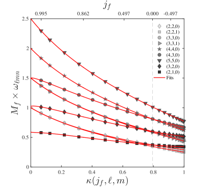
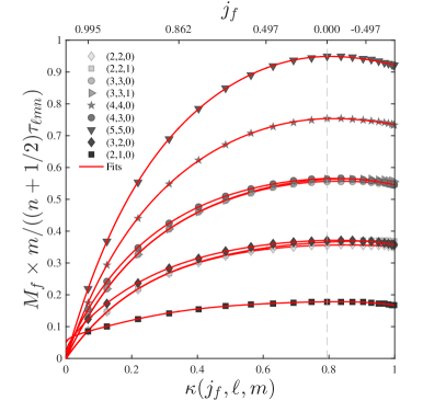
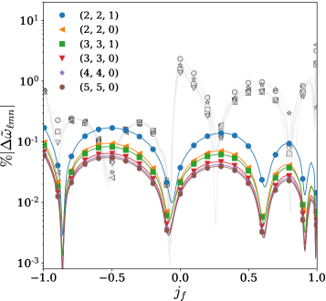
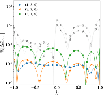
Figure 1: Fits of dimensionless QNM central frequencies (solid lines) along with select numerical values (grey markers) computed using Leaver’s method Leaver (1985). Before the application of $\kappa(\j{})$, points are spaced between - 0.995 and 0.995 according to 0.995 times the $\sin$ of a fiducial angle which is uniformly spaced between $-\pi/2$ and $\pi/2$. Values of $\j{}$ are shown in the upper axis for $\kappa$ at $l=m$. The grey dashed line marks the value of $\kappa$ where $\j{}=0$. Fits of dimensionless QNM decay rates (solid lines) along with select numerical values (grey markers) computed using Leaver’s method Leaver (1985). (Bottom) Percentage absolute residual errors for fits of dimensionless QNM frequencies,, $\tilde{\omega}_{\ell mn}$ along with select numerical values (colored markers) computed using Leaver’s method Leaver (1985). For comparison, residuals using the models in Ref. Berti et al. (2006) are shown in gray.

Here, the basis symbols required by Alg. (1) are the multinomial terms in Eqn. (7). Each term is an element of the tensor-product of the power-sets of each model dimension. That is ${\bm{\lambda}}_{bulk}=\{x_{0},x_{1}..x_{N},...x_{0}^{1},x_{0}^{2},x_{0}^{3},...,(x_{0}^{K}x_{1}^{K}...x_{N}^{K})\}$. Note that in practice it may be useful to encode elements of ${\bm{\lambda}}_{bulk}$ with strings representing their constituents (e.g. $x_{0}x_{0}x_{1}x_{2}x_{2}x_{4}$ could be represented by the string “001224”). This provides a way of bijectively mapping between symbols and numerical basis vectors.

The action, $\mathcal{A}({\bm{\lambda}}_{trial})$, required by Alg. (1) encompasses the evaluation of Eqn. (5) to solve for the basis coefficients, $\mu_{k}$, and the calculation of the modeling error. An explicit sketch of this is given by Alg. (3).

The combination of these two ideas alone results in an algorithm prone to a deficit of stepwise methods: the algorithm may confuse correlated basis vectors (e.g. $x^{2}$ may be confused with $x^{4}$). To counter this, we may incrementally increase, or temper, the maximum allowed multinomial degree. For example, when iterating through allowed degrees, if the current maximum degree is 3, then degree 4 terms, such as $x_{0}x_{1}x_{3}^{2}$, will not be considered within the space of model symbols. The degree tempering process halts when increasing the maximum allowed degree has no significant effect on model representation error.

The combination of degree tempering with the greedy approach results in the GMVP algorithm as presented in Alg. (2).

II.3 Greedy Multivariate Rational Fitting

Despite the apparent universality of Eqn. (7), there are many cases where $K$ must be orders of magnitude greater than 1 in order for $\vec{f}$ to be accurately represented by a low order multinomial. Worst, in cases where the underlying dataset is best described by a rational function, no polynomial of the same family describing the numerator and denominator will yield satisfactory results in low order (e.g. the well known “Runge’s phenomenon” Epperson (1987)). In general, the optimal polynomial basis may not be clear, and so a more general set of ansatzes may be of use.

Of the simplest of such ansatzes are rational functions of the form

$$f(\vec{x})=\bar{\mu}+\bar{\sigma}_{f}\;\frac{\sum_{r=0}^{R}a_{r}\,\phi_{r}(\vec{x})}{1-\sum_{v=1}^{V}b_{v}\,\phi_{v}(\vec{x})}\;,$$ (8)

where $\bar{\mu}$ is the additive mean of $f(\vec{x})$, and $\bar{\sigma}_{f}$ is the standard deviation of $f(\vec{x})$, and $\phi_{k}$ are the multinomials basis functions considered in the previous section. Note that, in Eqn. (8), the sum over $v$ does not include the constant term associated with $\phi_{0}$.

While it is tempting to embrace Eqn. (8)’s $f({\vec{x}})$ as a nonlinear function and so resort to nonlinear modeling methods, a reformulation reveals an underlying linear structure Press et al. (1992). Namely, if we let

$$g=(f-\bar{\mu})/\bar{\sigma}_{f}$$ (9)

then algebraic manipulation of Eqn. (8) allows

$$g=\sum_{r=0}^{R}a_{r}\,\phi_{r}(\vec{x})+g\,\sum_{v=1}^{V}b_{v}\,\phi_{v}(\vec{x})\;.$$ (10)

We are free to relabel the indices such that Eqn. (10) is manifestly linear in a single index. At this stage, we will also explicitly consider the $j^{\mathrm{th}}$ samples of the domain, and so refer to (e.g.) $\vec{x}$ as $\vec{x}_{j}$.

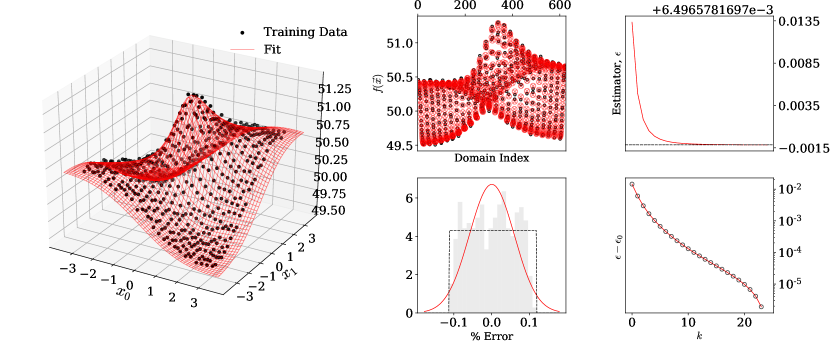
Figure 2: Standard summary plot for Greedy Multivariate Rational fitting algorithm (GMVR) as implemented in London et al. (2018a). (left) 3D plot of training data (black dots) and final fit (red mesh). (center top) Same as left most panel, but in index space. (center bottom) Percent residual error with respect to validation data (grey blocks) along with uniform (black) and gaussian (red) fits to error. The validation data were generated in the same manner as the training data. (top right) convergence of the $L^{2}$ norm during iterative refinement. (bottom right) Same as top right, but on log scale, where $\epsilon_{0}$ is the value of $\epsilon$ at the final $k^{\mathrm{th}}$ iteration of refinement.

These adjustments of perspective result in

$$g_{j}=\sum_{k=0}^{R+V}\,z_{k}\,\psi_{k}(\vec{x}_{j})\;,$$ (11)

where

$$z_{k}=\left\{\begin{array}[]{cc}a_{k},&\text{for }0\leq k\leq R\\ b_{k},&\quad\;\;\;\text{for }R+1\leq k\leq R+V\end{array}\right\}$$ (14)

and

$$\psi_{k}(\vec{x}_{j})=\left\{\begin{array}[]{cc}\phi_{k}(\vec{x}_{j}),&\text{for }0\leq k\leq R\\ \phi_{k}(\vec{x}_{j})\,g_{j},&\quad\;\;\;\text{for }R+1\leq k\leq R+V\end{array}\right\}$$ (17)

Recalling Equations (5)–(6), it follows that the coefficients of interest ($a_{k}$ and $b_{k}$), may be estimated according to

$$\vec{\alpha}=\hat{P}\;\vec{g}\;.$$ (18)

where, $\hat{P}$ is the pseudo-inverse of the matrix whose elements are $\psi_{k}(\vec{x}_{j})$, $\vec{\alpha}=(z_{0},z_{1},...z_{R+V-1},z_{R+V})$, and $\vec{g}=(g_{0},g_{1},...g_{R+V-1},g_{R+V})$.

However, we note that $\hat{P}$ depends nontrivially on $g$, and is therefore susceptible to noise in the training data. Let us briefly consider the effect of zero-mean noise on $g$, e.g. $g\rightarrow g+n$. In this, it may be that shown that $n$ may be entirely relegated to $\hat{P}$. It is in this sense that Eqn. (18) is insufficient to generally solve for $\vec{\alpha}$, as $\hat{P}$ may be adversely affected by noise.

The key to robustly solving for $\vec{\alpha}$ lies in iterative refinement Press et al. (1992). Specifically, we note that Eqn. (10) may be modified to iteratively minimize the impact of numerical noise on $\hat{P}$. That is, to reduce the impact of noise on $\hat{P}$, we are free to calculate it using model evaluations of $g$ rather than the original (noisy) training data. If we define $g^{(0)}=g$ (i.e. $g$ is the training data), with $\hat{P}=\hat{P}(\vec{g}^{\,(n)})$, then Eqn. (18) generalizes to

$$\vec{\alpha}^{(n+1)}=\hat{P}(\vec{g}^{\,(n)})\,\vec{g}^{(0)}\;.$$ (19)

In practice, one solves Eqn. (19) for $\vec{\alpha}^{(n+1)}$, and then uses the related $a_{r}^{(n+1)}$ and $b_{v}^{(n+1)}$ to calculate $g^{(n+1)}$ via

$$g^{(n+1)}=\frac{\sum_{r=0}^{R}a^{(n+1)}_{r}\,\phi_{r}(\vec{x})}{1\;-\;\sum_{v=1}^{V}b^{(n+1)}_{v}\,\phi_{v}(\vec{x})}\;.$$ (20)

Subsequently, $g^{(n+1)}$ is then fed back into Eqn. (19) for further refinement. The refinement process is to terminate when a measure of model error (e.g. the $L^{2}$ norm $||g^{(0)}-g^{(n)}||$) passes a predetermined threshold.

Algorithm 3 $\mathcal{A}_{\texttt{GMVP}}$, the action for GMVP. Model calculation given basis symbols, and output of model error estimate.

1:Input: ${\bm{\lambda}}_{trial}$

2:Calculate $\mu_{k}$ via Eqn. (5).

3:Calculate the model representation error, e.g.: $\epsilon=||\hat{U}\vec{\mu}-\vec{f}||/||\vec{f}||$, where $||a||$ is the $L^{2}$ norm of $a$.

4:Output: $\epsilon$

Much as in the case of multivariate polynomial fitting, we are left with an unknown number and content of basis symbols. In principle, the existence of $a_{r}$ and $b_{v}$ makes the problem more complicated, as one might imagine optimizing over each symbol space independently. To broach this complications, we again use a greedy algorithm with degree tempering. However, rather than independent greedy optimizations for the numerator and denominator bases symbols, Eqn. (11) suggests that the appropriate labeling of symbols (e.g. “numerator” or “denominator”) may yield an effective flattening of the supposed 2D symbol selection problem. Put another way, rather than two simultaneous greedy optimizations over $R+1$ and $V$ symbols (with $(R+1)V$ iterations), a single greedy process over $V+R+1$ symbols is performed, where each symbol is additionally labeled as being in the numerator or denominator.

With these conceptual tools in hand, we may proceed to constructing GMVR by first defining its action, $\mathcal{A}_{\texttt{GMVR}}$. This is done in Alg. (4).

The combination of Eqn. (19) and Eqn. (20), along with PGREEDY and degree tempering, results in the GMVR algorithm as presented in Alg. (5). Both GMVP and GMVR are publicly available on Github through the positive repository (Ref. London et al. (2018a)), and may be imported in python via positive.learning.gmvpfit and positive.learning.gmvrfit.

III Results

We briefly review the application of GMVR to a toy problem wherein a scalar rational function of two variables is treated. We then present two applications to GWs. First we apply GMVP to the modeling of complex valued Kerr QNM frequencies. Second, we apply GMVR to the modeling of spin -2 spherical-spheroidal harmonic mixing coefficients (Eqn. 3). While only 1D and 2D domains are treated here, we note that Ref. London (2018) has used a version of GMVP to model the QNM excitation amplitudes in a 4D parameter space.

III.1 GMVR Toy Problem

Here, our goal is to very briefly overview the functionality of the GMVR algorithm as implemented in Ref. London et al. (2018a). While it is possible to investigate the output of GMVR with varying hyper-parameters (such as the tolerance input to Alg. 5), we will focus only on a simple usage case. Similarly, we note that GMVR as implemented in Ref. London et al. (2018a) involves a negative greedy phase to counter over-modeling in cases where the aforementioned $tol$ is too low. For relevance of presentation to physics examples in subsequent sections, we will restrict ourselves to a case where numerical noise is low, and the negative greedy step does not alter the output of Alg. 5.

Let us now consider the application of GMVR to a fiducial scalar function of the form

$$f(x_{0},x_{1})=\mu+\sigma\,\left(\,\frac{a_{0}+a_{1}x_{0}+a_{2}x_{1}+a_{3}x_{0}x_{1}}{1+b_{1}\,x_{0}^{2}+b_{2}x_{1}^{2}}\,\right)+0.05\,n\;,$$ (21)

where $n$ is a uniform random variable on $[-1,1]$. Towards easily identifying test values for $a_{j}$ and $b_{k}$ with those recovered, it is more straightforward to distribute $\sigma$ to the denominator, yielding

$$f(x_{0},x_{1})=\mu+\,\frac{a_{0}+a_{1}x_{0}+a_{2}x_{1}+a_{3}x_{0}x_{1}}{1/\sigma+(b_{1}/\sigma)\,x_{0}^{2}+(b_{2}/\sigma)x_{1}^{2}}+0.05\,n\;.$$ (22)

Under this perspective we will consider test data generated with the parameters listed in Table (1)’s left two panels.

To generate the test data, Eqn. (22) is evaluated with 25 points along $x_{0}$ and $x_{1}$ (with $25^{2}$ total points), where each is between -3 and 3. Though not a requirement of GMVR, for simplicity of presentation, domain points are equally spaced.

Fig. 2 shows the application of GMVR to this fiducial dataset. Fig. 2’s central bottom panel displays the distribution of percentage residuals with respect to validation data generated in the same manner as training data. A gaussian fit to the fractional residuals is displayed for comparison. In particular, despite the uniform nature of the underlying noise distribution, a biased fit will often have residuals that are approximately gaussian. We see that this is not the case here, and that the uniformly random noise distribution is approximately recovered. Moreover, when considering many noise realizations to generate validation data, we find that sample noise and residuals have an average correlation of $99.46\%$.

Fig. 2’s right top and bottom panels show the convergence of Alg. (4)’s iterative refinement stage (i.e. its while-loop). Here it is demonstrated that GMVR converges in a way that is approximately exponential, owing to the underlying analytic nature of the training data. Table (1) demonstrates GMVR’s accurate recovery of the underlying model parameters. We note that GMVR’s initial output contains terms in the numerator which correspond to the addition of a constant to the overall model, thus correcting for the difference between the offset parameter, $\mu$, and the true, but arbitrary, mean of the dataset. Table (1) presents recovered model parameters after this effect has been accounted for with simple algebraic manipulation.

Table 1: Summary of recovered model parameters for GMVR toy problem.

Parameter	Training Value	Modeled Value	Difference
$\mu$	50.0	49.9915	0.0171 %
$a_{0}$	1.1	1.1374	3.4002 %
$a_{1}$	0.2	0.2000	0.0000 %
$a_{2}$	0.5	0.5068	1.36784 %
$a_{3}$	1.0	1.0063	0.6300 %
$1/\sigma$	0.9	0.9375	4.1612 %
$b_{1}/\sigma$	1.0	0.9941	0.5906 %
$b_{2}/\sigma$	1.0	1.0000	0.0000 %

In this rudimentary example case, GMVR correctly recovers the functional form of the input data, and accurately recovers the correct values of model parameters. But, in general, GMVR and related techniques, having no knowledge of the underlying noise distribution, will attempt to model minor correlations and offsets within the training data’s noise. However, we have demonstrated the utility of GMVR in a relatively ideal usage case where the underlying function is rational, and the training data is only weakly contaminated with noise.

In the following sections, we consider realistic, but similarly ideal cases, where the functional form of the sample data is not known to be explicitly polynomial or rational, but the amount of noise within the training data is negligible.

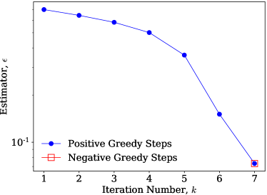
Figure 3: Convergence of greedy process for GMVR toy problem.

III.2 Modeling QNM frequencies with GMVP

In seeking to apply GMVP to select QNM frequencies, we wish to account for the known extremal Kerr behavior of some modes. Namely, we will impose a zero-damping constraint: some frequencies are real as $j_{f}\rightarrow 1$ Zimmerman & Mark (2016). We also wish to impose a domain transformation, $\kappa(j_{f},\ell,m)$, such that $0\leq\kappa\leq 1$ and the individual QNM frequencies are made approx. polynomial in $\kappa$.

For the domain transformation, inspection of QNM frequencies with $\ell\leq 5$ suggest that

$$\kappa(j_{f},\ell,m)=\left(\log_{3}(2-j_{f})\right)^{1/(2+\ell-|m|)}$$ (23)

appropriately linearizes the sharp behavior of each frequency near $j_{f}=1$ while also mapping $-1\leq j_{f}\leq 1$ onto $0\leq\kappa\leq 1$.

Towards the zero-damping constraint, when considering a QNM frequency $\tilde{\omega}_{{}_{\ell mn}}$, zero-damping at $j_{f}=1$ implies that $\tilde{\omega}_{{}_{\ell mn}}(\kappa\approx 0)-m/2\propto\kappa$, where $m/2$ is the well known limiting value for each QNM frequencies real part as $j_{f}\rightarrow 1$. This implies that

$$\tilde{\omega}_{{}_{\ell mn}}=m/2+\kappa\sum_{j=1}^{J}c_{j}\kappa^{k}\;.$$ (24)

In the case of the non-zero damped QNMs, (e.g. $(\ell,m)=(3,2)$), a more general polynomial form may be adopted, namely,

$$\tilde{\omega}_{{}_{\ell mn}}=\sum_{j=0}^{J}c_{j}\kappa^{k}\;.$$ (25)

The polynomial content of Eqn. (24) and Eqn. (25) is determined by GMVP. Equations (26)–(34) display the resulting polynomial models. In particular, the domain map allows most QNM frequencies to be well modeled by 4th order polynomials which include all lower degree terms; concurrently, the real and imaginary parts of each $\tilde{\omega}_{\ell mn}$ are modeled simultaneously.

Fig. 1 displays select training points, as well as model fits for $\tilde{\omega}_{\ell mn}$’s real and imaginary parts. For the top right and top left panels, the simple polynomial behavior of each curve is a result of the displayed linear domain in $\kappa(j_{f},\ell,m)$. In the top left panel, we have scaled $1/\tau_{\ell mn}$ by factors for $m/(n+1/2)$ to place the QNMs with $n=0$ and $n=1$ at approximately the same scale.

$$\tilde{\omega}_{220}(\kappa)\; =\;\,1.0\,+\,\kappa\,(1.5578e^{2.9031i}\,+\,1.9510e^{5.9210i}\kappa\,+\,2.0997e^{2.7606i}\kappa^{2}\,+\,1.4109e^{5.9143i}\kappa^{3}\,+\,0.4106e^{2.7952i}\kappa^{4}\,)$$ (26)

$$\tilde{\omega}_{221}(\kappa)\; =\;\,1.0\,+\,\kappa\,(1.8709e^{2.5112i}\,+\,2.7192e^{5.4250i}\kappa\,+\,3.0565e^{2.2857i}\kappa^{2}\,+\,2.0531e^{5.4862i}\kappa^{3}\,+\,0.5955e^{2.4225i}\kappa^{4}\,)$$ (27)

$$\tilde{\omega}_{330}(\kappa)\; =\;\,1.5\,+\,\kappa\,(2.0957e^{2.9650i}\,+\,2.4696e^{5.9967i}\kappa\,+\,2.6655e^{2.8176i}\kappa^{2}\,+\,1.7584e^{5.9327i}\kappa^{3}\,+\,0.4991e^{2.7817i}\kappa^{4}\,)$$ (28)

$$\tilde{\omega}_{331}(\kappa)\; =\;\,1.5\,+\,\kappa\,(2.3391e^{2.6497i}\,+\,3.1399e^{5.5525i}\kappa\,+\,3.5916e^{2.3472i}\kappa^{2}\,+\,2.4490e^{5.4435i}\kappa^{3}\,+\,0.7004e^{2.2830i}\kappa^{4}\,)$$ (29)

$$\tilde{\omega}_{440}(\kappa)\; =\;\,2.0\,+\,\kappa\,(2.6589e^{3.0028i}\,+\,2.9783e^{6.0510i}\kappa\,+\,3.2184e^{2.8775i}\kappa^{2}\,+\,2.1276e^{5.9897i}\kappa^{3}\,+\,0.6034e^{2.8300i}\kappa^{4}\,)$$ (30)

$$\tilde{\omega}_{430}(\kappa)\; =\;\,1.5\,+\,\kappa\,(0.2050e^{0.5953i}\,+\,3.1033e^{3.0162i}\kappa\,+\,4.2361e^{6.0388i}\kappa^{2}\,+\,3.0289e^{2.8262i}\kappa^{3}\,+\,0.9084e^{5.9152i}\kappa^{4}\,)$$ (31)

$$\tilde{\omega}_{550}(\kappa)\; =\;\,2.5\,+\,\kappa\,(3.2405e^{3.0279i}\,+\,3.4906e^{6.0888i}\kappa\,+\,3.7470e^{2.9212i}\kappa^{2}\,+\,2.4725e^{6.0365i}\kappa^{3}\,+\,0.6994e^{2.8766i}\kappa^{4}\,)$$ (32)

$$\tilde{\omega}_{320}(\kappa)\; =\;\,1.0225e^{0.0049i}\,+\,0.2473e^{0.6653i}\kappa\,+\,1.7047e^{3.1383i}\kappa^{2}\,+\,0.9460e^{0.1632i}\kappa^{3}\,+\,1.5319e^{5.7036i}\kappa^{4}$$ (33)

$$\hskip 255.0pt\,+\,2.2805e^{2.6852i}\kappa^{5}\,+\,0.9215e^{5.8417i}\kappa^{6}$$

$$\tilde{\omega}_{210}(\kappa)\; =\;\,0.5891e^{0.0435i}\,+\,0.1890e^{2.2899i}\kappa\,+\,1.1501e^{5.8101i}\kappa^{2}\,+\,6.0459e^{2.7420i}\kappa^{3}\,+\,11.1263e^{5.8441i}\kappa^{4}$$ (34)

$$\hskip 255.0pt\,+\,9.3471e^{2.6694i}\kappa^{5}\,+\,3.0384e^{5.7915i}\kappa^{6}$$

Fig. 1’s top left and right panels’ upper axes demonstrate the effect of mapping $j_{f}$ onto $\kappa$. In particular, it is shown that the two branches (namely $j_{f}>0$ and $j_{f}<0$) naturally form a single family of solutions when accounting for the sign of the BH’s oriented spin Husa et al. (2008). Concurrently, the use of $\kappa$ as a domain variable has the desirable effect of making each $\tilde{\omega}_{\ell mn}$ and $\tau_{\ell mn}$ approximately polynomial. We note that, in the asymptotic vicinity of $j_{f}=1$, the QNM frequencies and decay times are known to have solutions that are asymptoticly degenerate Zimmerman et al. (2015).

Algorithm 4 $\mathcal{A}_{\texttt{GMVR}}$, the action for GMVR. Model calculation given basis symbols, and output of model error estimate.

1:Input: { ${\bm{\lambda}}_{trial}$, $tol=10^{-3}$ }

2:Calculate $\alpha^{(1)}_{k}$ via Eqn. (19). Implicitly, $n=1$.

3:Calculate the current model prediction $g^{(1)}$ via Eqn. (20).

4:Calculate the model representation error, e.g.: $\epsilon^{(1)}=||var(g^{(n)}-g^{(0)})||/||g^{(0)}||$, where $var$ is the variance.

5:$done=False$

6:while  not $done$  do

7:    Calculate $\alpha^{n+1}_{k}$ via Eqn. (19).

8:    Calculate the current model prediction $g^{(n)}$ via Eqn. (20).

9:    Calculate the model representation error, e.g. $\epsilon^{(n)}=||g^{(n)}-g^{(0)}||/||g^{(0)}||$.

10:    $done=|\epsilon^{(n-1)}-\epsilon^{(n)}|<tol$

11:    (Implicitly, $n=n+1$)

12:end while

13:Output: $\epsilon^{(n)}$

In allowing Equations (26)–(34) to extrapolate to $j_{f}=1$, we do not explicitly account for this additional effect.

Fig. 1’s bottom two panels show absolute fractional residual errors of the complex frequency, $\tilde{\omega}_{\ell mn}=\omega_{\ell mn}+i/\tau_{\ell mn}$. Although each model’s fractional error is within 1% of the perturbation theory result, each is dominated by systematic error due to the choice fitting ansatz. For comparison, the same residual errors are shown in gray for the model presented in Ref. Berti et al. (2006); here, the sharp feature near $j_{f}=0$ results from their modeling counter and co-rotating QNM as two different curves.

Together, Equations (26)–(34) along with Fig. 1 present precise and accurate fits for the real and imaginary parts of QNM frequencies for gravitational perturbations of Kerr QNMs. A Python implementation of Equations (26)–(34) is available in Ref. London et al. (2018a) via positive.physics.cw181003550.

III.3 Modeling spherical-spheroidal inner-products with GMVR

Here we apply GMVR to the spherical-spheroidal mixing coefficients, $\sigma_{{}_{\bar{\ell}\bar{m}\ell mn}}$. As in the case of the QNM frequencies, we use the domain transformation defined by Eqn. (23) to simplify the functional form of each $\sigma_{{}_{\bar{\ell}\bar{m}\ell mn}}$.

While it is possible to enforce extremal Kerr and Schwarzschild limiting conditions for $\sigma_{{}_{\bar{\ell}\bar{m}\ell mn}}$, we find it effective to first use GMVR to determine a functional form that works for individual $\sigma_{{}_{\bar{\ell}\bar{m}\ell mn}}$, and then from these ansatz develop a single ansatz for all $\sigma_{{}_{\bar{\ell}\bar{m}\ell mn}}$. Equations (35)–(46) present the resulting model equations. A Python implementation of Equations (35)–(46) is available in Ref. London et al. (2018a) via positive.physics.ysprod181003550.

Fig. 4 displays fits, training data and related residuals. For efficiency of presentation, each $\sigma_{{}_{\bar{\ell}\bar{m}\ell mn}}$ is plotted via its real and imaginary part.

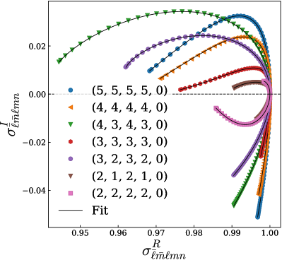
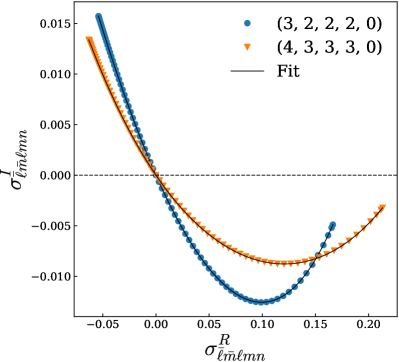
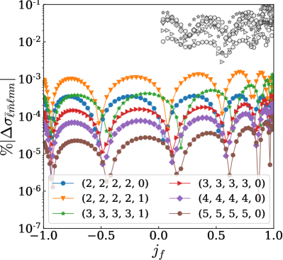
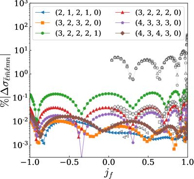
Figure 4: Spherical-spheroidal harmonic mixing coefficients and percentage residual errors for spherical-spheroidal harmonic mixing coefficient fits. (Top Left) Mixing coefficients for cases where $(\bar{\ell},\bar{m})=(\ell,m)$. The dashed horizontal intersects each curve at the Schwarzschild limit where $j_{f}=0$. (Top Right) Mixing coefficients where $(\bar{\ell},\bar{m})\neq(\ell,m)$. (Bottom Left and Right) Factional residuals for mixing coefficient fits. For comparison, residual errors for the fits in Ref. Berti & Klein (2014) are also shown over their region of validity in BH spin. Note that makers match between grey and colored data points.

In cases where $(\bar{\ell},\bar{m})=(\ell,m)$, the real part of $\sigma_{{}_{\bar{\ell}\bar{m}\ell mn}}$ varies about unity in a manner consistent with the Schwarzschild limit, where $\sigma_{{}_{\bar{\ell}\bar{m}\ell mn}}=\delta_{\bar{\ell}}^{\ell}\;\delta_{\bar{m}}^{m}$. Consistency with the Schwarzschild limit is equally true in cases where $(\bar{\ell},\bar{m})\neq(\ell,m)$. As with the QNM frequencies, residuals are dominated by small scale oscillations with amplitudes that are fractions of a percent of the central values, and largely result from the model asatz. For comparison, fractional residual errors for models in Ref. Berti & Klein (2014) are also shown.

IV Discussion

We have developed upon previous techniques for the linear and pseudo-linear modeling of low noise data. In particular, the GMVP algorithm performs multivariate polynomial modeling of real and complex valued scalar functions with no inherent limitation on the number of domain parameters. The GMVR algorithm does the same with multivariate rational functions. When applied to the modeling of analytically computed quantities, both algorithms perform extremely well in producing accurate and precise representations of training data, suggesting extended applicability of GMVR and GMVP to similar problems.

Treating a toy problem with GMVR demonstrates its ability to faithfully recover underlying model parameters for a plausible dataset. This treatment also demonstrates the convergence of the algorithm’s greedy phase with increasing iterations, as well as the convergence of an underlying iterative refinement phase (Eqn. 20).

Both GMVP and GMVR may be used to automatically determine the functional form and model for a given dataset that is expected to be respectively polynomial or rational. An alternative use-strategy is to use either GMVP or GMVR to determine a fitting ansatz for individual cases (e.g. individual QNMs), and then use these results to develop a single ansatz for all cases. This is what as been done for the modeling of QNM frequencies and spherical-spheroidal mixing coefficients.

GMVP has been applied to the modeling of QNM frequencies. The resulting models have been constrained in the extremal Kerr limit, and perform well compared to similar fits in the literature. The fits presented here are of direct use in Ref. London et al. (2018b), where efficiently evaluable QNM frequencies are required to generate template waveforms for GW searches and parameter estimation. The fits presented may find future use in Phenom or EOB based GW models.

GMVR has been applied to the modeling of mixing coefficients between the spherical and spheroidal harmonics.

Algorithm 5 GMVR, a degree tempered stepwise algorithm for multivariate rational modeling of scalar data.

1:Input: $\{x,f,$max_degree = 6$,tol\}$

2:Define, ${\bm{\lambda}}_{bulk}$, the bulk symbol space, to be the set of all multinomial combinations of basis vectors up to a predefined maximum order. This is the combined symbol space for numerator and denominator symbols.

3:Define $\mathcal{A}_{\texttt{GMVR}{}}$ according to Alg. (4).

4:Given $max\_degree$, define, ${D}$, a list of allowed polynomial degrees (e.g. $\{0,1,2,3,4,5,6\}$)

5:for $d$ in ${D}$  do

6:    Define ${\bm{\lambda}}_{bulk}^{(d)}$ as all symbols from ${\bm{\lambda}}_{bulk}$ with degree less than or equal to current degree: ${\bm{\lambda}}^{(d)}_{bulk}$

7:    Using ${\bm{\lambda}}_{bulk}^{(d)}$, apply Alg. (1), PGREEDY, with $\mathcal{A}_{\texttt{GMVP}{}}$ to get symbol subset, ${\bm{\lambda}}^{(d)}_{opt}$ and estimator val, $\epsilon^{(d)}_{opt}$

8:    if  $|\epsilon^{(d)}_{opt}-\epsilon^{(d-1)}_{opt}|<tol$  then

9:       break

10:    end if

11:end for

12:Output: ${\bm{\lambda}}^{(d)}_{opt}$

These fits are of direct use in Ref. Carullo et al. (2018), and may be of future use in similar ringdown-only models for the purpose of testing General Relativity.

While GMVR and GMVP show promise in the cases shown here, in their presented rudimentary form, both posses a number of limitations. If given sufficiently dense training data, neither currently performs cross-validation. And perhaps most notably, neither method directly accounts for information about the noise distribution within the training data. As such, the methods presented are recommended primarily for datasets where noise is very small or negligible. Nevertheless, the GMVR toy problem demonstrates GMVR’s ability to handle moderately noisy training data, suggesting current applicability to a variety of problems where polynomial interpolation is insufficient.

Of relevance to current and future GW science, the models presented for QNM frequencies and harmonic mixing coefficients have aided (e.g. Refs. Carullo et al. (2018); London (2018); London et al. (2018b) ), and are expected to continue aiding the development and implementation of GW signal models.

Appendix A Additional Equations

$$\sigma_{22220}\, =\,0.99733\,e^{6.2813i}\,+0.0075336\,\frac{14.592\,e^{5.0601i}\,\kappa\,+\,(28.761\,e^{1.629i})\,{\kappa}^{2}\,+\,(14.511\,e^{4.6362i})\,{\kappa}^{3}\,+\,(1.9624\,e^{3.0113i})}{1\,+\,0.88674\,e^{3.0787i}\,\kappa\,+\,(1.002\,e^{0.13211i})\,{\kappa}^{2}\,+\,(0.082148\,e^{5.6369i})\,{\kappa}^{3}}$$ (35)

$$\sigma_{21210}\, =\,0.99716\,e^{6.2815i}\,+0.0063542\,\frac{1.4345\times 10^{5}\,e^{4.5061i}\,\kappa\,+\,(3.5469\times 10^{5}\,e^{1.7327i})\,{\kappa}^{2}\,+\,(2.4038\times 10^{5}\,e^{5.1629i})\,{\kappa}^{3}\,+\,(6026.9\,e^{1.8881i})}{1\,+\,73780\,e^{4.5545i}\,\kappa\,+\,(97494\,e^{1.398i})\,{\kappa}^{2}\,+\,(34815\,e^{4.5623i})\,{\kappa}^{3}}$$ (36)

$$\sigma_{22221}\, =\,0.99683\,e^{6.2782i}\,+0.020758\,\frac{15.077\,e^{4.8323i}\,\kappa\,+\,(31.139\,e^{1.585i})\,{\kappa}^{2}\,+\,(15.449\,e^{4.6727i})\,{\kappa}^{3}\,+\,(0.71897\,e^{2.8084i})}{1\,+\,0.80592\,e^{3.3995i}\,\kappa\,+\,(0.69502\,e^{0.54275i})\,{\kappa}^{2}\,+\,(0.35613\,e^{5.9545i})\,{\kappa}^{3}}$$ (37)

$$\sigma_{32320}\, =\,0.99009\,e^{6.2804i}\,+0.02369\,\frac{71893\,e^{1.2395i}\,\kappa\,+\,(1.7055\times 10^{5}\,e^{5.0371i})\,{\kappa}^{2}\,+\,(1.2947\times 10^{5}\,e^{2.359i})\,{\kappa}^{3}\,+\,(1935.5\,e^{4.668i})}{1\,+\,38206\,e^{1.2254i}\,\kappa\,+\,(35811\,e^{3.9618i})\,{\kappa}^{2}\,+\,(8378.3\,e^{0.11726i})\,{\kappa}^{3}}$$ (38)

$$\sigma_{33331}\, =\,0.99478\,e^{6.2688i}\,+0.040478\,\frac{4.4113\,e^{1.2501i}\,\kappa\,+\,(11.588\,e^{0.27959i})\,{\kappa}^{2}\,+\,(17.322\,e^{3.7904i})\,{\kappa}^{3}\,+\,(0.67724\,e^{2.5797i})}{1\,+\,3.8782\,e^{2.2864i}\,\kappa\,+\,(3.4913\,e^{5.6655i})\,{\kappa}^{2}\,+\,(1.0368\,e^{2.9082i})\,{\kappa}^{3}}$$ (39)

$$\sigma_{32221}\, =\,0.02203\,e^{0.16452i}\,+0.073233\,\frac{24.932\,e^{1.0181i}\,\kappa\,+\,(30.197\,e^{4.4047i})\,{\kappa}^{2}\,+\,(11.274\,e^{2.981i})\,{\kappa}^{3}\,+\,(2.4374\,e^{6.1959i})}{1\,+\,11.397\,e^{3.9953i}\,\kappa\,+\,(10.915\,e^{5.8025i})\,{\kappa}^{2}\,+\,(7.2196\,e^{1.8176i})\,{\kappa}^{3}}$$ (40)

$$\sigma_{33330}\, =\,0.99569\,e^{6.2785i}\,+0.014546\,\frac{7.2112\,e^{0.62811i}\,\kappa\,+\,(6.5381\,e^{4.6216i})\,{\kappa}^{2}\,+\,(4.451\,e^{2.9228i})\,{\kappa}^{3}\,+\,(1.7113\,e^{2.9527i})}{1\,+\,1.4974\,e^{1.6687i}\,\kappa\,+\,(1.5288\,e^{5.3885i})\,{\kappa}^{2}\,+\,(0.52114\,e^{2.5471i})\,{\kappa}^{3}}$$ (41)

$$\sigma_{32220}\, =\,0.020598\,e^{0.04743i}\,+0.06919\,\frac{2.7657\,e^{2.133i}\,\kappa\,+\,(3.9562\,e^{4.653i})\,{\kappa}^{2}\,+\,(2.3364\,e^{2.6444i})\,{\kappa}^{3}\,+\,(2.399\,e^{6.2767i})}{1\,+\,1.0595\,e^{4.7865i}\,\kappa\,+\,(0.91308\,e^{2.887i})\,{\kappa}^{2}\,+\,(0.69468\,e^{0.1912i})\,{\kappa}^{3}}$$ (42)

$$\sigma_{43330}\, =\,0.028112\,e^{0.048488i}\,+0.086383\,\frac{12.087\,e^{0.47221i}\,\kappa\,+\,(30.626\,e^{3.3281i})\,{\kappa}^{2}\,+\,(16.328\,e^{6.1785i})\,{\kappa}^{3}\,+\,(2.3603\,e^{6.2662i})}{1\,+\,4.9638\,e^{3.5931i}\,\kappa\,+\,(6.2552\,e^{6.2001i})\,{\kappa}^{2}\,+\,(1.4538\,e^{2.5539i})\,{\kappa}^{3}}$$ (43)

$$\sigma_{43430}\, =\,0.98735\,e^{6.2795i}\,+0.033028\,\frac{7.0084\times 10^{5}\,e^{1.1067i}\,\kappa\,+\,(1.843\times 10^{6}\,e^{4.8808i})\,{\kappa}^{2}\,+\,(1.4367\times 10^{6}\,e^{2.1412i})\,{\kappa}^{3}\,+\,(13844\,e^{4.5601i})}{1\,+\,3.5667\times 10^{5}\,e^{1.0149i}\,\kappa\,+\,(3.274\times 10^{5}\,e^{3.7746i})\,{\kappa}^{2}\,+\,(88621\,e^{0.10095i})\,{\kappa}^{3}}$$ (44)

$$\sigma_{44440}\, =\,0.99478\,e^{6.2776i}\,+0.024791\,\frac{6.5172\,e^{0.79835i}\,\kappa\,+\,(7.7748\,e^{4.2485i})\,{\kappa}^{2}\,+\,(1.1577\,e^{1.5905i})\,{\kappa}^{3}\,+\,(1.2434\,e^{2.9616i})}{1\,+\,0.44548\,e^{1.2496i}\,\kappa\,+\,(0.59437\,e^{5.6732i})\,{\kappa}^{2}\,+\,(0.24743\,e^{2.8292i})\,{\kappa}^{3}}$$ (45)

$$\sigma_{55550}\, =\,0.99434\,e^{6.2773i}\,+0.03126\,\frac{6.5508\,e^{0.93398i}\,\kappa\,+\,(8.0558\,e^{4.2881i})\,{\kappa}^{2}\,+\,(0.92971\,e^{1.0436i})\,{\kappa}^{3}\,+\,(1.0904\,e^{2.9712i})}{1\,+\,0.23128\,e^{1.7666i}\,\kappa\,+\,(0.54958\,e^{5.9178i})\,{\kappa}^{2}\,+\,(0.213\,e^{3.0092i})\,{\kappa}^{3}}$$ (46)

References

- Abbott et al. (2016a) Abbott B. P., et al., 2016a, Phys. Rev., X6, 041015
- Abbott et al. (2016b) Abbott B. P., et al., 2016b, Phys. Rev. Lett., 116, 241102
- Abbott et al. (2016c) Abbott B. P., et al., 2016c, Astrophys. J., 833, L1
- Abbott et al. (2017) Abbott B. P., et al., 2017, Class. Quant. Grav., 34, 104002
- Berti & Klein (2014) Berti E., Klein A., 2014, Phys. Rev., D90, 064012
- Berti et al. (2006) Berti E., Cardoso V., Will C. M., 2006, Phys. Rev., D73, 064030
- Blackman et al. (2017) Blackman J., Field S. E., Scheel M. A., Galley C. R., Hemberger D. A., Schmidt P., Smith R., 2017, Phys. Rev., D95, 104023
- Bohé et al. (2017) Bohé A., et al., 2017, Phys. Rev., D95, 044028
- Buonanno & Damour (2000) Buonanno A., Damour T., 2000, Phys. Rev., D62, 064015
- Carullo et al. (2018) Carullo G., et al., 2018, arXiv:1805.04760.
- Caudill et al. (2012) Caudill S., Field S. E., Galley C. R., Herrmann F., Tiglio M., 2012, Class.Quant.Grav., 29, 095016
- Cotesta et al. (2018) Cotesta R., Buonanno A., Bohé A., Taracchini A., Hinder I., Ossokine S., 2018
- Epperson (1987) Epperson J. F., 1987, The American Mathematical Monthly, 94, 329
- Field et al. (2011) Field S. E., Galley C. R., Herrmann F., Hesthaven J. S., Ochsner E., Tiglio M., 2011, Phys. Rev. Lett., 106, 221102
- Hannam et al. (2014) Hannam M., Schmidt P., Bohé A., Haegel L., Husa S., Ohme F., Pratten G., Pürrer M., 2014, Phys. Rev. Lett., 113, 151101
- Husa et al. (2008) Husa S., González J. A., Hannam M., Brügmann B., Sperhake U., 2008, Class. Quant. Grav., 25, 105006
- Khan et al. (2016) Khan S., Husa S., Hannam M., Ohme F., Pürrer M., Jiménez Forteza X., Bohé A., 2016, Phys. Rev., D93, 044007
- Leaver (1985) Leaver E., 1985, Proc.Roy.Soc.Lond., A402, 285
- London (2018) London L., 2018, arXiv:1801.08208.
- London et al. (2014) London L., Shoemaker D., Healy J., 2014, Phys. Rev., D90, 124032
- London et al. (2018a) London L., Fauchon-Jones E., EZHamilton 2018a, llondon6/positive: charge, doi:10.5281/zenodo.1402516, https://doi.org/10.5281/zenodo.1402516
- London et al. (2018b) London L., et al., 2018b, Phys. Rev. Lett., 120, 161102
- Moore (1920) Moore E. H., 1920, Bulletin of the American Mathematical Society, 26, 394
- Nagar et al. (2018) Nagar A., et al., 2018
- Pan et al. (2014) Pan Y., Buonanno A., Taracchini A., Kidder L. E., Mroué A. H., Pfeiffer H. P., Scheel M. A., Szilágyi B., 2014, Phys. Rev., D89, 084006
- Penrose (1955) Penrose R., 1955, Mathematical Proceedings of the Cambridge Philosophical Society, 51, 406
- Press et al. (1992) Press W. H., Teukolsky S. A., Vetterling W. T., Flannery B. P., 1992, Numerical Recipes in C: The Art of Scientific Computing, second edn. Cambridge University Press, pp 204–208
- Schmidt et al. (2015) Schmidt P., Ohme F., Hannam M., 2015, Phys. Rev., D91, 024043
- Teukolsky (1972) Teukolsky S. A., 1972, Phys. Rev. Lett., 29, 1114
- Yang et al. (2013) Yang H., Zhang F., Zimmerman A., Nichols D. A., Berti E., Chen Y., 2013, Phys. Rev., D87, 041502
- Zimmerman & Mark (2016) Zimmerman A., Mark Z., 2016, Phys. Rev., D93, 044033
- Zimmerman et al. (2015) Zimmerman A., Yang H., Zhang F., Nichols D. A., Berti E., Chen Y., 2015