Scaling laws in the stellar mass distribution and the transition to homogeneity

Abstract

We present a new statistical analysis of the large-scale stellar mass distribution in the Sloan Digital Sky Survey (data release 7). A set of volume-limited samples shows that the stellar mass of galaxies is concentrated in a range of galaxy luminosities that is very different from the range selected by the usual analysis of galaxy positions. Nevertheless, the two-point correlation function is a power-law with the usual exponent $\gamma=1.71$–$1.82$, which varies with luminosity. The mass concentration property allows us to make a meaningful analysis of the angular distribution of the full flux-limited sample. With this analysis, after suppressing the shot noise, we extend further the scaling range and thus obtain $\gamma=1.83$ and a clustering length $r_{0}=5.8$–$7.0\,h^{-1}$Mpc. Fractional statistical moments of the coarse-grained stellar mass density exhibit multifractal scaling. Our results support a multifractal model with a transition to homogeneity at about $10\,h^{-1}$Mpc.

1 Introduction

It is claimed that we are entering the era of precision cosmology, in which the fundamental parameters of the universe are known within a few percent precision and only remains to progressively refine them (Jones, 2017; Lahav and Liddle, 2017). In addition to the global parameters of the FLRW model, we have the parameters that determine the primordial density perturbations and hence the formation of large scale structure. A particularly interesting parameter is the amplitude of the primordial density perturbations, usually measured in terms of the present linear-theory mass dispersion on a scale of 8 $h^{-1}$Mpc, named $\sigma_{8}$. The scale of 8 $h^{-1}$Mpc comes from Peebles’ observation that galaxy counts on this scale have a rms fluctuation approximately equal to one (Peebles, 1993). In general, the mass dispersion over the length $R$, $\sigma(R)$, defines a scale such that $\sigma(R)=1$. This scale separates the linear and quasi-homogeneous regime of the evolution of density fluctuations from the nonlinear regime of strong clustering.

A similar scale is the distance $r_{0}$ such that $\xi(r_{0})=1$, where $\xi(r)$ is the reduced galaxy-galaxy correlation function. Actually, this function is well approximated by the power law

$$\xi(r)=\left(\frac{r_{0}}{r}\right)^{\gamma},$$ (1)

for distances not much larger than $r_{0}$ (Peebles, 1993). The scale such that the rms dispersion of galaxy counts is equal to one is related to $r_{0}$ by a $\gamma$-dependent factor (Peebles, 1993). Historically, the power-law form of $\xi(r)$ was deduced from the angular positions of galaxies, yielding $\gamma=1.8$ and $r_{0}=4.7\,h^{-1}$Mpc (Totsuji and Kihara, 1969; Groth and Peebles, 1977). Nowadays, good galaxy redshift surveys are available, but the angular positions are still useful. In particular, the angular correlation function $w(\theta)$ is used, in combination with other data, to determine precision values of $\sigma_{8}$ (Lahav and Liddle, 2017; DES Collaboration, 2018).

The amplitude of the primordial density perturbations is not theoretically constrained and determines the present scale of transition to homogeneity, which can have any value, once given the global cosmological parameters. The transition to homogeneity has been the subject of numerous studies, some of them motivated by the bold proposal that the scale of homogeneity is too large to be accessible or even that no such transition exists (Mandelbrot, 1983; Pietronero, 1987; Coleman and Pietronero, 1992). This proposal, namely, that the mass distribution is fully scale invariant, at all scales in a Newtonian cosmology, has been called the “fractal universe” (Peebles, 1993). Actually, Eq. (1) corresponds to a fractal distribution on scales $r\ll r_{0}$, for any magnitude of $r_{0}$.

The scale and specific form of transition to homogeneity determine the size of the largest structures, although these structures can have a length much larger than $r_{0}$ (Gaite, Domínguez and Pérez-Mercader, 1999). An examination of the literature shows values of the scale of transition to homogeneity that go from the standard value of 5 $h^{-1}$Mpc (Peebles, 1993) to more than 20 $h^{-1}$Mpc (Sylos Labini, Vasilyev and Baryshev, 2007; Sarkar et al., 2009; Verevkin, Bukhmastova and Baryshev, 2011; Chacón-Cardona et al., 2016). The range that these values span is quite long. In contrast, the current precision values of $\sigma_{8}$ are assigned a relative error of about one percent (Lahav and Liddle, 2017). This precision is surprisingly good, in comparison, given that $\sigma_{8}$ determines the scale of transition to homogeneity.

Most of the literature about the large-scale structure of the universe based on the statistical analysis of galaxy catalogs is limited to the distribution of the galaxy positions. We make here, following up on Gaite (2018), a new statistical analysis of the large-scale structure, adding an important ingredient: the stellar masses of galaxies; that is to say, we study the large-scale distribution of stellar mass. The distribution of stellar mass in the SDSS has already been studied by Li and White (2009), employing the projected correlation function $w(r_{\mathrm{p}})$, on scales $r_{\mathrm{p}}<30\,h^{-1}$Mpc [$r_{\mathrm{p}}$ is the separation perpendicular to the line of sight (Davis and Peebles, 1983)]. Li and White find that $w(r_{\mathrm{p}})$ is very well represented, over the range $10\,h^{-1}$kpc $<r_{\mathrm{p}}<$ $10\,h^{-1}$Mpc, by a power law that corresponds to Eq. (1) with $\gamma=1.84$ and $r_{0}=6.1\,h^{-1}$Mpc. These results basically agree with the analysis of the SDSS galaxy positions by Zehavi et al. (2011), but Li and White deem the scaling of the stellar mass to be better. At any rate, the stellar mass and galaxy number distributions can be shown to be very different, thus warranting further statistical analysis.

Besides, we must take into account that the “projection” that produces $w(r_{\mathrm{p}})$ is performed on the correlation function $\xi(r)$ and is not associated to an actual projected distribution but to a set of local orthogonal projections on the tangent planes to the surface of the unit sphere (a rather unwieldy construction from the mathematical standpoint). Arguably, the direct study of the angular projection of the stellar mass distribution is preferable. On the other hand, there are statistical measures not based on the two-point correlation function. Our study combines the analysis of a set of volume-limited samples with an angular analysis and, moreover, involves various statistical measures.

The importance of galaxy masses in the study of galaxy clustering was recognized years ago (Pietronero, 1987). Furthermore, Pietronero (1987) argued that a full multifractal analysis of galaxy clustering is necessary. A multifractal model was also proposed by Jones et al. (1988), without considering the galaxy masses. Pietronero and collaborators initiated the multifractal analysis with masses of galaxies derived from the observed luminosities by assuming a simple mass-luminosity relation (Coleman and Pietronero, 1992; Sylos Labini, Montuori and Pietronero, 1998). Meanwhile, the large-scale structure has been known to consist not just of clusters but of a web structure (Geller and Huchra, 1989; Kofman et al., 1992). This structure can be described as a multifractal (Gaite, 2018, 2019). Multifractality has become essential to the scaling analysis of the distribution of galaxies, although normally without considering the galaxy masses (Borgani, 1995; Jones et al., 2004).

As we shall see, most of a multifractal structure is preserved in an angular projection. Pietronero (1987) already considered some basic properties of the angular projection of a fractal galaxy distribution. This question was further studied by Coleman and Pietronero (1992) and Durrer et al. (1997), assuming a monofractal model.

Our galaxy data come from the Sloan Digital Sky Survey, data release 7 (SDSS DR7) (Abazajian et al., 2009), as provided by the New York University Value-Added Galaxy Catalog (NYU-VAGC) (Blanton et al., 2005). The NYU-VAGC contains the stellar masses of the galaxies, calculated with the method described by Blanton and Roweis (2007) (which gives similar results to the method of Kauffmann et al. 2003). In fact, we use the same data as Li and White (2009), which facilitates the comparison of the respective results. Moreover, the SDSS DR7 is well studied and, in particular, there is a careful analysis of its galaxy-galaxy angular correlation function (Wang, Brunner and Dolence, 2013). We have already employed the same data to make a multifractal analysis of the stellar mass distribution based on the convergence of multifractal spectra for a shrinking scale (Gaite, 2018). The present treatment of scaling laws is much more elaborate, allowing us to compare with the preceding studies of scaling in the SDSS and to study the transition to homogeneity.

Our plan is as follows. We begin in Sect. 2 with a short discussion of scaling, fractality and homogeneity in galaxy surveys and of the role played by the scale-dependent mass variance. In Sect. 3, we apply these concepts to the study of a set of volume-limited samples from the SDSS DR7 and to the analysis of scaling of the respective mass variances. Multifractality is proved by the analysis of fractional statistical moments in Sect. 4. We next consider the theory of projection of fractal distributions in Sect. 5, and we connect this theory with the standard theory of the angular two-point correlation function of galaxies (Sect. 5.1). After this theoretical study, we undertake the analysis of the angular projection of the SDSS DR7 in Sect. 6, where we deal with the increased shot noise (Sect. 6.1) and we obtain $r_{0}$ from the variance of the coarse-grained angular density (Sect. 6.2). We end with a general discussion (Sect. 7).

2 Scaling, fractality and homogeneity in galaxy surveys

It is pertinent to begin with some general considerations about scaling and homogeneity in galaxy surveys, and, in particular, about how to characterize fractality and how to determine the scale of transition to homogeneity. Let us assume that we can obtain the three-dimensional stellar mass distribution, which requires a redshift survey with galaxy stellar masses and the construction of volume limited samples.

Taking the two-point correlation function as the basic statistic, the fundamental scaling law is the power-law reduced correlation function in Eq. (1). This law is supposed to hold when $\xi(r)$ is not small, that is to say, for $r$ not much larger than $r_{0}$ (but it could also be valid for $r\gg r_{0}$). The coarse-grained mass fluctuation $\delta M_{R}/M_{R}$, namely, the scale dependent rms fluctuation of the stellar mass in a cell of linear dimension $R$, derives from the reduced two-point correlation function of the mass distribution. If this function follows the power law (1), the mass variance follows a power law with the same exponent, namely,

$$\left(\frac{\delta M_{R}}{M_{R}}\right)^{2}=C(\gamma)\left(\frac{r_{0}}{R}\right)^{\gamma},$$ (2)

where the form of $C(\gamma)$ depends on the shape of the cell (Peebles, 1993).

Regardless of any scaling property, $\delta M_{R}/M_{R}$ must decrease with $R$ and the scale of homogeneity can be defined just by the condition $\delta M_{R}/M_{R}=1$. However, this is too stringent a criterion for homogeneity. Indeed, let us notice that a positive random variable with a rms dispersion equal to its mean value cannot be approximately Gaussian; for example, let us consider the lognormal distribution (see Coles and Jones, 1992, p. 5). A suitable criterion for homogeneity is the mass variance $(\delta M_{R}/M_{R})^{2}=0.1$, as assumed by Gaite (2018); indeed, a lognormal distribution function with this variance is hardly skewed (Coles and Jones, 1992, p. 5). Whether or not the scale defined by $(\delta M_{R}/M_{R})^{2}=0.1$ is close to the one defined by $\delta M_{R}/M_{R}=1$ depends on how sharp the transition to homogeneity is. To analyze this question, we naturally choose the power law form in Eq. (2).

For a spherical cell of radius $R$, $C(\gamma)$ in Eq. (2) is given by Peebles (1993). The scale $R$ such that $\delta M_{R}/M_{R}$ equals a given number is a definite function of $\gamma$. For $\delta M_{R}/M_{R}=1$, $R$ is only a little larger than $r_{0}$, whereas, for $(\delta M_{R}/M_{R})^{2}=0.1$, it is between $4.7r_{0}$ and $12r_{0}$ (the larger, the smaller $\gamma$ is). In conclusion, the scale such that $\delta M_{R}/M_{R}=1$ is roughly equivalent to $r_{0}$ but the scale where the probability distribution is approximately Gaussian can be several times larger. This observation reveals that the values $r_{0}=5.4\,h^{-1}$Mpc and $\gamma=1.8$ are compatible with the presence of relatively large structures, for example, cosmic voids of size $\simeq 30\,h^{-1}$Mpc (Peebles, 1993). Actually, even larger structures can be observed, provided that $\xi(r)$ does not fall too rapidly for $r\gg r_{0}$ (Gaite, Domínguez and Pérez-Mercader, 1999).

After clarifying our concept of homogeneity, let us now recall several aspects of scale invariance and fractal geometry. First of all, let us remark that the fractal geometry of a mass distribution consists in some sort of scale invariance in the strongly inhomogeneous or strong clustering regime. Its most general form is called multifractality and is expressed in terms of the multifractal spectrum $f(\alpha)$ or, alternatively, of the Rényi dimension spectrum $D_{q}$ (Harte, 2001; Falconer, 2003). The multifractal spectrum $f(\alpha)$ is a basic function that represents how mass concentrates, in terms of the number of mass concentrations of a given “strength”, measured by the local dimension $\alpha$, while the Rényi dimensions provide a sort of averaged information. The functions $f(\alpha)$ and $D_{q}$ are related by a Legendre transform in terms of the variables $\alpha$ and $q$. The Rényi dimension $D_{q}$ expresses the scaling of the statistical $q$-moment of the coarse-grained mass distribution and is, in general, a non-increasing function of $q$. The second order moment has an intuitive meaning and the corresponding Rényi dimension is $D_{2}=3-\gamma$. General $q$-moments and their scaling relations are studied in Sect. 4.

It is to be remarked that the primary concept of fractal dimension and its various definitions are concerned with the small scale behavior of sets or mass distributions, and fractality is roughly equivalent to asymptotic scaling in the limit of vanishing scale, as described in standard fractal geometry textbooks (Harte, 2001; Falconer, 2003). In consequence, multifractal measures are defined for any mass distribution, regardless of its behavior on large scales. An arbitrary mass distribution is not expected to be such that it becomes homogeneous on large scales, tending to a uniformly homogeneous state, as occurs in cosmology because of the cosmological principle. This is why raw statistical $q$-moments $\langle M^{q}\rangle$ are employed in fractal geometry, instead of central moments, which require a globally defined mean density.

To make the cosmological principle compatible with fractal models of strong clustering, Mandelbrot (1983) proposed the conditional cosmological principle, in which “every possible observer” is replaced with “every observer located at a material point”. Thus, the natural measure for the fractal analysis of strong clustering is the conditional density, namely, the average density at a distance $r$ from an occupied point (Mandelbrot, 1983; Coleman and Pietronero, 1992; Sylos Labini, Montuori and Pietronero, 1998). It can be expressed as

$$\Gamma(r)=\frac{\langle\varrho(\bm{r})\,\varrho(\bm{0})\rangle}{\langle\varrho\rangle}=\langle\varrho\rangle\left(\xi(r)+1\right).$$ (3)

But it is conceptually independent of the mean density $\langle\varrho\rangle$, is spite of the fact that it appears in these expressions.

Motivated by these ideas, some authors look for scaling of the conditional density $\Gamma(r)$ of the galaxy distribution (or of its integral in the ball of radius $r$). When calculated with this method, the scale of homogeneity is often large (Sylos Labini, Vasilyev and Baryshev, 2007; Verevkin, Bukhmastova and Baryshev, 2011). The conditional density is not used by traditional cosmologists, who are accustomed to the function $\xi(r)$. If $\langle\varrho\rangle\neq 0$, then the conditional density $\Gamma(r)$ is conceptually useful but can be expressed in terms of $\xi(r)$, by Eq. (3), and it scales as $\xi(r)+1$. Naturally, the condition for fractal scaling is $\xi\gg 1$, which makes $\xi$ and $\xi+1$ equivalent. However, the condition is never fulfilled in a sufficiently long range of $r$. Therefore, the values of $r_{0}$ and $\gamma$ obtained from power-law fits of either function differ, namely, $r_{0}$ is larger when calculated from $\xi+1$. Let us illustrate this point with an example, employing a sample from Gaite (2018).

Gaite (2018) uses a method of multifractal analysis based on coarse-graining cells that are adapted to the SDSS sample geometry. These cells are not spherical nor have a simple shape, but have equal volume, which serves to measure their size. Let this volume be $v$. The second moment of the coarse-grained density is

$$\mu_{2}(v)=\frac{\langle\varrho_{v}^{2}\rangle}{\langle\varrho_{v}\rangle^{2}}\,,$$ (4)

and the density variance (mass variance) is

$$\mu_{2}(v)-1=\frac{\langle{\delta\varrho_{v}}^{2}\rangle}{\langle\varrho_{v}\rangle^{2}}=\frac{\langle{\delta M_{v}}^{2}\rangle}{\langle M_{v}\rangle^{2}}\,.$$ (5)

The scaling law (1) is equivalent to the scaling law for the mass variance (2). Likewise, a scaling law for $\xi(r)+1$ is equivalent to a scaling law for $\mu_{2}(v)$. An example of both the scaling laws for $\mu_{2}(v)$ and $\mu_{2}(v)-1$ is displayed in Fig. 1, which we now explain.

Fig. 1 refers to a volume limited sample of 1765 galaxies in the redshift range $(0.003,0.013)$, defined by Gaite (2018) and called VLS1. This sample was adequate to compute a quite complete multifractal spectrum and is now useful to test the two options for the scaling law that yields $D_{2}$. The solid blue lines in Fig. 1 are the graphs of $\mu_{2}$ and $\mu_{2}-1$. The fit to the power law

$$\mu_{2}=(v/v_{0})^{-\gamma/3}$$ (6)

in the interval $v\in[3,190]$ Mpc³/$h^{3}$ yields $v_{0}=(1960\pm 180)$ Mpc³/$h^{3}$ and $\gamma=1.57\pm 0.01$, that is to say, $D_{2}=3-\gamma=1.43\pm 0.01$ (the power-law fit is a least-squares linear fit of $\log\mu_{2}$ versus $\log v$). An analogous fit to the power law

$$\mu_{2}-1=(v/v_{0})^{-\gamma/3}$$ (7)

yields $v_{0}=(850\pm 300)$ Mpc³/$h^{3}$ and $D_{2}=1.20\pm 0.06$ ($\gamma=1.80\pm 0.06$). Both fits are represented by dashed red lines in Fig. 1. The latter fit, with $\gamma=1.80$ and $v_{0}^{1/3}=9.5$ Mpc/$h$, basically agrees with the canonical values of $\gamma$ and $r_{0}$ (from the reduced two-point correlation function of galaxy positions). However, both fits are questionable for calculating $D_{2}$, because the fractal regime demands $\mu_{2}-1\approx\mu_{2}\gg 1$, but the fitted range extends beyond the small scales where this condition holds. Therefore, some intermediate values of $v_{0}$ and $\gamma$ should be more appropriate. These values are uncertain because we have too small a range of scales with both $\mu_{2}\gg 1$ and negligible discreteness effects. These effects make $D_{2}$ shrink towards $D_{2}=0$, as the steeper left ends of the graphs reflect.

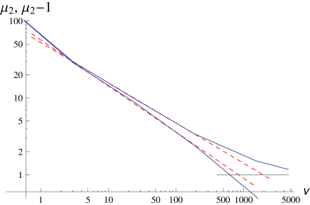
Figure 1: Fits to scaling for sample VLS1: moments $\mu_{2}(v)$ and $\mu_{2}(v)-1$ ($v$ in Mpc${}^{3}/h^{3}$), with fits to the scaling $(v/v_{0})^{-\gamma/3}$, represented as dashed lines. The crossing of each dashed line with the horizontal gray line gives $v_{0}$.

The uncertainties of 20% in $D_{2}$ and 30% in $v_{0}^{1/3}$ due to the limited scaling range can be compared with the uncertainties in galaxy positions and masses. Gaite (2018) has analyzed how these uncertainties affect the multifractal spectrum of VLS1, with the result that only the right-hand side part of the spectrum is affected (Gaite, 2018, left-hand side of Fig. 4). This implies that only the (Rényi) dimensions $D_{q}$ with $q<0$ are affected. Therefore, the evaluation of $D_{2}$ should not be affected. To confirm it, we calculate now the uncertainty of $\mu_{2}(v)$ due to the uncertainty of galaxy positions and masses. To do it, we employ the same procedure as Gaite (2018), namely, we generate ten variant samples, with values of redshift and stellar mass given by, respectively, Gaussian and lognormal distributions with variances in accord with the literature. The variant samples yield ten values of $\mu_{2}$ for each value of $v$, and we compute for each $v$ the standard deviation of those ten values. The result is that the relative error of $\mu_{2}$ is always smaller than 4.2% (the corresponding error bars in Fig. 1 would hardly be visible).

As regards errors in the linear fits, their magnitude grows as one tries to fit more points, and the natural criterion to stop is to minimize the rms error per degree of freedom (the number of degrees of freedom is the number of points minus two). In most of the fits here, these errors are quite small in comparison with errors from other sources. The relative small uncertainty due to statistical errors in galaxy positions and masses combined with the smallness of errors in the linear fits shows that the major uncertainty in the fractal analysis is due to discreteness effects, that is to say, to limitations imposed by a small fractal scaling range.

Gaite (2018) observes that the low-redshift VLS1 obtains a multifractal spectrum that is more complete than the ones obtained from higher-redshift volume-limited samples. We find that higher-$z$ samples are also less useful to directly calculate $D_{2}$ as above. The higher $z$ is in a volume-limited sample the more luminous the galaxies in it and the smaller their number density (as we shall discuss when we construct a set of volume-limited samples in Sect. 3). A smaller number density implies that discreteness effects take over growing ranges of the smaller scales, reducing the interval of scales where the fractal regime can be measured, that is to say, the interval where $\mu_{2}-1\approx\mu_{2}\gg 1$.

However, we may consider the scaling of just $\mu_{2}(v)-1$, in the longest possible interval, without demanding that $\mu_{2}(v)-1>1$. For example, one can dismiss the upper graph in Fig. 1, corresponding to $\mu_{2}$, and think of extending the scaling of $\mu_{2}-1$ below the line $\mu_{2}-1=1$. Likewise, Eq. (1) usually extends to $\xi<1$ (weak correlations). Besides, we remark that the frequently employed projected correlation function $w(r_{\mathrm{p}})$ (e.g., by Zehavi et al. 2011 or Li and White 2009) is a dimensional function that renders obscure the strength of correlations. The range with $\xi<1$ is the appropriate one for the molecular correlations in statistical physics, and scale invariance takes place in critical phenomena. In this regard, we can expect that Eq. (1) holds from the small scales where $\xi\gg 1$ to the large scales where $\xi\ll 1$, encompassing the fractal and critical-fluid regimes (Gaite, Domínguez and Pérez-Mercader, 1999).

At any rate, what we conclude from the analysis of VLS1 is that the statistical analysis of the stellar mass distribution in the SDSS-DR7 by means of volume-limited samples is plagued with errors, especially, discreteness errors. An alternative to it is the study of the projected angular distribution, which has two advantages. On the one hand, we avoid the influence of redshift space distortions on the statistics, which is considerable (Zehavi et al., 2011). On the other hand, we have all points in the angular region, whereas volume-limited samples span the same angular region but occupy very different three-dimensional regions (which are awkwardly shaped, in addition). We see next the information obtained from a systematic study of volume-limited samples and leave the study of the angular projection to Sect. 5.

3 Volume-limited samples

To be systematic in the study of the three-dimensional mass distribution, we construct volume-limited samples in successive intervals of absolute magnitude; for example, in the SDSS, one can take intervals in which it changes by one unit. We follow the procedure and conventions of Zehavi et al. (2011) (the absolute magnitude is denoted by $M_{\mathrm{r}}$, not to be confused with our notation of $M$ as a mass).

We employ the same SDSS-DR7 data from the NYU-VAGC as in Gaite (2018), and we also select the apparent magnitude range $12.5<m_{\mathrm{r}}<17.77$. The angular ranges are defined in terms of equal-area coordinates $sl=\sin\lambda$ and $f=\eta+0.567$ radians, where the angles $\lambda$ and $\eta$ constitute the SDSS coordinate system. The available ranges of our coordinates are $-0.760<sl<0.793$ and $-0.0227<f<1.200$ (radians), providing a total solid angle $\Omega=1.554\cdot 1.222=1.899$ steradians. We further restrict the sample to $z<0.34$, obtaining $529\hskip 1.0pt655$ galaxies.

$M_{\mathrm{r}}$	$z$	$N$	$n$	dens.	mass
$(-14,-15)$	0.0011–0.0073	554	0.08550	0.009	$(2.7~{}10^{4},1.4~{}10^{8})$
$(-15,-16)$	0.0017–0.0115	885	0.03472	0.010	$(4.1~{}10^{5},4.0~{}10^{8})$
$(-16,-17)$	0.0026–0.0181	1708	0.01717	0.012	$(9.4~{}10^{6},9.2~{}10^{8})$
$(-17,-18)$	0.0042–0.0284	6625	0.01728	0.039	$(1.7~{}10^{6},2.8~{}10^{9})$
$(-18,-19)$	0.0066–0.0444	17416	0.01202	0.089	$(1.2~{}10^{7},6.1~{}10^{9})$
$(-19,-20)$	0.0105–0.0689	46204	0.00870	0.203	$(2.1~{}10^{7},2.3~{}10^{10})$
$(-20,-21)$	0.0165–0.1058	97847	0.00522	0.333	$(1.7~{}10^{6},6.6~{}10^{10})$
$(-21,-22)$	0.0260–0.1613	101350	0.00159	0.247	$(1.2~{}10^{7},1.7~{}10^{11})$
$(-22,-23)$	0.0406–0.2444	30680	0.00015	0.056	$(7.5~{}10^{8},4.4~{}10^{11})$
$(-23,-24)$	0.0632–0.3597	1460	$2.4~{}10^{-6}$	0.002	$(7.7~{}10^{9},7.9~{}10^{11})$

Table 1: Characteristics of the volume-limited samples: absolute magnitude, redshift, number of galaxies, number density ($h^{3}$ Mpc^-3), fraction of the total mass density, and galaxy mass ($M_{\odot}$).

The main characteristics of our volume-limited samples are reported in Table 1. Naturally, the redshift intervals are almost coincident with the ones of Zehavi et al. (2011), but the the number of galaxies in each sample is larger, because the angular region is larger. The number of galaxies grows with absolute luminosity, up to $M_{\mathrm{r}}\in(-21,-22)$, with $N=101\hskip 1.0pt350$. This growth might suggest that discreteness effects are reduced up to this point, but the number density shrinks and the overall effect is that discreteness progressively hinders the detection of strong clustering, as noticed in Sect. 2. For instance, the sample with $M_{\mathrm{r}}\in(-21,-22)$ and number density $0.00159$ has a volume per galaxy of $629$ Mpc${}^{3}\!/h^{3}$, that is to say, the equivalent length is $8.6$ Mpc$/h$, as large as the expected value of $r_{0}$.

As regards number density, the best sample is the first one, with $M_{\mathrm{r}}\in(-14,-15)$ and number density $0.08550$ (this sample is somewhat like the VLS1 studied in Sect. 2). However, we are studying here the distribution of mass rather than the distribution of individual galaxies and the sample represents a fraction of the total mass density that only amounts to $0.009$. Thus, the clustering properties of the full mass distribution are hardly influenced by the galaxies with $M_{\mathrm{r}}\in(-14,-17)$, in spite of their abundance.

The last variable in Table 1 is the galaxy mass, and we can observe the evident correlation between galaxy mass and absolute luminosity. This correlation is significant in the multifractal analysis, because this analysis distinguishes the strength of mass concentrations, measured by the local dimension $\alpha$. To be precise, the concentration strength is measured in coarse multifractal analysis by the logarithm of the mass in each cell, namely, $\alpha=-\log m/\ln l$, (Falconer 2003, applied to cosmology by Gaite 2007). However, galaxies are not equal-size mass concentrations and, actually, the galaxy sizes are not even part of the data. Nevertheless, it is to be expected that the stellar mass in the more luminous samples is more concentrated. Therefore, we also expect that the set of values of $\alpha$ and hence the dimension $D_{q}$ of each sample are smaller the more luminous the galaxies in it.

3.1 Scaling of cell mass variances

Here we examine if cell mass variances are power-law functions of the cell volume $v$, according to Eq. (7) and employing the coarse-graining method of Gaite (2018) as in Sect. 2. We focus on the three galaxy samples in Table 1 in the interval $M_{\mathrm{r}}\in(-19,-22)$, whose contribution to the total mass density is dominant (more than 78%). But we also examine, to be thorough, the two adjacent samples, to include most of the total mass density as well as most galaxies in the set of samples.

$M_{\mathrm{r}}$	$\gamma$	$v_{0}^{1/3}$
$(-18,-19)$	$1.52\pm 0.07$	$13.5\pm 1.6$
$(-19,-20)$	$1.71\pm 0.04$	$12.4\pm 0.8$
$(-20,-21)$	$1.616\pm 0.013$	$14.2\pm 0.3$
$(-21,-22)$	$1.818\pm 0.007$	$16.9\pm 0.2$
$(-22,-23)$	$1.93\pm 0.02$	$29.4\pm 0.6$

Table 2: Results for scaling in the five volume-limited samples with higher mass density ($v_{0}^{1/3}$ in Mpc$/h$).

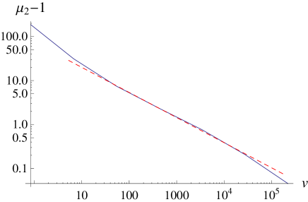
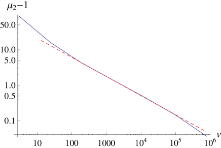
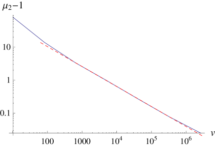
Figure 2: Variance $\mu_{2}(v)-1$ of the stellar mass distribution ($v$ in Mpc${}^{3}/h^{3}$), for three volume-limited samples: $M_{\mathrm{r}}\in(-19,-20)$ (upper plot), $M_{\mathrm{r}}\in(-20,-21)$ (middle plot), and $M_{\mathrm{r}}\in(-21,-22)$ (lower plot). The linear fits yield the values of $\gamma$ and $v_{0}^{1/3}$ in Table 2.

The results of the calculation and plotting of $\mu_{2}(v)-1$ appear in Table 2 and Fig. 2. To wit, in Fig. 2 are the log-log plots of $\mu_{2}(v)-1$ for the three samples with $M_{\mathrm{r}}\in(-19,-22)$, and in Table 2 are the numerical results of the log-log linear fits corresponding to the five volume-limited samples of Table 1 with higher mass density. We obtain a nontrivial scaling for intermediate values of $v$, which crosses over, for small $v$, to the trivial scaling corresponding to isolated points ($D_{2}=0$). It is remarkable that the scalings displayed in Fig. 2 hold in considerable ranges that go across the point of unit variance, extending from the moderately strong clustering regime to the quasi-homogeneous regime.

Regarding the values of the scaling exponent $\gamma$ in Table 2, we can observe a definite growing trend, except in the sample with $M_{\mathrm{r}}\in(-20,-21)$ (an anomaly in this range is also noted by Zehavi et al. 2011). The length scale $v_{0}^{1/3}$, which we can take as a homogeneity scale, also grows with luminosity. The growing trends of both $\gamma$ and the homogeneity scale are also obtained in the analysis of galaxy positions (Zehavi et al., 2011, table 1).

In the (moderately) strong clustering regime, the scaling of the mass variances denote fractality, with $D_{2}=3-\gamma\in(1,1.5)$, the lower values for the larger luminosities. This decreasing trend of fractal dimension as a function of luminosity is expected, as explained at the end of Sect. 3. Let us notice that the galaxies with $M_{\mathrm{r}}\in(-19,-22)$, which concentrate most of the mass, correspond to a narrow interval of the scaling exponent, namely, $\gamma\in(1.75,1.83)$, and hence a narrow interval of $D_{2}$. The concentration of mass in a small range of fractal dimensions is indeed expected in a multifractal (Harte, 2001; Falconer, 2003). The consequences of the phenomenon of mass concentration for a general statistical analysis are considered in the next section.

4 Fractional statistical moments

The analysis in the preceding section is based on the order two statistical moment $\mu_{2}(v)$ and, specifically, on the variance $\mu_{2}(v)-1$. However, the variance is a sufficient statistic only for the normal distribution. Some conclusions about the importance of other moments can be drawn in general, without appeal to scaling arguments.

It has been remarked earlier that a positive random variable with a rms dispersion equal to its mean value is not nearly normal. From the general statistical moment inequality $\mu_{k}\geq\mu_{2}^{k-1},\;k\in\mathbb{N}$ (Mitrinovic et al., 1993, p. 55), we deduce a lower bound to the skewness:

$$\frac{\langle{\delta M_{v}}^{3}\rangle}{\langle M_{v}\rangle^{3}}\geq(\mu_{2}-1)(\mu_{2}-2).$$

Hence, $\mu_{2}\gg 1$ implies that the probability distribution function is very skewed. The lognormal distribution is an example that goes from nearly normal for $\mu_{2}\gtrsim 1$ to very skewed for $\mu_{2}\gg 1$. Furthermore, this distribution is heavy-tailed, namely, not exponentially bounded, so its moment generating function is ill-defined (Coles and Jones, 1992). For such distributions, high-order moments are not meaningful. Actually, heavy-tailed probability distributions may not have high-order integral moments, but they can be analyzed using fractional low-order moments (Shao and Nikias, 1993). This type of analysis connects with the analysis of multifractals, which are mass distributions with very skewed probability functions and are related to the lognormal model (Jones, Coles and Martínez, 1992; Gaite, 2007).

Indeed, a complete multifractal analysis requires the full set of fractional $q$-moments. In the standard method of coarse multifractal analysis (Harte, 2001; Falconer, 2003), a region that contains the mass distribution is coarse-grained with a partition in cells of linear size $l$. Using this partition, fractional statistical moments are defined as

$${\cal M}_{q}(l)=\sum_{i}\left(\frac{m_{i}}{M}\right)^{q},\;\;q\in\mathbb{R},$$ (8)

where the index $i$ runs over the set of non-empty cells, $m_{i}$ is the mass in the cell $i$, and $M=\sum_{i}m_{i}$ is the total mass. Then, multifractal behavior is given, for $l\rightarrow 0$, by

$${\cal M}_{q}(l)\sim l^{\tau_{q}},$$ (9)

and the Rényi dimension spectrum is given by

$$D_{q}=\frac{\tau_{q}}{q-1}$$ (10)

(in particular, $D_{2}=\tau_{2}$).

The fractional moments of the mass distribution, namely,

$$\mu_{q}(v)=\frac{\langle{\varrho_{v}}^{q}\rangle}{\langle\varrho_{v}\rangle^{q}}=\frac{\langle{M_{v}}^{q}\rangle}{\langle M_{v}\rangle^{q}}\,,$$

are related to ${\cal M}_{q}$ by

$$\mu_{q}(v)=\frac{{\cal M}_{q}(v)}{v^{q-1}}\,,$$ (11)

where $v$ is the cell volume (see, e.g., Gaite, 2019). We restrict ourselves to moments with $q>0$, which are more interesting and easier to calculate from data. From Eqs. (9), (10) and (11), the scaling exponent of $\mu_{q}(v)$ is

$$\tau_{q}/3-(q-1)=(q-1)(D_{q}-3)/3.$$ (12)

Let us remark that this exponent is negative for $q>1$, so that $\mu_{q}(v)$ grows as $v$ shrinks, and the probability function becomes more skewed.

Conversely, $\mu_{q}(v)\rightarrow 1$ as $v\rightarrow\infty$. Naturally, cumulants, which express the departure from Gaussianity, are useful in this limit and are standard in cosmology; e.g., the skewness and the excess kurtosis (Peebles, 1993). However, cumulants are not useful to study very skewed probability distributions, such as the mass distribution in the strong clustering regime. If we want to replace $\mu_{q}$ with some moment that vanishes at homogeneity, we may consider the central absolute moments, defined as

$$\frac{\langle{|\delta M_{v}|}^{q}\rangle}{\langle M_{v}\rangle^{q}},\;\;q\in\mathbb{R},$$

or consider just $\mu_{q}(v)-1$, both of which generalize the variance to $q\neq 2$ (but are not equal).

Actually, there is more information about the multifractal properties of a mass distribution in its $q$-moments with $q$ non-integer and close to one than in its $q$-moments with integer $q>1$. This is because the mass is concentrated on the singularities that fulfill $D_{1}=\alpha_{1}=f(\alpha_{1})$, where $\alpha_{1}$ is the local dimension corresponding to $q=1$ (Harte, 2001; Falconer, 2003). However, $\mu_{1}=1$ (at any scale), and $\mu_{q}$ is close to one for $q$ close to one. Therefore, we have to take $q$ not too close to one to have a measurable change. Let us see what happens in one example.

Taking $q=1.5$ and employing the sample with absolute magnitudes $M_{\mathrm{r}}\in(-21,-22)$, for example, we find that both $\mu_{1.5}(v)-1$ and the corresponding central absolute moment do have scaling ranges that are almost as large as possible, with exponents $-0.54$ and $-0.41$, respectively. However, on closer inspection, the former scaling splits into one part in the strong clustering regime, with exponent $-0.51$, and another in the quasi-homogeneous regime, with exponent $-0.57$. Both these exponents can be explained. The first value, using Eq. (12) for the exponent of $\mu_{1.5}(v)\approx\mu_{1.5}(v)-1$, gives $D_{1.5}=-0.06$, that is to say, it corresponds to the vanishing dimension of a set of isolated points. The exponent $-0.57$ should give, according to Eq. (12), $D_{1.5}=-0.42$ (now hardly compatible with a vanishing dimension); but it is not sensible to calculate a fractal dimension only in the quasi-homogeneous regime. Nevertheless, we can understand the value of the exponent as follows.

In the quasi-homogeneous regime, any mass distribution approaches normality. This is realized, in particular, by the lognomal model, whose moments are easily calculated (Coles and Jones, 1992), giving

$$\mu_{q}=e^{q(q-1)\sigma^{2}/2}.$$ (13)

For small $\sigma^{2}$, $\mu_{q}\gtrsim 1$ and we obtain the ratio

$$\frac{\mu_{q}-1}{\mu_{2}-1}\approx\frac{q\,(q-1)}{2}\,.$$ (14)

Indeed, the exponent $-0.57$ of $\mu_{1.5}(v)-1$ is close to $-0.61$, which is the exponent of $\mu_{2}(v)-1$ (equal to $-\gamma/3$, with $\gamma$ from Table 2). Moreover, if we compute the ratio $(\mu_{1.5}(v)-1)/(\mu_{2}(v)-1)$ along the quasi-homogeneous interval, then we find that it goes from $0.33$ to $0.38$, in progressively better accord with Eq. (14), which gives $0.375$.

Regarding the scaling of

$$\langle|\delta M_{v}|^{1.5}\rangle/\langle M_{v}\rangle^{1.5},$$

with exponent $-0.41$, we have no interpretation, but it is evident that it cannot correspond to a sensible value of $D_{1.5}$: let us use expression (12), recalling that $D_{q}$ is a non-increasing function of $q$ and $D_{2}>1$.

Since $\mu_{1.5}(v)-1$ or the central absolute moment have no sensible scaling in the quasi-homogeneous regime, we may try to find the scaling of just $\mu_{1.5}(v)$ in the strong clustering regime. Here and henceforth we employ the sample with absolute magnitudes $M_{\mathrm{r}}\in(-21,-22)$. A fit in the moderately strong clustering regime yields the exponent $0.19\pm 0.04$ and hence $D_{1.5}=1.8\pm 0.2$. This value is not very precise but is in accord with the also quite imprecise value deduced from the multifractal spectrum $f(\alpha)$ found by Gaite (2018).

The dimension of the mass concentrate, $D_{1}$, cannot be calculated as the $D_{q}$ with $q\neq 1$, because ${\cal M}_{1}=\mu_{1}=1$. However, the limit $q\rightarrow 1$ is easily taken in Eq. (10), using Eqs. (8) and (9), and it yields the so-called entropy dimension

$$D_{1}=\lim_{l\rightarrow 0}\frac{\sum_{i}\frac{m_{i}}{M}\log\frac{m_{i}}{M}}{\log l}$$ (15)

(Harte, 2001). With a linear fit of the numerator of this formula versus $\log v$, again in the moderately strong clustering regime, we obtain $D_{1}=1.9\pm 0.2$. It is somewhat smaller than the value found by Gaite (2018), but it is compatible with it.

Statistical moments with integer $q>2$ give us little information. Of course, low-order cumulants are useful in the quasi-homogeneous regime. Moreover, we observe that the skewness has better scaling behavior than, for example, $\mu_{3}(v)-1$ or the corresponding central absolute moment. The scaling of higher-order cumulants might play a role. Nevertheless, the relevant information about the fractal regime is provided by fractional low-order moments.

Although the above quoted results refer to the sample with $M_{\mathrm{r}}\in(-21,-22)$, we have conducted an exploration of general scaling properties, for other samples and values of $q$, finding that the slight rise of scaling exponent with luminosity already seen for $q=2$ in Sect 3.1 holds in general. This general rule confirms the expected multifractal behavior, namely, the smaller values of $D_{q}$ for more luminous galaxy subsamples (see Sect 3). At any rate, the change of dimension is quite small for the subsamples with $M_{\mathrm{r}}\in(-19,-22)$, which concentrate most of the stellar mass. This quasi-uniformity of scaling properties, which reflects the phenomenon of concentration of mass in multifractal geometry, justifies us to consider all the galaxies at once for some purposes and, in particular, to study the angular projection of the full apparent-magnitude sample, without concern about mixing galaxies in a broad range of luminosities.

5 Fractal projections

The study of fractal projections has tradition in mathematics (Falconer, 2003; Falconer, Fraser and Jin, 2015). In cosmology, the properties of the angular projection of a fractal set have been considered in regard to the possibility of a fractal universe with no transition to homogeneity (Mandelbrot, 1983; Coleman and Pietronero, 1992; Durrer et al., 1997). Of course, the study of the angular projection of the distribution of galaxies, that is to say, of angular galaxy surveys, is old and predates the study of redshift surveys (Totsuji and Kihara, 1969; Groth and Peebles, 1977). In fact, Peebles (1993) uses basic properties of the angular distribution of galaxies as an argument against a fractal universe with no transition to homogeneity. The argument is also applicable to the stellar mass distribution.

To study the angular distribution of stellar mass, we have to consider the generalization of the theory of projection of fractal sets to the theory of projection of fractal measures, which has been developed more recently (Falconer, Fraser and Jin, 2015). This is a necessary step because the large-scale mass distribution has to be treated not as a set but as a measure, the measure being the mass. A useful concept is the support of a mass distribution, namely, the smallest closed set that contains all the mass. The large-scale mass distribution appears to be a multifractal mass distribution of non-lacunar type, that is to say, with support in the full space (Gaite, 2018). This property amounts to the absence of totally empty cosmic voids. These concepts are explained in detail by Gaite (2019).

Regarding lacunarity, let us recall that Durrer et al. (1997) argued that the angular projection of a fractal set can have a vanishing lacunarity, by noting that the projection of a fractal with dimension 2 or higher is non-fractal and appealing to galaxy properties (apparent sizes and opacities). If the three-dimensional stellar mass distribution is already non-lacunar, then the issue is no longer meaningful. Furthermore, the presence of a small lacunarity would also give rise to a non-lacunar projection, as a consequence of the almost certain fact that the fractal dimension of the support of the mass distribution in space is larger than two (Gaite, 2018).

The study of multifractal projections is not reduced to the behaviour of lacunarity. The main question is how to characterize the behavior of dimensions under a projection. This question has been partially answered by Hunt and Kaloshin (1997), in terms of the Rényi dimension spectrum $D_{q}$. The answer is the natural generalization of the standard and intuitive result obtained for fractal sets (Falconer, 2003; Falconer, Fraser and Jin, 2015): the dimension of the projection of a fractal set onto a plane (or a smooth surface), in particular, equals the dimension of the set if it is smaller than two and it is two otherwise (this statement has to be qualified for non-random fractals, which can have special projections along some directions). This result is still valid for the dimension spectrum $D_{q}$ of a mass distribution, with the restriction that $1<q\leq 2$ (Hunt and Kaloshin, 1997). The restriction is due to technical reasons and may not apply to every type of mass distribution. Anyway, we are mostly interested in that interval and, especially, in the correlation dimension $D_{2}$. Since we expect that $D_{2}$ is in the range 1–1.5 for the stellar mass distribution (Sects. 2 and 3.1), it has to be preserved under angular projections.

Here, we should notice that some authors find that $D_{2}\geq 2$ (Jones et al., 2004, table 1). However, large values of $D_{2}$ often come from power-law fits of $\xi(r)+1$ on scale ranges that extend too far and include a quasi-homogeneous range, thus being biased towards $D_{2}=3$, as explained in Sect. 2. Moreover, all those values of $D_{2}$ do not refer to the stellar mass distribution but to the galaxy number distribution.

To apply coarse multifractal analysis to an angular projection, we partition the projected region in cells of solid angle $\Omega$ and replace in (9) the length $l$ by $\Omega^{1/2}$. Now, the formula that is analogous to Eq. (11) and gives the moment $\mu_{q}(\Omega)$ is

$$\mu_{q}(\Omega)=\frac{\langle{\varrho_{\Omega}}^{q}\rangle}{\langle\varrho_{\Omega}\rangle^{q}}=\frac{{\cal M}_{q}(\Omega)}{\Omega^{q-1}}$$ (16)

(it is assumed that $q>0$). The expected scaling exponent of $\mu_{q}(\Omega)$ is, in analogy with Eq. (12),

$$\tau_{q}/2-(q-1)=(q-1)(D_{q}/2-1).$$ (17)

In particular, $\mu_{2}(\Omega)$ is expected to scale with exponent $D_{2}/2-1$. Naturally, the exponent $(q-1)(D_{q}/2-1)$ is only valid provided that $D_{q}<2$, because 2 is the maximal fractal dimension of a two-dimensional projection.

Let us now recall and generalize some standard results about the angular two-point correlation function, in the light of the theory of fractal projections.

5.1 The angular correlation of galaxies

The reduced two-point correlation function of the angular positions in a flux-limited sample is denoted by $w(\theta_{12})$, where $\theta_{12}$ is the angular distance between two points. This function can be expressed as an integral of the two-point correlation function of ordinary positions $\xi(r_{12})$ over the radial coordinates $r_{1}$ and $r_{2}$. The integral can be simplified if $\xi(r)$ is a power law, Eq. (1). Then, in the small-angle approximation, $\theta\ll 1$ (in radians), the integral gives

$$w(\theta)=K\,\theta^{1-\gamma}\left(\frac{r_{0}}{d_{*}}\right)^{\gamma}\int_{-\infty}^{\infty}\frac{dx}{(1+x^{2})^{\gamma/2}}\,,$$ (18)

where $K$ is a nondimensional constant that depends on $\gamma$ and the radial selection function, and $d_{*}$ is the characteristic sample depth (Peebles, 1993). The integration variable is $x=(r_{2}-r_{1})/(r_{1}\theta)$. The integral over $x$ is left unevaluated to show that the present approximation fails if the integral is divergent, namely, if $\gamma\leq 1$. In this case, the projected correlation function is dominated by pairs of points at large relative radial distances.

Of course, all the above is as applicable to the stellar mass distribution as to the galaxy number distribution. To the scaling exponent $\gamma$ corresponds the fractal dimension $D_{2}=3-\gamma$, so the cases $\gamma>1$ or $\gamma\leq 1$ correspond, respectively, to $D_{2}<2$ or $D_{2}\geq 2$, the latter being the case of non-fractal projection. If $\gamma>1$, then the projected correlation function is dominated by pairs of points at small relative radial distances, and the three-dimensional fractal structure is preserved in the projection.

It is also relevant that $K$ and the integral in Eq. (18), for $\gamma>1$ and not too close to one, are factors of the order of unity, so the magnitude of $w(\theta)$ is ruled by the quotient $r_{0}/d_{*}$ (Peebles, 1993). If the characteristic sample depth is much larger than $r_{0}$, as is normal in deep surveys, the angular correlations are small, except at very small angles. This means that the projected fractal structure is only observable at very small $\theta$, where $w(\theta)\gg 1$ and the mass fluctuations are large.

Notice that the fractal structure appears blurred and the cosmic web features are hardly perceptible in angular images of the galaxy distribution; for example, in the image of the Lick survey (Peebles, 1993, p. 41). Images like this one show that $w\ll 1$ and are proof of large scale homogeneity, namely, of a small ratio $r_{0}/d_{*}$, but they do not reveal the web features that are so conspicuous in slices of three dimensional redshift surveys. In the angular projection of an ideal mathematical fractal, the relevant features must always appear on very small angles, but the galaxies have discrete nature. Although $x$ is integrated down to zero in Eq. (18), correlation functions are actually calculated as sums over pairs of points in a finite set. In particular, there is some pair at a minimal distance, while the density of projected far points on the angular location of that pair keeps growing as $d_{*}$ grows. It is evident that uncorrelated far points must blur the small scale features and obliterate them at some stage. In fact, the projection of uncorrelated pairs of points adds a sort of Poisson distributed component, thus making the average angular density $\varrho_{\Omega}$ grow without altering its fluctuations. Therefore, the variance $(\delta\varrho_{\Omega}/\varrho_{\Omega})^{2}$ gets uniformly depressed, with no change of the scaling behavior (if it exists).

Peebles (1993, p. 220) shows log-log plots of $w(\theta)$ for the Zwicky, Lick and Jagellonian catalogs. In fact, only the Zwicky catalog, with limiting apparent magnitude $m=15$, has a range of small $\theta$ with $w(\theta)>1$. However, the absolute value of the slope grows in that range and tends to two, the value that corresponds to $D_{2}=0$, that is to say, to a distribution of isolated points. Something similar happens in the plot of $w(\theta)$ for successive slices of the APM catalog with $\Delta m=0.5$ (Peebles, 1993, p. 221). Analyses of modern and hence deeper catalogs seldom show any $w>1$. For example, Wang, Brunner and Dolence (2013) only show a very small range of $\theta$ with $w(\theta)>1$.

In conclusion, any strong angular correlations are likely to be buried in a homogeneous background, as indeed happens in our case (next section).

6 Angular analysis of the stellar mass distribution

We employ the same set of $529\hskip 1.0pt655$ galaxies as in Sect. 3, in the angular rectangle defined therein. The lattice of cells and coarse-graining system are the same as in Sect. 3 (from Gaite 2018), without radial coordinate, that is to say, a $4\times 3$ basic lattice and a sequence of binary subdivisions. To cover larger solid angles, we add a coarser lattice, namely, a $3\times 2$ lattice. All the cells have an aspect ratio close to one, which is convenient.

According to Eq. (18), the average of $w(\theta)$ over a small cell of solid angle $\Omega$ is proportional to $\Omega^{(1-\gamma)/2}$. Therefore, the expected scaling of the cell mass variance is

$$\mu_{2}(\Omega)-1=\frac{\langle{\delta M_{\Omega}}^{2}\rangle}{\langle M_{\Omega}\rangle^{2}}=\left(\frac{\Omega}{\Omega_{0}}\right)^{-(\gamma-1)/2},$$ (19)

where $\Omega_{0}$ is the solid angle at which the projected distribution approaches homogeneity and can be expressed in terms of $K,r_{0}/d_{*}$ and $\gamma$. If $\mu_{2}\gg 1$, then Eq. (19) is a particular case of the fractal scaling of $q$-moments (16), with exponent (17), in this case, $D_{2}/2-1=(3-\gamma)/2-1$.

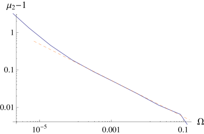
Figure 3: Scale-dependent variance of the projected stellar mass, with a power-law fit giving $\gamma=1.97$.

In Fig. 3 is the log-log plot of $\mu_{2}(\Omega)-1$ ($\Omega$ is normalized to the total solid angle from now onwards, unless the unit “steradian” appears explicitly). The exponent of the power-law fit of $\mu_{2}(\Omega)-1$ in $\Omega\in[8\cdot 10^{-5},8\cdot 10^{-2}]$ turns out to be somewhat large in absolute value, namely, $(\gamma-1)/2=0.486\pm 0.008$, giving $\gamma=1.97\pm 0.02$. In the fitted range, $\mu_{2}-1\ll 1$, while $\mu_{2}$ grows for small $\Omega$ and $\gamma$ tends to three, due to the effect of discreteness.

Therefore, in the range of $\Omega$ where the projected stellar mass distribution can be considered as a continuous mass distribution, it is quite uniform, with small fluctuations that are power-law correlated. The mass fluctuations are reduced by the projection, as explained in Sect. 5.1. Presumably, we can have a better representation of the correlation function for small $\Omega$ by suppressing the shot noise.

6.1 Shot noise suppression

The Poissonian fluctuations of an uncorrelated distribution of points in some volume are characterized by a number density variance equal to $1/N$, where $N$ is the mean number of points. This term is also present when the points are correlated. In the case of a distribution of particles with different masses, such as galaxies, and assuming that masses are statistically independent of positions, the shot noise term becomes

$$\frac{\langle m^{2}\rangle}{\langle m\rangle^{2}N}$$

(Peebles, 1993, pg. 509–510).

In the coarse multifractal analysis of a sample of $N$ particles, when the cell size is so small that no cell contains more than one particle and therefore the sums over cells and over particles coincide, the calculation of the moment ${\cal M}_{2}$ by Eq. (8) obtains the shot noise term

$$\frac{\sum m_{i}^{2}}{\left(\sum m_{i}\right)^{2}}=\frac{\langle m^{2}\rangle}{\langle m\rangle^{2}N}\,,$$ (20)

where the index $i$ of the sums runs over the set of particles. If we start with a cell size such that no cell contains more than one particle and let the size grow, then, at some point, some cells contain more than one particle and ${\cal M}_{2}$ grows, because the restricted sum over these cells is larger than the sum over the particles in the cells [for a cell with two particles, $(m_{1}+m_{2})^{2}>m_{1}^{2}+m_{2}^{2}$]. Therefore, the term (20) is the minimum value of ${\cal M}_{2}$, and while ${\cal M}_{2}$ stays constant, $D_{2}=0$, according to Eqs. (9) and (10). At some larger scale, ${\cal M}_{2}$ is definitely growing and there is a crossover to a scaling with $D_{2}>0$.

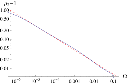
Figure 4: Values of $\mu_{2}(\Omega)-1$ after shot noise suppression, for the distributions of stellar mass, with linear fit (dashed line). It gives $\gamma=1.83$.

Peebles (1993) says about the shot noise term that “in most applications to be discussed here, this shot noise term is subdominant and will be dropped” and advises that, where the shot noise term is appreciable, it is to be subtracted. We subtract the shot noise term (20) from ${\cal M}_{2}(\Omega)$ and see the effect in Fig. 4, to be compared with Fig. 3. It is now possible to extend the power-law range to $\Omega\in[1.3\cdot 10^{-6},8\cdot 10^{-2}]$, with exponent $(\gamma-1)/2=0.415\pm 0.007$ (a long scaling range and a small error). This exponent gives $\gamma=1.83$, which agrees with the values found in Sect. 3. It also agrees with the results of Li and White (2009) and of Wang, Brunner and Dolence (2013) (the latter for galaxy positions). Their procedure for calculating the correlation function automatically suppresses the shot noise.

6.2 Finding the scale $r_{0}$

The scale $r_{0}$ can be found from the projected distribution by first finding the angular scale of homogeneity $\Omega_{0}$ in Eq. (19). According to Eq. (19), $\Omega_{0}$ is the solution of the equation $\mu_{2}(\Omega_{0})-1=1$. The scale of homogeneity of the three-dimensional distribution is found by expressing the mass variance $\mu_{2}(\Omega)-1$ as the average of $w(\theta)$, which is in turn given by Eq. (18). The equation that relates $\Omega_{0}$, $r_{0}/d_{*}$, $K$ and $\gamma$ follows from Eqs. (18) and (19) and writes

$${\Omega_{0}}^{(\gamma-1)/2}={\Omega}^{(\gamma-1)/2}\int\frac{d\Omega_{1}d\Omega_{2}}{\Omega^{2}}\,w(\theta_{12})$$

$$=K\left(\frac{r_{0}}{d_{*}}\right)^{\gamma}k_{\gamma}\int\frac{d\Omega_{1}d\Omega_{2}}{\Omega^{2}}\left(\frac{\theta_{12}}{\Omega^{1/2}}\right)^{1-\gamma}\,,$$ (21)

where $k_{\gamma}$ is the integral in Eq. (18), and the integral over $\Omega_{1}$ and $\Omega_{2}$ extends over a cell.

Given $\gamma$, the evaluation of $k_{\gamma}$ and the integral over $\Omega_{1}$ and $\Omega_{2}$ are straightforward numerical computations (for this integral, we take into account the small size of the relevant cells to ignore the spherical geometry and carry out the computation in the plane). To calculate the constant $K$, which is an integral that contains the luminosity function, we can use the Schechter model (Peebles, 1993). This model has two parameters, namely, the characteristic galaxy luminosity $L_{*}$ and the slope $\alpha$, but $K$ only depends on the latter. We take $\alpha\in(-1.2,-0.8)$, according to Zandivarez and Martínez (2011) and references therein.

To solve for $r_{0}/d_{*}$ we have to fix $\gamma$ and $\Omega_{0}$. Taking the value of $\gamma$ found in Sect. 6.1, we obtain that $\Omega_{0}=9.53\cdot 10^{-7}$ steradians. With $\gamma=1.83$, we compute that $k_{\gamma}=3.58$ and that the integral over $\Omega_{1}$ and $\Omega_{2}$ is $2.33$, while $K\in(0.89,1.17)$ (the uncertainties in $k_{\gamma}$ and the integral are negligible, in comparison). Employing Eq. (21) (and neglecting the uncertainty in $\Omega_{0}$), we obtain

$$r_{0}/d_{*}=0.0134\pm 0.0010$$

(where the uncertainty is small enough to assume that it is normally distributed).

To estimate the characteristic sample depth $d_{*}$, which is proportional to the square root of $L_{*}$, we take $M_{*}$, the absolute magnitude corresponding to $L_{*}$, to be

$$M_{*}-5\log_{10}\!h=-20.6\pm 0.2.$$

This value is based on the analysis of Zandivarez and Martínez (2011) and is in the interval of magnitudes of the most representative galaxies by mass density (Table 1). We obtain

$$d_{*} = 10\,\mathrm{pc}\times 10^{0.2(17.77+20.6\pm 0.2-5\log_{10}\!h)}$$

$$= (470\pm 40)\,\mathrm{Mpc}/h.$$

(the uncertainty is again small enough to assume that it is normally distributed). Hence,

$$r_{0}=(6.3\pm 0.7)\,\mathrm{Mpc}/h.$$

This is the clustering length of Eq. (1), in contrast with the (luminosity-dependent) homogeneity scale $v_{0}^{1/3}$ of Sect. 3, which is tailored to the sample geometry and coarse-graining method. The value of $r_{0}$ agrees with the value of Li and White (2009).

7 Summary and discussion

The standard scaling law of galaxy clustering is the power-law correlation function of galaxy positions, with canonical exponent $\gamma=1.8$ and clustering length $r_{0}\simeq 5\,h^{-1}$Mpc, which dates back over 50 years, since the early analyses of the galaxy-galaxy angular correlation function $w(\theta)$. We have shown that there are two important ingredients that are missing in most analyses of the galaxy distribution, namely, galaxy masses and relevant statistics other than the variance. Indeed, more important than the distribution of galaxy positions is the distribution of stellar mass, which is a proxy for the distribution of baryonic matter. Besides, statistics appropriate to describe strong galaxy clustering are the fractional moments, seldom employed. We have shown that a complete study of scaling laws of the distribution of stellar mass reveals novelties that are worth considering.

Our study is based on the theory of multifractal geometry. This theory assumes scaling laws for the growth of mass fluctuations on small scales, which define dimensions. The correlation dimension $D_{2}$, which is only one of many dimensions $D_{q}$, derives from the scaling the second-order statistical moment of the mass probability function. This moment also yields the scale of homogeneity. It is usually defined as the clustering length $r_{0}$, but a coarse-graining analysis obtains a volume $v_{0}$ (which depends somewhat on the method). In Sect. 2, we have seen that $v_{0}^{1/3}\simeq r_{0}$ but that the mass fluctuations at the scale $v_{0}$ are still considerable. A state of quasi-homogeneity is reached only for length scales that are almost an order of magnitude larger.

Conversely, the strong clustering regime, where fractal geometry applies, takes place for length scales that are almost an order of magnitude smaller, close to 1 Mpc. Unfortunately, there is not even one galaxy, on average, in a volume of such diameter; especially, if the volume is extracted from a volume-limited sample of galaxies. This leads to strong discreteness effects, which appear as errors in the calculation of $D_{2}$ and $v_{0}$. We have indeed shown that a strict definition of fractal scaling leads to considerable errors, namely, relative errors of 20% in $D_{2}$ and of 30% in $v_{0}^{1/3}$.

Nevertheless, a definition of scaling that encompasses the quasi-homogeneous regime leads to more precise results. The cell mass variance decreases in this regime yet the scaling continues, allowing us to calculate a precise scaling exponent $\gamma$. Although $\gamma$ is somewhat dependent on the volume-limited sample that we consider, its growth with luminosity is expected in a multifractal stellar mass distribution. Indeed, galaxy luminosity and stellar mass are strongly correlated and the stellar mass of a galaxy is correlated with the local dimension of the stellar mass distribution at its position. However, most stellar mass is concentrated in a restricted range of dimensions, namely, $D_{2}=1.2$–1.3 ($\gamma=1.7$–1.8), which is representative of the full stellar mass distribution. The homogeneity scale $v_{0}^{1/3}$ also grows with luminosity, being about $15\,h^{-1}$ Mpc for the set of galaxies that concentrates most of the mass.

It is to be remarked that the concentration of stellar mass in a range of galaxy luminosities that contains a small fraction of the galaxy number density makes the analysis of the stellar mass distribution a subject in its own right, quite different from the usual analysis of the galaxy number distribution. Nevertheless, the values of $\gamma$ and $r_{0}$ from both analyses are compatible (we recall our calculation of $r_{0}$ below). In this regard, we agree with the results of Li and White (2009).

The mass variance is not a sufficient statistic in the fractal regime and must be complemented with fractional moments $\mu_{q}$, for $q\in\mathbb{R}$, especially, $q\gtrsim 1$. The study of fractional moments confirms the multifractal nature of the stellar mass distribution but shows no way to redefine $q$-moments (with $q\neq 2$) that extends the multifractal scaling to the quasi-homogeneous regime. In this regime, fractional moments simply adopt the values that correspond to a Gaussian distribution, as shown using the lognormal model, which interpolates between strong clustering and homogeneity. The long scaling range of the mass variance, which goes across the transition to homogeneity into the quasi-homogeneous regime, is surely a consequence of its origin in the linear evolution of Gaussian initial conditions.

Even the comparatively long scaling range of the mass variance is limited to less than two orders of magnitude in length ($v^{1/3}$), as obtained from our volume-limited samples. This limitation is due to discreteness errors. In an attempt to reduce the discreteness errors, we study the angular distribution of the full flux-limited sample, which avails the $529\hskip 1.0pt967$ galaxies in our angular rectangle. However, in the calculation of $\mu_{2}(\Omega)-1$, many pairs of galaxies in a given angular region correspond to galaxies at very large distances, which are uncorrelated. So to speak, we enhance both the signal and the noise. After suppressing the shot noise, the range of scaling of the angular stellar mass distribution grows to $\Omega\in[2.5\cdot 10^{-6},1.6\cdot 10^{-1}]$ sr, with exponent $\gamma=1.83$. This range of $\Omega$, almost five orders of magnitude, is equivalent to a linear range of half of that, namely, two and half orders of magnitude.

From the angular scale of transition to homogeneity $\Omega_{0}$, it is possible to calculate $r_{0}$ by expressing $\Omega_{0}$ in terms of $r_{0}$ and several calculable magnitudes. In particular, this calculation involves the characteristic parameters of the galaxy luminosity function, which are somewhat uncertain. We obtain a reasonable value of $r_{0}$, in the range 5.8–$7.0\,h^{-1}$ Mpc.

To recapitulate and conclude, we have carried out a multifractal analysis of the stellar mass distribution, combining a set of volume-limited samples with the angular distribution. The methods developed here constitute an appealing alternative to other methods, such as methods that only use the galaxy positions or the two-point correlation function. Given that the important cosmological parameter $\sigma_{8}$ is theoretically defined in terms of the fluctuations of the full mass distribution, our methods can be relevant in the calculation of precision values of $\sigma_{8}$.

References

- Abazajian et al. (2009) Abazajian K.N. et al, The Seventh Data Release of the Sloan Digital Sky Survey, ApJS 182 (2009) 543–558.
- Borgani (1995) Borgani S., Scaling in the Universe, Rev. Mod. Phys. 251 (1995) 1–152.
-
Blanton et al. (2005)
Blanton M.R. et al,
New York University Value-Added Galaxy Catalog: A Galaxy Catalog Based on New Public Surveys, AJ 129 (2005) 2562–2578.
http://sdss.physics.nyu.edu/vagc NYU Value-Added Galaxy Catalog web page. - Blanton and Roweis (2007) Blanton M.R. and S. Roweis. K-Corrections and Filter Transformations in the Ultraviolet, Optical, and Near-Infrared, AJ 133 (2007) 734–754.
- Chacón-Cardona et al. (2016) Chacón-Cardona C.A., R.A. Casas-Miranda, J.C. Muñoz-Cuartas, Multi-fractal analysis and lacunarity spectrum of the dark matter haloes in the SDSS-DR7, Chaos, Solitons and Fractals 82 (2016) 22–33.
- Coleman and Pietronero (1992) Coleman P.H. and L. Pietronero, The fractal structure of the Universe, Phys. Rep. 213 (1992) 311–389.
- Coles and Jones (1992) Coles P. and B.J.T. Jones, A lognormal model for the cosmological mass distribution, MNRAS 248 (1991) 1–13.
- Davis and Peebles (1983) Davis, M. and P.J.E. Peebles, A survey of galaxy redshifts. V - The two-point position and velocity correlations, Astrophys. J. 267 (1983) 465–482.
- DES Collaboration (2018) DES Collaboration: Abbott et al., Dark Energy Survey Year 1 Results: Cosmological Constraints from Galaxy Clustering and Weak Lensing, Phys. Rev. D 98 043526 (2018).
- Durrer et al. (1997) Durrer R., J.-P. Eckmann, F. Sylos Labini, M. Montuori and L. Pietronero, Angular Projections of Fractal Sets, Europhysics Letters 40 (1997) 491–496.
- Falconer (2003) Falconer K., Fractal Geometry (Second Edition), John Wiley and Sons, Chichester, UK, (2003).
- Falconer, Fraser and Jin (2015) Falconer K., J.M. Fraser and Xiong Jin, Sixty years of fractal projections, in Fractal Geometry and Stochastics V, Progress in Probability 70, Birkhauser (2015), pg. 3–25 [arXiv:1411.3156].
- Gaite (2007) Gaite J., Halos and voids in a multifractal model of cosmic structure, Astrophys. J. 658 (2007) 11–24.
- Gaite (2018) Gaite J., Fractal analysis of the large-scale stellar mass distribution in the Sloan Digital Sky Survey, JCAP 2018, 07, 010.
- Gaite (2019) Gaite J., The Fractal Geometry of the Cosmic Web and Its Formation, Advances in Astronomy 2019, Article ID 6587138, 25 pages. https://doi.org/10.1155/2019/6587138.
- Gaite, Domínguez and Pérez-Mercader (1999) Gaite J., A. Domínguez and J. Pérez-Mercader, The fractal distribution of galaxies and the transition to homogeneity, Astrophys. J. 522 (1999) L5–L8.
- Geller and Huchra (1989) Geller M.J. and J.P. Huchra, Mapping the Universe, Science 246 (1989) 897–903.
- Groth and Peebles (1977) Groth E.J. and P.J.E. Peebles, Statistical analysis of catalogs of extragalactic objects. VII - Two- and three-point correlation functions for the high-resolution Shane-Wirtanen catalog of galaxies, Astrophys. J. 217 (1977) 385–405.
- Harte (2001) Harte D., Multifractals. Theory and applications, Chapman & Hall/CRC, Boca Raton, Fda. (2001).
- Hunt and Kaloshin (1997) Hunt B.R. and V.Y. Kaloshin, How projections affect the dimension spectrum of fractal measures, Nonlinearity 10 (1997) 1031–1046.
- Jones (2017) Jones B.J.T., Precision Cosmology: The First Half Million Years, Cambridge University Press (2017).
- Jones et al. (1988) Jones B.J.T., V. Martínez, E. Saar and J. Einasto, Multifractal description of the large-scale structure of the universe, Astrophys. J. 332 (1988) L1.
- Jones, Coles and Martínez (1992) Jones B.J.T., P. Coles and V. Martínez, Heterotopic clustering, MNRAS 259 (1992) 146–154.
- Jones et al. (2004) Jones B.J.T., V. Martínez, E. Saar and V. Trimble, Scaling laws in the distribution of galaxies, Rev. Mod. Phys. 76 (2004) 1211–1266.
- Kauffmann et al. (2003) Kauffmann G. et al, Stellar Masses and Star Formation Histories for Galaxies from the Sloan Digital Sky Survey, MNRAS 341 (2003) 33–53.
- Kofman et al. (1992) Kofman L., D. Pogosyan, S.F. Shandarin and A.L. Melott, Coherent structures in the universe and the adhesion model, The Astrophysical Journal 393 (1992) 437–449.
- Lahav and Liddle (2017) Lahav O. and A.R. Liddle, The Cosmological Parameters, in C. Patrignani et al. (Particle Data Group), Chin. Phys. C 40 (2016) [2017 update] 100001.
- Li and White (2009) Li Ch. and S.D.M. White, The distribution of stellar mass in the low-redshift Universe, MNRAS 398 (2009) 2177–2187.
- Mandelbrot (1983) Mandelbrot B.B., The fractal geometry of nature (rev. ed. of: Fractals, 1977), W.H. Freeman and Company (1983).
- Mitrinovic et al. (1993) Mitrinovic D.S., J.E. Pecaric and A.M. Fink, Classical and new inequalities in analysis, Kluwer, The Netherlands (1993).
- Peebles (1993) Peebles P.J.E., Principles of Physical Cosmology, Princeton University Press (1993).
- Pietronero (1987) Pietronero L., The fractal structure of the universe: Correlations of galaxies and clusters and the average mass density, Physica A 144 (1987) 257–284.
- Sarkar et al. (2009) Sarkar P., J. Yadav, B Pandey and S. Bharadwaj, The scale of homogeneity of the galaxy distribution in SDSS DR6, MNRAS 399 (2009) L128–31.
- Shao and Nikias (1993) Shao M. and C.-L. Nikias, Signal processing with fractional lower order moments, Proc. of the IEEE 81 (1993) 986–1010.
- Sylos Labini, Montuori and Pietronero (1998) Sylos Labini F., M. Montuori and L. Pietronero, Scale invariance of galaxy clustering, Phys. Rep. 293 (1998) 61–226.
- Sylos Labini, Vasilyev and Baryshev (2007) Sylos Labini F., NL Vasilyev and YV Baryshev, Power law correlations in galaxy distribution and finite volume effects from the Sloan Digital Sky Survey Data Release Four, Astron. Astrophys. 465 (2007) 23–33.
- Totsuji and Kihara (1969) Totsuji H. and T. Kihara, The Correlation Function for the Distribution of Galaxies, Publ. Astron. Soc. Japan 21 (1969) 221.
- Verevkin, Bukhmastova and Baryshev (2011) Verevkin A.O., Y.L. Bukhmastova and Y.V. Baryshev, The non-uniform distribution of galaxies from data of the SDSS DR7 survey, Astron Rep 55 (2011) 324–40.
- Wang, Brunner and Dolence (2013) Wang Y., R.J. Brunner and J.C. Dolence, The SDSS galaxy angular two-point correlation function, MNRAS 432 (2013) 1961–1979.
- Zandivarez and Martínez (2011) Zandivarez A. and H.J. Martínez, Luminosity function of galaxies in groups in the Sloan Digital Sky Survey Data Release 7: the dependence on mass, environment and galaxy type, MNRAS 415 (2011) 2553–2565.
- Zehavi et al. (2011) Zehavi I. et al, The luminosity and color dependence of the galaxy correlation function, The Astrophysical Journal 630 (2005) 1–27.