Excited-state quantum phase transition and the quantum speed limit time

Abstract

We investigate the influence of an excited-state quantum phase transition on the quantum speed limit time of an open quantum system. The system consists of a central qubit coupled to a spin environment modeled by a Lipkin-Meshkov-Glick Hamiltonian. We show that when the coupling between qubit and environment is such that the latter is located at the critical energy of the excited-state quantum phase transition, the qubit evolution shows a remarkable slowdown, marked by an abrupt peak in the quantum speed limit time. Interestingly, this slowdown at the excited-state quantum phase transition critical point is induced by the singular behavior of the qubit decoherence rate, being independent of the Markovian nature of the environment.

I Introduction

Quantum phase transitions are zero-temperature phase transitions in which a system ground state undergoes a qualitative variation once a Hamiltonian control parameter (such as an internal coupling constant or an external field strength) reaches a critical value. Quantum phase transitions are non-thermal and driven by quantum fluctuations in a many-body quantum system Carr (2010); Sachdev (2011); Dutta et al. (2015). They are the best-known example of criticality in quantum mechanics and, in the past decades, theoretical Emary and Brandes (2003); Zurek et al. (2005); Quan et al. (2006); Silva (2008); Dziarmaga (2010); Polkovnikov et al. (2011) and experimental Greiner et al. (2002); Bloch et al. (2008); Baumann et al. (2010) groups have paid much attention to this subject. Nowadays, quantum phase transitions are considered a keynote topic in many fields of quantum physics. In particular, ground state quantum phase transitions between different geometrical limits of algebraic models applied to nuclear and molecular structure have been extensively studied Gilmore (1979); Feng et al. (1981); Iachello and Zamfir (2004); Cejnar and Iachello (2007); Cejnar et al. (2010).

More recently, it has been found that the quantum phase transition concept, originally defined considering the system ground state, can be generalized and extended to the realm of excited states Cejnar et al. (2006); Cejnar and Stránský (2008); Caprio et al. (2008). A characteristic feature of excited-state quantum phase transitions is a discontinuity in the density of excited states at a critical value of the energy of the system. Such discontinuity, occurring at values of the control parameter other than the critical one, is a continuation at higher energies of the level clustering near the ground state energy that characterizes the ground state quantum phase transition Caprio et al. (2008); Leyvraz and Heiss (2005); Pérez-Fernández et al. (2009); Stránský et al. (2014). Establishing a parallelism with the Ehrenfest classification for ground state quantum phase transitions, excited-state quantum phase transitions can also be characterized by the nonanalytic evolution of the energy of an individual excited state of the system when varying the control parameter Caprio et al. (2008); Relaño et al. (2008); Pérez-Bernal and Iachello (2008); Pérez-Fernández et al. (2011a).

During the last decade, excited-state quantum phase transitions have been theoretically analyzed in various quantum many-body systems: the Lipkin-Meshkov-Glick (LMG) model Cejnar and Iachello (2007); Pérez-Fernández et al. (2009), the vibron model Caprio et al. (2008); Pérez-Bernal and Iachello (2008), the interacting boson model Cejnar and Jolie (2009), the kicked-top model Bastidas et al. (2014), and the Dicke model Pérez-Fernández et al. (2011a, b); Brandes (2013); Kloc et al. (2017) among others. Furthermore, the existence of a relation between excited-state quantum phase transitions and the onset of chaos has been explored in Ref. Pérez-Fernández et al. (2011b) and excited-state quantum phase transition signatures have been experimentally observed in superconducting microwave billiards Dietz et al. (2013), different molecular systems Larese and Iachello (2011); Larese et al. (2013), and spinor Bose-Einstein condensates Zhao et al. (2014). The excited-state quantum phase transition influence on the dynamics of quantum systems has recently attracted significant attention and several remarkable dynamical effects of excited-state quantum phase transitions have been revealed Relaño et al. (2008); Pérez-Fernández et al. (2009, 2011a); Santos and Pérez-Bernal (2015); Santos et al. (2016); Pérez-Bernal and Santos (2017); Wang and Quan (2017); Engelhardt et al. (2015); Puebla et al. (2013); Puebla and Relaño (2015); Kloc et al. (2018). In particular, the impact of excited-state quantum phase transitions on the adiabatic dynamics of a quantum system has been recently analyzed Kopylov et al. (2017), as well as the relationship between thermal phase transitions and excited-state quantum phase transitions Pérez-Fernández and Relaño (2017).

On the other hand, due to fast progresses in the fields of quantum computation and quantum information science, the achievement of fast and controlled evolution of quantum systems is a need of the hour. As a fundamental bound, imposed by quantum mechanics, on the evolution speed of a system, the quantum speed limit time is in the spotlight and its study has drawn considerable attention both in isolated and open quantum systems Deffner and Lutz (2013); Taddei et al. (2013); del Campo et al. (2013); Zhang et al. (2014); Sun et al. (2015); Liu et al. (2016); Marvian et al. (2016); Ektesabi et al. (2017); Cai and Zheng (2017) (many more references can be found in the recent reviews Frey (2016); Deffner and Campbell (2017)). The quantum speed limit time, whose origin can be traced back to the reinterpretation of the Heisenberg time-energy uncertainty relation by Mandelstam and Tamm Mandelstam and Tamm (1945), is defined as the minimum evolution time required by a quantum system to evolve between two distinct states Brody (2003); Deffner and Lutz (2013); Frey (2016). The quantum speed limit time sets a lower bound to the time needed to evolve between two distinguishable states of a given system, and thus provides qualitative information about the time evolution of a system without explicitly solving the system dynamics Pfeifer and Fröhlich (1995).

Nowadays, the quantum speed limit time is a quantity that has a growing importance in quantum physics. In fact, it has been used to set fundamental limits to the speed of computing devices Lloyd (2000), to the performance of quantum control Caneva et al. (2009), and to the entropy production rate in nonequilibrium quantum thermodynamics Deffner and Lutz (2010); to best parameter estimation in quantum metrology Giovannetti et al. (2011); Braun et al. (2018); and to analyze information scrambling del Campo et al. (2017). See Frey (2016); Deffner and Campbell (2017) and references therein for a more exhaustive list of applications of the quantum speed limit. Moreover, the quantum speed limit may help us figuring out how to control and manipulate quantum coherence Cai and Zheng (2017). For a given evolution time, the ratio between the quantum speed limit time and the driving time provides an estimation of the potential capacity for speeding up the quantum dynamic evolution. Namely, a ratio equals to $1$ indicates that there is no room for further acceleration, but if the ratio is less than $1$, the smaller the ratio, the larger the possible system evolution speed up Deffner and Campbell (2017); Liu et al. (2015). Interestingly, there is a common belief that the quantum speed limit is a strictly quantum phenomenon, without a classical counterpart. However, speed limit bounds in classical systems, in close connection with the quantum speed limit, have been recently reported Shanahan et al. (2018); Okuyama and Ohzeki (2018).

For open quantum systems, one can expect that decoherence effects that stem from the interaction between the system and the environment will strongly influence the quantum speed limit. It has already been shown that the system decoherence can be enhanced by the occurrence of quantum criticality in the environment Quan et al. (2006); Relaño et al. (2008). Hence, one would naturally expect an important variation in the quantum speed limit time whenever the environment undergoes a quantum phase transition. Indeed, recent results obtained for open systems consisting of a qubit coupled to a spin $\frac{1}{2}$ XY chain with nearest neighbors interaction Wei et al. (2016) or to a LMG bath Hou et al. (2016) clearly verify that the quantum speed limit time has a remarkable variation in the critical point of the environment ground state quantum phase transition. This happens to such an extent that the quantum speed limit time has been proposed as a possible probe to detect the occurrence of ground state quantum phase transitions Wei et al. (2016); Hou et al. (2016).

In this work, we extend the results obtained for ground state quantum phase transitions in Refs. Wei et al. (2016); Hou et al. (2016) to excited states and excited-state quantum phase transitions; to study the relationship between criticality in excited-state quantum phase transitions and the quantum speed limit. With this aim, we analyze the quantum speed limit time of an open system that consists of a central qubit coupled to a LMG environment Lipkin et al. (1965). The net effect of the coupling between the central spin and its environment is a change of the environment Hamiltonian control parameter Cucchietti et al. (2007); Relaño et al. (2008); Pérez-Fernández et al. (2009); Rossini et al. (2007). Therefore, the variation of the coupling strength can drive the environment through the critical point of an excited-state quantum phase transition. In this case we report the effects that the crossing has on the quantum speed limit time. Furthermore, since the Markovian nature of the environment has a strong influence on the properties of the quantum speed limit, we will also study how the excited-state quantum phase transition affects the environment’s Markovian nature, looking for a deeper understanding on the relationship between excited-state quantum phase transitions and the quantum speed limit time.

The rest of this article is organized as follows. In Sec. II, we introduce the quantum speed limit for open systems and shortly review some key concepts, due to the nontrivial way of addressing the concept of quantum speed limit for such systems. In Sec. III, we describe the model, consisting of a central qubit coupled to the LMG model, and analyze the phase transitions of the environment, especially those related to excited-state quantum phase transitions. In Sec. IV we define the qubit quantum speed limit time and investigate how the excited-state quantum phase transition affects this quantity. Sec. V is devoted to the search of a physical explanation for the singular behavior of the quantum speed limit time at the critical point of the excited-state quantum phase transition. We discuss in this section how the variation of the quantum speed limit time at the excited-state quantum phase transition critical point stems from the singular behavior of the qubit decoherence rate and not from the Markovian nature of the environment. Finally, we discuss and summarize our results in Sec. VI. We have included an Appendix where we prove several equations that are used in the main text.

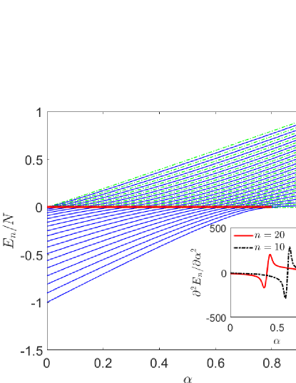
Figure 1: Energy levels of the environment Hamiltonian (9) as a function of the control parameter $\alpha$ with $N=40$. Odd (even) parity levels are depicted with blue solid (green dot-dashed) curves. The thick red line indicates the critical energy, $E_{c}=0$, of the excited-state quantum phase transition. Inset: The second derivative of the level energy with respect to the variable $\alpha$ for the $10$th and $20$th excited states, respectively.

II The quantum speed limit in open systems

In this section we briefly review the key concepts of the quantum speed limit in open systems and establish the notions and the notation that will be used in the rest of this article. We follow the approach presented in Refs. Deffner and Lutz (2013); Deffner and Campbell (2017), where the quantum speed limit for a driven open system is obtained using a geometric approach.

Consider a driven open quantum system with initial state $\rho_{0}$, its evolution is governed by the quantum master equation Deffner and Lutz (2013); Breuer and Petruccione (2007)

$$\dot{\rho}_{t}=L_{t}(\rho_{t}),$$ (1)

where $L_{t}$ is an arbitrary Liouvillian superoperator and the dot denotes the time derivative. The quantum speed limit time is derived as a lower bound to the evolution time between an initial state $\rho_{0}$ and a final state $\rho_{t}$, which can be obtained with Eq. (1). In the geometric approach the distance between two quantum states is measured by the Bures angle Deffner and Lutz (2013); Jozsa (1994)

$$\mathcal{L}(\rho_{0},\rho_{t})=\arccos\left(\sqrt{F(\rho_{0},\rho_{t})}\right),$$ (2)

where $F(\rho_{0},\rho_{t})=[\mathrm{tr}(\sqrt{\rho_{t}}\rho_{0}\sqrt{\rho_{t}})]^{2}$ is the quantum fidelity between $\rho_{0}$ and $\rho_{t}$. According to Eq. (2), the Bures angle is a measure of the distance between states and the quantum speed limit can be interpreted as the the maximum possible speed to sweep out the angle $\mathcal{L}(\rho_{0},\rho_{t})$ under the dynamics governed by Eq. (1) Shanahan et al. (2018). The expression of the quantum speed limit, $\nu$, can therefore be obtained by taking the time derivative of the Bures angle

$$\nu=\dot{\mathcal{L}}(\rho_{0},\rho_{t})\leq|\dot{\mathcal{L}}(\rho_{0},\rho_{t})|.$$ (3)

This is a cumbersome operation in the general case, as it involves square roots of operators, but using the definition (2) and after some algebra, the above inequality can be written as Deffner and Lutz (2013).

$$2\cos[\mathcal{L}(\rho_{0},\rho_{t})]\sin[\mathcal{L}(\rho_{0},\rho_{t})]\dot{\mathcal{L}}(\rho_{0},\rho_{t})\leq|\dot{F}(\rho_{0},\rho_{t})|.$$ (4)

For an initial state that is pure, $\rho_{0}=|\psi_{0}\rangle\langle\psi_{0}|$, and making use of the von Neumann and Cauchy-Schwarz inequalities, inequality (4) can be further simplified as Deffner and Lutz (2013)

$$2\cos[\mathcal{L}(\rho_{0},\rho_{t})]\sin[\mathcal{L}(\rho_{0},\rho_{t})]\dot{\mathcal{L}}(\rho_{0},\rho_{t})\leq|\langle\psi_{0}|\dot{\rho}_{t}|\psi_{0}\rangle|$$

$$\leq\mathrm{min}\{||L_{t}(\rho_{t})||_{1},||L_{t}(\rho_{t})||_{2},||L_{t}(\rho_{t})||_{\infty}\},$$ (5)

where Eq. (1) has been used to get the second inequality and $||\mathcal{B}||_{p}=\left(\sum_{k}b_{k}^{p}\right)^{1/p}$ with $b_{k}$ is the $k$th singular value of $\mathcal{B}$ denoting the Schatten $p$ norm of the operator $\mathcal{B}$. The cases $p=1,2,\infty$ correspond with the trace norm, the Hilbert-Schmidt norm, and the operator norm, respectively.

Integrating Eq. (II) over time from $t=0$ to $t=\tau_{e}$, we can obtain the quantum speed limit time $\tau_{e}\geq\mathrm{max}\{\tau_{1},\tau_{2},\tau_{\infty}\}$ where $\tau_{p}=\sin^{2}[\mathcal{L}(\rho_{0},\rho_{\tau_{e}})]/\Gamma_{\tau_{e}}^{p}$ with $\Gamma_{\tau_{e}}^{p}=(1/\tau_{e})\int_{0}^{\tau_{e}}dt||L_{t}(\rho_{t})||_{p}$ and $p=1,2,\infty$. Then, a unified expression of the quantum speed limit time for generic open system dynamics can be defined as

$$\tau_{\mathrm{QSL}}=\mathrm{max}\left\{\frac{1}{\Gamma_{\tau_{e}}^{1}},\frac{1}{\Gamma_{\tau_{e}}^{2}},\frac{1}{\Gamma_{\tau_{e}}^{\infty}}\right\}\sin^{2}\left[\mathcal{L}(\rho_{0},\rho_{\tau_{e}})\right].$$ (6)

Here, we stress that the derivation of Eq. (6) assumes a pure initial state and it cannot be applied to mixed initial states. Properly formulating the quantum speed limit time for mixed initial states is a delicate issue which is still under study Zhang et al. (2014); Sun et al. (2015); Pires et al. (2016); Ektesabi et al. (2017).

The quantum speed limit time was experimentally investigated in a cavity QED system via the second order intensity correlation function and observing the speed up of the system evolution under environment changes Cimmarusti et al. (2015). Nevertheless, a direct experimental estimation of the quantum speed limit time itself is still an open problem. It is noteworthy that a possible procedure to test the quantum speed limit time in quantum interferometry has been recently proposed Mondal and Pati (2016).

III Model

We consider a system composed by a qubit coupled to a spin environment. The Hamiltonian of the total system is Quan et al. (2006); Cucchietti et al. (2007); Pérez-Fernández et al. (2009)

$$\hat{H}=\hat{H}_{\mathcal{E}}+\hat{H}_{\mathcal{SE}},$$ (7)

where $\hat{H}_{\mathcal{E}}$ is the environment Hamiltonian and the interaction between qubit and environment is modeled by $\hat{H}_{\mathcal{SE}}$, which can be written as Relaño et al. (2008); Pérez-Fernández et al. (2009)

$$\hat{H}_{\mathcal{SE}}=|0\rangle\langle 0|\otimes\hat{H}_{0}+|1\rangle\langle 1|\otimes\hat{H}_{1},$$ (8)

where, $|0\rangle$ and $|1\rangle$ denote the two components of the qubit, while $\hat{H}_{0}$ and $\hat{H}_{1}$ are interaction Hamiltonians that act upon the environment Hilbert space. Therefore, depending on the particular qubit state, the environment evolution takes place under a different effective Hamiltonian $\hat{H}_{\mathcal{E}}^{l}=\hat{H}_{\mathcal{E}}+\hat{H}_{l}$ with $l=0,1$. As we will see below, the effect of $\hat{H}_{l}$ is to change the strength of the second term in the environment Hamiltonian (9). Therefore, varying the interaction Hamiltonian $\hat{H}_{l}$, one can drive the environment through its critical point Relaño et al. (2008); Pérez-Fernández et al. (2009).

Specifically, the environment in our study is given by the generalized LMG model. This model, originally introduced as a toy model in nuclear structure to test the validity of different approximations Lipkin et al. (1965), has been recently extensively used to study excited-state quantum phase transitions Relaño et al. (2008); Pérez-Fernández et al. (2009); Santos et al. (2016); Šindelka et al. (2017) and has been implemented in the laboratory making use of different platforms: trapped ions Monz et al. (2011); Lanyon et al. (2011), large-spin molecules Gatteschi and Sessoli (2003), Bose-Einstein condensates Albiez et al. (2005); Gross et al. (2010); Riedel et al. (2010), optical cavities Leroux et al. (2010), and cold atoms Makhalov et al. (2019). The LMG model Hamiltonian is

$$\hat{H}_{\mathcal{E}}=-\frac{4(1-\alpha)}{N}\hat{S}_{x}^{2}+\alpha\left(\hat{S}_{z}+\frac{N}{2}\right),$$ (9)

where $N$ is the size of the environment, the control parameter $0\leq\alpha\leq 1$ denotes the strength of the magnetic field along the $z$ direction, and $\hat{S}_{\gamma}=\sum_{j=1}^{N}\hat{\sigma}_{\gamma}^{j}$, the sum of Pauli spin matrices $\hat{\sigma}_{\gamma}$ for $\gamma=\{x,y,z\}$.

The total spin in the LMG model is a conserved quantity, i.e., $[\hat{H}_{\mathcal{E}},\hat{\mathbf{S}}^{2}]=0$ Dusuel and Vidal (2005). In our study, only the maximum spin sector $S=N/2$ will be considered. Therefore, the dimension of the Hamiltonian matrix is $\mathrm{Dim}[H]=N+1$. Moreover, as the Hamiltonian (9) conserves parity, the parity operator, $\Pi=(-1)^{S+m}$ with $m$ is the eigenvalue of $\hat{S}_{z}$, split the Hamiltonian matrix into even- and odd-parity blocks, with dimension $\mathrm{Dim}[H_{\mathcal{E}}]_{\mathrm{even}}=N/2+1$ and $\mathrm{Dim}[H_{\mathcal{E}}]_{\mathrm{odd}}=N/2$ Santos et al. (2016). In this work, we only consider even parity states, the subset that includes the ground state. We should point out that for simplicity, we consider $\hbar=1$ throughout this article and set the quantities in our study as unitless.

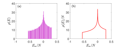
Figure 2: (a) Density of states of the environment Hamiltonian (9) for $N=2000$ with $\alpha=0.3$. (b) Normalized density of states of $\hat{H}_{\mathcal{E}}$, calculated by means of Eq. (10), with $N=2000$ and $\alpha=0.3$.

III.1 Phase transitions in the environment

It is well known that the LMG model Hamiltonian in Eq. (9) exhibits a second-order ground state quantum phase transition at a critical value of the control parameter $\alpha_{c}=0.8$ Relaño et al. (2008); Pérez-Fernández et al. (2009); Romera et al. (2014); Šindelka et al. (2017). The phase with $\alpha>\alpha_{c}$ is the symmetric phase, while the broken-symmetry phase corresponds to control parameter values $\alpha<\alpha_{c}$ Pérez-Fernández et al. (2009). However, besides the ground state quantum phase transition, the Hamiltonian (9) also displays an excited-state quantum phase transition and the signatures of the ground state quantum phase transition, e.g., the nonanalytical evolution of the ground state as the control parameter of the system is varied, propagates to excited states for a control parameter value $\alpha<\alpha_{c}$, i.e., in the broken-symmetry phase.

The LMG model correlation energy diagram is shown in Fig. 1, depicting energy levels as a function of the control parameter $\alpha$ for $\hat{H}_{\mathcal{E}}$ with $N=40$. In this figure it can be easily noticed how pairs of eigenstates with different parity are degenerate for $E<0$, and nondegenerate when $E>0$. Moreover, the energy gap between adjacent energy levels approaches zero around $E\approx 0$ in the broken-symmetry phase, where energy levels concentrate around $E=0$, marking the high local energy level density that characterizes excited-state quantum phase transitions. Each excited energy level has an inflection point at $E\approx 0$ Caprio et al. (2008) that induces a singular behavior in the second derivative of every individual excited state energy with respect to the control parameter $\alpha$ (see the inset of Fig. 1) Pérez-Bernal and Iachello (2008). A true nonanalytic behavior only happens in the large $N$ limit, also called thermodynamic or mean field limit, but even for systems of finite size ($N=40$, as in Fig. 1), there are clear precursors of the excited-state quantum phase transition effects, like the behavior of $\partial^{2}E_{n}/\partial\alpha^{2}$ for $n>0$ Pérez-Bernal and Iachello (2008). Something similar happens for the ground state energy, the $n=0$ case, that shows a discontinuity at the critical value of the control parameter, $\alpha_{c}$, associated with the ground state quantum phase transition. The excited-state quantum phase transition can be crossed in two ways: varying the energy for a fixed parameter value $\alpha<\alpha_{c}$ or choosing an excited state and varying the control parameter. It is important to understand that different excited states cross the excited-state quantum phase transition at different values of the control parameter $\alpha$, as shown in the inset of Fig. 1.

For a given control parameter value $\alpha<\alpha_{c}$, the piling of energy levels at $E\approx 0$ that marks the excited-state quantum phase transition will lead, in the large $N$ limit, to a discontinuity in the density of states. Indeed, as shown in Fig. 2(a), around $E=0$ the density of states $\rho(E)$ of $\hat{H}_{\mathcal{E}}$ has a peak for finite $N$, which will transform to a logarithmic divergence as $N\to\infty$ Caprio et al. (2008); Ribeiro et al. (2008). Therefore, the critical energy of the environment (9) is $E_{c}=0$ and, in fact, excited-state quantum phase transitions are often characterized by the singular behavior of the density of states occuring at the critical energy $E_{c}$, for fixed values of the control parameter Caprio et al. (2008); Pérez-Fernández et al. (2009); Santos et al. (2016); Leyvraz and Heiss (2005); Stránský et al. (2014). The divergence of the density of states at $E_{c}=0$ can be understood using a semiclassical approach or the coherent state approach Caprio et al. (2008).

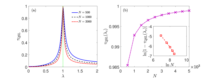
Figure 3: (a) The quantum speed limit time of the qubit as a function of the coupling strength $\lambda$ for different environment sizes ($N$ values) for a system with a control parameter $\alpha=0.4$. The actual evolution time is set to unity, $\tau_{e}=1$. The vertical green dotted line indicates the critical value of the Hamiltonian parameter $\lambda_{c}$ obtained from Eq. (14). (b) The critical quantum speed limit time $\tau_{\mathrm{QSL}}(\lambda_{c})$ as a function of the environment size, $N$, with $\alpha=0.4$ and $\tau_{e}=1$. Inset: $1-\tau_{\mathrm{QSL}}(\lambda_{c})$ as a function of $N$, in a double logarithmic scale.

In the semiclassical limit, the quantum expression for the density of states $\rho(E)=\sum_{j}(E-E_{j})$ can be decomposed into a smooth and an oscillatory component Gutzwiller (1990), $\rho(E)=\bar{\rho}(E)+\tilde{\rho}(E)$. The smooth part, $\bar{\rho}(E)$, is given by the classical phase space integral, while the oscillatory term, $\tilde{\rho}(E)$, can be expressed as a sum over classical periodic orbits Gutzwiller (1990). In the classical limit, the oscillatory part can be omitted Pérez-Fernández et al. (2011a). Then the density of states of the environment (9) has the following form

$$\rho(E)=\bar{\rho}(E)=\left(\frac{N}{2\pi}\right)\int\delta[E-\mathcal{H}(x,p)]dxdp,$$ (10)

where the environment’s classical counterpart Hamiltonian $\mathcal{H}(x,p)$ can be obtained via the coherent or intrinsic state approach Pérez-Fernández et al. (2009, 2011a). Equation (10) shows that the divergence in the density of states stems from the nonanalytical dependence of the classical phase space volume on the energy. In addition, such nonanalyticity is usually associated with stationary points of the classical Hamiltonian Pérez-Fernández et al. (2011a); Stránský et al. (2014); Heiss and Müller (2002).

In Fig. 2(b), we plot the smooth part of the environment density of states for Hamiltonian (9) as a function of the eigenenergies. Note that the density of states has been normalized by the size of the environment. Obviously, the density of states exhibits a cusp singularity (i.e., an infinite peak) at $E_{c}=0$. Therefore, we confirm that the critical energy of excited-state quantum phase transition is located at $E_{c}=0$. Moreover, a very good agreement between Figs. 2(a) and 2(b) can be clearly appreciated.

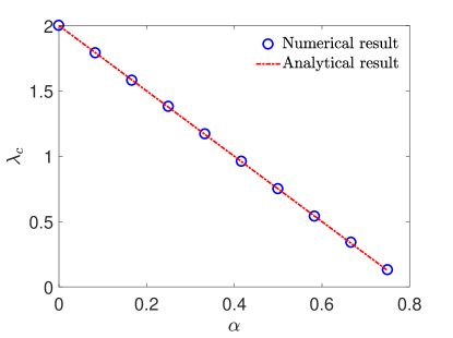
Figure 4: Critical coupling strength, $\lambda_{c}$, as a function of $\alpha$ with $\tau_{e}=1$ and an environment size $N=1000$. The numerical result is obtained by identifying the location of the maximum point in $\tau_{\mathrm{QSL}}$, while the analytical result is provided by Eq. (14).

III.2 The critical coupling

In our study, the qubit is coupled to the environment (9) with an interaction term

$$\hat{H}_{\mathcal{SE}}=\lambda\sigma_{\mathcal{S}}^{z}\hat{S}_{z},$$ (11)

where $\lambda$ is the coupling strength and $\sigma_{\mathcal{S}}^{z}$ is the qubit Pauli matrix. Following Refs. Quan et al. (2006); Pérez-Fernández et al. (2009), we assume that the qubit is coupled with the environment only in the $|1\rangle$ state. Then, according to Eq. (8), the effective Hamiltonian of the environment has the following expressions Pérez-Fernández et al. (2009)

$$\hat{H}_{\mathcal{E}}^{0} = -\frac{4(1-\alpha)}{N}\hat{S}_{x}^{2}+\alpha\hat{S}_{z},$$ (12)

$$\hat{H}_{\mathcal{E}}^{1} = -\frac{4(1-\alpha)}{N}\hat{S}_{x}^{2}+(\alpha+\lambda)\hat{S}_{z},$$ (13)

when the qubit is in state $|0\rangle$ and $|1\rangle$, and where irrelevant constant terms have been ommited. It can be seen that the qubit coupling to the environment is such that the two states of the qubit induce two different strengths in the second term of the environment Hamiltonian.

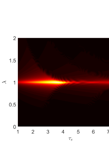
Figure 5: The quantum speed limit time, $\tau_{\mathrm{QSL}}$, as a function of the evolution time, $\tau_{e}$, and the coupling strength, $\lambda$, with a control parameter $\alpha=0.4$ and an environment size $N=1000$.

The variation of the coupling strength $\lambda$ can drive the environment through the critical point of the ground state quantum phase transition. The interplay between the quantum criticality of the environment and the quantum speed limit time of the qubit has been analyzed in this case Wei et al. (2016); Hou et al. (2016) and it has been found that the ground state quantum phase transition of the environment substantially diminishes the speed of evolution of the qubit. Our aim in the present work is, however, to assess the effect of the environment excited-state quantum phase transition on the quantum speed limit time of the qubit. To this end, we need to know, for a control parameter $\alpha$ and critical energy $E_{c}$, the critical value of the coupling parameter –denoted as $\lambda_{c}$– that will make the environment reach the critical energy $E_{c}$ of the excited-state quantum phase transition.

In general, the critical energy of an excited-state quantum phase transition is a function of the control parameter and the value of the critical coupling has to be obtained numerically for any initial state Pérez-Fernández et al. (2009, 2011a). However, for the LMG bath (9), the critical energy is independent of the control parameter $\alpha$ as can be seen in Fig. 1. When the initial state of environment is the ground state, the critical value of the coupling $\lambda_{c}$ can be derived using the intrinsic state formalism Relaño et al. (2008)

$$\lambda_{c}=2-\frac{5}{2}\alpha.$$ (14)

We would like to emphasize that the critical coupling $\lambda_{c}$, which induces the excited-state quantum phase transition in the environment Hamiltonian (9), differs from $\lambda_{c0}$, the critical coupling for the ground state quantum phase transition Pérez-Fernández et al. (2009, 2011a).

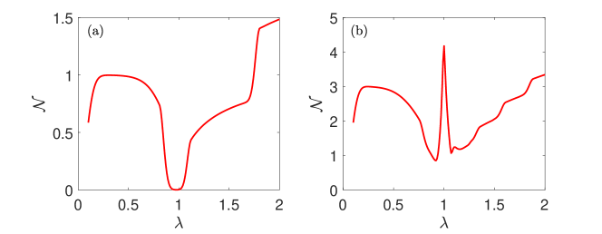
Figure 6: The non-Markovianity $\mathcal{N}$ as a function of coupling strength $\lambda$ for $\alpha=0.4$ and environment size $N=1000$, with evolution time values $\tau_{e}=3.5$ (a) and $\tau_{e}=8$ (b).

IV Quantum speed limit time of the qubit

To understand the effects of the excited-state quantum phase transition on the quantum speed limit, we study the quantum speed limit time of the qubit after a quench with a coupling strength value such that it drives the environment through the critical energy of the excited-state quantum phase transition. The initial state of the qubit is defined as $|\psi_{0}\rangle=\cos(\theta/2)|0\rangle+e^{-i\phi}\sin(\theta/2)|1\rangle$, while the environment is assumed to be initially in the ground state of $\hat{H}_{\mathcal{E}}^{0}$: $|\Psi^{0}_{\mathcal{E},G}\rangle$. Therefore, the wave function of the total system at $t=0$ is $|\Phi(0)\rangle=[\cos(\theta/2)|0\rangle+e^{-i\phi}\sin(\theta/2)|1\rangle]\otimes|\Psi^{0}_{\mathcal{E},G}\rangle$. The total system wave function evolves in time according to the Schrödinger equation and the state of the total system at time $t$ is

$$|\Phi(t)\rangle=\cos(\theta/2)|0\rangle\otimes|\Psi^{0}_{\mathcal{E}}(t)\rangle+e^{-i\phi}\sin(\theta/2)|1\rangle\otimes|\Psi^{1}_{\mathcal{E}}(t)\rangle,$$ (15)

where the evolution of the environmental states $|\Psi^{0}_{\mathcal{E}}(t)\rangle$ and $|\Psi^{1}_{\mathcal{E}}(t)\rangle$ satisfies the Schrödinger equation $i\partial_{t}|\Psi^{l}_{\mathcal{E}}(t)\rangle=\hat{H}_{\mathcal{E}}^{l}|\Psi_{\mathcal{E}}^{l}(t)\rangle$, with $\hat{H}_{\mathcal{E}}^{l}$ for $l=0,1$ is given by Eqs. (12) and (13), respectively. The evolution of the qubit, therefore, depends on the dynamics of the two environment branches evolving with effective Hamiltonians $\hat{H}_{\mathcal{E}}^{0}$ and $\hat{H}_{\mathcal{E}}^{1}$.

From Eq. (15), the reduced density matrix of the qubit in the $\{|0\rangle,|1\rangle\}$ basis at time $t$ is

$$\rho_{S}(t) =\mathrm{Tr}_{\mathcal{E}}|\Phi(t)\rangle\langle\Phi(t)|$$

$$=\begin{bmatrix}\cos^{2}(\theta/2)&\frac{1}{2}e^{i\phi}\sin(\theta)\mathcal{M}^{\ast}(t)\\ \frac{1}{2}e^{-i\phi}\sin(\theta)\mathcal{M}(t)&\sin^{2}(\theta/2)\end{bmatrix},$$ (16)

where $\mathcal{M}(t)=\langle\Psi^{0}_{\mathcal{E},G}|e^{i\hat{H}_{\mathcal{E}}^{0}t}e^{-i\hat{H}_{\mathcal{E}}^{1}t}|\Psi^{0}_{\mathcal{E},G}\rangle$ is the decoherence factor. The modulus square of $\mathcal{M}(t)$ is known as the Loschmidt echo (LE), which has been widely studied in many fields (see, e.g., Ref. Gorin et al. (2006) and references therein). In the present work, we set the energy of the initial state $|\Psi^{0}_{\mathcal{E},G}\rangle$ to zero and the decoherence factor $\mathcal{M}(t)$ in Eq. (16) is reduced to

$$\mathcal{M}(t)=\langle\Psi_{\mathcal{E},G}^{0}|e^{-i\hat{H}_{\mathcal{E}}^{1}t}|\Psi_{\mathcal{E},G}^{0}\rangle,$$ (17)

that can be identified with the survival probability of the initial quantum state $|\Psi_{\mathcal{E},G}^{0}\rangle$ evolving under the quenched Hamiltonian $\hat{H}_{\mathcal{E}}^{1}$.

In the rest of this section we investigate what happens to the quantum speed limit time of the qubit when the environment undergoes an excited-state quantum phase transition. We show how signatures of the excited-state quantum phase transition manifest themselves in the quantum speed limit time of the qubit after quenching the coupling strength between qubit and environment in such a way that the environment passes through the critical point of the excited-state quantum phase transition.

From Eq. (16), the quantum speed limit time (6) for the qubit evolution from $t=0$ to $t=\tau_{e}$ can be expressed as (see the appendix for the details)

$$\tau_{\mathrm{QSL}}=\frac{\sin(\theta)\{1-\mathfrak{R}[\mathcal{M}(\tau_{e})]\}}{(1/\tau_{e})\int_{0}^{\tau_{e}}dt|\partial_{t}\mathcal{M}(t)|},$$ (18)

where $\mathfrak{R}[\mathcal{M}(\tau_{e})]$ denotes the real part of $\mathcal{M}(t)$ at $t=\tau_{e}$. In the following, without loss of generality, we set $\theta=\pi/2$.

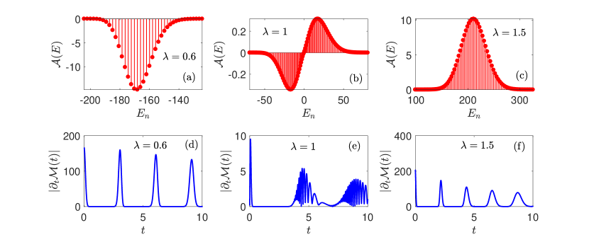
Figure 7: $\mathcal{A}(E)$ and $|\partial_{t}\mathcal{M}(t)|$ for different coupling strengths for an environment with control parameter $\alpha=0.4$ and size $N=1000$. (a)-(c): $\mathcal{A}(E)$ as a function of $E_{n}$ [see Eq. (22)] with $\lambda$ below (a), at (b), and above (c) the critical coupling strength, respectively. Panels (d)-(f) represent the evolution of $|\partial_{t}\mathcal{M}(t)|$ calculated from Eq. (21) for the same coupling parameter values.

We depict in Fig. 3(a) the quantum speed limit time of the qubit as a function of the coupling strength $\lambda$. For the sake of simplicity, we set the evolution time $\tau_{e}=1$. This figure has several remarkable features. On the one hand, when the value of the coupling strength is far away from the critical value $\lambda_{c}$, the quantum speed limit time is small. Moreover, increasing the environment size $N$, the evolution of the qubit can be accelerated. On the other hand, it can be clearly noticed in the figure how the quantum speed limit time displays a sharp peak at the critical coupling value $\lambda_{c}$, which implies that driving the environment through the excite-state quantum phase transition results in a slowdown of the quantum evolution of the qubit. The cusplike shape of the quantum speed limit time in the vicinity of the critical coupling becomes sharper as the environment size $N$ increases. Finally, the value of the quantum speed limit time at $\lambda_{c}$, i.e., the critical quantum speed limit time $\tau_{\mathrm{QSL}}(\lambda_{c})$, is very close to the actual evolution time and is independent of the size of environment $N$.

In Fig. 3(b) we show how the critical quantum speed limit time $\tau_{\mathrm{QSL}}(\lambda_{c})$ changes with the environment size $N$, again for $\alpha=0.4$ and $\tau_{e}=1$. It is obvious that $\tau_{\mathrm{QSL}}(\lambda_{c})$ increases and tends to the actual evolution time for increasing $N$. By using the least square method, we find that the relation between $\tau_{\mathrm{QSL}}(\lambda_{c})$ and $N$ is approximately $1-\tau_{\mathrm{QSL}}(\lambda_{c})=N^{-\mu}$ [cf. the inset of Fig. 3(b)] with $\mu\approx 1$. Therefore, $\tau_{\mathrm{QSL}}(\lambda_{c})\to\tau_{e}$ in the thermodynamic limit $N\to\infty$.

The features observed in the two panels of Fig. 3 indicate that the quantum speed limit time can be used as a proxy for excited-state quantum phase transitions in the environment. To further verify this statement, we compare the numerically estimated critical coupling strength, obtained as the location of the maximum in $\tau_{\mathrm{QSL}}$, with the exact value of $\lambda_{c}$ in Eq. (14). The results are displayed in Fig. 4, with a very good agreement between numerical and analytical results, evidencing that the qubit quantum speed limit time may be considered as a reliable probe of excited-state quantum phase transitions in the LMG environment.

The quantum speed limit time in Eq. (18) also depends on the evolution time $\tau_{e}$. Figure 5 is a heatmap where we display the variation of the quantum speed limit time as a function of both $\tau_{e}$ and $\lambda$, with $\alpha=0.4$ and $\lambda_{c}=1$. This figure has two remarkable features. On the first hand, for any $\tau_{e}$ value, the maximum $\tau_{\mathrm{QSL}}$ value is always attained for the critical value of the coupling strength, $\lambda_{c}$. This feature confirms our previous suggestion of the quantum speed limit time as a probe for environment excited-state quantum phase transitions. On the second hand, the maximum value of $\tau_{\mathrm{QSL}}$ exhibits a nonmonotonic behavior for increasing evolution times. This is different from the ground state quantum phase transition case, where the extreme $\tau_{\mathrm{QSL}}$ value always increases with the evolution time $\tau_{e}$ Wei et al. (2016).

V Mechanism for quantum slowdown of the qubit

Both theoretical Deffner and Lutz (2013); Xu et al. (2014) and experimental Cimmarusti et al. (2015) studies have verified that the Markovian nature of the environment can slow down the quantum evolution of an open quantum system. Therefore, we need to investigate if there is any relationship between the increase of the quantum speed limit time due to the LMG environment excited-state quantum phase transition and its Markovian nature, in order to clarify the origin of the quantum slowdown mechanism at the critical point of the excited-state quantum phase transition.

For an open quantum system, the degree of Markovian behavior of the environment can be quantified by the measure of non-Markovianity, defined as Breuer et al. (2009)

$$\mathcal{N}=\underset{\rho_{1,2}(0)}{\mathrm{max}}\int_{\eta>0}\eta[t,\rho_{1,2}(0)]dt,$$ (19)

where the maximization is performed over all initial state pairs $\rho_{1,2}(0)$ and the integral is evaluated for all time intervals in which $\eta$ is positive. The integrand $\eta[t,\rho_{1,2}(0)]=d\{D[\rho_{1,2}(t)]\}/dt$ is the time derivative of the trace distance $D[\rho_{1,2}(t)]=\mathrm{tr}|\rho_{1}(t)-\rho_{2}(t)|/2$ where $\rho_{1,2}(t)$ is the time evolution of the initial $\rho_{1,2}(0)$. Here, $|\mathcal{O}|=\sqrt{\mathcal{O}^{\dagger}\mathcal{O}}$ is the trace norm for the $\mathcal{O}$ operator.

The distance $D$ defined above measures the distinguishability between $\rho_{1}(t)$ and $\rho_{2}(t)$ and satisfies $0\leq D\leq 1$. It has been demonstrated Breuer et al. (2009) that for Markovian dynamics all states evolve towards a unique stationary state, which means $\eta\leq 0$ and thus $\mathcal{N}=0$. In Non-Markovian dynamics, due to the information backflow from the environment to the system, the distance $D$ can increase with time and $\eta$ is positive, which leads to $\mathcal{N}>0$.

It has been found that, for the open system under consideration, the optimal initial state pairs are provided by the equatorial, antipodal states on the Bloch sphere Wißmann et al. (2012); Haikka et al. (2012). Then, as we show in the Appendix, $\mathcal{N}$ in Eq. (19) can be rewritten as Wei et al. (2016)

$$\mathcal{N}=\frac{1}{2}\left[\int_{0}^{\tau_{e}}|\partial_{t}|\mathcal{M}(t)||dt+|\mathcal{M}(\tau_{e})|-1\right].$$ (20)

In Fig. 6 we depict the measure of non-Markovianity $\mathcal{N}$ as a function of $\lambda$ with $\alpha=0.4$ and $N=1000$ for two different values of the evolution time. Comparing Fig. 6 with the behavior of quantum speed limit time depicted in Fig. 5, one can clearly see that the qubit evolution slowdown at the critical point of the excited-state quantum phase transition is induced by the Markovian nature of the environment for short evolution times [Fig. 6(a)], whereas for longer evolution times, both $\mathcal{N}$ and $\tau_{\mathrm{QSL}}$ exhibit a sharp peak at the critical point of the excited-state quantum phase transition as can be seen in Fig. 6(b). In the latter case the quantum evolution slowdown phenomenon cannot be explained exclusively from the Markovian nature of the environment and we need to reexamine the mechanism of the evolution slowdown phenomenon at the critical point of excited-state quantum phase transition.

It is evident from Eq. (18) that the quantum speed limit time depends on the qubit decoherence rate through $|\partial_{t}\mathcal{M}(t)|$. Therefore, the evolution slowdown of the qubit at the critical point of the excited-state quantum phase transition can be explained from the singular behavior of the decoherence rate. To verify this conjecture, in the following of this section we study the dynamics of $|\partial_{t}\mathcal{M}(t)|$.

To this end, we take into consideration that the decoherence factor in Eq. (17) can be written as $\mathcal{M}(t)=\sum_{k}e^{-iE_{k}t}|c_{k}|^{2}=\int dEe^{-iEt}\omega(E)$, where $c_{k}=\langle k|\Psi_{\mathcal{E},G}^{0}\rangle$ denotes the expansion coefficient with $|k\rangle$ of the $k$-th eigenstate of $H_{\mathcal{E}}^{1}$ and $E_{k}$ is the corresponding eigenenergy, while $\omega(E)=\sum_{k}|c_{k}|^{2}\delta(E-E_{k})$, known as the strength function or the local density of states Santos et al. (2016), is the energy distribution of the initial state $|\Psi_{\mathcal{E},G}^{0}\rangle$ in the eigenstates of $H_{\mathcal{E}}^{1}$. We should emphasize that the strength function $\omega(E)$ has a complex shape at the critical point of the excited-state quantum phase transition, which leads to a characteristic behavior of the survival probability Pérez-Fernández et al. (2011a); Santos and Pérez-Bernal (2015); Santos et al. (2016); Pérez-Bernal and Santos (2017). Finally, the expression of the decoherence rate can be written as

$$|\partial_{t}\mathcal{M}(t)|=\left|\int dEe^{-iEt}\mathcal{A}(E)\right|,$$ (21)

where

$$\mathcal{A}(E)=\sum_{k}|c_{k}|^{2}E_{k}\delta(E-E_{k}).$$ (22)

Evidently, $|\partial_{t}\mathcal{M}(t)|$ is the modulus of the Fourier transform of $\mathcal{A}(E)$ and its time dependence can be easily obtained from $\mathcal{A}(E)$.

In Fig. 7, we display $\mathcal{A}(E)$ and $|\partial_{t}\mathcal{M}(t)|$ for different coupling strengths with $\alpha=0.4$ and $N=1000$. Figs. 7(a)-(c) show $\mathcal{A}(E)$ versus energy eigenvalues for coupling strength values below, at, and above the critical value, respectively. For both non-critical coupling strengths $\mathcal{A}(E)$ is unimodal [see Figs. 7(a) and 7(c)] and the peak location at $\langle E\rangle=\sum_{k}|c_{k}|^{2}E_{k}$ depends on the value of $\lambda$. Moreover, the width of $\mathcal{A}(E)$ is approximately given by $\mathrm{Var}(E)=\sum_{k}|c_{k}|^{2}E_{k}^{2}-\langle E\rangle^{2}$. However, the behavior of $\mathcal{A}(E)$ at the critical coupling value is more complex [see Fig. 7(b)] with a double peak structure and negative (positive) $\mathcal{A}(E)$ values for negative (positive) energies and, therefore $\mathcal{A}(E_{c})\approx 0$ at the ESQPT critical energy $E_{c}=0$.

The time evolution of $|\partial_{t}\mathcal{M}(t)|$ for the three coupling strengths discussed above is depicted in Figs. 7(d)-(f). In the first place, it can be easily noticed that the time dependence of $|\partial_{t}\mathcal{M}(t)|$, with regular damped oscillations, is qualitatively similar for non-critical values of $\lambda$ [see Figs. 7(d) and 7(f)]. These oscillations, dependent on $\langle E\rangle$ and on the fine structure of $\mathcal{A}(E)$, have different frequencies and decay times. Furthermore, the characteristic time of the decaying envelope can be connected to the width of $\mathcal{A}(E)$ via a Heisenberg-like relation and the result is given by $\tau_{c}\propto 1/\mathrm{Var}(E)$. In the second place, there is a very different time dependence for $|\partial_{t}\mathcal{M}(t)|$ at the critical coupling [see Fig. 7(e)], characterized by irregular oscillations. The regular damped recurrences displayed in Figs. 7(d) and 7(f) are replaced by an initial sharp increase followed by groups of random oscillations. Notice the different $y$-axis scaling in Figs. 7(e-f), with $|\partial_{t}\mathcal{M}(t)|$ attaining minimum values for $\lambda=\lambda_{c}$. The behavior of $|\partial_{t}\mathcal{M}(t)|$ at the critical point of the excited-state quantum phase transition can be traced back to the bimodal form of $\mathcal{A}(E)$ shown in Fig. 7(b).

In summary, we have shown that the existence of an excited-state quantum phase transition in the LMG environment spectrum has a strong influence on the dynamics of the qubit, as can be seen from the time dependence of $|\partial_{t}\mathcal{M}(t)|$. The critical value of the coupling strength leads the environment to the excited-state quantum phase transition critical energy, where $|\partial_{t}\mathcal{M}(t)|$ displays a random oscillatory pattern of small amplitude.

VI Conclusions

In conclusion, we have analyzed the effects of an excited-state quantum phase transition on the quantum speed limit time of an open quantum system by studying a central qubit coupled to a spin environment modeled by a Lipkin-Meshkov-Glick bath. The signatures of the excited-state quantum phase transition in the environment are either a divergence of the second order derivative of an individual excite state energy with respect to the control parameter, or a singularity in the local density of states at the critical energy ($E_{c}=0$) for a constant control parameter. By quenching the coupling strength between the qubit and the environment, we have probed the impact that the excited-state quantum phase transition in the environment has upon the quantum speed limit time of the qubit.

We have found that the environment underlying excited-state quantum phase transition produces conspicuous effects in the quantum speed limit time of the qubit. Namely, the quantum speed limit time of the qubit displays a sharp peak at the critical point of the excited-state quantum phase transition, making the excited-state quantum phase transition responsible for a noticiable slow down in the qubit evolution. Moreover, at the critical point of the excited-state quantum phase transition, the quantum speed limit time approaches the actual evolution time value for increasing environment size values. In spite of the fact that long evolution times are associated with small values of the quantum speed limit time of the qubit, the maximum of the quantum speed limit time is always located at the critical energy of the excited-state quantum phase transition, making the quantum speed limit time as a viable proxy for assessing the existence of an excited-state quantum phase transition in the LMG environment.

With a calculation of a non-Markovianity measure for the open system under consideration, we have demonstrated that the qubit evolution slowdown at the critical point of excited-state quantum phase transition cannot be always explained from the Markovian nature of the environment. In fact, the particular behavior of the quantum speed limit time at the critical point of the excited-state quantum phase transition stems from the singular behavior of $|\partial_{t}\mathcal{M}(t)|$ [cf. Eq. 21]. As happens with the LMG model, the different quantum many-body systems where excited-state quantum phase transitions have been identified exhibit a divergence in the state density at the critical point. This leads to a high localization for states at the critical point Santos and Pérez-Bernal (2015); Santos et al. (2016); Pérez-Bernal and Santos (2017); Wang and Quan (2017), which makes the sum in Eq. (22) giving as a result a small $\mathcal{A}(E)$. This means that $|\partial_{t}\mathcal{M}(t)|$ in Eq. (21) will oscillate in time with a small amplitude. As a consequence, $\tau_{\mathrm{QSL}}$ in Eq. (18) has a sharp peak once the environment is located at its critical point. This indicates that our analysis is independent of the LMG model details, and we conclude that the present results are valid in cases with an environment whose state density exhibits a divergence at the critical point of the excited-state quantum phase transition. Furthermore, our work provides additional evidence that supports the results of previous works that investigate the relation between the quantum speed limit time and the Markovian character of the environment (see, e.g., Ref. Deffner and Campbell (2017) and references therein).

The results reported in this work advance an original point of view on the influence of excited-state quantum phase transitions on quantum system dynamics. Furthermore, considering the recent experimental progresses on the detection of excited-state quantum phase transition signatures Dietz et al. (2013); Larese and Iachello (2011); Larese et al. (2013); Zhao et al. (2014), the quantum speed limit can be considered of an experimental proxy for excited-state quantum phase transitions in the laboratory.

Appendix A Derivations of Eqs. (18) and (20)

In this appendix we derive Eqs.  (18) and (20).

A.1 Derivation of equation (18)

For an initial pure state, the Bures angle (2) can be written as Deffner and Lutz (2013); Jozsa (1994)

$$\mathcal{L}(\rho_{0},\rho_{t})=\arccos\sqrt{\mathrm{tr}(\rho_{0}\rho_{t})}.$$ (23)

Therefore, we have $\sin^{2}\mathcal{L}(\rho_{0},\rho_{t})=1-\mathrm{tr}[\rho_{t}\rho_{0}]$. From the evolved density matrix of the qubit Eq. (16), we find

$$\mathrm{tr}[\rho_{t}\rho_{0}]=1-\frac{1}{2}\sin^{2}\left(\theta\right)\{1-\mathfrak{R}[\mathcal{M}(t)]\},$$ (24)

where $\mathfrak{R}[\mathcal{M}(t)]$ denotes the real part of $\mathcal{M}(t)$. So, we obtain

$$\sin^{2}\mathcal{L}(\rho_{0},\rho_{t})=\frac{1}{2}\sin^{2}\left(\theta\right)\{1-\mathfrak{R}[\mathcal{M}(t)]\}.$$ (25)

Substituting Eq. (16) into Eq. (1), we find that the Liouvillian superoperator $L_{t}(\rho_{t})$ has following expression

$$L_{t}(\rho_{t}) =\dot{\rho}(t)$$

$$=\begin{pmatrix}0&(e^{i\phi}/2)\sin\left(\theta\right)\dot{\mathcal{M}}^{\ast}(t)\\ (e^{-i\phi}/2)\sin\left(\theta\right)\dot{\mathcal{M}}(t)&0\end{pmatrix},$$ (26)

where the dot denotes the time derivative. Obviously, $L_{t}^{\dagger}(\rho_{t})=L_{t}(\rho_{t})$, therefore, the singular values of $L_{t}$ are given by the absolute value of the eigenvalues of $L_{t}(\rho_{t})$

$$l_{1}=l_{2}=\frac{1}{2}\sin\left(\theta\right)|\partial_{t}\mathcal{M}(t)|.$$ (27)

Then the Schatten $p$ norm of $L_{t}(\rho_{t})$ reads

$$||L_{t}(\rho_{t})||_{p}=(l_{1}^{p}+l_{2}^{p})^{1/p}=2^{1/p}\frac{\sin(\theta)|\partial_{t}\mathcal{M}(t)|}{2}.$$ (28)

Hence, we have $||L_{t}(\rho_{t})||_{\infty}<||L_{t}(\rho_{t})||_{2}<||L_{t}(\rho_{t})||_{1}$. As a result,

$$\mathrm{max}\left\{\frac{1}{\Gamma^{1}_{\tau_{e}}},\frac{1}{\Gamma^{2}_{\tau_{e}}},\frac{1}{\Gamma^{\infty}_{\tau_{e}}}\right\}=\frac{1}{\Gamma^{\infty}_{\tau_{e}}}=\dfrac{2/\sin(\theta)}{(1/\tau_{e})\int_{0}^{\tau_{e}}|\partial_{t}\mathcal{M}(t)|dt}.$$ (29)

Substituting Eqs. (25) and (29) into the expression of the quantum speed limit time Eq. (6), we thus obtain

$$\tau_{QSL}=\dfrac{\sin\left(\theta\right)\{1-\mathfrak{R}[\mathcal{M}(\tau_{e})]\}}{(1/\tau_{e})\int_{0}^{\tau_{e}}|\partial_{t}\mathcal{M}(t)|dt}.$$ (30)

A.2 Derivation of Eq. (20)

For the open system we studied in this work, it has been verified that the optimal initial pair $\rho_{1,2}(0)$ in Eq. (19) are given by equatorial ($\theta=\pi/2$), antipodal states Wißmann et al. (2012); Haikka et al. (2012). Therefore, we have

$$\rho_{1}(0)=\begin{pmatrix}1/2&e^{i\phi}/2\\ e^{-i\phi}/2&1/2\end{pmatrix},\rho_{2}(0)=\begin{pmatrix}1/2&-e^{i\phi}/2\\ -e^{-i\phi}/2&1/2\end{pmatrix}.$$ (31)

Then, the evolution of $\rho_{1,2}(0)$ is given by

$$\rho_{1}(t)=\begin{pmatrix}1/2&(e^{i\phi}/2)\mathcal{M}^{\ast}(t)\\ (e^{-i\phi}/2)\mathcal{M}(t)&1/2\end{pmatrix},$$ (32)

$$\rho_{2}(t)=\begin{pmatrix}1/2&-(e^{i\phi}/2)\mathcal{M}^{\ast}(t)\\ -(e^{-i\phi}/2)\mathcal{M}(t)&1/2\end{pmatrix}.$$ (33)

We thus have

$$\rho_{1}(t)-\rho_{2}(t)=\begin{pmatrix}0&e^{i\phi}\mathcal{M}^{\ast}(t)\\ e^{-i\phi}\mathcal{M}(t)&0\end{pmatrix}.$$ (34)

So, we obtain

$$|\rho_{1}(t)-\rho_{2}(t)|=\begin{pmatrix}|\mathcal{M}(t)|&0\\ 0&|\mathcal{M}(t)|\end{pmatrix}.$$ (35)

The trace distance $D[\rho_{1}(t),\rho_{2}(t)]$ is, therefore, given by

$$D[\rho_{1}(t),\rho_{2}(t)]=\frac{1}{2}\mathrm{tr}|\rho_{1}(t)-\rho_{2}(t)|=|\mathcal{M}(t)|.$$ (36)

Now, we have $\eta=\partial_{t}|\mathcal{M}(t)|$ and the measure of non-Markovianity in Eq. (19) reads

$$\mathcal{N}=\int_{\eta>0}\partial_{t}|\mathcal{M}(t)|dt.$$ (37)

Noting that

$$\int\partial_{t}|\mathcal{M}(t)|dt=\int_{\eta>0}\partial_{t}|\mathcal{M}(t)|dt+\int_{\eta<0}\partial_{t}|\mathcal{M}(t)|dt,$$

$$\int|\partial_{t}|\mathcal{M}(t)||=\int_{\eta>0}\partial_{t}|\mathcal{M}(t)|dt-\int_{\eta<0}\partial_{t}|\mathcal{M}(t)|dt,$$ (38)

and employing $\int_{0}^{\tau_{e}}\partial_{t}|\mathcal{M}(t)|dt=|\mathcal{M}(\tau_{e})|-1$, we finally obtain

$$\mathcal{N}=\frac{1}{2}\left[\int_{0}^{\tau_{e}}|\partial_{t}|\mathcal{M}(t)||dt+|\mathcal{M}(\tau_{e})|-1\right].$$ (39)

References

- Carr (2010) L. Carr, Understanding quantum phase transitions, Condensed Matter Physics (Taylor and Francis, Hoboken, NJ, 2010).
- Sachdev (2011) S. Sachdev, Quantum Phase Transitions (Cambridge University Press, Cambridge, 2011).
- Dutta et al. (2015) A. Dutta, G. Aeppli, B. K. Chakrabarti, U. Divakaran, T. F. Rosenbaum, and D. Sen, Quantum Phase Transitions in Transverse Field Spin Models: From Statistical Physics to Quantum Information (Cambridge University Press, Cambridge, 2015).
- Emary and Brandes (2003) C. Emary and T. Brandes, Phys. Rev. E 67, 066203 (2003).
- Zurek et al. (2005) W. H. Zurek, U. Dorner, and P. Zoller, Phys. Rev. Lett. 95, 105701 (2005).
- Quan et al. (2006) H. T. Quan, Z. Song, X. F. Liu, P. Zanardi, and C. P. Sun, Phys. Rev. Lett. 96, 140604 (2006).
- Silva (2008) A. Silva, Phys. Rev. Lett. 101, 120603 (2008).
- Dziarmaga (2010) J. Dziarmaga, Adv. Phys. 59, 1063 (2010).
- Polkovnikov et al. (2011) A. Polkovnikov, K. Sengupta, A. Silva, and M. Vengalattore, Rev. Mod. Phys. 83, 863 (2011).
- Greiner et al. (2002) M. Greiner, O. Mandel, T. Esslinger, T. Hansch, and I. Bloch, Nature 415, 39 (2002).
- Bloch et al. (2008) I. Bloch, J. Dalibard, and W. Zwerger, Rev. Mod. Phys. 80, 885 (2008).
- Baumann et al. (2010) K. Baumann, C. Guerlin, F. Brennecke, and T. Esslinger, Nature 464, 1301 (2010).
- Gilmore (1979) R. Gilmore, J. Math. Phys. 20, 891 (1979).
- Feng et al. (1981) D. H. Feng, R. Gilmore, and S. R. Deans, Phys. Rev. C 23, 1254 (1981).
- Iachello and Zamfir (2004) F. Iachello and N. V. Zamfir, Phys. Rev. Lett. 92, 212501 (2004).
- Cejnar and Iachello (2007) P. Cejnar and F. Iachello, Journal of Physics A: Mathematical and Theoretical 40, 581 (2007).
- Cejnar et al. (2010) P. Cejnar, J. Jolie, and R. F. Casten, Rev. Mod. Phys. 82, 2155 (2010).
- Cejnar et al. (2006) P. Cejnar, M. Macek, S. Heinze, J. Jolie, and J. Dobeš, J. Phys. A: Math. and Gen. 39, L515 (2006).
- Cejnar and Stránský (2008) P. Cejnar and P. Stránský, Phys. Rev. E 78, 031130 (2008).
- Caprio et al. (2008) M. Caprio, P. Cejnar, and F. Iachello, Ann. Phys. 323, 1106 (2008).
- Leyvraz and Heiss (2005) F. Leyvraz and W. D. Heiss, Phys. Rev. Lett. 95, 050402 (2005).
- Pérez-Fernández et al. (2009) P. Pérez-Fernández, A. Relaño, J. M. Arias, J. Dukelsky, and J. E. García-Ramos, Phys. Rev. A 80, 032111 (2009).
- Stránský et al. (2014) P. Stránský, M. Macek, and P. Cejnar, Ann. Phys. 345, 73 (2014).
- Relaño et al. (2008) A. Relaño, J. M. Arias, J. Dukelsky, J. E. García-Ramos, and P. Pérez-Fernández, Phys. Rev. A 78, 060102 (2008).
- Pérez-Bernal and Iachello (2008) F. Pérez-Bernal and F. Iachello, Phys. Rev. A 77, 032115 (2008).
- Pérez-Fernández et al. (2011a) P. Pérez-Fernández, P. Cejnar, J. M. Arias, J. Dukelsky, J. E. García-Ramos, and A. Relaño, Phys. Rev. A 83, 033802 (2011a).
- Cejnar and Jolie (2009) P. Cejnar and J. Jolie, Progr. Part. Nucl. Phys. 62, 210 (2009).
- Bastidas et al. (2014) V. M. Bastidas, P. Pérez-Fernández, M. Vogl, and T. Brandes, Phys. Rev. Lett. 112, 140408 (2014).
- Pérez-Fernández et al. (2011b) P. Pérez-Fernández, A. Relaño, J. M. Arias, P. Cejnar, J. Dukelsky, and J. E. García-Ramos, Phys. Rev. E 83, 046208 (2011b).
- Brandes (2013) T. Brandes, Phys. Rev. E 88, 032133 (2013).
- Kloc et al. (2017) M. Kloc, P. Stránský, and P. Cejnar, Annals of Physics 382, 85 (2017).
- Dietz et al. (2013) B. Dietz, F. Iachello, M. Miski-Oglu, N. Pietralla, A. Richter, L. von Smekal, and J. Wambach, Phys. Rev. B 88, 104101 (2013).
- Larese and Iachello (2011) D. Larese and F. Iachello, J. Molec. Struct. 1006, 611 (2011).
- Larese et al. (2013) D. Larese, F. Pérez-Bernal, and F. Iachello, J. Molec. Struct. 1051, 310 (2013).
- Zhao et al. (2014) L. Zhao, J. Jiang, T. Tang, M. Webb, and Y. Liu, Phys. Rev. A 89, 023608 (2014).
- Santos and Pérez-Bernal (2015) L. F. Santos and F. Pérez-Bernal, Phys. Rev. A 92, 050101 (2015).
- Santos et al. (2016) L. F. Santos, M. Távora, and F. Pérez-Bernal, Phys. Rev. A 94, 012113 (2016).
- Pérez-Bernal and Santos (2017) F. Pérez-Bernal and L. F. Santos, Progr. Phys. Fortschr. Phys. 65, 1600035 (2017).
- Wang and Quan (2017) Q. Wang and H. T. Quan, Phys. Rev. E 96, 032142 (2017).
- Engelhardt et al. (2015) G. Engelhardt, V. M. Bastidas, W. Kopylov, and T. Brandes, Phys. Rev. A 91, 013631 (2015).
- Puebla et al. (2013) R. Puebla, A. Relaño, and J. Retamosa, Phys. Rev. A 87, 023819 (2013).
- Puebla and Relaño (2015) R. Puebla and A. Relaño, Phys. Rev. E 92, 012101 (2015).
- Kloc et al. (2018) M. Kloc, P. Stránský, and P. Cejnar, Phys. Rev. A 98, 013836 (2018).
- Kopylov et al. (2017) W. Kopylov, G. Schaller, and T. Brandes, Phys. Rev. E 96, 012153 (2017).
- Pérez-Fernández and Relaño (2017) P. Pérez-Fernández and A. Relaño, Phys. Rev. E 96, 012121 (2017).
- Deffner and Lutz (2013) S. Deffner and E. Lutz, Phys. Rev. Lett. 111, 010402 (2013).
- Taddei et al. (2013) M. M. Taddei, B. M. Escher, L. Davidovich, and R. L. de Matos Filho, Phys. Rev. Lett. 110, 050402 (2013).
- del Campo et al. (2013) A. del Campo, I. L. Egusquiza, M. B. Plenio, and S. F. Huelga, Phys. Rev. Lett. 110, 050403 (2013).
- Zhang et al. (2014) Y.-J. Zhang, W. Han, Y.-J. Xia, J.-P. Cao, and H. Fan, Sci. Rep. 4 (2014), 10.1038/srep04890.
- Sun et al. (2015) Z. Sun, J. Liu, J. Ma, and X. Wang, Sci. Rep. 5 (2015), 10.1038/srep08444.
- Liu et al. (2016) H.-B. Liu, W. L. Yang, J.-H. An, and Z.-Y. Xu, Phys. Rev. A 93, 020105 (2016).
- Marvian et al. (2016) I. Marvian, R. W. Spekkens, and P. Zanardi, Phys. Rev. A 93, 052331 (2016).
- Ektesabi et al. (2017) A. Ektesabi, N. Behzadi, and E. Faizi, Phys. Rev. A 95, 022115 (2017).
- Cai and Zheng (2017) X. Cai and Y. Zheng, Phys. Rev. A 95, 052104 (2017).
- Frey (2016) M. R. Frey, Quantum Inf. Process. 15, 3919 (2016).
- Deffner and Campbell (2017) S. Deffner and S. Campbell, J. Phys. A: Math. and Theor. 50, 453001 (2017).
- Mandelstam and Tamm (1945) L. Mandelstam and I. Tamm, J. Phys. (USSR) 9, 249 (1945).
- Brody (2003) D. C. Brody, J. Phys. A: Math. and Gen. 36, 5587 (2003).
- Pfeifer and Fröhlich (1995) P. Pfeifer and J. Fröhlich, Rev. Mod. Phys. 67, 759 (1995).
- Lloyd (2000) S. Lloyd, Nature 406, 1047 (2000).
- Caneva et al. (2009) T. Caneva, M. Murphy, T. Calarco, R. Fazio, S. Montangero, V. Giovannetti, and G. E. Santoro, Phys. Rev. Lett. 103, 240501 (2009).
- Deffner and Lutz (2010) S. Deffner and E. Lutz, Phys. Rev. Lett. 105, 170402 (2010).
- Giovannetti et al. (2011) V. Giovannetti, S. Lloyd, and L. Maccone, Nature photonics 5, 222 (2011).
- Braun et al. (2018) D. Braun, G. Adesso, F. Benatti, R. Floreanini, U. Marzolino, M. W. Mitchell, and S. Pirandola, Rev. Mod. Phys. 90, 035006 (2018).
- del Campo et al. (2017) A. del Campo, J. Molina-Vilaplana, and J. Sonner, Phys. Rev. D 95, 126008 (2017).
- Liu et al. (2015) C. Liu, Z.-Y. Xu, and S. Zhu, Phys. Rev. A 91, 022102 (2015).
- Shanahan et al. (2018) B. Shanahan, A. Chenu, N. Margolus, and A. del Campo, Phys. Rev. Lett. 120, 070401 (2018).
- Okuyama and Ohzeki (2018) M. Okuyama and M. Ohzeki, Phys. Rev. Lett. 120, 070402 (2018).
- Wei et al. (2016) Y.-B. Wei, J. Zou, Z.-M. Wang, and B. Shao, Sci. Rep. 6, 19308 (2016).
- Hou et al. (2016) L. Hou, B. Shao, and J. Zou, Eur. Phys. J. D 70, 35 (2016).
- Lipkin et al. (1965) H. J. Lipkin, N. Meshkov, and A. J. Glick, Nucl. Phys. 62, 188 (1965).
- Cucchietti et al. (2007) F. M. Cucchietti, S. Fernandez-Vidal, and J. P. Paz, Phys. Rev. A 75, 032337 (2007).
- Rossini et al. (2007) D. Rossini, T. Calarco, V. Giovannetti, S. Montangero, and R. Fazio, Phys. Rev. A 75, 032333 (2007).
- Breuer and Petruccione (2007) H. P. Breuer and F. Petruccione, The theory of Open Quantum Systems (Oxford University Press, Oxford, 2007).
- Jozsa (1994) R. Jozsa, Journal of Modern Optics 41, 2315 (1994), https://doi.org/10.1080/09500349414552171 .
- Pires et al. (2016) D. P. Pires, M. Cianciaruso, L. C. Céleri, G. Adesso, and D. O. Soares-Pinto, Phys. Rev. X 6, 021031 (2016).
- Cimmarusti et al. (2015) A. D. Cimmarusti, Z. Yan, B. D. Patterson, L. P. Corcos, L. A. Orozco, and S. Deffner, Phys. Rev. Lett. 114, 233602 (2015).
- Mondal and Pati (2016) D. Mondal and A. K. Pati, Physics Letters A 380, 1395 (2016).
- Šindelka et al. (2017) M. Šindelka, L. F. Santos, and N. Moiseyev, Phys. Rev. A 95, 010103 (2017).
- Monz et al. (2011) T. Monz, P. Schindler, J. T. Barreiro, M. Chwalla, D. Nigg, W. A. Coish, M. Harlander, W. Hänsel, M. Hennrich, and R. Blatt, Phys. Rev. Lett. 106, 130506 (2011).
- Lanyon et al. (2011) B. P. Lanyon, C. Hempel, D. Nigg, M. Müller, R. Gerritsma, F. Zähringer, P. Schindler, J. T. Barreiro, M. Rambach, G. Kirchmair, M. Hennrich, P. Zoller, R. Blatt, and C. F. Roos, Science 334, 57 (2011), https://science.sciencemag.org/content/334/6052/57.full.pdf .
- Gatteschi and Sessoli (2003) D. Gatteschi and R. Sessoli, Angew. Chem. Int. Ed. 42, 268 (2003), https://onlinelibrary.wiley.com/doi/pdf/10.1002/anie.200390099 .
- Albiez et al. (2005) M. Albiez, R. Gati, J. Fölling, S. Hunsmann, M. Cristiani, and M. K. Oberthaler, Phys. Rev. Lett. 95, 010402 (2005).
- Gross et al. (2010) C. Gross, T. Zibold, E. Nicklas, J. Estève, and M. K. Oberthaler, Nature 464, 1165 (2010).
- Riedel et al. (2010) M. F. Riedel, P. Böhi, Y. Li, T. W. Hänsch, A. Sinatra, and P. Treutlein, Nature 464, 1170 (2010).
- Leroux et al. (2010) I. D. Leroux, M. H. Schleier-Smith, and V. Vuletić, Phys. Rev. Lett. 104, 073602 (2010).
- Makhalov et al. (2019) V. Makhalov, T. Satoor, A. Evrard, T. Chalopin, R. Lopes, and S. Nascimbene, “Probing quantum criticality and symmetry breaking at the microscopic level,” (2019), arXiv:1905.00807 .
- Dusuel and Vidal (2005) S. Dusuel and J. Vidal, Phys. Rev. B 71, 224420 (2005).
- Romera et al. (2014) E. Romera, M. Calixto, and O. Castaños, Phys. Scr. 89, 095103 (2014).
- Ribeiro et al. (2008) P. Ribeiro, J. Vidal, and R. Mosseri, Phys. Rev. E 78, 021106 (2008).
- Gutzwiller (1990) M. C. Gutzwiller, Chaos in Classical and Quantum Mechanics (Springer-Verlag, Berlin, 1990).
- Heiss and Müller (2002) W. D. Heiss and M. Müller, Phys. Rev. E 66, 016217 (2002).
- Gorin et al. (2006) T. Gorin, T. Prosen, T. H. Seligman, and M. Žnidarič, Phys. Rep. 435, 33 (2006).
- Xu et al. (2014) Z.-Y. Xu, S. Luo, W. L. Yang, C. Liu, and S. Zhu, Phys. Rev. A 89, 012307 (2014).
- Breuer et al. (2009) H.-P. Breuer, E.-M. Laine, and J. Piilo, Phys. Rev. Lett. 103, 210401 (2009).
- Wißmann et al. (2012) S. Wißmann, A. Karlsson, E.-M. Laine, J. Piilo, and H.-P. Breuer, Phys. Rev. A 86, 062108 (2012).
- Haikka et al. (2012) P. Haikka, J. Goold, S. McEndoo, F. Plastina, and S. Maniscalco, Phys. Rev. A 85, 060101 (2012).