Shock waves in colliding Fermi gases at finite temperature

Abstract

We study the formation and the dynamics of a shock wave originating from the collision between two ultracold clouds of strongly interacting fermions as observed at a lower temperature in an experiment by Joseph et al. Joseph2011 . We use the Boltzmann equation within the test-particle method to describe the evolution of the system in the normal phase. We also show a direct comparison with the hydrodynamic approach and insist on the necessity of including a shear viscosity and a thermal conductivity term in the equations to prevent unphysical behavior from taking place.

I Introduction

Shock waves in a fluid are very strong variations (almost discontinuities) in density, pressure or temperature, that travel through the system. In the case of classical gases, they have been studied for a long time, both within the framework of the partial differential equations of hydrodynamics (Navier-Stokes equations) Becker1922 and within kinetic theory (Boltzmann equation) Mott-Smith1951 . Since the width of the shock front is typically just a few times the mean free path, hydrodynamics is actually not well suited for a quantitative description of the shock front Mott-Smith1951 .

Joseph et al. Joseph2011 observed shock waves in an ultra-cold strongly interacting Fermi gas of trapped ⁶Li atoms. In this experiment, a cigar-shaped atom cloud was initially split into two in the axial direction; then, the barrier was removed and the two halves were let to collide in the center of the common harmonic potential. It was observed that the evolution towards the new equilibrium was quite violent in the first stages: the density profile developed a sharp peak at the center of the trap that later expanded in a “box-like” shape with clear edges. In some sense, this collision of two degenerate Fermi gas clouds resembles the collision of two heavy ions where the possibility of shock wave formation was suggested Scheid1973 ; Danielewicz1979 .

Joseph et al. Joseph2011 showed that the behaviour observed in their cold-atom experiment could be nicely reproduced in the framework of quasi one-dimensional (1d) viscous hydrodynamics at zero temperature, and they used this to estimate the viscosity by fitting the width of the shock front. An alternative description of the experiment, that involves a dispersive rather than a dissipative mechanism to control the steepening, was presented in Refs. Salasnich2011 ; Ancilotto2012 ; Wen2015 . In these works, the authors derive the superfluid hydrodynamic equations from an extended Thomas-Fermi density functional, and the viscosity term is not needed. At present, also due to spatial resolution issues, both descriptions are compatible with the available data and the discussion about the (almost) zero temperature case is not settled yet. Experimental methods to distinguish between the two mechanisms, dissipative and dispersive, were proposed in LABEL:Lowman2013. A more microscopic interpretation of the experiment was proposed in LABEL:Bulgac2012 using the so-called time-dependent superfluid local-density approximation (TDSLDA). There, the violent dynamics leads to rapid phase oscillations of the order parameter which do not die out even at late times, which is probably a consequence of the lack of true dissipation in the TDSLDA framework.

In the present work, we use a numerical solution of the Boltzmann equation to simulate shock waves in colliding Fermi gases. In this way, we do not rely on the validity of (viscous) hydrodynamics and we can study the relaxation towards thermal equilibrium at late times. However, we cannot simulate the experiment that is done deeply in the superfluid regime with an initial temperature close to zero, but we consider a normal-fluid (but still degenerate) gas at finite temperature.

In Sec. II, the framework of the Boltzmann equation and its numerical solution are briefly summarized. In Sec. III, we show numerical results for the collision of two clouds similar to the experiment of LABEL:Joseph2011. In Sec. IV, we concentrate on the anisotropy of the momentum distribution in the shock front. Nevertheless, as shown in Sec. V, it turns out that a hydrodynamical model is able to reproduce most of the Boltzmann results. Finally, conclusions are drawn in Sec. VI.

Unless otherwise stated, we use units with $\hbar=k_{B}=1$, where $\hbar$ and $k_{B}$ are the reduced Planck constant and the Boltzmann constant, respectively.

II Boltzmann equation and its numerical solution

Let us briefly summarize our approach, for details see Refs. Lepers2010 ; Pantel2015 . We consider a three-dimensional (3d) gas of fermionic atoms of mass $m$, having two “spin” states $\uparrow$ and $\downarrow$ (in reality these may be two hyperfine states) with equal populations and interacting via a short-range interaction characterized by the $s$-wave scattering length $a$. The system is trapped in an external potential $V$.

To describe the dynamics, we start from the semiclassical Boltzmann equation for the distribution function $f(\bm{\mathrm{r}},\bm{\mathrm{p}},t)=f_{\uparrow}(\bm{\mathrm{r}},\bm{\mathrm{p}},t)=f_{\downarrow}(\bm{\mathrm{r}},\bm{\mathrm{p}},t)$ depending on coordinate $\bm{\mathrm{r}}$, momentum $\bm{\mathrm{p}}$, and time $t$ Landau10

$$\frac{\partial f}{\partial t}+\frac{\bm{\mathrm{p}}}{m}\cdot\bm{\mathrm{\nabla}}_{\bm{\mathrm{r}}}f+\bm{\mathrm{F}}\cdot\bm{\mathrm{\nabla}}_{\bm{\mathrm{p}}}f=-I[f]\,.$$ (1)

On the left-hand side, $\bm{\mathrm{F}}=-\bm{\mathrm{\nabla}}V$ is the force due to the external potential. In a more detailed quantitative study, $V$ should also include a mean-field shift as discussed in Refs. Chiacchiera2009 ; Pantel2015 . We made some preliminary tests and found that this attractive energy shift, which gets weaker with increasing temperature, has the effect to slightly reduce the cloud size and the propagation speed of the shock. However, it does not qualitatively change the results, but it makes it more difficult to check, e.g., the thermalization in the radial direction, which will be discussed in Sec. IV. Therefore, we neglect the mean-field shift in this work.

On the right-hand side of Eq. (1), $I[f]$ is the collision integral that takes into account the effect of elastic two-body collisions,

$$I[f]=\int\frac{d^{3}p_{1}}{(2\pi)^{3}}\int d\Omega\frac{d\sigma}{d\Omega}\frac{|\bm{\mathrm{p}}-\bm{\mathrm{p}}_{1}|}{m}\\ \times\left[ff_{1}(1-f^{\prime})(1-f^{\prime}_{1})-f^{\prime}f^{\prime}_{1}(1-f)(1-f_{1})\right].$$ (2)

In the first term in square brackets, $\bm{\mathrm{p}}$ and $\bm{\mathrm{p}}_{1}$ are the initial and $\bm{\mathrm{p}}^{\prime}$ and $\bm{\mathrm{p}}^{\prime}_{1}$ the final momenta, while in the second term the roles are exchanged. For the distribution functions we adopt the short-hand notation $f=f(\bm{\mathrm{r}},\bm{\mathrm{p}},t)$, $f_{1}=f(\bm{\mathrm{r}},\bm{\mathrm{p}}_{1},t)$, $f^{\prime}=f(\bm{\mathrm{r}},\bm{\mathrm{p}}^{\prime},t)$, and $f^{\prime}_{1}=f(\bm{\mathrm{r}},\bm{\mathrm{p}}^{\prime}_{1},t)$. The Pauli blocking of final states is expressed by the factors $1-f^{\prime}$ etc. As a consequence of momentum and energy conservation, $\bm{\mathrm{p}}^{\prime}$ and $\bm{\mathrm{p}}^{\prime}_{1}$ are uniquely determined by $\bm{\mathrm{p}}$ and $\bm{\mathrm{p}}_{1}$ and two angles denoted $\Omega$. In the present case, the differential cross section $d\sigma/d\Omega=1/[1/a^{2}+(\bm{\mathrm{p}}-\bm{\mathrm{p}}_{1})^{2}/4]$ is independent of the scattering angle $\Omega$ in the center-of-mass frame. In Refs. Riedl2008 ; Chiacchiera2009 ; Pantel2015 , in-medium corrections to the cross section were considered. These corrections tend to increase the collision rate, i.e., to reduce the mean free path. In the context of shock waves, one expects that this would mainly affect the width of the shock front. However, like the mean field, these corrections get weaker with increasing temperature and their effect is limited to a small region of the cloud where the density is highest. Since the use of the in-medium cross section in the Boltzmann calculation considerably increases the computation time and its effect turned out to be relatively weak in our previous studies of collective modes Chiacchiera2011 ; Pantel2015 , we neglect it here.

The static (i.e. equilibrium) solution of Eqs. (1) and (2) is the Fermi function

$$f_{\text{eq}}=\frac{1}{e^{(p^{2}/2m+V-\mu)/T}+1}\,,$$ (3)

where $T$ is the temperature and $\mu$ the chemical potential fixed by the total number of atoms $N=2/(2\pi)^{3}\,\int d^{3}r\,d^{3}p\,f$.

To solve Eq. (1) numerically, we employ the test-particle method. This amounts to replacing the continuous distribution function $f$ by a sum of a large number of $\delta$ functions (“test particles”),

$$f\propto\sum_{i}\delta[\bm{\mathrm{r}}-\bm{\mathrm{r}}_{i}(t)]\delta[\bm{\mathrm{p}}-\bm{\mathrm{p}}_{i}(t)]\,,$$ (4)

which are initially distributed randomly according to the equilibrium distribution $f_{\text{eq}}$ and then follow their classical trajectories $\bm{\mathrm{r}}_{i}(t),\bm{\mathrm{p}}_{i}(t)$ in the potential $V$ except when they collide. A collision takes place whenever the distance of two trajectories $i$ and $j$ in their point of closest approach is less than the distance given by the cross section. The new momenta $\bm{\mathrm{p}}^{\prime}_{i}$ and $\bm{\mathrm{p}}^{\prime}_{j}$ are then determined by rotating the initial momenta $\bm{\mathrm{p}}_{i}$ and $\bm{\mathrm{p}}_{j}$ in the center-of-mass frame by a random angle $\Omega$. In order to satisfy the Pauli principle, the collision of two test particles $i$ and $j$ is only accepted with a probability $[1-\tilde{f}(\bm{\mathrm{r}}_{i},\bm{\mathrm{p}}^{\prime}_{i})][1-\tilde{f}(\bm{\mathrm{r}}_{j},\bm{\mathrm{p}}^{\prime}_{j})]$, where $\tilde{f}$ is the convolution of Eq. (4) with Gaussians of appropriate widths in $\bm{\mathrm{r}}$ and $\bm{\mathrm{p}}$ spaces in order to get a continuous result.

Let us mention that this numerical method was successful in describing experimental results for the anisotropic expansion Cao2011 ; Elliott2014 and collective oscillations Riedl2008 at a quantitative level, throughout the transition from collisional hydrodynamics at temperatures slightly above the superfluid-normal transition to the collisionless regime at high temperature Pantel2015 . A very similar method Goulko2012 was also used to describe the different regimes from bouncing to transmission observed in the collision of two fully polarized clouds Goulko2011 .

III Simulation of colliding clouds

To study the shock wave, we simulate the experimental procedure of LABEL:Joseph2011. Initially, the system is in equilibrium in a potential $V=V_{\text{ho}}+V_{\text{rep}}$ that is the sum of an elongated harmonic potential

$$V_{\text{ho}}(\bm{\mathrm{r}})=\frac{m}{2}[\omega_{\perp}^{2}(x^{2}+y^{2})+\omega_{z}^{2}z^{2}]\,,$$ (5)

and a repulsive barrier along the axial direction,

$$V_{\text{rep}}(\bm{\mathrm{r}})=V_{0}e^{-z^{2}/\sigma_{z}^{2}}\,,$$ (6)

splitting the cloud into two. The parameters of the simulation are inspired from those of the experiment Joseph2011 and are summarized in Table 1, where (we exceptionally keep factors of $\hbar$ and $k_{B}$ for clarity) $\bar{\omega}=(\omega_{\perp}^{2}\omega_{z})^{1/3}$ is the average trap frequency, $l_{ho}=(\hbar/m\bar{\omega})^{1/2}$ the corresponding oscillator length, $E_{F}=(3N)^{1/3}\hbar\bar{\omega}$ the Fermi energy, $T_{F}=E_{F}/k_{B}$ the Fermi temperature, and $k_{F}=(2mE_{F})^{1/2}/\hbar$ the Fermi momentum.

Table 1: Parameters of the simulation (following LABEL:Joseph2011).

$m$ (6Li)	(u)	$6.015$
$N$		$2\times 10^{5}$
$\omega_{\perp}/2\pi$	(Hz)	$437$
$\omega_{z}/2\pi$	(Hz)	$27.7$
$\bar{\omega}$	(ms-1)	$1.095$
$l_{\text{ho}}$	($\mu$m)	$3.106$
$V_{0}/k_{B}$	($\mu$K)	$12.7$
$\sigma_{z}$	($\mu$m)	$21.2$
$T_{F}$	($\mu$K)	$0.706$
$k_{F}$	($\mu$m-1)	$4.181$
$T/T_{F}$ (initial)		$0.3$
$(k_{F}a)^{-1}$		$-0.1$

While our simulation is fully three-dimensional (3d), the trap geometry with $\omega_{z}\ll\omega_{\perp}$ results in an almost one-dimensional (1d) behaviour in the sense that the equilibration in the transverse direction is fast compared to the timescale relevant for the motion in $z$ direction. It is therefore useful to introduce quantities that are integrated over $\bm{\mathrm{r}}_{\perp}=(x,y)$, such as the 1d density,

$$n(z)=\int d^{2}r_{\perp}n_{\text{3d}}(\bm{\mathrm{r}})=2\int d^{2}r_{\perp}\int\frac{d^{3}p}{(2\pi)^{3}}f(\bm{\mathrm{r}},\bm{\mathrm{p}})\,,$$ (7)

(the factor of 2 is the spin degeneracy) and the 1d velocity,

$$v(z)=\frac{2}{n(z)}\int d^{2}r_{\perp}\int\frac{d^{3}p}{(2\pi)^{3}}\frac{p_{z}}{m}f(\bm{\mathrm{r}},\bm{\mathrm{p}})\equiv\frac{\langle p_{z}\rangle}{m}\,.$$ (8)

In order to make the two clouds collide, the barrier $V_{\text{rep}}$ is removed. Because of the harmonic potential $V_{\text{ho}}$, the two clouds are then accelerated towards each other and after some time they collide in the center of the trap ($z=0$).

In Fig. 1

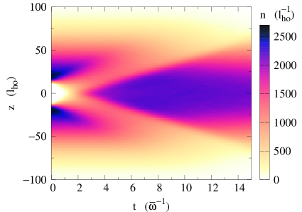
Figure 1: 1d density profile $n(z,t)$ as function of position $z$ (vertical axis) and time $t$ (horizontal axis) after the removal of the barrier.

we show the 1d density profile $n(z,t)$ as a function of $z$ and $t$. After $t\sim\bar{\omega}^{-1}\sim 1$ ms, the two clouds start to touch each other, and at $t\sim 2$ ms the density starts to develop a peak at $z=0$, as in the experiment Joseph2011 . At later times, the peak expands and the density inside becomes flat. There is a clear separation between the central region with high density and the outer part with lower density. As a function of time, this step moves outwards and was identified with a shock front.

The box-like shape of the high-density region can be better seen in the upper panels of Fig. 2

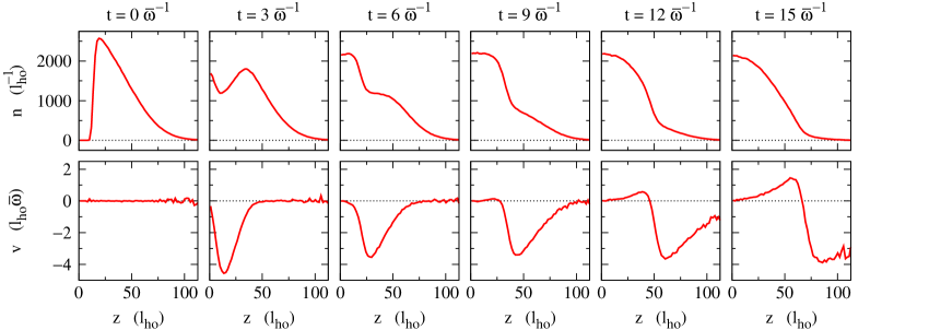
Figure 2: Snapshots of the density profile $n(z)$ (top) and velocity profile $v(z)$ (bottom) at different times $t$ after the removal of the barrier. Only positive $z$ values are shown, since $n(-z)=n(z)$ and $v(-z)=-v(z)$ for symmetry reasons.

which show snapshots of the density profile, especially at $t=6\,\bar{\omega}^{-1}$ and $t=9\,\bar{\omega}^{-1}$. In the lower panels of Fig. 2, we show the velocity $v$. Although the central region with high density and low velocity is clearly separated from the outer part with lower density which continues to fall inwards ($v<0$), $n$ and $v$ are of course not really discontinuous, but the shock front has a finite width. Let us mention that the numerical noise of average quantities per particle in the low-density region corresponds to statistical fluctuations due to the test-particle method and that the smooth aspect observed otherwise has been obtained by averaging over several runs with different microscopic initializations. More specifically, the Boltzmann results shown in this work correspond to averages over 48 runs, each involving $5\times 10^{4}$ test particles.

In LABEL:Joseph2011, this violent two-cloud collision with shock wave formation was studied within a 1d superfluid hydrodynamic (i.e., zero-temperature) model. In order to obtain the finite width of the shock front, the Euler equation was extended to include a viscous force, and the viscosity was determined by fitting the experimental density profile. However, the viscous force should in principle be accompanied by dissipation, i.e., heating, in order to conserve the total energy. In our case, since we start already from a finite temperature, it is clear that for the hydrodynamic description one has to solve three coupled equations, corresponding to the conservation of particle number, momentum, and energy. It turns out that not only the viscosity but also the heat conductivity is crucial if one wants to reproduce the Boltzmann results, see Sec. V.

IV Momentum anisotropy in the shock front

It was already pointed out long time ago Mott-Smith1951 that hydrodynamics, even with viscosity and heat conductivity, is not applicable in the shock front. To see this in the present case, we compare the following moments of the distribution function

$$\varepsilon_{\text{kin},x}(z)=\frac{1}{2m}\langle p_{x}^{2}\rangle\,,$$ (9)

$$\varepsilon_{\text{pot},x}(z)=\frac{m\omega_{\perp}^{2}}{2}\langle x^{2}\rangle\,,$$ (10)

$$\varepsilon_{\text{kin},z}(z)=\frac{1}{2m}(\langle p_{z}^{2}\rangle-\langle p_{z}\rangle^{2})\,,$$ (11)

where the averages $\langle\cdots\rangle$ are defined as in Eq. (8). Because of axial symmetry, we have of course $\varepsilon_{\text{kin},y}=\varepsilon_{\text{kin},x}$ and $\varepsilon_{\text{pot},y}=\varepsilon_{\text{pot},x}$ (with $\varepsilon_{\text{kin},y}$ and $\varepsilon_{\text{pot},y}$ defined analogously to $\varepsilon_{\text{kin},x}$ and $\varepsilon_{\text{pot},x}$). In the 1d hydrodynamic model, one would assume a local equilibrium in the sense that $\varepsilon_{\text{kin},x}=\varepsilon_{\text{pot},x}=\varepsilon_{\text{kin},z}=\varepsilon/5$ with $\varepsilon$ the internal energy per particle in the local fluid rest frame. In a classical gas, $\varepsilon_{\text{kin},x}$ and $\varepsilon_{\text{kin},z}$ can be identified with “anisotropic temperatures” $T_{\perp}$ and $T_{z}$ in transverse and longitudinal directions, respectively.

In Fig. 3

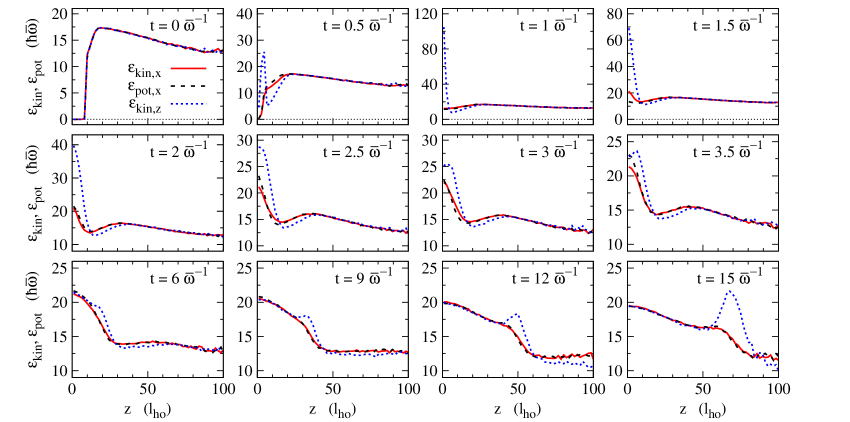
Figure 3: Moments $\varepsilon_{\text{kin},x}(z)$ (red solid lines), $\varepsilon_{\text{pot},x}(z)$ (black dashes) and $\varepsilon_{\text{kin},z}(z)$ (blue dots) as functions of $z$ (calculated in 200 bins) at different times $t$ after the removal of the barrier.

we show $\varepsilon_{\text{kin},x}(z)$, $\varepsilon_{\text{pot},x}(z)$, and $\varepsilon_{\text{kin},z}(z)$ for different times after the removal of the barrier. One can clearly see that the equipartition in the transverse direction, $\varepsilon_{\text{kin},x}=\varepsilon_{\text{pot},x}$, is very well fulfilled, except for a fast oscillation of $\varepsilon_{\text{kin},x}$ against $\varepsilon_{\text{pot},x}$ in the beginning of the collision. This is, however, not the case for the longitudinal direction. One clearly sees that $\varepsilon_{\text{kin},z}>\varepsilon_{\text{kin},x}$ in the region of the shock front, even at large times when the shock front reaches the low-density region. Far away from the shock, the gas is in local equilibrium and one finds $\varepsilon_{\text{kin},x}=\varepsilon_{\text{kin},z}$. Far outside, the gas becomes classical with $\varepsilon_{\text{kin},i}=T/2$ (the initial temperature is $T=25.3\,\hbar\bar{\omega}$). In the center, the relation between $\varepsilon_{\text{kin},i}$ and the temperature is more complicated because the gas is degenerate and $\varepsilon_{\text{kin},i}$ is dominated by Fermi motion.

In fact, the result $\varepsilon_{\text{kin},z}>\varepsilon_{\text{kin},x}$ can be intuitively understood: particles entering the zone of the shock from the dilute region need to undergo a couple of collisions before their distribution corresponds to the equilibrium one of the dense region. Because of the different $\langle p_{z}\rangle$ in the two regions, the variance of $p_{z}$ in the transition region is obviously larger than the variance of $p_{x}$.

Within this picture, the ansatz for a bimodal momentum distribution used in LABEL:Mott-Smith1951 looks very natural: there, the momentum distribution in the shock front is written as a superposition of equilibrium distributions corresponding to the mean velocities and temperatures on both sides of the shock. Recent high-precision numerical calculations confirm this picture, see e.g. LABEL:Malkov2015.

However, when we analysed our momentum distribution in the shock front we did not find any bimodality. This may have two reasons: first, our gas is not classical but degenerate, which leads to a substantial broadening of the momentum distribution, and second, the shock we are studying is not very violent. Therefore, one could maybe describe the anisotropy of the momentum distribution in the shock front within the framework of the so-called “anisotropic fluid dynamics” Bluhm2015 .

V 1d hydrodynamic model

In the original experimental paper Joseph2011 the shape of the shock front was used to extract an effective viscosity parameter. Therefore, it is interesting to study how far one can get with viscous hydrodynamics in spite of the anisotropy of the momentum distribution in the shock front discussed in the preceding section. In our case, we assume that the system is in the normal-fluid phase at finite temperature, which makes the hydrodynamic description somewhat more complicated and requires to include also the heat conductivity.

Starting from the usual (3d) hydrodynamic equations (cf. LABEL:Landau6, Eqs. (15.5) and (49.2)), integrating over $x$ and $y$, assuming that the system remains always in equilibrium in the transverse direction [i.e., $T_{\text{3d}}(\bm{\mathrm{r}})=T(z)$ and $\mu_{\text{3d}}(\bm{\mathrm{r}})=\mu(z)-m\omega_{\perp}^{2}r_{\perp}^{2}/2m$] and neglecting the contribution of the transverse components of the fluid velocity $\bm{\mathrm{v}}_{\text{3d}}$ to the energy, one obtains the following 1d hydrodynamic equations:

$$\dot{n}=-(nv)^{\prime}\,,$$ (12)

$$(nv)^{\!\mbox{$\cdot$}}=-\Big{(}nv^{2}+\frac{P}{m}\Big{)}^{\prime}+n\frac{F}{m}+\frac{4}{3m}(\eta v^{\prime})^{\prime}\,,$$ (13)

$$(nE)^{\!\mbox{$\cdot$}}=-(nvE+vP)^{\prime}+nvF+\Big{(}\frac{4}{3}\eta vv^{\prime}+\kappa T^{\prime}\Big{)}^{\prime}\,,$$ (14)

describing the conservation of particle number, momentum, and energy. In these equations, $E=\varepsilon+\tfrac{1}{2}mv^{2}$ is the total energy per particle, $P$ is the pressure integrated over $x$ and $y$, $F=-m\omega_{z}^{2}z$ is the $z$ component of the external force, and $\kappa$ and $\eta$ are respectively the heat conductivity and shear viscosity integrated over $x$ and $y$ (in the presence of a non-vanishing bulk viscosity $\zeta$, one would have to replace $\tfrac{4}{3}\eta$ by $\tfrac{4}{3}\eta+\zeta$). Derivatives are denoted as $\dot{v}=\partial v/\partial t$ and $v^{\prime}=\partial v/\partial z$ etc.

To close this system of equations, it is necessary to express $P$, $T$, $\eta$ and $\kappa$ in terms of $n$ and $\varepsilon$. Since we neglect the mean field, we consider the equation of state (EOS) of an ideal gas, $P=(\gamma-1)n\varepsilon$, with $\gamma=\tfrac{7}{5}$ as in a gas of diatomic molecules because the internal energy $\varepsilon$ includes five degrees of freedom ($\varepsilon_{\text{kin},x}$, $\varepsilon_{\text{kin},y}$, $\varepsilon_{\text{kin},z}$, $\varepsilon_{\text{pot},x}$, $\varepsilon_{\text{pot},y}$). To find $T$, it is convenient to write $n$ and $P$ as functions of $\mu$ and $T$ in the form $n=A\,T^{5/2}F_{3/2}(\mu/T)$ and $n\varepsilon=A\,T^{7/2}F_{5/2}(\mu/T)$, with the abbreviation $A=4\sqrt{2m}/(3\pi\omega_{\perp}^{2})$ and the integrals of the Fermi function $F_{\alpha}(x)=\int_{0}^{\infty}\!dt\,t^{\alpha}/(e^{t-x}+1)$. The functions $F_{\alpha}$ and their inverse functions $X_{\alpha}$ [i.e., $X_{\alpha}(F_{\alpha}(x))=x$] can be very efficiently approximated Antia1993 and then $T$ is obtained by solving numerically the equation $X_{5/2}(n\varepsilon/(A\,T^{7/2}))=X_{3/2}(n/(A\,T^{5/2}))$. For $\eta$, we follow Joseph2011 and assume that $\eta=\tilde{\eta}n$ with some constant $\tilde{\eta}$, although this choice cannot easily be justified. Similarly, we also assume that $\kappa=\tilde{\kappa}n/m$. The dimensionless (for $\hbar=k_{B}=1$) proportionality constants $\tilde{\eta}$ and $\tilde{\kappa}$ are fitted to give reasonable agreement with the Boltzmann results. In the notation of LABEL:Joseph2011, our $\tilde{\eta}$ corresponds to $\tfrac{3}{4}m\nu$. For completeness, we recall that in LABEL:Joseph2011 a value of $\tilde{\eta}=7.5$ was obtained at (almost) zero temperature.

Although Eqs. (12)–(14) can formally be obtained by integrating the 3d hydrodynamic equations over $x$ and $y$, the equipartition of the energy among the five internal degrees of freedom observed in the Boltzmann results seems to indicate that the range of validity of the 1d equations is actually larger than that of the 3d equations which must fail at large $x$ and $y$ where no collisions take place.

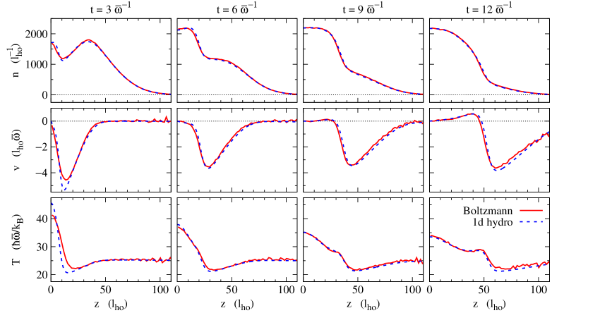
Figure 4: Comparison between 1d hydrodynamic (blue dashes) and Boltzmann (red solid lines) results for the density $n$, the velocity $v$, and the temperature $T$ in trap units (from top to bottom) at four different times $t=3,6,9$ and $12\,\bar{\omega}^{-1}$. The dimensionless viscosity and heat conductivity parameters are $\tilde{\eta}=9$ and $\tilde{\kappa}=34$. The Boltzmann results for the temperature were obtained using the EOS of the ideal Fermi gas with harmonic radial confinement (see text) with the Boltzmann results for $n$ and $\varepsilon$ as input.

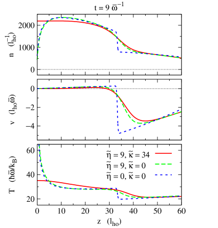
Figure 5: Results of 1d hydrodynamics for the density $n$, the velocity $v$, and the temperature $T$ in trap units (from top to bottom) at $t=9\,\bar{\omega}^{-1}$. Red solid line: results obtained with $\tilde{\eta}=9$ and $\tilde{\kappa}=34$; green long dashes: $\tilde{\eta}=9$ but no heat conductivity; blue short dashes: no viscosity and no heat conductivity.

The numerical solution of Eqs. (12)–(14) is nontrivial. Because of the instabilities of standard methods in the case of shock waves, dedicated methods have been developed. Here we use the code “hydro1d” Zingale-hydro1d based on Riemann solvers Toro which we have extended to include the external force in axial direction due to the trap potential, the above mentioned EOS of the Fermi gas with harmonic radial confinement, and the viscosity $\eta$ and heat conductivity $\kappa$. The viscous and heat conduction terms, like the external force, were implemented as source terms added to the equations in conservative form (similar to the implementation of gravity in the original hydro1d code).

Except at small times ($t\lesssim 5\,\bar{\omega}^{-1}$), an excellent agreement between hydrodynamic and Boltzmann results can be achieved with $\tilde{\eta}=9$ and $\tilde{\kappa}=34$ as can be seen in Fig. 4, showing various snapshots for the density $n$, velocity $v$ and temperature $T$ profiles. When determining these values, we have assumed that the ratio $\eta/\kappa$ is approximately given by the ratio of $\eta_{\text{3d}}/\kappa_{\text{3d}}=\tfrac{4}{15}m$ obtained in kinetic theory Bruun2007 ; Braby2010 .

The importance of the heat conductivity becomes clear from Fig. 5, where we focus on a single snapshot, and compare different hydrodynamics results for the profiles of $n$, $v$ and $T$. There, the red solid curves represent the full results with viscosity and heat conduction, while the long green dashes were obtained without heat conduction and the short blue dashes without heat conduction and viscosity. While the viscosity alone, without heat conduction, is sufficient to smoothen the discontinuity across the shock front, it does not remove the unrealistic hole in the density profile at $z=0$. This hole is related to the temperature peak at $z=0$ which is created during the initial stage of the collision. The hole in $n$ and the peak in $T$ lead to a pressure that is practically constant around $z=0$, so that there is no acceleration of matter. Hence, without heat conduction, the peak in $T$ remains there forever and so does the hole in $n$. But notice that, even with $\tilde{\kappa}=34$ the temperature peak melts more slowly within 1d hydrodynamics than within Boltzmann (cf. Fig. 4, $t=3\,\bar{\omega}^{-1}$).

The sharp shock front in the case $\tilde{\eta}=\tilde{\kappa}=0$ allows us to extract quantitatively some information which is difficult to obtain from the smooth shock front in the realistic case. In particular, one can read off the speed $v_{s}$ of the shock front from $v_{s}=(v_{1}n_{1}-v_{2}n_{2})/(n_{1}-n_{2})$ where $v_{i}$ and $n_{i}$ are the velocities and densities on both sides of the discontinuity. Using this, one can define the Mach numbers $\text{Ma}_{i}=|v_{i}-v_{s}|/c_{i}$ where $c_{i}$ is the speed of sound on side $i$ of the discontinuity. The upstream Mach number (i.e., the one on the right-hand side of the discontinuity if one looks at $z>0$), which quantifies the strength of the shock, is $\text{Ma}\approx 2.6$ at $t=2\,\bar{\omega}^{-1}$. It decreases rapidly to $\text{Ma}\approx 1.6$ at $t=6\,\bar{\omega}^{-1}$. At $t\gtrsim 12\,\bar{\omega}^{-1}$, when the shock reaches the low-density region, it starts to increase again.

VI Conclusions

In this paper, we applied the Boltzmann equation within the test-particle method to the description of the dynamics of a violent collision between two ultracold clouds as described in LABEL:Joseph2011. Within our approach, it is not possible to simulate exactly the experimental conditions since the initial temperature in the experiment is such that the system is superfluid. We thus focused on the dynamics of the normal phase at higher temperature. In that respect we have described in detail the formation and propagation of the shock front as observed in LABEL:Joseph2011. A direct comparison with a 1d hydrodynamic approach clearly indicates that the extraction of a viscosity parameter directly from a fit of the density profile is probably doubtful and that the inclusion of a thermal conductivity is unavoidable if one wants to get closer to the Boltzmann simulation and prevent from unphysical behavior.

In this paper, we were mainly interested in the comparison between Boltzmann and hydrodynamic calculations. Therefore we consistently used in the Boltzmann calculation the propagation in the trap potential without mean field, and in the hydrodynamic calculation the equation of state of the ideal Fermi gas. For a quantitative comparison with recent experiments done at finite temperatures Roof2018 , it will be necessary to go beyond these approximations, i.e., to include the mean field in the Boltzmann calculation and the equation of state of the unitary Fermi gas Ku2012 in the hydrodynamic calculation. As already mentioned in Sec. II, also the in-medium modification of the cross section in the collision term should be taken into account. We are currently working on these extensions of the present study.

As a perspective for future work, the emergence of the effective 1d hydrodynamic behavior needs to be better understood from the microscopic point of view. In particular, the effective 1d viscosity and heat conductivity cannot be obtained by integrating the corresponding 3d quantities over $r_{\perp}$ and should be derived from a transport theory. Since even in the shock front the momentum anisotropy seems to be moderate, it may be also possible to achieve this goal within the recently developed anisotropic fluid dynamics Bluhm2015 . Furthermore, to address also the situation of the gas being, at least partly, in the superfluid phase, a more sophisticated theory would be needed that combines the hydrodynamic description of the superfluid with a transport equation for the normal-fluid component.

References

- (1) J. A. Joseph, J. E. Thomas, M. Kulkarni, A. G. Abanov, Phys. Rev. Lett. 106, 150401 (2011).
- (2) R. Becker, Z. Phys. 8, 321 (1922).
- (3) H.-M. Mott-Smith, Phys. Rev. 82, 885 (1951).
- (4) W. Scheid, H. Müller, and W. Greiner, Phys. Rev. Lett. 32, 741 (1973).
- (5) P. Danielewicz, Nucl. Phys. A 314, 465 (1979).
- (6) L. Salasnich, Europhys. Lett. 96, 40007 (2011).
- (7) F. Ancilotto, L. Salasnich, F. Toigo, Phys. Rev. A 85, 063612 (2012).
- (8) W. Wen, T. Shui, Y. Shan, and C. Zhu, J. Phys. B: At. Mol. Opt. Phys. 48, 175301 (2015).
- (9) N. K. Lowman, M. A. Hoefer, Phys. Rev. A 88, 013605 (2013).
- (10) A. Bulgac, Y.-L Luo, K. J. Roche, Phys. Rev. Lett. 108, 150401 (2012).
- (11) T. Lepers, D. Davesne, S. Chiacchiera, M. Urban, Phys. Rev. A 82, 023609 (2010).
- (12) P.-A. Pantel, D. Davesne, M. Urban, Phys. Rev. A, 91, 013627 (2015).
- (13) E. M. Lifshitz and L. P. Pitaevskii, Physical Kinetics, Landau-Lifshitz Course of Theoretical Physics, vol. 10 (Pergamon, Oxford, 1980).
- (14) S. Chiacchiera, T. Lepers, D. Davesne, and M. Urban Phys. Rev. A 79, 033613 (2009).
- (15) S. Riedl, E. R. Sanchez Guajardo, C. Kohstall, A. Altmeyer, M. J. Wright, J. H. Denschlag, R. Grimm, G. M. Bruun, and H. Smith, Phys. Rev. A 78, 053609 (2008).
- (16) S. Chiacchiera, T. Lepers, D. Davesne, and M. Urban, Phys. Rev. A 84, 043634 (2011).
- (17) C. Cao, E. Elliott, J. Joseph, H. Wu, J. Petricka, T. Schäfer, and J. E. Thomas, Science 331, 58 (2011).
- (18) E. Elliott, J. A. Joseph, and J. E. Thomas, Phys. Rev. Lett. 112, 040405 (2014).
- (19) O. Goulko, F. Chevy, and C. Lobo, New J. Phys. 14, 073036 (2012).
- (20) O. Goulko, F. Chevy, and C. Lobo, Phys. Rev. A 84, 051605 (2011).
- (21) E. A. Malkov, Ye. A. Bondar, A. A. Kokhancik, O. Poleshkin, M. S. Ivsnov, Shock Waves 25, 387 (2015).
- (22) M. Bluhm and T. Schäfer, Phys. Rev. A 92, 043602 (2015).
- (23) L. D. Landau and E. M. Lifshitz, Fluid Mechanics, Course of Theoretical Physics, vol. 6, 2nd ed. (Pergamon, Oxford 1987).
- (24) H. M. Antia, Astrophys. J. Suppl. 84, 101 (1993).
- (25) M. Zingale, http://zingale.github.io/hydro1d/
- (26) E. F. Toro, Riemann Solvers and Numerical Methods for Fluid Dynamics: A Practical Introduction, 3rd ed. (Springer, Berlin 2009).
- (27) G. M. Bruun and H. Smith, Phys. Rev. A 75, 043612 (2007).
- (28) M. Braby, J. Chao, and T. Schäfer, Phys. Rev. A 82, 033619 (2010).
- (29) S. Roof and J. E. Thomas, private communication.
- (30) M. J. H. Ku, A. T. Sommer, L. W. Cheuk, and M. W. Zwierlein, Science 335, 563 (2012).