Abstract

We prove that deciding if a diagram of the unknot can be untangled using at most $k$ Riedemeister moves (where $k$ is part of the input) is NP-hard. We also prove that several natural questions regarding links in the $3$-sphere are NP-hard, including detecting whether a link contains a trivial sublink with $n$ components, computing the unlinking number of a link, and computing a variety of link invariants related to four-dimensional topology (such as the $4$-ball Euler characteristic, the slicing number, and the $4$-dimensional clasp number).

1 Introduction

Unknot recognition via Reidemeister moves.

The unknot recognition problem asks whether a given knot is the unknot. Decidability of the unknot recognition problem was established by Haken [Hak61], and since then several other algorithms were constructed (see for example the survey of Lackenby [Lac17a]).

One can ask, naively, if one can decide if a given knot diagram represents the unknot simply by untangling the diagram: trying various Reidemeister moves until there are no more crossings. A first issue is that one might need to increase the number of crossings at some point in this untangling: examples of “hard unknots” witnessing this necessity can be found in Kaufman and Lambropoulou [KL14] . The problem then, obviously, is knowing when to stop: if we have not been able to untangle the diagram using so many moves, is the knot in question necessarily knotted or should we keep on trying?

In [HL01], Hass and Lagarias gave an explicit (albeit rather large) bound on the number of Reidemeister moves needed to untangle a diagram of the unknot. Lackenby [Lac15] improved the bound to polynomial thus showing that the unknot recognition problem is in NP (this was previously proved in [HLP99]). The unknot recognition problem is also in co-NP [Lac16] (assuming the Generalized Riemann Hypothesis, this was previously shown by Kuperberg [Kup14]). Thus if the unknot recognition problem were NP-complete (or co-NP-complete) we would have that NP and co-NP coincide which is commonly believed not to be the case. This suggests that the unknot recognition problem is not NP-hard.

It is therefore natural to ask if there is a way to use Reidemeister moves leading to a better solution than a generic brute-force search. Our main result suggests that there may be serious difficulties in such an approach: given a 3-SAT instance $\Phi$ we construct an unknot diagram and a number $k$, so that the diagram can be untangled using at most $k$ Reidemeister moves if and only if $\Phi$ is satisfiable. Hence any algorithm that can calculate the minimal number of Reidemeister moves needed to untangle unknot diagrams will be robust enough to tackle any problem in NP.

The main result of this paper is:

Theorem 1.

Given an unknot diagram $D$ and an integer $k$, deciding if $D$ can be untangled using at most $k$ Reidemeister moves is NP-complete.

Lackenby [Lac15] proved that the problem above is in NP, and therefore we only need to show NP-hardness.

For the reduction in the proof of Theorem 1 we have to construct arbitrarily large diagrams of the unknot. The difficulty in the proof is to establish tools powerful enough to provide useful lower bounds on the minimal number of Reidemeister moves needed to untangle these diagrams. For instance, the algebraic methods of Hass and Nowik [HN10] are not strong enough for our reduction. It is also quite easy to modify the construction and give more easily lower bounds on the number of Reidemeister moves needed to untangle unlinks if one allows the use of arbitrarily many components of diagrams with constant size, but those techniques too cannot be used for Theorem 1. We develop the necessary tools in Section 4.

Computational problems for links.

Our approach for proving Theorem 1 partially builds on techniques to encode satisfiability instances using Hopf links and Borromean rings, that we previously used in [dMRST18] (though the technical details are very different). With these techniques, we also show that a variety of link invariants are NP-hard to compute.

Precisely, we prove:

Theorem 2.

Given a link diagram $L$ and an integer $k$, the following problems are NP-hard:

1. deciding whether $L$ admits a trivial unlink with $k$ components as a sublink.

2. deciding whether an intermediate invariant has value $k$ on $L$,

3. deciding whether $\chi_{4}(L)=0$,

4. deciding whether $L$ admits a smoothly slice sublink with $k$ components.

We refer to Definition 12 for the definitions of $\chi_{4}(L)$, the $4$-ball Euler characteristic, and of intermediate invariants. These are broadly related to the topology of the $4$-ball, and include the unlinking number, the ribbon number, the slicing number, the concordance unlinking number, the concordance ribbon number, the concordance slicing number, and the $4$-dimensional clasp number. See, for example, [Shi74] for a discussion of many intermediate invariants.

Related complexity results.

The complexity of computational problems pertaining to knots and links is quite poorly understood. In particular, only very few computational lower bounds are known, and as far as we know, almost none concern classical knots (i.e., knots embedded in ${S}^{3}$): apart from our Theorem 1, the only other such hardness proof we know of [KS, Sam18] concerns counting coloring invariants (i.e., representations of the fundamental group) of knots. More lower bounds are known for classical links. Lackenby [Lac17b] showed that determining if a link is a sublink of another one is NP-hard. Our results strengthen this by showing that even finding an $n$-component unlink as a sublink is already NP-hard. Agol, Hass and Thurston [AHT06] showed that computing the genus of a knot in a $3$-manifold is NP-hard, and Lackenby [Lac17b] showed that computing the Thurston complexity of a link in ${S}^{3}$ is also NP-hard. Our results complement this by showing that the $4$-dimensional version of this problem is also NP-hard.

Regarding upper bounds, the current state of knowledge is only slightly better. While, as we mentioned before, it is now known that the unknot recognition problem is in $\textbf{NP}\cap$ co-NP, many natural link invariants are not even known to be decidable. In particular, this is the case for all the invariants for which we prove NP-hardness, except for the problem of finding the maximal number of components of a link that form an unlink, which is in NP (see Theorem 4).

Shortly before we finished our manuscript, Koenig and Tsvietkova posted a preprint [KT18] that also shows that certain computational problems on links are NP-hard, with some overlap with the results obtained in this paper (the trivial sublink problem and the unlinking number). They also show NP-hardness of computing the number of Reidemeister moves for getting between two diagrams of the unlink, but their construction does not untangle the diagram and requires arbitrarily many components. Theorem 1 of the current paper is stronger and answers Question 17 of [KT18].

Organization.

This paper is organized as follows. After some preliminaries in Section 2, we start by proving the hardness of the trivial sublink problem in Part I because it is very simple and provides a good introduction for our other reductions. We then proceed to prove Theorem 1 in Part II and the hardness of the unlinking number and the other invariants in Part III. The three parts are independent and the reader can read any one part alone.

2 Preliminaries

Notation.

Most of the notation we use is standard. By knot we mean a tame piecewise linear embedding of the circle $S^{1}$ into the $3$-sphere $S^{3}$. By link we mean a tame, piecewise linear embedding of the disjoint union of any finite number of copies of $S^{1}$. We use interval notation for natural numbers, for example, $[3,5]$ means $\{3,4,5\}$; we use $[12]$ to indicate $[1,12]$. We assume basic familiarity with computational complexity and knot theory, and refer to basic textbooks such as Arora and Barak [AB09] for the former and Rolfsen [Rol90] for the latter.

Diagram of a knot or a link.

All the computational problems that we study in this paper take as input the diagram of a knot or a link, which we define here.

A diagram of a knot is a piecewise linear map $D\colon S^{1}\to{\mathbb{R}}^{2}$ in general position; for such a map, every point in ${\mathbb{R}}^{2}$ has at most two preimages, and there are finitely many points in ${\mathbb{R}}^{2}$ with exactly two preimages (called crossing). Locally at crossing two arcs cross each other transversely, and the diagram contains the information of which arc passes ‘over’ and which ‘under’. This we usually depict by interrupting the arc that passes under. (A diagram usually arises as a composition of a (piecewise linear) knot $\kappa\colon S^{1}\to{\mathbb{R}}^{3}$ and a generic projection $\pi\colon{\mathbb{R}}^{3}\to{\mathbb{R}}^{2}$ which also induces ‘over’ and ‘under’ information.) We usually identify a diagram $D$ with its image in ${\mathbb{R}}^{2}$ together with the information about underpasses/overpasses at crossings; see, for example, Figure 3, ignoring the notation on the picture. Diagrams are considered up-to isotopy.

Similarly, a diagram of a link is a piecewise linear map $D\colon\coprod S^{1}\to{\mathbb{R}}^{2}$ in general position, where $\coprod$ denotes a disjoint union of a finite number of circles $S^{1}$, and with the same additional information at the crossings.

By an arc in the diagram $D$ we mean a set $D(\alpha)$ where $\alpha$ is an arc in $S^{1}$ (i.e., a subset of $S^{1}$ homeomorphic to the closed interval).

The size of a knot or a link diagram is its number of crossings plus number of components of the link. Up to a constant factor, this complexity exactly describes the complexity of encoding the combinatorial information contained in a knot or link diagram.

$3$-satisfiability.

A formula in conjunctive normal form in variables $x_{1},\dots,x_{n}$ is a Boolean formula of the form $c_{1}\wedge c_{2}\wedge\cdots\wedge c_{m}$ where each $c_{i}$ is a clause, that is, a formula of the form $(\ell_{1}\vee\ell_{2}\vee\cdots\vee\ell_{k})$ where each $\ell_{j}$ is a literal, that is, a variable $x_{t}$ or its negation $\neg x_{t}$. A formula $\Phi$ is satisfiable if there is an assignment to the variables (each variable is assigned $\operatorname{TRUE}$ or $\operatorname{FALSE}$) such that $\Phi$ evaluates to $\operatorname{TRUE}$ in the given assignment.

A 3-SAT problem is the well-known NP-hard problem. On input there is a formula $\Phi$ in conjunctive normal form such that every clause contains exactly three variables; see, e.g., [Pap94, Proposition 9.2].

Part I Trivial sublink

Informally, the trivial sublink problem asks, given a link $L$ and a positive integer $n$, whether $L$ admits the $n$-component unlink as a sublink. We define:

Definition 3 (The Trivial Sublink Problem).

An unlink, or a trivial link, is a link in $S^{3}$ whose components bound disjointly embedded disks. A trivial sublink of a link $L$ is an unlink formed by a subset of the components of $L$. The trivial sublink problem asks, given a link $L$ and a positive integer $n$, whether $L$ admits an $n$ component trivial sublink.

Theorem 4.

The trivial sublink problem is NP-complete.

Note that Theorem 4 is just a slight extension of Theorem 2(a), claiming also NP-membership. The essential part is NP-hardness.

Proof.

It follows from Hass, Lagarias, and Pippenger [HLP99] that deciding if a link is trivial is in NP. By adding to their certificate a collection of $n$ components of $L$ we obtain a certificate for the trivial sublink problem, showing that it is in NP (NP-membership of the trivial sublink problem was also established, using completely different techniques, by Lachenby [Lac15]). Thus all we need to show is that the problem is NP-hard. We will show this by reducing 3-SAT to the trivial sublink problem.

Given a 3-SAT instance $\Phi$, with $n$ variables (say $x_{1},\dots,x_{n}$) and $m$ clauses, we construct a diagram $D_{\Phi}$ as follows (see Figure 1):

Figure 1: $D_{\Phi}$ for $\Phi=(x\vee y\vee z)\wedge(x\vee\neg y\vee t)$)

we first mark $n+m$ disjoint disks in the plane. In each of the first $n$ disks we draw a diagram of the Hopf link, marking the components in the $i$th disk as $\kappa_{x_{i}}$ and $\kappa_{\neg x_{i}}$. In the remaining $m$ disks we draw diagrams of the Borromean rings and label them according to the clauses of $\Phi$. We now band each component of the Borromean rings to the Hopf link component with the same label. Whenever two bands cross we have one move over the other (with no “weaving”); we assume, as we may, that no two bands cross twice. It is easy to see that this can be done in polynomial time. The diagram we obtain is $D_{\Phi}$ and the link it represents is denoted $L_{\Phi}$ (note that $L_{\Phi}$ has exactly $2n$ components). We complete the proof by showing that $L_{\Phi}$ admits an $n$-component trivial sublink exactly when $\Phi$ is satisfiable.

Claim 4.1.

If $\Phi$ is satisfiable then $L_{\Phi}$ admits an $n$-component trivial sublink.

Given a satisfying assignment we remove from $L_{\Phi}$ the components that correspond to satisfied literals, that is, if $x_{i}=\operatorname{TRUE}$ we remove $\kappa_{x_{i}}$ from $L_{\Phi}$ and if $x_{i}=\operatorname{FALSE}$ we remove $\kappa_{\neg x_{i}}$ from $L_{\Phi}$. We claim that the remaining $n$ components form an unlink. To see this, first note that since the assignment is satisfying, from each copy of the Borromean rings at least one component was removed. Therefore the rings fall apart and (since we did not allow “weaving”) the diagram obtained retracts into the first $n$ disks. In each of these disks we had, originally, a copy of the Hopf link; by construction exactly one component was removed. This shows that the link obtained is indeed the $n$-component unlink; Claim 4.1 follows.

Claim 4.2.

If $L_{\Phi}$ admits an $n$-component trivial sublink, then $\Phi$ is satisfiable.

Suppose that $L_{\Phi}$ admits an $n$-component trivial sublink $\mathcal{U}$. Since $\mathcal{U}$ itself does not admit the Hopf link as a sublink, for each $i$, at most one of $\kappa_{x_{i}}$ and $\kappa_{\neg x_{i}}$ is in $\mathcal{U}$. Since $\mathcal{U}$ has $n$ components we see that exactly one of $\kappa_{x_{i}}$ and $\kappa_{\neg x_{i}}$ is in $\mathcal{U}$. If $\kappa_{x_{i}}$ is in $\mathcal{U}$ we set $x_{i}=\operatorname{FALSE}$ and if $\kappa_{\neg x_{i}}$ is in $\mathcal{U}$ we set $x_{i}=\operatorname{TRUE}$. Now since $\mathcal{U}$ does not admit the Borromean rings as a sublink, from each copy of the Borromean rings at least one component is not in $\mathcal{U}$. It follows that in each clause of $\Phi$ at least one literal is satisfied, that is, the assignment satisfies $\Phi$; Claim 4.2 follows.

This completes the proof of Theorem 4. ∎

Part II The number of Reidemeister moves for untangling

3 A restricted form of the satisfiability problem

For the proof of Theorem 1, we will need a slightly restricted form of the 3-SAT problem given by lemma below.

Lemma 5.

Deciding whether a formula $\Phi$ in conjunctive normal form is satisfiable is NP-hard even if we assume the following conditions on $\Phi$.

• Each clause contains exactly three literals.

• No clause contains both $x$ and $\neg x$ for some variable $x$.

• Each pair of literals $\{\ell_{1},\ell_{2}\}$ occurs in at most one clause.

Proof.

The first condition says that we consider the 3-SAT problem. Any clause violating the second condition can be removed from the formula without affecting satisfiability of the formula as such clause is always satisfied. Therefore, it is sufficient to provide a recipe to build in polynomial time a formula $\Phi$ satisfying the three conditions above out of a formula $\Phi^{\prime}$ satisfying only the first two conditions.

First, we consider an auxiliary formula

$$\Psi=\Psi(t,a,b,c)=(t\vee a\vee\neg b)\wedge(t\vee b\vee\neg c)\wedge(t\vee c\vee\neg a)\wedge(a\vee b\vee c)\wedge(\neg a\vee\neg b\vee\neg c).$$

We observe that for any satisfying assignment of $\Psi$ we get that $t$ is assigned $\operatorname{TRUE}$. Indeed, if $t$ were assigned $\operatorname{FALSE}$ then $(t\vee a\vee\neg b)\wedge(t\vee b\vee\neg c)\wedge(t\vee c\vee\neg a)$ translates as $(b\Rightarrow a)\wedge(c\Rightarrow b)\wedge(a\Rightarrow c)$, that is all $a$, $b$, and $c$ are equivalent. However, then $(a\vee b\vee c)\wedge(\neg a\vee\neg b\vee\neg c)$ cannot be satisfied.

On the other hand, we also observe that there is a satisfying assignment for $\Psi$ where $t$ is assigned $\operatorname{TRUE}$ and, for example, it is sufficient to assign $a$ with $\operatorname{TRUE}$, $b$ with $\operatorname{FALSE}$ and $c$ arbitrarily.

Now we return to the formula $\Phi^{\prime}$ discussed above. Suppose there exists a pair literals $\ell_{1}$ and $\ell_{2}$ contained in two clauses of $\Phi^{\prime}$, say $(\ell_{1}\vee\ell_{2}\vee\ell_{3})$ and $(\ell_{1}\vee\ell_{2}\vee\ell_{4})$. We replace them with

$$(\ell_{1}\vee\ell_{2}\vee x)\wedge(\ell_{3}\vee\neg x\vee\neg t_{1})\wedge(\ell_{4}\vee\neg x\vee\neg t_{2})\wedge\Psi(t_{1},a_{1},b_{1},c_{1})\wedge\Psi(t_{2},a_{2},b_{2},c_{2}),$$

where $x,t_{1},t_{2},a_{1},a_{2},b_{1},b_{2},c_{1},$ and $c_{2}$ are newly added variables, obtaining a new formula $\Phi^{\prime\prime}$. We aim to show that $\Phi^{\prime\prime}$ is satisfiable if and only if $\Phi^{\prime}$ is satisfiable.

Let us first assume that $\Phi^{\prime}$ is satisfiable and fix a satisfying assignment. If $\ell_{1}\vee\ell_{2}$ is $\operatorname{TRUE}$ in this assignment, then we may extend it to variables of $\Phi^{\prime\prime}$ by setting $x$ to $\operatorname{FALSE}$, $t_{1}$ and $t_{2}$ to $\operatorname{TRUE}$ and $a_{1},\dots,c_{2}$ so that $\Psi(t_{1},a_{1},b_{1},c_{1})\wedge\Psi(t_{2},a_{2},b_{2},c_{2})$ is satisfied. If $\ell_{1}\vee\ell_{2}$ is $\operatorname{FALSE}$ in the assignment for $\Phi^{\prime}$, then $\ell_{3}$ and $\ell_{4}$ must be assigned $\operatorname{TRUE}$. Then we may extend by setting $x$ to $\operatorname{TRUE}$ and $t_{1},t_{2},a_{1},\dots,c_{2}$ as before.

Now let us assume that $\Phi^{\prime\prime}$ is satisfiable. Then $t_{1}$ and $t_{2}$ are set to $\operatorname{TRUE}$ due to the properties of $\Psi$. If $x$ is $\operatorname{TRUE}$, then both $\ell_{3}$ and $\ell_{4}$ must be true and the restriction of the assignment on $\Phi^{\prime\prime}$ to the variables of $\Phi^{\prime}$ is therefore a satisfying assignment for $\Phi^{\prime}$. Similarly, if $x$ is $\operatorname{FALSE}$, then $\ell_{1}\vee\ell_{2}$ must be true and the restriction is again a satisfying assignment for $\Phi^{\prime}$.

We also observe that in $\Phi^{\prime\prime}$ we have reduced the number of clauses containing the literals $\ell_{1}$ and $\ell_{2}$ simultaneously, and for any other pair of literals we do not increase the number of clauses containing that pair. Therefore, after a polynomial number of steps, when always adding new variables, we arrive at a desired formula $\Phi$ satisfying all three conditions. ∎

4 The defect

Reidemeister moves.

Reidemeister moves are local modifications of a diagram depicted in Figure 2 (the labels at the crossings in a $\rm{III}$ move will be used only later on). We distinguish the $\rm{I}$ move (left), the $\rm{II}$ move (middle) and the $\rm{III}$ move (right). The first two moves affect the number of crossings, thus we further distinguish the $\rm{I}^{-}$ and the $\rm{II}^{-}$ moves which reduce the number of crossings from the $\rm{I}^{+}$ and the $\rm{II}^{+}$ moves which increase the number of crossings.

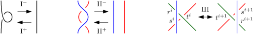
Figure 2: Reidemeister moves

The number of Reidemeister moves for untangling a knot.

A diagram of an unknot is untangled if it does not contain any crossings. The untangled diagram is denoted by $U$. Given a diagram $D$ of an unknot, an untangling of $D$ is a sequence $\mathbf{D}=(D^{0},\dots,D^{k})$ where $D^{0}=D$, $D^{k}=U$ (recall that diagrams are only considered up to isotopy) and $D^{i}$ is obtained from $D^{i-1}$ by a single Reidemeister move. The number of Reidemeister moves in $\mathbf{D}$ is denoted by $\operatorname{rm}(\mathbf{D})$, that is, $\operatorname{rm}(\mathbf{D})=k$. We also define $\operatorname{rm}(D):=\min\operatorname{rm}(\mathbf{D})$ where the minimum is taken over all untanglings $\mathbf{D}$ of $D$.

The defect.

Let us denote by $\operatorname{cross}(D)$ the number of crossings in $D$. Then the defect of an untangling $\mathbf{D}$ is defined by the formula

$$\operatorname{def}(\mathbf{D}):=2\operatorname{rm}(\mathbf{D})-\operatorname{cross}(D).$$

The defect of a diagram $D$ is defined as $\operatorname{def}(D):=2\operatorname{rm}(D)-\operatorname{cross}(D)$. Equivalently, $\operatorname{def}(D)=\min\operatorname{def}(\mathbf{D})$ where the minimum is taken over all untanglings $\mathbf{D}$ of $D$.

The defect is a convenient way to reparametrize the number of Reidemeister moves due to the following observation.

Observation 6.

For any diagram $D$ of the unknot and any untangling $\mathbf{D}$ of $D$ we have $\operatorname{def}(\mathbf{D})\geq 0$. Equality holds if and only if $\mathbf{D}$ uses only $\rm{II}^{-}$ moves.

Proof.

Every Reidemeister move in $\mathbf{D}=(D^{0},\dots,D^{k})$ removes at most two crossings and the $\rm{II}^{-}$ move is the only move that removes exactly two crossings. Therefore, the number of crossings in $D=D^{0}$ is at most $2k$ and equality holds if and only if every move is a $\rm{II}^{-}$ move. ∎

Crossings contributing to the defect.

Let $\mathbf{D}=(D^{0},\dots,D^{k})$ be an untangling of a diagram $D=D^{0}$ of an unknot.

Given a crossing $r^{i}$ in $D^{i}$, for $0\leq i\leq k-1$, it may vanish by the move transforming $D^{i}$ into $D^{i+1}$ if this is a $\rm{I}^{-}$ or a $\rm{II}^{-}$ move affecting the crossing. In all other cases it survives and we denote by $r^{i+1}$ the corresponding crossing in $D_{i+1}$. Note that in the case of a $\rm{III}$ move there are three crossings affected by the move and three crossings afterwards. Both before and after, each crossing is the unique intersection between a pair of the three arcs of the knot that appear in this portion of the diagram. So we may say that these three crossings survive the move though they change their actual geometric positions (they swap the order in which they occur along each of the three arcs); see Figure 2.

With a slight abuse of terminology, by a crossing in $\mathbf{D}$ we mean a maximal sequence $\mathbf{r}=(r^{a},r^{a+1},\dots,r^{b})$ such that $r^{i+1}$ is the crossing in $D^{i+1}$ corresponding to $r^{i}$ in $D^{i}$ for any $i\in[a,b-1]$. By maximality we mean, that $r^{b}$ vanishes after the $(b+1)$st move and either $a=0$ or $r^{a}$ is introduced by the $a$th Reidemeister move (which must be a $\rm{I}^{+}$ or $\rm{II}^{+}$ move).

An initial crossing is a crossing $\mathbf{r}=(r^{0},r^{1},\dots,r^{b})$ in $\mathbf{D}$. Initial crossings in $\mathbf{D}$ are in one-to-one correspondence with crossings in $D=D^{0}$. For simplicity of notation, $r^{0}$ is also denoted $r$ (as a crossing in $D$).

A Reidemeister $\rm{II}^{-}$ move in $\mathbf{D}$ is economical, if both crossings removed by this move are initial crossings; otherwise, it is wasteful.

Let $m_{3}(\mathbf{r})$ be the number of $\rm{III}$ moves affecting a crossing $\mathbf{r}$. The weight of an initial crossing $\mathbf{r}$ is defined in the following way.

$$w(\mathbf{r})=\frac{2}{3}m_{3}(\mathbf{r})+\left\{\begin{array}[]{ll}0&\mbox{if $\mathbf{r}$ vanishes by an economical $\rm{II}^{-}$ move};\\ 1&\mbox{if $\mathbf{r}$ vanishes by a $\rm{I}^{-}$ move};\\ 2&\mbox{if $\mathbf{r}$ vanishes by a wasteful $\rm{II}^{-}$ move}.\\ \end{array}\right.$$

For later purposes, we also define $w(r):=w(\mathbf{r})$ and $w(R):=\sum_{r\in R}w(r)$ for a subset $R$ of the set of all crossings in $D$.

Lemma 7.

Let $\mathbf{D}$ be an untangling of a diagram $D$. Then

$$\operatorname{def}(\mathbf{D})\geq\sum\limits_{\mathbf{r}}w(\mathbf{r}),$$

where the sum is over all initial crossings $\mathbf{r}$ of $\mathbf{D}$.

Proof.

In the proof we use the discharging technique, common in graph theory.

Let us put charges on crossings in $\mathbf{D}$ and on Reidemeister moves used in $\mathbf{D}$. The initial charge will be

• on each Reidemeister move;

• on each initial crossing; and

• on each non-initial crossing.

We remark that the sum of the initial charges equals to $\operatorname{def}(\mathbf{D})$ by the definition of the defect.

Now we start redistributing the charge according to the rules described below. The aim is that, after the redistribution, the charge on each initial crossing will be at least $w(\mathbf{r})$ and it will be at least $0$ on non-initial crossings and on Reidemeister moves. This will prove the lemma, as the sum of the charges after the redistribution is still equal to the defect, whereas it will be at least the sum of the weights of initial crossings.

We apply the following rules for the redistribution of the charge.

• Every $\rm{I}^{+}$ move sends charge $2$ to the (non-initial) crossing it creates.

• Every $\rm{I}^{-}$ move sends charge $2$ to the crossing it removes.

• Every $\rm{II}^{+}$ move sends charge $1$ to each of the two (non-initial) crossings it creates.

• Every economical $\rm{II}^{-}$ move sends charge $1$ to each of the two (initial) crossings it removes.

• Every wasteful $\rm{II}^{-}$ move that removes exactly one initial crossing sends charge $3$ to this initial crossing.

• Every $\rm{III}$ move sends $\frac{2}{3}$ to every crossing it affects.

• Every non-initial crossing which is removed by a wasteful $\rm{II}^{-}$ move sends charge $1$ to this move.

Now it is routine to check that the desired conditions are satisfied, which we now explain.

Every move has charge at least $0$: The initial charge on moves is $2$. The rules are set up so that every move distributes charge at most $2$ with exception of the rule (R5). However, in this case, the wasteful $\rm{II}^{-}$ move that removes exactly one initial crossing from (R5) gets $1$ charge from rule (R7).

Every non-initial crossing has charge at least $0$: The initial charge is $0$. The only rule that depletes the charge is (R7); however in such case, the charge is replenished by (R1) or (R3).

Every initial crossing $\mathbf{r}$ has charge equal at least $w(\mathbf{r})$: The initial charge is $-1$. First we observe that (R6) sends the charge $\frac{2}{3}m_{3}(\mathbf{r})$ to $\mathbf{r}$. If $\mathbf{r}$ vanishes by an economical $\rm{II}^{-}$ move, it gets additional charge $1$ by (R4). If $\mathbf{r}$ vanishes by a $\rm{I}^{-}$ move, it gets additional charge $2$ by (R2). Finally, if $\mathbf{r}$ vanishes by a wasteful $\rm{II}^{-}$ move then this move removes exactly one initial crossing, namely $\mathbf{r}$. Therefore $\mathbf{r}$ gets an additional charge $3$ by (R5). ∎

We will also need a variant for a previous lemma where we get equality, if we use the $\rm{I}^{-}$ and $\rm{II}^{-}$ moves only.

Lemma 8.

Let $\mathbf{D}$ be an untangling of a digram $D$ which uses the $\rm{I}^{-}$ and $\rm{II}^{-}$ moves only. Then

$$\operatorname{def}(\mathbf{D})=\sum\limits_{\mathbf{r}}w(\mathbf{r})=\hbox{ number of $\rm{I}^{-}$ moves},$$

where the sum is over all initial crossings $\mathbf{r}$ of $\mathbf{D}$.

Proof.

Let $k_{1}$ be the number of initial crossings removed by a $\rm{I}^{-}$ move and $k_{2}$ the number of initial crossings removed by a $\rm{II}^{-}$ move. Then $\operatorname{rm}(\mathbf{D})=k_{1}+k_{2}/2$ and from the definition of the defect we get $\operatorname{def}(\mathbf{D})=2(k_{1}+k_{2}/2)-(k_{1}+k_{2})=k_{1}$. It follows directly the definition of the weight that $k_{1}=\sum\limits_{\mathbf{r}}w(\mathbf{r})$. ∎

Twins and the preimage of a bigon.

Let $\mathbf{r}$ be an initial crossing in an untangling $\mathbf{D}=(D^{0},\dots,D^{k})$ removed by an economical $\rm{II}^{-}$ move. The twin of $\mathbf{r}$, denoted by $t(\mathbf{r})$ is the other crossing in $\mathbf{D}$ removed by the same $\rm{II}^{-}$ move. Note that $t(\mathbf{r})$ is also an initial crossing (because of the economical move). We also get $t(t(\mathbf{r}))=\mathbf{r}$. If $\mathbf{r}=(r^{0},r^{1},\dots,r^{b})$, then we also extend the definition of a twin to $D^{i}$ in such a way that $t(r^{i})$ is uniquely defined by $t(\mathbf{r})=(t(r^{0}),\dots,t(r^{b}))$. In particular, we will often use a twin $t(r)$ of a crossing $r=r^{0}$ in $D$ (if it exists).

Furthermore, the crossings $r^{b}$ and $t(r^{b})$ in $D^{b}$ form a bigon that is removed by the forthcoming $\rm{II}^{-}$ move. Let $\alpha^{b}(r)$ and $\beta^{b}(r)$ be the two arcs of the bigon (with endpoints $r^{b}$ and $t(r^{b})$) so that $\alpha^{b}(r)$ is the arc that, after extending slightly, overpasses the crossings $r^{b}$ and $t(r^{b})$ whereas a slight extension of $\beta^{b}(r)$ underpasses these crossings. (The reader may remember this as $\alpha$ is ‘above’ and $\beta$ is ‘below’.) Now we can inductively define arcs $\alpha^{i}(r)$ and $\beta^{i}(r)$ for $i\in[0,b-1]$ so that $\alpha^{i}(r)$ and $\beta^{i}(r)$ are the unique arcs between $r^{i}$ and $t(r^{i})$ which are transformed to (already defined) $\alpha^{i+1}(r)$ and $\beta^{i+1}(r)$ by the $i$th Reidemeister move. We also set $\alpha(r)=\alpha^{0}(r)$ and $\beta(r)=\beta^{0}(r)$. Intuitively, $\alpha(r)$ and $\beta(r)$ form a preimage of the bigon removed by the $(b+1)$st move and they are called the preimage arcs between $r$ and $t(r)$.

Close neighbors.

Let $R$ be a subset of the set of crossings in $D$. Let $r$ and $s$ be any two crossings in $D$ (not necessarily in $R$) and let $c$ be a non-negative integer. We say that $r$ and $s$ are $c$-close neighbors with respect to $R$ if $r$ and $s$ can be connected by two arcs $\alpha$ and $\beta$ such that

• $\alpha$ enters $r$ and $s$ as an overpass;

• $\beta$ enters $r$ and $s$ as an underpass;

• $\alpha$ and $\beta$ may have self-crossings; however, neither $r$ nor $s$ is in the interior of $\alpha$ or $\beta$; and

• $\alpha$ and $\beta$ together contain at most $c$ crossings from $R$ in their interiors. (If there is a crossing in the interior of both $\alpha$ and $\beta$, this crossing is counted only once.)

Lemma 9.

Let $R$ be a subset of the set of crossings in $D$, let $c\in\{0,1,2,3\}$. Let $r$ be the crossing in $R$ which is the first of the crossings in $R$ removed by an economical $\rm{II}^{-}$ move (we allow a draw). If $w(R)\leq c$, then $r$ and its twin $t(r)$ are $c$-close neighbors with respect to $R$.

Proof.

Let $\alpha(r)$ and $\beta(r)$ be the preimage arcs between $r$ and $t(r)$. We want to verify that they satisfy the properties of the arcs from the definition of the close neighbors. The first two properties follow immediately from the definition of preimage arcs.

Next, we want to check that neither $r$ nor $t(r)$ is the interior of $\alpha(r)$ or $\beta(r)$. For contradiction, let us assume that this not the case. For example, suppose that $r$ also lies in the interior of $\alpha(r)$. Let $\mathbf{r}=(r,r^{1},\dots,r^{b})$ be the initial crossing corresponding to $r$. The $(b+1)$st Reidemeister move in $\mathbf{D}$ removes $\mathbf{r}$. Any preceding Reidemeister move either does not affect $\mathbf{r}$ at all, or it is a $\rm{III}$ move swapping the crossing with other crossings. In any case, it preserves the self-crossing of $\alpha(r)$ at $\mathbf{r}$. However, this contradicts the fact that $\alpha(r^{b})$ is an arc of a bigon removed by the $(b+1)$st move.

In order to check the last property, let us assume that, for contradiction, $\alpha(r)$ and $\beta(r)$ together contain at least $c+1$ crossings from $R(x)$ in their interiors. These crossings have to be removed from the arcs $\alpha(r)$ and $\beta(r)$ until we reach $\alpha(r^{b})$ and $\beta(r^{b})$. They cannot be removed by an economical $\rm{II}^{-}$ move as $r$ is the first crossing from $R(x)$ removed by such a move. Thus they have to be removed from the arcs either by a $\rm{I}^{-}$ move, a wasteful $\rm{II}$ move or a $\rm{III}$ move (by swapping with $r$ or $t(r)$). This contradicts $w(x)\leq c$. Indeed, if only $\rm{I}^{-}$ and $\rm{II}^{-}$ moves are used, we get a total weight at least $c+1$ on the crossings; if at least one $\rm{III}$ move is used, we get a weight at least $(c+1)\cdot\frac{2}{3}$ on the crossings and an additional $\frac{2}{3}$ on $r$ or $t(r)$. This is in total more than $c$ as $c\leq 3$. ∎

5 The reduction

Let $\Phi$ be a formula in conjunctive normal form satisfying the conditions stated in Lemma 5 and let $n$ be the number of variables. Our aim is to build a diagram $D(\Phi)$ by a polynomial-time algorithm such that $\operatorname{def}(D(\Phi))\leq n$ if and only if $\Phi$ is satisfiable.

The variable gadget.

First we describe the variable gadget. For every variable $x$ we consider the diagram depicted at Figure 3 and we denote it $V(x)$.

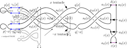
Figure 3: The variable gadget $V(x)$.

The gadget contains $17$ crossings $p[x],p[\neg x],q[x],q[\neg x]$, $r(x)$ and $s_{i}(x)$ for $i\in[12]$. The variable gadget also contains six distinguished arcs $\gamma_{i}[x]$ and $\gamma_{i}[\neg x]$ for $i\in[2]$, $\delta(x)$ and $\varepsilon(x)$ and six distinguished auxiliary points $a_{1}(x),\dots,a_{6}(x)$ which will be useful later on in order to describe how the variable gadget is used in the diagram $D(\Phi)$.

We also call the arc between $a_{1}(x)$ and $a_{2}(x)$ which contains $\gamma_{1}[x]$ and $\gamma_{2}[x]$ the $x$ tentacle, and similarly, the arc between $a_{2}(x)$ and $a_{3}(x)$ which contains $\gamma_{1}[\neg x]$ and $\gamma_{2}[\neg x]$ is the $\neg x$ tentacle. Informally, a satisfying assignment to $\Phi$ will correspond to the choice whether we will decide to remove first the loop at $p[x]$ by a $\rm{I}^{-}$ move and simplify the $x$ tentacle or whether we remove first the loop at $p[\neg x]$ and remove the $\neg x$ tentacle in the final construction of $D(\Phi)$.

We also remark that in the notation, we use square brackets for objects that come in pairs and will correspond to a choice of literal $\ell\in\{x,\neg x\}$. This regards $p[\ell]$, $q[\ell]$, $\gamma_{1}[\ell]$ and $\gamma_{2}[\ell]$ whereas we use parentheses for the remaining objects.

The clause gadget.

Given a clause $c=(\ell_{1}\vee\ell_{2}\vee\ell_{3})$ in $\Phi$, the clause gadget is depicted at Figure 4. The construction is based on the Borromean rings. It contains three pairs of arcs (distinguished by color) and with a slight abuse of notation, we refer to each of the three pairs of arcs as a “ring”. Note that each ring has four pendent endpoints (or leaves) as in the picture. Each ring corresponds to one of the literals $\ell_{1}$, $\ell_{2}$, and $\ell_{3}$.

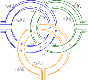
Figure 4: The clause gadget for clause $c=(\ell_{1}\vee\ell_{2}\vee\ell_{3})$.

A blueprint for the construction.

Now we build a blueprint for the construction of $D(\Phi)$. Let $x_{1},\dots,x_{n}$ be the variables of $\Phi$ and let $c_{1},\dots,c_{m}$ be the clauses of $\Phi$.

For each clause $c_{j}=(\ell_{1}\vee\ell_{2}\vee\ell_{3})$ we take a copy of the graph $K_{1,3}$ (also known as the star with three leaves). We label the vertices of degree $1$ of such a $K_{1,3}$ by the literals $\ell_{1}$, $\ell_{2}$, and $\ell_{3}$. Now we draw these stars into the plane sorted along a horizontal line; see Figure 5.

Figure 5: A blueprint for the construction of $D(\Phi)$.

Next for each literal $\ell\in\{x_{1},\dots,x_{n},\neg x_{1},\dots,\neg x_{n}\}$ we draw a piecewise linear segment containing all vertices labelled with that literal according to the following rules (follow Figure 5).

• The segments start on the right of the graphs $K_{1,3}$ in the top down order $x_{1},\neg x_{1}$, $x_{2},\neg x_{2}$, $\dots,x_{n},\neg x_{n}$.

• They continue to the left while we permute them to the order $x_{1},\dots,x_{n}$, $\neg x_{1},\dots,\neg x_{n}$. We also require that $x_{1},\dots,x_{n}$ occur above the graphs $K_{1,3}$ and $\neg x_{1},\dots,\neg x_{n}$ occur below these graphs (everything is still on the right of the graphs).

• Next, for each literal $\ell$ the segment for $\ell$ continues to the left while it makes a ‘detour’ to each vertex $v$ labelled $\ell$. If $v$ is not the leftmost vertex labelled $\ell$, then the detour is performed by a ‘finger’ of two parallel lines. We require that the finger avoids the graphs $K_{1,3}$ except of the vertex $v$. If $v$ is the leftmost vertex labelled $\ell$, then we perform only a half of the finger so that $v$ becomes the endpoint of the segment.

Note that the segments often intersect each other; however, for any $i\in[n]$ the segments for $x_{i}$ and $\neg x_{i}$ do not intersect (using the assumption that no clause contains both $x_{i}$ and $\neg x_{i}$).

The final diagram.

Finally, we explain how to build the diagram $D(\Phi)$ from the blueprint above.

Step I (four parallel segments): We replace each segment for a literal $\ell$ with four parallel segments; see Figure 6. The outer two will correspond to the arc $\gamma_{1}[\ell]$ from the variable gadget and the inner two will correspond to $\gamma_{2}[\ell]$; compare with Figure 3.

Figure 6: Step I: Replacing segments.

Step II (clause gadgets): We replace each copy of $K_{1,3}$ by a clause gadget for the corresponding clause $c$; see Figure 7. Now we aim to describe how is the clause gadget connected to the quadruples of parallel segments obtained in Step I. Let $v$ be a degree $1$ vertex of the $K_{1,3}$ we are just replacing. Let $\ell$ be the literal which is the label of this vertex. Then $c$ may or may not be the leftmost clause containing a vertex labelled $\ell$.

Figure 7: Step II: Replacing the $K_{1,3}$.

If $c$ is the leftmost clause containing a vertex labelled $\ell$, then there are four parallel segments for $\ell$ with pendent endpoints (close to the original position of $v$) obtained in Step I. We connect them to the pendent endpoints of the clause gadget (on the ring for $\ell$); see $\neg x_{2}$ and $x_{4}$ at Figure 7. Note also that at this moment the two $\gamma_{1}[\ell]$ arcs introduced in Step I merge as well as the two $\gamma_{2}[\ell]$ arcs merge.

If $c$ is not the leftmost clause labelled $\ell$ then there are four parallel segments passing close to $v$ (forming a tip of a finger from the blueprint). We disconnect the two segments closest to the tip of the finger and connect them to the pendent endpoints of the clause gadget (on the ring for $\ell$); see $\neg x_{1}$ at Figure 7.

Step III (resolving crossings): If two segments in the blueprint, corresponding to literals $\ell$ and $\ell^{\prime}$ have a crossing, Step I blows up such a crossing into $16$ crossing of corresponding quadruples. We resolve overpasses/underpasses at all these crossings in the same way. That is, one quadruple overpasses the second quadruple at all $16$ crossings; see Figure 8.

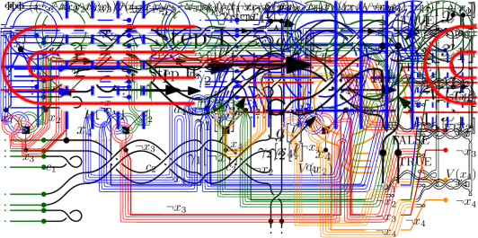
Figure 8: Step III: Resolving crossings.

However, we require one additional condition on the choice of overpasses/underpasses. If $\ell$ and $\ell^{\prime}$ appear simultaneously in some clause $c$ we have $8$ crossings on the rings for $\ell$ and $\ell^{\prime}$ in the clause gadget for $c$. We can assume that the ring of $\ell$ passes over the ring of $\ell^{\prime}$ at all these crossings (otherwise we swap $\ell$ and $\ell^{\prime}$). Then for the $16$ crossings on segments for $\ell$ and $\ell^{\prime}$ we pick the other option, that is we want that the $\gamma_{1}[\ell]$ and $\gamma_{2}[\ell]$ arcs underpass the $\gamma_{1}[\ell^{\prime}]$ and $\gamma_{2}[\ell^{\prime}]$ arcs at these crossings. This is a globally consistent choice because we assume that there is at most one clause containing both $\ell$ and $\ell^{\prime}$, this is the third condition in the statement of Lemma 5.

STEP IV (the variable gadgets): Now, for every variable $x_{i}$, the segments $\gamma_{1}[x_{i}],\gamma_{2}[x_{i}],\gamma_{1}[\neg x_{i}]$ and $\gamma_{2}[\neg x_{i}]$ do not intersect each other. We extend them to a variable gadget as on Figure 9. Namely, to the bottom left endpoints of $\gamma_{1}[x_{i}],\gamma_{2}[x_{i}],\gamma_{1}[\neg x_{i}]$ and $\gamma_{2}[\neg x_{i}]$ we glue the parts of the variable gadget containing the crossings $p[x_{i}]$ and $p[\neg x_{i}]$ and to the top left endpoints of $\gamma_{1}[x_{i}],\gamma_{2}[x_{i}],\gamma_{1}[\neg x_{i}]$ and $\gamma_{2}[\neg x_{i}]$ we glue the remainder of the variable gadget. At this moment, we obtain a diagram of a link, where each link component has a diagram isotopic to the diagram on Figure 3.

Figure 9: Step IV: Adding the variable gadgets.

STEP V (interconnecting the variable gadgets): Finally, we form a connected sum of individual components. Namely, for every $i\in[n-1]$ we perform the knot sum along the arcs $\delta(x_{i})$ and $\varepsilon(x_{i+1})$ by removing them and identifying $a_{4}(x_{i})$ with $a_{1}(x_{i+1})$ and $a_{6}(x_{i})$ with $a_{5}(x_{i+1})$ as on Figure 10. The arcs $\delta(x_{1})$ and $\varepsilon(x_{n})$ remain untouched. This way we obtain the desired diagram $D(\Phi)$; see Figure 11.

Figure 10: Step V: Interconnecting the variable gadgets.

Figure 11: The final construction for the formula $\Phi=(x_{1}\vee x_{2}\vee x_{3})\wedge(\neg x_{1}\vee x_{2}\vee\neg x_{3})\wedge(\neg x_{1}\vee\neg x_{2}\vee x_{4})\wedge(x_{1}\vee\neg x_{3}\vee\neg x_{4})$. For simplicity of the picture, we do not visualize how the crossings are resolved in Step III. (Unfortunately, we cannot avoid tiny pictures of gadgets.)

The core of the NP-hardness reduction is the following theorem.

Theorem 10.

Let $\Phi$ be a formula in conjunctive normal form satisfying the conditions in the statement of Lemma 5. Then $\operatorname{def}(D(\Phi))\leq n$ if and only if $\Phi$ is satisfiable.

Theorem 1 immediately follows from Theorem 10 and Lemma 5:

Proof of Theorem 1 modulo Theorem 10.

Due to the definition of the defect, the minimum number of Reidemeister moves required to untangle $D$ equals $\frac{1}{2}(\operatorname{def}(D(\Phi))-\operatorname{cross}(D(\Phi))$. Therefore, setting $k=\frac{1}{2}(n+\operatorname{cross}(D(\Phi))$, Theorem 10 gives that $D(\Phi)$ can be untangled with at most $k$ moves if and only if $\Phi$ is satisfiable. This gives the required NP-hardness via Lemma 5. (Note also, that $D(\Phi)$ and $k$ can be constructed in polynomial time in the size of $\Phi$.) ∎

The remainder of this section is devoted to the proof of Theorem 10.

5.1 Satisfiable implies small defect

The purpose of this subsection is to prove the ‘if’ implication of Theorem 10. That is we are given a satisfiable $\Phi$ and we aim to show that $\operatorname{def}(D(\Phi))\leq n$.

Let us consider a satisfying assignment. For any literal $\ell$ assigned $\operatorname{TRUE}$ we first remove the loop at the $p[\ell]$ vertex in the variable gadget (see Figure 3) by a $\rm{I}^{-}$ move. This way, we use one $\rm{I}^{-}$ move on each variable gadget, that is $n$ such moves. Next we aim to show that it is possible to finish the untangling of the diagram by $\rm{II}^{-}$ moves only. As soon as we do this, we get an untangling with defect $n$ by Lemma 8 which will finish the proof.

Thus it remains to finish the untangling with $\rm{II}^{-}$ moves only. We again pick $\ell$ assigned $\operatorname{TRUE}$ and we start shrinking the $\ell$ tentacle by $\rm{II}^{-}$ moves. This way we completely shrink $\gamma_{1}[\ell]$ and $\gamma_{2}[\ell]$ as due to the construction as all arcs that meet $\gamma_{1}[\ell]$ simultaneously meet $\gamma_{2}[\ell]$ and vice versa. See Figure 12 for the initial $\rm{I}^{-}$ move and a few initial $\rm{II}^{-}$ moves. Furthermore we can continue shrinking the $\ell$ tentacle until we get a loop next to the $q[\ell]$ vertex; see Figure 13.

Figure 12: Initial simplifications.

Figure 13: The $\ell$ tentacle was shrunk to a loop next to $q[\ell]$. In this example we have $\ell=\neg x_{i}$.

We continue the same process for every literal $\ell$ assigned $\operatorname{TRUE}$. In the intermediate steps, some of the other arcs meeting $\gamma_{1}[\ell]$ and $\gamma_{2}[\ell]$ might have already been removed. However, it is still possible to simplify the $\ell$ tentacle as before. See Figure 14 for the result after shrinking all tentacles assigned $\operatorname{TRUE}$.

Figure 14: Simplifying the tentacles according to a satisfying assignment $x_{1}=x_{2}=x_{4}=\operatorname{TRUE}$, $x_{3}=\operatorname{FALSE}$.

Because we assume that we started with a satisfying assignment, in each clause gadget at least one ring among the three Borromean rings disappears. Consequently, if there are two remaining rings in some clause gadget, then they can be pulled apart from each other by $\rm{II}^{-}$ moves as on Figure 15.

Figure 15: Untangling two rings in the clause gadget via $\rm{II}^{-}$ moves.

After this step, for each $\ell$ assigned $\operatorname{TRUE}$, the $\gamma_{1}[\neg\ell]$ and $\gamma_{2}[\neg\ell]$ form ‘fingers’ of four parallel curves. These fingers can be further simplified by $\rm{II}^{-}$ moves so that any crossings among different fingers are removed; see Figure 16. For each variable gadget $V(x)$ we get one of the two possible pictures at Figure 17 left. Both of them simplify to the picture on the right by three further $\rm{II}^{-}$ moves.

Figure 16: Simplifying $\gamma_{1}[\neg\ell]$ and $\gamma_{2}[\neg\ell]$ via $\rm{II}^{-}$ moves. First, we untangle the inner (horizontal) ‘finger’ and then we untangle the outer (horizontal) ‘finger’.

Figure 17: Results of the simplifications on the previous picture on the level of variable gadgets.

Finally, we recall how are the variable gadgets interconnected (compare the right picture at Figure 17 with Figure 10). Then it is easy to remove all remaining $2n$ crossings by $\rm{II}^{-}$ moves gradually from top to bottom. This finishes the proof of the ‘if’ part of Theorem 10.

5.2 Small defect implies satisfiable

The purpose of this subsection is to prove the ‘only if’ part of the statement of Theorem 10. Recall that this means that we assume $\operatorname{def}(D(\Phi))\leq n$ and we want to deduce that $\Phi$ is satisfiable. (Along the way we will actually also deduce that $\operatorname{def}(D(\Phi))=n$.) In this subsection, we heavily use the terminology introduced in Section 4.

Let $\mathbf{D}=(D^{0},\dots,D^{k})$ be an untangling of $D$ with $\operatorname{def}(\mathbf{D})\leq n$. For a variable $x$ let $R(x)=\{p[x],p[\neg x],q[x],q[\neg x],s_{1}(x),\dots,s_{12}(x)\}$ be the set of $16$ out of the $17$ self-crossings in the variable gadget $V(x)$ (we leave out $r(x)$) and let the weight of $x$, denoted by $w(x)$, be the sum of weights of the crossings in $R(x)$.

Our first aim is to analyze the first economical $\rm{II}^{-}$ move that removes some of the crossings in $R(x)$, using Lemma 9.

Claim 10.1.

Let $x$ be a variable with $w(x)\leq 1$. Let $r$ be the crossing in $R(x)$ which is the first of the crossings in $R(x)$ removed by an economical $\rm{II}^{-}$ move (we allow a draw). Then one of the following cases holds

1. $\{r,t(r)\}=\{s_{1}(x),s_{2}(x)\}$, $w(p[x])=w(x)=1$ and $p[x]$ is removed by a $\rm{I}^{-}$ move prior to removing $r$ and $t(r)$.

2. $\{r,t(r)\}=\{s_{1}(x),s_{3}(x)\}$, $w(p[\neg x])=w(x)=1$ and $p[\neg x]$ is removed by a $\rm{I}^{-}$ move prior to removing $r$ and $t(r)$.

Before we start the proof, we remark that the condition $w(x)\leq 1$ implies that there are (at least $15$) crossings in $R(x)$ removed by economical $\rm{II}^{-}$ moves. In particular, $r$ in the statement always exists.

Proof.

First, we need to identify the possible pairs $\{r,t(r)\}$ where $r\in R(x)$. Such pairs are found by a case analysis, using Lemma 9 with $c=1$ and $R=R(x)$.

The general strategy is the following. For each element of $R(x)$ we consider whether it may be $r$. We analyze possible arcs $\alpha$ and $\beta$ from the definition of $c$-close neighbors.

There are two directions in which $\alpha$ may emanate from $r$. For each direction we allow up to one internal crossing from $R(x)$ on $\alpha$, getting a candidate position for $t(r)$ (even if $\alpha$ passes through other variable gadgets we count only the crossings from $R(x)$). We immediately disregard the cases when $\alpha$ passes through $r$ again (this is not allowed by the third item of the definition of close neighbors). We also emphasize that we are interested only in the cases when $\alpha$ enters the candidate $t(r)$ as an overpass.

Next, we refocus on $\beta$; again there are two possible directions and we again identify possible the possible position of $t(r)$ (this time entered as an underpass).

Finally, we compare the lists of candidate positions for $t(r)$ obtained for $\alpha$ and for $\beta$; it must be possible to obtain $t(r)$ in both ways.

The candidate positions of $t(r)$ as an endpoint of $\alpha$ and as an endpoint of $\beta$ are summarized in Table 1; and they can be easily found with the aid of Figure 3. Note that it follows from the construction of $D(\Phi)$ that $\delta(x)$ and $\varepsilon(x)$ are (usually) not in $D(\Phi)$. For considerations in the table, we denote by $\delta^{\prime}(x)$ the arc in $D(\Phi)$ between the points $a_{1}(x)$ and $a_{5}(x)$ which avoids $r(x)$ (equivalently, any other crossing in $V(x)$). Similarly, we let $\varepsilon^{\prime}(x)$ denote the arc in $D(\Phi)$ between the points $a_{4}(x)$ and $a_{6}(x)$ which avoids $r(x)$. The table also misses values for $r=s_{9}(x)$ which requires a separate analysis.

In order to avoid any ambiguity, we explain how the first row of the table is obtained, considering the case $r=p[x]$ (follow Figure 3):

Choice of $r$	$t(r)$ in $\alpha$	$t(r)$ in $\beta$	Overlap
$p[x]$	$\gamma_{2}[x]$	$\gamma_{1}[x],s_{2}(x),s_{4}(x)$	$\emptyset$
$p[\neg x]$	$\gamma_{2}[\neg x],s_{3}(x),s_{4}(x)$	$\gamma_{1}[\neg x]$	$\emptyset$
$s_{1}(x)$	$\gamma_{1}[\neg x],\gamma_{2}[\neg x],s_{3}(x),s_{2}(x)$	$\gamma_{2}[x],\gamma_{1}[x],s_{2}(x),s_{3}(x)$	$s_{2}(x),s_{3}(x)$
$s_{2}(x)$	$s_{1}(x),\gamma_{1}[\neg x]$	$\gamma_{1}[x],p[x],\gamma_{2}[x],s_{1}(x),s_{4}(x)$	$s_{1}(x)$
$s_{3}(x)$	$\gamma_{2}[\neg x],p[\neg x],\gamma_{1}[\neg x],s_{1}(x),s_{4}(x)$	$s_{1}(x),\gamma_{2}[x]$	$s_{1}(x)$
$s_{4}(x)$	$s_{3}(x),\gamma_{2}[\neg x],p[\neg x]$	$s_{2}(x),\gamma_{1}[x],p[x]$	$\emptyset$
$s_{5}(x)$	$s_{6}(x)$	$s_{7}(x)$	$\emptyset$
$s_{6}(x)$	$s_{5}(x)$	$s_{8}(x),q[\neg x]$	$\emptyset$
$s_{7}(x)$	$s_{8}(x),q[x]$	$s_{5}(x)$	$\emptyset$
$s_{8}(x)$	$s_{7}(x),q[x]$	$s_{6}(x),q[\neg x]$	$\emptyset$
$q[x]$	$s_{7}(x),s_{8}(x)$	$s_{9}(x),s_{11}(x)$	$\emptyset$
$q[\neg x]$	$s_{9}(x),s_{10}(x)$	$s_{6}(x),s_{8}(x)$	$\emptyset$
$s_{9}(x)$	separate analysis
$s_{10}(x)$	$s_{9}(x),q[\neg x],\delta^{\prime}(x),r(x),\varepsilon^{\prime}(x)$	$s_{12}(x)$	$\emptyset$
$s_{11}(x)$	$s_{12}(x)$	$s_{9}(x),q[x],r(x),\varepsilon^{\prime}(x),\delta^{\prime}(x)$	$\emptyset$
$s_{12}(x)$	$s_{11}(x)$	$s_{10}(x)$	$\emptyset$

Table 1: Possible positions for $t(r)$ depending on $r$ in Claim 10.1.

We know that $\alpha$ may emanate to the left or to the right. Emanating to the left is immediately ruled out as we reach $p[x]$ again in the next crossing. Emanating to the right allows $t(r)$ to be some crossing on $\gamma_{2}[x]$ or seemingly it may be $s_{1}(x)$ or $s_{3}(x)$; however $s_{1}(x)$ and $s_{3}(x)$ are entered by $\alpha$ as an underpass, so they cannot be $t(r)$. Therefore the only option, from the point of view of $\alpha$, is that $t(r)$ belongs to $\gamma_{2}[x]$, as marked in Table 1. Similarly when focusing on $\beta$, emanating to the left is immediately ruled out whereas emanating to the right allows $t(r)$ to belong $\gamma_{1}[x]$ or to be $s_{2}(x)$ or $s_{4}(x)$ (as in the table). We conclude that for $r=p[x]$ there is no $t(r)$ suitable both for $\alpha$ and $\beta$, using the fact that $\gamma_{1}[x]$ and $\gamma_{2}[x]$ do not intersect (in the whole $D(\Phi)$). (This is marked by the $\emptyset$ in the overlap column.) We deduce that $r$ cannot be $p[x]$.

In general, for identifying the overlaps for other options of $r$, we use that no two of the arcs $\gamma_{1}[x],\gamma_{2}[x],\gamma_{1}[\neg x],\gamma_{2}[\neg x]$ intersect.

Next, we want to rule out the case $r=s_{9}(x)$ because this is not covered by Table 1. Considering the possible arcs $\alpha$, we get the following options for $t(r)$: $q[\neg x]$, $s_{10}(x)$, $\delta^{\prime}(x)$, $r(x)$, $\varepsilon^{\prime}(x)$, and from the point of view of $\beta$, we have the following options for $t(r)$: $q[x]$, $s_{11}(x)$, $r(x)$, $\varepsilon^{\prime}(x)$, $\delta^{\prime}(x)$. Therefore, there are $r(x)$, $\delta^{\prime}(x)$ and $\epsilon^{\prime}(x)$ in the overlap (in addition $\delta^{\prime}(x)$ and $\epsilon^{\prime}(x)$ may intersect). However, if we want to reach $r(x)$, $\delta^{\prime}(x)$ or $\epsilon^{\prime}(x)$ with $\alpha$ we have to pass through $s_{10}(x)$. Similarly, $\beta$ has to pass through $s_{11}(x)$. But this violates the condition that $\alpha$ and $\beta$ together have at most $c=1$ point of $R(x)$ in their interiors.

By checking Table 1 and by the paragraph above we deduce that the only two options for $\{r,t(r)\}$ are $\{s_{1}(x),s_{2}(x)\}$ and $\{s_{1}(x),s_{3}(x)\}$. By checking possible $\alpha$ and $\beta$ we get:

• $\{r,t(r)\}=\{s_{1}(x),s_{2}(x)\}$, $\alpha$ is the arc directly connecting $s_{1}(x)$ and $s_{2}(x)$ containing no other crossings and $\beta$ is the arc connecting $s_{1}(x)$ and $s_{2}(x)$ passing (twice) through $p[x]$; or

• $\{r,t(r)\}=\{s_{1}(x),s_{3}(x)\}$, $\alpha$ is the arc connecting $s_{1}(x)$ and $s_{3}(x)$ passing (twice) through $p[\neg x]$ and $\beta$ is the arc directly connecting $s_{1}(x)$ and $s_{3}(x)$ containing no other crossings.

Let us first focus on the first case above.

Before removing $s_{1}(x)$ and $s_{2}(x)$ the crossing $p[x]$ has to be removed from the arc $\beta$. This can be done, in principle, by a $\rm{I}^{-}$ move, a wasteful $\rm{II}^{-}$ move, or $p[x]$ can be swapped with $s_{1}(x)$ or $s_{2}(x)$ by a $\rm{III}$ move before removing $s_{1}(x)$ and $s_{2}(x)$.

Removing $p[x]$ by a $\rm{I}^{-}$ move is the desired conclusion $(i)$ given that in this case we have $w(p[x])\geq 1$ (because of the $\rm{I}^{-}$ move) as well as $w(p[x])\leq w(x)\leq 1$ (from the assumptions of the claim); therefore $w(p[x])=w(x)=1$ as required.

Removing $p[x]$ by a wasteful $\rm{II}^{-}$ move is impossible as we would have $w(p[x])\geq 2$ whereas $w(x)\leq 1$ by the assumption of the claim.

Similarly, swapping $p[x]$ with $s_{1}(x)$ or $s_{2}(x)$ is impossible as we would have $w(p[x])+w(s_{1}(x))+w(s_{2}(x))\geq 2\cdot\frac{2}{3}$ but $w(x)\leq 1$ again.

Conclusion $(ii)$ follows analogously from the second case. ∎

Now, let us set $\ell:=\ell(x):=x$ if the conclusion $(i)$ of Claim 10.1 holds and $\ell:=\ell(x):=\neg x$ if the conclusion $(ii)$ holds (assuming $w(x)\leq 1$). (We identify $\neg\neg x$ with $x$, that is, if $\ell=\neg x$, then $\neg\ell=x$.)

Claim 10.2.

If $w(x)\leq 1$, then $p[\neg\ell]$ and $q[\neg\ell]$ are twins. In addition, the preimage arcs $\alpha$ and $\beta$ between $p[\neg\ell]$ and $q[\neg\ell]$ contain $\gamma_{1}[\neg\ell]$ and $\gamma_{2}[\neg\ell]$.

Proof.

Let us set $R^{\prime}(x):=\{p[\neg\ell],q[\ell],q[\neg\ell],s_{9}(x),s_{10}(x),s_{11}(x),s_{12}(x)\}$. Intuitively, the crossings of $R^{\prime}(x)$ are those crossings of $R(x)$ that do not meet the arc from $q[\ell]$ to $q[\ell]$ containing $p[\ell]$; see Figure 18.

All $r^{\prime}\in R^{\prime}(x)$ have $w(r^{\prime})=0$ as $w(x)=w(p[\ell])=1$ by Claim 10.1. In particular, all such $r^{\prime}$ are removed by an economical $\rm{II}^{-}$ move. Let $r$ be the first of these elements removed by an economical $\rm{II}^{-}$ move. Let $\alpha$ and $\beta$ be the arcs from Lemma 9 with $R=R^{\prime}$ and $c=0$.

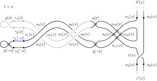
Figure 18: The crossings of $R^{\prime}(x)$ in the variable gadget in case $\ell=x$.

Now we perform a similar inspection as in the proof of Claim 10.1. This time $c=0$, thus we do not allow any internal crossing on arcs $\alpha$ and $\beta$. Most of the cases are straightforward and we refer to Table 2 for the possible $\alpha$ and $\beta$; $\delta^{\prime}(x)$ and $\varepsilon^{\prime}(x)$ play the same role as in the proof of the previous claim. The only exception is that we need to rule out the case $r=q[\ell]$ separately:

Choice of $r$	$t(r)$ in $\alpha$	$t(r)$ in $\beta$	Overlap
$p[\neg\ell]$ if $\ell=x$	$\gamma_{2}[\neg\ell],s_{3}(x),s_{4}(x),q[\neg\ell]$	$\gamma_{1}[\neg\ell],s_{6}(x),s_{8}(x),q[\neg\ell]$	$q[\neg\ell]$
$p[\neg\ell]$ if $\ell=\neg x$	$\gamma_{2}[\neg\ell],s_{7}(x),s_{8}(x),q[\neg\ell]$	$\gamma_{1}[\neg\ell],s_{2}(x),s_{4}(x),q[\neg\ell]$	$q[\neg\ell]$
$q[\ell]$	separate analysis
$q[\neg\ell]$ if $\ell=x$	$s_{4}(x),s_{3}(x),\gamma_{2}[\neg\ell],p[\neg\ell],s_{9}(x)$	$s_{8}(x),s_{6}(x),\gamma_{1}[\neg\ell],p[\neg\ell]$	$p[\neg\ell]$
$q[\neg\ell]$ if $\ell=\neg x$	$s_{8}(x),s_{7}(x),\gamma_{2}[\neg\ell],p[\neg\ell]$	$s_{4}(x),s_{2}(x),\gamma_{1}[\neg\ell],p[\neg\ell],s_{9}(x)$	$p[\neg\ell]$
$s_{9}(x)$	$q[\neg x],s_{10}(x)$	$q[x],s_{11}(x)$	$\emptyset$
$s_{10}(x)$	$s_{9}(x),\delta(x),r(x),\epsilon(x)$	$s_{12}(x)$	$\emptyset$
$s_{11}(x)$	$s_{12}(x)$	$s_{9}(x),r(x),\epsilon(x),\delta(x)$	$\emptyset$
$s_{12}(x)$	$s_{11}(x)$	$s_{10}(x)$	$\emptyset$

Table 2: Possible positions for $t(r)$ depending on $r$ in Claim 10.2.

Let us therefore assume that $r=q[\ell]$. First we want to observe that both $\alpha$ and $\beta$ emanate from $q[\neg\ell]$ to the left. Indeed, if $\alpha$ emanates to the right, then necessarily $\ell=\neg x$ and $t(r)=s_{9}(x)$ but we do not have a suitable $\beta$ for this case. Similarly, if $\beta$ emanates to the right, then $\ell=x$ and $t(r)=s_{9}(x)$ but we do not have a suitable $\alpha$.

Now we know that both $\alpha$ and $\beta$ emanate to the left. This means that both $\alpha$ and $\beta$ are subarcs of the arc with both endpoints $q[\ell]$ left from $q[\ell]$ (if $\ell=x$, this is the grey arc on the Figure 18). In particular, $t(r)$ has to be a selfcrossing of this arc, and there is only one option, namely $t(r)=p[\ell]$. However, here we crucially use Claim 10.1, the twin of $q[\ell]$ cannot be $p[\ell]$ as $p[\ell]$ is removed by a $\rm{I}^{-}$ move. This rules out the case $r=q[\ell]$.

Therefore, it follows from Table 2 that $\{r,t(r)\}=\{p[\neg\ell],q[\neg\ell]\}$. In addition, a further inspection of the variable gadget also reveals that $\alpha$ contains $\gamma_{2}[\neg\ell]$ and $\beta$ contains $\gamma_{1}[\neg\ell]$ as desired. ∎

Now, we have acquired enough tools to finish the proof of the proposition. By Claim 10.1, we have $w(x)\geq 1$ for any variable $x$. By Lemma 7, we deduce

$$\operatorname{def}(\mathbf{D})\geq\sum_{x}w(x)\geq n,$$

where the sum is over all variables. On the other hand, we assume $\operatorname{def}(\mathbf{D})\leq n$. Therefore both inequalities above have to be equalities and in particular $w(x)=1$ for any variable $x$. In particular the assumptions of Claims 10.1 and 10.2 are satisfied for any variable $x$.

Given a variable $x$, we assign $x$ with $\operatorname{TRUE}$ if the conclusion $(i)$ of Claim 10.1 holds (that is, if $x=\ell(x)$). Otherwise, if the conclusion $(ii)$ of Claim 10.1 holds (i.e. $\neg x=\ell(x)$), we set $x$ to $\operatorname{FALSE}$. It remains to prove that we get a satisfying assignment this way.

For contradiction, suppose there is a clause $c=(\ell_{1}\vee\ell_{2}\vee\ell_{3})$ which is not satisfied with this assignment. Let $x_{i}$ be the variable of $\ell_{i}$, that is, $\ell_{i}=x_{i}$ or $\ell_{i}=\neg x_{i}$. The fact that $c$ is not satisfied with the assignment above translates as $\ell(x_{i})=\neg\ell_{i}$ for any $i\in\{1,2,3\}$.

By Claim 10.2, we get that $p[\ell_{i}]$ and $q[\ell_{i}]$ are twins for any $i\in\{1,2,3\}$. Let $R^{\prime\prime}(c)$ be the set of crossings in these Borromeans union the sets $\{p[\ell_{i}],q[\ell_{i}]\}$ for $i\in\{1,2,3\}$. All the crossings in $R^{\prime\prime}(c)$ have weight $0$ and they have to be removed by economical $\rm{II}^{-}$ moves as all defect is realized on points $p[\ell(x)]$ for all variables $x$ (but $p[\ell_{i}]=p[\neg\ell(x_{i})]$ are not among these points).

Let $r$ be the first removed crossing among the crossings in $R^{\prime\prime}(c)$. First, we observe that $r$ cannot be any of $p[\ell_{i}]$ or $q[\ell_{i}]$ for $i\in\{1,2,3\}$. This follows from Claim 10.2 as the arcs $\gamma_{1}[\ell_{i}]$ and $\gamma_{2}[\ell_{i}]$ contain some crossings in $R^{\prime\prime}(c)$.

Next we apply Lemma 9 with $R=R^{\prime\prime}(c)$ and $c=0$. By symmetry of the clause gadget, it is sufficent to consider the cases that $r$ is one of the crossings $u_{1},\dots,u_{8}$ on Figure 19 between the rings for $\ell_{1}$ and $\ell_{2}$.

Figure 19: The clause gadget with crossings $u_{1},\dots,u_{8}$.

Let $\alpha$ and $\beta$ be the arcs between $r$ and $t(r)$ from the definition of $c$-close neighbors. We can immediately rule out $r\in\{u_{4},u_{5},u_{6},u_{7},u_{8}\}$ by an easy inspection as in Claim 10.2 (this is easy because we always hit a crossing from $R^{\prime\prime}(c)$ by possible $\alpha$ and $\beta$). Therefore it remains to consider the case $r\in\{u_{1},u_{2},u_{3}\}$.

Now let us consider the case $r=u_{3}$. The only option for $\alpha$ is to emanate to the left reaching the crossing $u_{1}$ as emanating to the right reaches a crossing from $R^{\prime\prime}(c)$ as an underpass. Consequently, $\beta$ has to emanate to the right since emanating to the left would reach $u_{4}$. However, before $\beta$ reaches $u_{1}$, it has to pass through $p[\ell_{2}]$ or $q[\ell_{2}]$ which rules out this option.

The case $r=u_{2}$ is ruled out analogously.

It remains to consider the case $r=u_{1}$. We have already ruled out the case that the twin $t(r)$ would be $u_{2}$ or $u_{3}$ (it is sufficient to swap $r$ and $t(r)$ in the previous considerations). Thus $\alpha$ has to emanate to the left from $u_{1}$ whereas $\beta$ has to emanate to the right. The first point of $R^{\prime\prime}(c)$ that $\alpha$ reaches is $p[\ell_{1}]$ or $q[\ell_{1}]$ while the first point of $R^{\prime\prime}(c)$ that $\beta$ reaches is $p[\ell_{2}]$ or $q[\ell_{2}]$. Therefore $t(r)$ must be some crossing of $\gamma_{1}[\ell_{1}]$ and $\gamma_{1}[\ell_{2}]$ while $\alpha$ is a subarc of $\gamma_{1}[\ell_{1}]$ and $\beta$ is a subarc of $\gamma_{1}[\ell_{2}]$. On the one hand, such crossing may exist. On the other hand, $\alpha$ reaches such a crossing always as an underpass and $\beta$ as an overpass due to our convention in Step III of the construction of $D(\Phi)$. Therefore, we do not get admissible $\alpha$ and $\beta$. This contradicts the existence of $r$. Therefore, the suggested assignment is satisfying. This finishes the proof.

Part III Hard link invariants

6 Intermediate Invariants

In this section we describe a family of link invariants from the statement of Theorem 2. The material presented here is standard and details can be found in various textbooks; since every piecewise linear knot can be smoothed in a unique way, we assume as we may that the knots discussed are smooth. Throughout Part III we work in the smooth category. We first define:

Definition 11.

Let $L$ be a link in the $3$-sphere. We now give a list of the invariants that we will be using; for a detailed discussion see, for example, [Rol90].

1. A smooth slice surface for $L$ is an orientable surface with no closed components, properly and smoothly embedded in the $4$-ball, whose boundary is $L$. Recall that every link bounds an orientable surface in $S^{3}$ (a Seifert surface); by pushing the interior of that Seifert surface into the $4$-ball we see that every link bounds a smooth slice surface.

2. The $4$-ball Euler characteristic of $L$, denoted $\chi_{4}(L)$, is the largest integer so that $L$ bounds a smooth slice surface of Euler characteristic $\chi_{4}(L)$. Since a smooth slice surface has no closed components, its Euler characteristic is at most the number of components of $L$; in particular, $\chi_{4}(L)$ exists.

3. A link is called smoothly slice if it bounds a slice surface that consists entirely of disks; equivalently, the $\chi_{4}(L)$ equals the number of components of $L$. Note that unlinks are smoothly slice (but not only unlinks).

4. The unlinking number, denoted $u(L)$, is the smallest nonnegative integer so that $L$ admits some diagram $D$ so that after $u(L)$ crossing changes on $D$ a trivial link is obtained.

5. The ribbon number, denoted $u_{r}(L)$, is the smallest nonnegative integer so that $L$ admits some diagram $D$ so that after $u_{r}(L)$ crossing changes on $D$ a ribbon link is obtained (see [Rol90] for the definition of ribbon link).

6. The slicing number, denoted $u_{s}(L)$, is the smallest nonnegative integer so that $L$ admits some diagram $D$ so that after $u_{s}(L)$ crossing changes on $D$ a smoothly slice link is obtained.

7. Links $L_{0},L_{1}\subset S^{3}$ are called concordant if there exists a smooth embedding $f:L_{0}\times[0,1]\rightarrow S^{n}\times[0,1]$, so that $f(L_{0}\times\{0\})=L_{0}\times\{0\}$ and $f(L_{0}\times\{1\})=L_{1}\times\{1\}$. Equivalently, there exists a union of smooth annuli $A$, properly embedded in $S^{3}\times[0,1]$, so that $A\cap(S^{3}\times\{0\})=L_{0}\times\{0\}$ and $A\cap(S^{3}\times\{1\})=L_{1}\times\{1\}$.

8. The concordance unlinking number, denoted $u_{c}(L)$, is the minimum of the unlinking number over the concordance class of $L$.

9. The concordance ribbon number, denoted $u_{cr}(L)$, is the minimum of the ribbon number over the concordance class of $L$.

10. The concordance slicing number, denoted $u_{cs}(L)$, is the minimum of the slicing number over the concordance class of $L$.

11. By transversality, every link $L$ bounds smoothly immersed disks in $B^{4}$ with finitely many double points. The $4$-dimensional clasp number (sometimes called the four ball crossing number) of $L$, denoted $c_{s}(L)$, is the minimal number of double points for such disks.

Finally, we define:

Definition 12 (intermediate invariant).

A real valued link invariant $i$ is called an intermediate invariant if

$$u\geq i\geq c_{s}$$

Many invariants are known to be intermediate (see, for example, [Shi74]). We list a few here:

Lemma 13.

The invariants $u$, $u_{r}$, $u_{s}$, $u_{c}$, $u_{cr}$, $u_{cs}$ and $c_{s}$ are all intermediate.

Proof.

It is well known that the unlink is ribbon and a ribbon link is slice, and therefore

$$u\geq u_{r}\geq u_{s}\text{ and }u_{c}\geq u_{cr}\geq u_{cs}$$

Since any link is in its own concordance class we have

$$u_{s}\geq u_{cs}\text{ and }u\geq u_{c}$$

Combining these we see that

$$u\geq u_{r}\geq u_{s}\geq u_{cs}\text{ and }u\geq u_{c}\geq u_{cr}\geq u_{cs}$$

Therefore it suffices to show that $u_{cs}\geq c_{s}$. To see this, decompose $B^{4}$ (the unit ball in ${\mathbb{R}}^{4}$) as $B^{4}=X_{1}\cup X_{2}\cup X_{3}$ where here:

$$X_{1}=\big{\{}\vec{x}\in{\mathbb{R}}^{4}\ \big{|}\ 0.6<|\vec{x}|\leq 1\big{\}}\ (\cong S^{3}\times(0,1])$$

$$X_{2}=\big{\{}\vec{x}\in{\mathbb{R}}^{4}\ \big{|}\ 0.3<|\vec{x}|<0.7\big{\}}\ (\cong S^{3}\times(0,1))$$

and

$$X_{3}=\big{\{}\vec{x}\in{\mathbb{R}}^{4}\ \big{|}\ |\vec{x}|<0.4\big{\}}\ (\cong\mathrm{int}B^{4})$$

We used open intersections to guarantee smoothness.

Let $L^{\prime}$ be a link in the concordance class of $L$ that minimizes $u_{s}$, that is, $u_{s}(L^{\prime})=u_{cs}(L)$. Since $L$ and $L^{\prime}$ are concordant there exists disjoint annuli $A$, smoothly embedded in $S^{3}\times[0,1]$, so that $A\cap(S^{3}\times\{0\})=L\times\{0\}$ and $A\cap(S^{3}\times\{1\})=L^{\prime}\times\{1\}$. Since $X_{1}\cong S^{3}\times(0,1]$, there exist disjoint annuli $A_{1}$, smoothly embedded in $X_{1}$, so that $A_{1}\cap\partial X_{1}=L$ (note that $\partial X_{1}=S^{3}$) and

$$A_{1}\cap(S^{3}\times(0.6,0.7))=L^{\prime}\times(0.6,0.7)$$

Suppose that $L^{\prime}$ has $\mu$ components and let $k$ denote $u_{s}(L^{\prime})$. Let $L^{\prime\prime}$ be a slice link obtained from $L^{\prime}$ after $k$ crossing changes, and let $S$ denote the disjoint union of $\mu$ circles (so $L^{\prime}$ is an embedding of $S$ into $S^{3}$). Then there is a smooth homotopy $F:S\times(0.3,0.7)\to S^{3}$ realizing $k$ crossing changes, that is:

1. $F(\cdot,t)=L^{\prime}$ for $0.6<t<0.7$.

2. $F(\cdot,t)=L^{\prime\prime}$ for $0.3<t<0.4$.

3. There are $k$ values $0.4<t_{1}<\cdots<t_{k}<.06$ so that $F(\cdot,t_{i})$ has exactly one transverse double point.

4. For any other value $t$ we have that $F(\cdot,t)$ is a smooth embedding of $S$.

Define $\widehat{F}:S\times(0.3,0.7)\to X_{2}$ by

$$\widehat{F}(p,t)=(F(p,t),t)$$

Denote the image of $\widehat{F}$ by $A_{2}$. Then $A_{2}$ are $\mu$ smoothly immersed annuli with exactly $k$ transverse double points. Note that

$$A_{1}\cap(X_{1}\cap X_{2})=A_{2}\cap(X_{1}\cap X_{2})$$

Since $L^{\prime\prime}$ is a smoothly slice link with $\mu$ components it bounds $\mu$ smooth disks disjointly embedded in $B^{4}$. Since $X_{3}\cong\mathrm{int}B^{4}$, this induces a smooth embedding $D\subset X_{3}$, where here $D$ are $\mu$ disks, so that $D\cap(S^{3}\times(0.3,0.4))=L^{\prime\prime}\times(0.3,0.4)$. Note that

$$A_{2}\cap(X_{2}\cap X_{3})=D\cap(X_{2}\cap X_{3})$$

It is now clear that

$$A_{1}\cup A_{2}\cup D$$

is a smooth immersion of $\mu$ disks with exactly $k$ double points, showing that

$$u_{cs}(L)\leq c_{s}(L)$$

∎

Finally we prove:

Lemma 14.

Let $L$ be a link with $\mu$ components. Then

$$\chi_{4}(L)\geq\mu-2c_{s}(L)$$

Sketch of proof.

This was shown by Shibuya [Shi74]; for the convenience of the reader we sketch the proof here. Given $\mu$ disks with $c_{s}(L)$ double points, we endow each disk with an orientation. One can replace a neighborhood of a double point with an annulus in a way that agrees with the chosen orientation. The result is a smooth orientable surface $F$ whose Euler characteristic is $\mu-2c_{s}(L)$. ∎

7 A certain signature calculation.

In this section we calculate the signature of certain links; this will be used in the next section. The signature is an integer valued link invariant, defined for knots by Trotter in [Tro62] and generalized for links by Murasugi in [Mur65].

Since the signature is covered in many standard texts about knots and links we will only summarize how to calculate it:

1. Given a link a $L$, first construct a Seifert surface for $L$, that is, an embedded, orientable surface $F$, with no closed components, whose boundary is $L$. $F$ need not be connected.

2. Next construct embedded oriented curves $\{a_{i}\}$ on $F$ that form a basis for $H_{1}(F;{\mathbb{Z}})$.

3. Arbitrarily fix a co-orientation on each component of $F$ (that is, directions “above” and “below” $F$). We define $a_{i}^{+}$ and $a_{i}^{-}$ to be parallel copies of $a_{i}$ pushed slightly above and below $F$.

4. The Seifert matrix $M$ is the square matrix whose $ij$th entry is $\mathrm{lk}(a_{i}^{+},a_{j}^{-})$, the linking number of $a_{i}^{+}$ and $a_{j}^{-}$. Note that although the linking number is a symmetric function, the matrix $M$ need not be symmetric. Note also that whenever $a_{i}\cap a_{j}=\emptyset$, the $ij$th entry of $M$ is simply $\mathrm{lk}(a_{i},a_{j})$.

5. The signature of $L$, denoted $\sigma(L)$, is the signature of the symmetric bilinear form on $H_{1}(F;{\mathbb{Z}})$ defined by $M+M^{T}$; explicitly, it is the number of positive entries minus the number of negative entries after diagonalizing $M+M^{T}$.

It is quite surprising that $\sigma(L)$ is a link invariant, that is, independent of the choices made. Nevertheless, it is known to be an invariant and a very useful one at that, as we shall see in the next section.

We now define:

Definition 15 (Whitehead Double).

Let $L$ be a link. A Whitehead double of $L$ is a link obtained by taking two parallel copies of each component of $L$ and joining them together with a clasp (see Figure 20). A Whitehead double is called positive if the crossings at the clasp are positive. If the linking number of the two copies of each component is zero the Whitehead double is called untwisted. It is easy to see that the untwisted positive Whitehead double is uniquely determined by $L$.

Figure 20: Some Whitehead doubles

Lemma 16.

The signature of the positive untwisted Whitehead double of the Hopf link is $2$.

Proof.

An untwisted Whitehead double of the Hopf link bounds $F$, two disjointly embedded once punctured tori (see Figure 21). In that figure each torus is seen as a “flat” annulus with a twisted band attached near the top. The tori are co-oriented to the positive side above the “flat” annulus. In that figure we marked $a_{1},a_{2},a_{3},a_{4}$, ordered generators for $H_{1}(F,{\mathbb{Z}})$. This gives the Seifert matrix:

Figure 21: Top: the untwisted Whitehead double of an unknot bounds a flat annulus with a twisted band. Bottom: the positive untwisted Whitehead double of the Hopf link, a Seifert surface and generators of its homology.

$$M=\begin{pmatrix}1&0&0&0\\ 1&0&0&1\\ 0&0&1&0\\ 0&1&1&0\end{pmatrix}$$ (1)

Symmetrizing $M$ we get

$$M+M^{T}=\begin{pmatrix}2&1&0&0\\ 1&0&0&2\\ 0&0&2&1\\ 0&2&1&0\end{pmatrix}$$

A straightforward calculation shows that the signature is $2$. ∎

Before stating the next lemma we describe the type of link we will be dealing with. Let $L$ be a link with an even number of components, say $2n$, so that $L$ can be written as $L=L_{1}\cup\cdots\cup L_{n}$ satisfying the following conditions:

1. $(\forall i)\ L_{i}$ is the positive untwisted Whitehead double of the Hopf link.

2. Each $L_{i}$ bounds $F_{i}$, a co-oriented disjoint union of two once punctured tori, as in Figure 21. Let $a_{1}^{(i)},a_{2}^{(i)},a_{3}^{(i)},a_{4}^{(i)}$ denote the generators for $H_{1}(F_{i};{\mathbb{Z}})$, again as in the figure.

3. $(\forall i\neq i^{\prime})\ \ F_{i}\cap F_{i^{\prime}}=\emptyset$.

4. $(\forall i\neq i^{\prime})(\forall j,j^{\prime})\ \ \mathrm{lk}(a_{j}^{(i)},a_{j^{\prime}}^{(i^{\prime})})=0$.

For a link $L$ as above we have:

Lemma 17.

$\sigma(L)=2n$.

Proof.

With the conventions above we have that $F=F_{1}\cup\cdots\cup F_{n}$ is an oriented Seifert surface for $L$. We will use

$$a_{1}^{(1)},a_{2}^{(1)},a_{3}^{(1)},a_{4}^{(1)},\dots,a_{3}^{(n)},a_{4}^{(n)}$$

as an ordered set of generators for $H_{1}(F;{\mathbb{Z}})$. We obtain a Seifert matrix that along the diagonal has $4\times 4$ identical blocks, each identical to the Seifert matrix of the positive untwisted Whitehead double of the Hopf link (given in (1)). For generators corresponding to $i\neq i^{\prime}$ we have, by assumption, that $\mathrm{lk}(a_{i}^{(j)},a_{i^{\prime}}^{(j^{\prime})})=0$. Thus all the remaining entries are zero. This shows that the signature is the sum of the signatures of the $4\times 4$ blocks, and the lemma follows from Lemma 16. ∎

8 Unlinking, $4$-ball Euler characteristic, and intermediate invariants.

In this section we will show that several link invariants are NP-hard (see the invariants defined in Definition 11). Recall the definition of the positive untwisted Whitehead double (Definition 15 and Figures 20 and 21). One last piece of background we will need is a result of A. Levine [Lev12]. Theorem 1.1 of [Lev12] implies, in particular:

Lemma 18.

The untwisted positive Whitehead double of the Hopf link, and that of the Borromean rings, are not smoothly slice.

We are now ready to describe our construction:

The construction of $L_{\Phi}^{\text{\tiny WH}}$.

Given a 3-SAT instance $\Phi$, recall the link $L_{\Phi}$ from Part I (Figure 1), and let $L_{\Phi}^{\text{\tiny WH}}$ be its positive untwisted Whitehead double. Note that there is a natural bijection between components before and after taking a Whitehead double; let $\kappa_{x_{i}}^{\text{\tiny WH}}$ denote the component corresponding to $\kappa_{x_{i}}$ and let $\kappa_{\neg x_{i}}^{\text{\tiny WH}}$ denote the component corresponding to $\kappa_{\neg x_{i}}$

Remark 19.

If we in addition assume that no clause of $\Phi$ is of the form $(\ell\vee\ell\vee\ell)$ then, by construction, every component of $L_{\Phi}$ is unknotted. Since the Whitehead double of the unknot is unknotted, we may assume that the components of $L_{\Phi}^{\text{\tiny WH}}$ in Theorem 20 are all unknotted.

Recall the definition of intermediate invariants (Definition 12) and the examples given in Lemma 13. The goal of this section is to prove:

Theorem 20.

Given a 3-SAT instance $\Phi$ with $n$ varaibles, let $L_{\Phi}^{\text{\tiny WH}}$ be the link constructed above. Then the following are equivalent, where here $i$ is any intermediate invariant:

1. $\Phi$ is satisfiable.

2. $u(L_{\Phi}^{\text{\tiny WH}})=n$.

3. $i(L_{\Phi}^{\text{\tiny WH}})=n$.

4. $c_{s}(L_{\Phi}^{\text{\tiny WH}})=n$.

5. $\chi_{4}(L_{\Phi}^{\text{\tiny WH}})=0$.

6. $L_{\Phi}^{\text{\tiny WH}}$ admits a smoothly slice sublink with $n$ components.

Theorem 2(b)–(d) directly follows from Theorem 20.

Proof.

The proof of this Theorem is split in the following steps:

1. $\Phi$ is satisfiable implies that $u(L_{\Phi}^{\text{\tiny WH}})\leq n$.

2. $c_{s}(L_{\Phi}^{\text{\tiny WH}})\leq i(L_{\Phi}^{\text{\tiny WH}})\leq u(L_{\Phi}^{\text{\tiny WH}})$.

3. $\chi_{4}(L_{\Phi}^{\text{\tiny WH}})\geq 2n-2c_{s}(L_{\Phi}^{\text{\tiny WH}})$.

4. If $\chi_{4}(L_{\Phi}^{\text{\tiny WH}})\geq 0$ then the following two conditions hold:

   1. $\chi_{4}(L_{\Phi}^{\text{\tiny WH}})=0$

   2. $L_{\Phi}^{\text{\tiny WH}}$ admits a smoothly slice sublink with $n$ components.

5. If $L_{\Phi}^{\text{\tiny WH}}$ admits a smoothly slice sublink with $n$ components, then $\Phi$ is satisfiable.

We first show how (a)—(e) prove Theorem 20. Assume first that $\Phi$ is satisfiable. Then by (a) and (b) we have that $c_{s}(L_{\Phi}^{\text{\tiny WH}})\leq n$, and by (c) we have that $\chi_{4}(L_{\Phi}^{\text{\tiny WH}})\geq 0$. Then (d.I) shows that $\chi_{4}(L_{\Phi}^{\text{\tiny WH}})=0$. Working our way back, we see that $c_{s}(L_{\Phi}^{\text{\tiny WH}})=i(L_{\Phi}^{\text{\tiny WH}})=u(L_{\Phi}^{\text{\tiny WH}})=n$, establishing $(1)\Rightarrow(2)\Rightarrow(3)\Rightarrow(4)\Rightarrow(5)$. In addition, (d.II) shows directly that $(5)\Rightarrow(6)$. Finally, (e) establishes $(6)\Rightarrow(1)$.

We complete the proof of Theorem 20 by establishing (a)—(e):

1. Suppose we have a satisfying assignment for $\Phi$ (for this implication, cf. the proof of Theorem 4). By a single crossing change we resolve the clasp of every component that correspond to a satisfied literal, that is, if $x_{i}=\operatorname{TRUE}$ we change one of the crossings of the clasp of $\kappa_{x_{i}}^{\text{\tiny WH}}$ and if $x_{i}=\operatorname{FALSE}$ we change one of the crossings of the clasp of $\kappa_{\neg x_{i}}^{\text{\tiny WH}}$; as a result, the components corresponding to satisfied literals now form an unlink that is not linked with the remaining components, and we can isotope them away. Since the assignment is satisfying, from each copy of the Borromean rings at least one ring is removed, and the remaining components retract into the first $n$ disks that contained the Hopf links. In each disk we have an untwisted Whitehead double of the unknot which is itself an unknot. Thus we see that the unlink on $2n$ component is obtained, showing that $u(L_{\Phi}^{\text{\tiny WH}})\leq n$.

2. By definition of intermediate invariant we have that $c_{s}\leq i\leq u$.

3. This is Lemma 14.

4. Let $F$ be a slice surface for $L_{\Phi}^{\text{\tiny WH}}$; recall that $F$ has no closed components. We will use the following notation:

   • $\nu$ is the number of components of $F$;

   • $\{F_{i}\}_{i=1}^{\nu}$ are the components of $F$;

   • $g(F_{i})$ and $\#\partial F_{i}$ denote the genus of $F_{i}$ and the number of its boundary components.

   Murasugi [Mur65, Equation 9.4 on Page 416] proved:

   $$\big{|}\sigma(L_{\Phi}^{\text{\tiny WH}})\big{|}\leq 2\Big{(}\sum_{i=1}^{\nu}g(F_{i})\Big{)}+\mu-\nu$$ (2)

   where here $\mu$ denotes the number of components of $L_{\Phi}^{\text{\tiny WH}}$; applying Murasugi’s Theorem with $\mu=2n$ allows us we estimate $\beta_{1}(F)$, the first Betti number of $F$:

   Claim 20.1.

   $\beta_{1}(F)\geq 2n$.

   Proof.

   Since $L_{\Phi}^{\text{\tiny WH}}$ has $2n$ components we have that $\sum_{i=1}^{\nu}\#\partial F_{i}=2n$; this is used in $\star$ below: Since no component of $F$ is closed, $\beta_{1}(F_{i})=2g(F_{i})+\#\partial F_{i}-1$; this is used in $\star\star$ below.

   $$2n =\big{|}\sigma(L_{\Phi}^{\text{\tiny WH}})\big{|}$$ Lemma 17

   $$\leq 2\Big{(}\sum_{i=1}^{\nu}g(F_{i})\Big{)}+2n-\nu \text{Equation}~{}(\ref{equation:murasugi})$$

   $$=\sum_{i=1}^{\nu}\Big{(}2g(F_{i})+\#F_{i}-1\Big{)} \star$$

   $$=\sum_{i=1}^{\nu}\beta_{1}(F_{i}) \star\star$$

   $$=\beta_{1}(F)$$

   This completes the proof of the claim. ∎

   Next we prove:

   Claim 20.2.

   $\nu\geq 2n+\chi(F)$.

   Proof.

   Let $F_{\leq 0}$ be the $\nu-r$ components of $F$ that have nonpositive Euler characteristic; after reordering we may assume that the components of $F_{\leq 0}$ are $F_{1},\dots,F_{\nu-r}$. Since the disk components of $F$ contribute exactly $+r$ to $\chi(F)$ we have

   $$\sum_{i=1}^{\nu-r}\chi(F_{i})=-r+\chi(F)$$

   Solving for $r$ we see:

   $$r =\sum_{i=1}^{\nu-r}\Big{(}-\chi(F_{i})\Big{)}+\chi(F)$$

   $$=\sum_{i=1}^{\nu-r}\Big{(}2g(F_{i})+\#F_{i}-2\Big{)}+\chi(F)$$ (3)

   Disk components contribute zero to $\beta_{1}(F)$, so $\beta_{1}(F)=\sum_{i=1}^{\nu-r}\beta_{1}(F_{i})$. Thus we have (here $\star\star$ is as in Claim 20.1):

   $$\nu =r+(\nu-r)$$

   $$=\sum_{i=1}^{\nu-r}\big{(}2g(F_{i})+\#\partial F_{i}-2\big{)}+\chi(F)+(\nu-r) \text{Equation}~{}(\ref{eq:EulerOfFi})$$

   $$=\sum_{i=1}^{\nu-r}\big{(}2g(F_{i})+\#\partial F_{i}-1\big{)}+\chi(F)$$

   $$=\sum_{i=1}^{\nu-r}\beta_{1}(F_{i})+\chi(F) \star\star$$

   $$=\beta_{1}(F)+\chi(F)$$

   $$\geq 2n+\chi(F)$$ Claim20.1

   This completes the proof of the claim. ∎

   Since $F$ has no closed components we have that $\nu\leq 2n$. Thus by Claim 20.2 we have that $\chi(F)\leq 0$; this establishes Conclusion (d.I).

   Now suppose that $\chi(F)=0$. By Claim 20.2 we have that $\nu=2n$, that is, $F$ has exactly $2n$ components. Thus each component of $F$ has exactly one boundary component. This means that $F_{\leq 0}$ has exactly $2n-r$ components and each has strictly negative Euler characteristic; thus $\chi(F_{\leq 0})\leq-(2n-r)$. The $r$ disk components of $F$ contribute exactly $+r$ to $\chi(F)$ we have that

   $$0=\chi(F)\leq-(2n-r)+r=2r-2n$$

   that is,

   $$n\leq r$$

   By construction, the link formed by the boundaries of the disks $\{F_{\nu-r+1},\dots,F_{\nu}\}$ is an $r$ component smoothly slice sublink of $L_{\Phi}^{\text{\tiny WH}}$, and since $r\geq n$, this establishes Conclusion (d.II).

5. Finally, assume that $L_{\Phi}^{\text{\tiny WH}}$ admits an $n$ component smoothly slice sublink $L_{\text{\tiny SLICE}}$. By Lemma 18 we have that the positive untwisted Whitehead double of the Hopf link is not a sublink of $L_{\text{\tiny SLICE}}$ and therefore for each $i$ exactly one of $\kappa_{x_{i}}^{\text{\tiny WH}}$ and $\kappa_{\neg x_{i}}^{\text{\tiny WH}}$ is in $L_{\text{\tiny SLICE}}$. If $\kappa_{x_{i}}^{\text{\tiny WH}}$ is in $L_{\text{\tiny SLICE}}$ we set $x_{i}=\operatorname{FALSE}$ and if $\kappa_{\neg x_{i}}^{\text{\tiny WH}}$ is in $L_{\text{\tiny SLICE}}$ we set $x_{i}=\operatorname{TRUE}$.

   Using Lemma 18 again we see that $L_{\text{\tiny SLICE}}$ does not admit the positive untwisted Whitehead double of the Borromean rings as a sublink. Therefore, from every set of Borromean rings, at least one component does not belong to $L_{\text{\tiny SLICE}}$; it follows that the assignment above satisfies $\Phi$.

∎

Acknowledgment

We thank Amey Kaloti and Jeremy Van Horn Morris for many helpful conversations.

References

- [AB09] Sanjeev Arora and Boaz Barak. Computational complexity: a modern approach. Cambridge University Press, Cambridge, 2009.
- [AHT06] Ian Agol, Joel Hass, and William Thurston. The computational complexity of knot genus and spanning area. Transactions of the American Mathematical Society, 358:3821–3850, 2006.
- [dMRST18] Arnaud de Mesmay, Yo’av Rieck, Eric Sedgwick, and Martin Tancer. Embeddability in is NP-hard. In Proceedings of the Twenty-Ninth Annual ACM-SIAM Symposium on Discrete Algorithms, pages 1316–1329. Society for Industrial and Applied Mathematics, 2018. Full version on arXiv:1604.00290.
- [Hak61] Wolfgang Haken. Theorie der Normalflächen. Acta Mathematica, 105(3-4):245–375, 1961.
- [HL01] Joel Hass and Jeffrey Lagarias. The number of Reidemeister moves needed for unknotting. Journal of the American Mathematical Society, 14(2):399–428, 2001.
- [HLP99] Joel Hass, Jeffrey C. Lagarias, and Nicholas Pippenger. The computational complexity of knot and link problems. Journal of the ACM (JACM), 46(2):185–211, 1999.
- [HN10] Joel Hass and Tahl Nowik. Unknot diagrams requiring a quadratic number of Reidemeister moves to untangle. Discrete & Computational Geometry, 44(1):91–95, 2010.
- [KL14] Louis H Kauffman and Sofia Lambropoulou. Hard unknots and collapsing tangles. In Introductory Lectures on Knot Theory, 2014.
- [KS] Greg Kuperberg and Eric Samperton. Coloring invariants of knots and links are often intractable. Manuscript.
- [KT18] Dale Koenig and Anastasiia Tsvietkova. NP-hard problems naturally arising in knot theory. arXiv:1602.08427, 2018.
- [Kup14] Greg Kuperberg. Knottedness is in NP, modulo GRH. Adv. Math., 256:493–506, 2014.
- [Lac15] Marc Lackenby. A polynomial upper bound on Reidemeister moves. Ann. Math. (2), 182(2):491–564, 2015.
- [Lac16] Marc Lackenby. The efficient certification of knottedness and Thurston norm. arXiv:1604.00290, 2016.
- [Lac17a] Marc Lackenby. Elementary knot theory. In Lectures on Geometry (Clay Lecture Notes). Oxford University Press, 2017.
- [Lac17b] Marc Lackenby. Some conditionally hard problems on links and 3-manifolds. Discrete & Computational Geometry, 58(3):580–595, 2017.
- [Lev12] Adam Simon Levine. Slicing mixed bing–whitehead doubles. Journal of Topology, 5(3):713–726, 2012.
- [Mur65] Kunio Murasugi. On a certain numerical invariant of link types. Transactions of the American Mathematical Society, 117:387–422, 1965.
- [Pap94] Christos H. Papadimitriou. Computational complexity. Addison-Wesley Publishing Company, Reading, MA, 1994.
- [Rol90] Dale Rolfsen. Knots and links, volume 7 of Mathematics Lecture Series. Publish or Perish, Inc., Houston, TX, 1990. Corrected reprint of the 1976 original.
- [Sam18] Eric Samperton. Computational complexity of enumerative 3-manifold invariants. arXiv preprint arXiv:1805.09275, 2018.
- [Shi74] Tetsuo Shibuya. Some relations among various numerical invariants for links. Osaka J. Math., 11:313–322, 1974.
- [Tro62] Hale F Trotter. Homology of group systems with applications to knot theory. Annals of Mathematics, pages 464–498, 1962.