Continuum Schroedinger operators for sharply terminated graphene-like structures

Abstract.

We study the single electron model of a semi-infinite graphene sheet interfaced with the vacuum and terminated along a zigzag edge. The model is a Schroedinger operator acting on $L^{2}(\mathbb{R}^{2})$: $H^{\lambda}_{\rm edge}=-\Delta+\lambda^{2}V_{\sharp}$, with a potential $V_{\sharp}$ given by a sum of translates an atomic potential well, $V_{0}$, of depth $\lambda^{2}$, centered on a subset of the vertices of a discrete honeycomb structure with a zigzag edge. We give a complete analysis of the low-lying energy spectrum of $H^{\lambda}_{\rm edge}$ in the strong binding regime ($\lambda$ large). In particular, we prove scaled resolvent convergence of $H^{\lambda}_{\rm edge}$ acting on $L^{2}(\mathbb{R}^{2})$, to the (appropriately conjugated) resolvent of a limiting discrete tight-binding Hamiltonian acting in $l^{2}(\mathbb{N}_{0};\mathbb{C}^{2})$. We also prove the existence of edge states: solutions of the eigenvalue problem for $H^{\lambda}_{\rm edge}$ which are localized transverse to the edge and pseudo-periodic (propagating or plane-wave like) parallel to the edge. These edge states arise from a “flat-band” of eigenstates the tight-binding Hamiltonian.

1. Introduction

Tight binding models are discrete models which are central to the modeling of spatially periodic and more general crystalline structures in condensed matter physics. These models apply when the the quantum state of the system is well-approximated by superpositions of translates of highly-localized quantum states (orbitals) within deep atomic potential wells centered at lattice sites [Ashcroft-Mermin:76]. An important example is the tight-binding model of graphene, a planar honeycomb arrangement of carbon atoms with two atoms per unit cell. The two-band tight-binding model yields an explicit approximation for its lowest two dispersion surfaces, which touch conically at Dirac points over the vertices of the Brillouin zone [Wallace:47]. Such Dirac points are central to the remarkable electronic properties of graphene [Kim-etal:05, geim2007rise, RMP-Graphene:09, novoselov2011nobel] and its artificial (electronic, photonic, acoustic, mechanical,…) analogues; see, for example, [artificial-graphene:11, Rechtsman-etal:13a, 2014LuJoannopoulosSoljacic, irvine:15, 2017KhanikaevShvets, Marquardt:17] and the survey [ozawa_etal:18]. The existence of Dirac points for generic honeycomb Schroedinger operators was proved in [FW:12, FLW-MAMS:17]; see also [berkolaiko-comech:18]. That the two-band tight-binding model gives an accurate approximation of the low-lying dispersion surfaces in the regime of strong binding was proved in [FLW-CPAM:17]; see also Section 1.3. Other results on Dirac points for Schroedinger operators on $\mathbb{R}^{2}$ may be found in [Colin-de-Verdiere:91, Grushin:09, ablowitz2009conical, ACZ:12, Lee:16], coupled oscillator models [Makwana-Craster:14] and on quantum graphs in [Kuchment-Post:07, Do-Kuchment:13].

Edge states are modes which are propagating (plane-wave like) parallel to an interface and which are localized transverse to the interface. In condensed matter physics edge states describe the phenomenon of electrical conduction along an interface. Two types of interfaces of great physical interest are a sharp terminations of a bulk structure structure studied in this article (see [Dresselhaus-etal:96, delplace2011zak, mong2011edge, Graf-Porta:13]) and domain wall / line-defects within the bulk (see [2017KhanikaevShvets, Marquardt:17, Rechtsman-etal:18, Sunku:2018qx] and studied, for example, in [FLW-2d_edge:16, FLW-2d_materials:15, LWZ:18, D:19, DW:19] ). The role of edge or surface modes in the spectral theory of Schroedinger operators with potentials which model, for example, the interface between a general periodic medium and a vacuum is studied in e.g. [Davies-Simon:78, Karpeshina:97].

In this paper we study the low-lying energy spectrum (discrete and continuous spectrum) of a sharply terminated honeycomb structure, corresponding to a semi-infinite sheet of graphene joined to the vacuum along a sharp interface. We prove convergence of the operator resolvent to that of a discrete tight-binding model and construct the continuous spectrum of edge states.

Edge states in honeycomb structures such as graphene are of particular interest as foundational building blocks in the field topological insulators (TI). TI’s are materials which are insulating in their bulk and conduction along boundaries, which is robust against large localized perturbations. When graphene is subjected to a magnetic field, its edge currents become unidirectional and acquire such robustness. This phenomenon has an explanation in terms of topological invariants associated with a bulk Floquet-Bloch vector bundle, which takes on non-trivial values when time-reversal symmetry is broken [HK:10, Kane-Mele:05, kane2005quantum].

A key difference between the types of interfaces is that the sharply terminated structure has no spectral gap, resulting in certain edge orientations supporting edge states and others not. In contrast, the domain wall structures perturbations studied in [FLW-2d_edge:16, FLW-2d_materials:15, LWZ:18, D:19, DW:19] have edge states which localize along arbitrary rational edges. For a discussion of the roles played by edge orientation and the type of symmetry breaking in the existence and robustness of edge states for domain wall / line-defects, see [DW:19].

Specifically, for the tight-binding model, edge states exist at sharp terminations along a zigzag edge for a subinterval of parallel quasi-momenta, ${k_{\parallel}}\in[0,2\pi)$ associated with the direction of translation invariance parallel to the edge. They do not exist at the sharp termination along an armchair edge; see, for example, [Dresselhaus-etal:96, delplace2011zak, mong2011edge, Graf-Porta:13] and Section 2. Such results may be interpreted as consequences of the non-vanishing of the Berry-Zak phase, $\mathscr{Z}({k_{\parallel}})$, defined as the integral of the Berry connection over the one-dimensional Brillouin zone associated with the type of edge [delplace2011zak, mong2011edge].

1.1. Mathematical setup

In this paper we initiate a study of these phenomena in the context of the underlying continuum equations of quantum physics, in particular the single-electron model of bulk (infinite) graphene and its terminations. In particular, we study Schroedinger operators on $\mathbb{R}^{2}$ for a sharp termination of a honeycomb structure along a zigzag edge.

We denote the equilateral triangular lattice in $\mathbb{R}^{2}$ by .

(1.1) $$\Lambda\ =\ \mathbb{Z}{\bm{\mathfrak{v}}}_{1}\oplus\mathbb{Z}{\bm{\mathfrak{v}}}_{2}\ ,$$

where ${\bm{\mathfrak{v}}}_{1}$ and ${\bm{\mathfrak{v}}}_{2}$ are given by

(1.8) $${\bm{\mathfrak{v}}}_{1} =\ \left(\begin{array}[]{c}\frac{\sqrt{3}}{2}\\ {}\hfil\\ \frac{1}{2}\end{array}\right),\ \ {\bm{\mathfrak{v}}}_{2}=\ \left(\begin{array}[]{c}0\\ {}\hfil\\ 1\end{array}\right)\ .$$

The dual lattice, $\Lambda^{*}$, is given by

(1.9) $$\Lambda^{*}\ =\ \mathbb{Z}{\bm{\mathfrak{K}}}_{1}\oplus\mathbb{Z}{\bm{\mathfrak{K}}}_{2}\ ,$$

where ${\bm{\mathfrak{K}}}_{1}$ and ${\bm{\mathfrak{K}}}_{2}$ are given by

(1.16) $${\bm{\mathfrak{K}}}_{1}=\ 2\pi\left(\begin{array}[]{c}\frac{2\sqrt{3}}{3}\\ {}\hfil\\ 0\end{array}\right),\ \ \ {\bm{\mathfrak{K}}}_{2}=2\pi\left(\begin{array}[]{c}-\frac{\sqrt{3}}{3}\\ {}\hfil\\ 1\end{array}\right).\$$

Note that

(1.17) $${\bm{\mathfrak{K}}}_{l}\cdot{\bm{\mathfrak{v}}}_{m}=2\pi\delta_{lm}.$$

To generate the honeycomb structure, we first fix base points in $\mathbb{R}^{2}$:

(1.18) $${\bf v}_{A}=(0,0),\qquad{\bf v}_{B}=\left(1/2,1/(2\sqrt{3})\right).$$

The honeycomb structure, $\mathbb{H}$, is the union of the two interpenetrating sublattices

(1.19) $$\Lambda_{A}={\bf v}_{A}+\Lambda,\qquad\Lambda_{B}={\bf v}_{B}+\Lambda\ :$$

(1.20) $$\mathbb{H}\ =\ \Lambda_{A}\ \cup\ \Lambda_{B}\ .$$

Let $V_{0}({\bf x})$ be an atomic potential well which may be considered, for the present discussion, to be radially symmetric, compactly supported with ${\rm supp}\ V_{0}\subset B_{r_{0}}(0)$, the open disc of radius $r_{0}$ about $0$. We discuss more general and physically reasonable conditions on $V_{0}$ below in Section 3.

Our bulk Hamiltonian is the honeycomb Schroedinger operator:

(1.21) $$H_{{}_{\rm bulk}}^{\lambda}\ =\ -\Delta+\lambda^{2}V({\bf x})\ \textrm{acting on $L^{2}(\mathbb{R}^{2})$},$$

where $V({\bf x})$ is a superposition identical atomic potential wells, centered at the vertices of $\mathbb{H}$:

(1.22) $$V({\bf x})=\sum_{{\bf v}\in\mathbb{H}}\ V_{0}({\bf x}-{\bf v})\ ,\ {\bf x}\in\mathbb{R}^{2}\ ,$$

The potential $V({\bf x})$ satisfies the conditions of a honeycomb lattice potential in the sense of Definition 2.1 of [FW:12]. For all but a discrete subset of values of $\lambda$ (including $\lambda=0$), the operator $H_{{}^{\rm bulk}}^{\lambda}$ has Dirac points at energy / quasi-momentum pairs, $(E_{D}^{\lambda},{\bf K}_{\star})$, where ${\bf K}_{\star}$, varies over the vertices of the Brillouin zone [FW:12, FLW-MAMS:17]; see also [berkolaiko-comech:18]. Moreover, for $\lambda$ large (strong binding), the low-lying Floquet-Bloch dispersion surfaces of $H_{{}_{\rm bulk}}^{\lambda}$, when rescaled, are uniformly approximated by the dispersion surfaces of the two-band tight-binding model [FLW-CPAM:17].

Consider now a “half-plane” of vertices $\mathbb{H}_{\sharp}\subset\mathbb{H}$, whose extreme points trace out a zigzag pattern:

(1.23) $$\mathbb{H}_{\sharp}\ \equiv\{{\bf v}_{A}\ +\ \mathbb{N}_{0}{\bm{\mathfrak{v}}}_{1}\oplus\mathbb{Z}{\bm{\mathfrak{v}}}_{2}\}\ \ \cup\ \ \{{\bf v}_{B}\ +\ \mathbb{N}_{0}{\bm{\mathfrak{v}}}_{1}\oplus\mathbb{Z}{\bm{\mathfrak{v}}}_{2}\},\qquad\mathbb{N}_{0}=\{0,1,2,\dots\},$$

The set $\mathbb{H}_{\sharp}$ is invariant with respect to translations by ${\bm{\mathfrak{v}}}_{2}$ and is the subset of sites in $\mathbb{H}$ to the right of an infinite zigzag edge; see Figure 1. The set of zigzag edge (boundary) sites, also translation invariant by ${\bm{\mathfrak{v}}}_{2}$, is given by: $\{{\bf v}_{A}\ +\ \mathbb{Z}{\bm{\mathfrak{v}}}_{2}\}\ \ \cup\ \ \{{\bf v}_{B}\ +\ \mathbb{Z}{\bm{\mathfrak{v}}}_{2}\}$ .

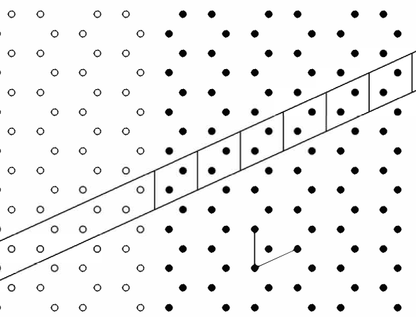
Figure 1. (a) $\mathbb{H}$: Bulk honeycomb structure consists of all vertices (circles, light and dark). (b) $\mathbb{H}_{\sharp}$: Honeycomb structure terminated along a zigzag edge consists of vertices indicated by dark circles; see (1.23). (c) $\Omega_{\Sigma}$: Indicated strip is a choice of fundamental cell for the cylinder $\Sigma=\mathbb{R}^{2}/\mathbb{Z}{\bm{\mathfrak{v}}}_{2}$. $\Omega_{\Sigma}=\Omega_{-1}\cup\Omega_{0}\cup\Omega_{1}\cup\cdots\cup\Omega_{n}\cup\cdots$. Sites: ${\bf v}_{A}^{n},{\bf v}_{B}^{n}$ in finite parallelograms $\Omega_{n}$, $n\geq 0$, are sites in $\mathbb{H}_{\sharp}$. $\Omega_{-1}$ denotes the infinite parallelogram containing no vertices of the terminated structure, $\mathbb{H}_{\sharp}$. 

We define the potential

(1.24) $$V_{\sharp}({\bf x})=\sum_{{\bf v}\in\mathbb{H}_{\sharp}}\ V_{0}({\bf x}-{\bf v})\ ,\qquad\ {\bf x}\in\mathbb{R}^{2}\ .$$

The operator

$$H^{\lambda}_{{}_{\rm edge}}=-\Delta+\lambda^{2}V_{\sharp}({\bf x})$$

models a half-plane of graphene interfaced with the vacuum along a zigzag edge. Note the translation invariance: $V_{\sharp}({\bf x}+{\bm{\mathfrak{v}}}_{2})=V_{\sharp}({\bf x})$ for all ${\bf x}\in\mathbb{R}^{2}$.

Let $(E_{0}^{\lambda},p_{0}^{\lambda}({\bf x}))$, with $p_{0}^{\lambda}>0$ and $L^{2}-$ normalized, denote the ground state eigenpair of the atomic Hamiltonian

$$H^{\lambda}_{\rm atom}=-\Delta+\lambda^{2}V_{0}({\bf x}).$$

Let $\rho_{\lambda}$ denote the hopping coefficient, given by:

(1.25) $$\rho_{\lambda}\ =\ \int_{|{\bf y}|<r_{0}}\ p_{{}_{0}}^{\lambda}({\bf y})\lambda^{2}\ |V_{0}({\bf y})|\ p_{0}^{\lambda}({\bf y}-{\bf e})\ d{\bf y}\ ,$$

where ${\bf e}$ is any vector from one lattice site in $\mathbb{H}$ to a nearest neighbor in $\mathbb{H}$, e.g. ${\bf v}_{B}-{\bf v}_{A}$. The potential $V_{0}({\bf y})$ and ground state $p_{{}_{0}}^{\lambda}({\bf y})$ are localized around ${\bf y}=0$, while $p_{0}^{\lambda}({\bf y}-{\bf e})$, is localized at any nearest neighbor site ${\bf e}\in\mathbb{H}$. Recall that $\text{supp}\ V_{0}$ is contained in the set where $|{\bf x}|<r_{0}$. For $\lambda$ large $\rho_{\lambda}$ is exponentially small (see (3.3)) [FLW-CPAM:17].

The key accomplishments of this paper are the following:

1. Theorem 1.1 (Scaled resolvent convergence): We prove for $\lambda\geq\lambda_{\star}$ sufficiently large (the strong binding regime), that the re-centered and scaled resolvent $\left(\ (H^{\lambda}_{{}_{\rm edge}}-E_{0}^{\lambda})/\rho_{\lambda}-zI\ \right)^{-1}$ has a universal limit (in the uniform operator norm) described by a discrete (tight-binding) Hamiltonian, defined on a truncated honeycomb structure. The band structure of this limiting operator is displayed in Figure 2.
   

2. Theorem 1.2 (Zigzag edge states): We construct a continuum of edge state modes. These are eigenstates of $H^{\lambda}_{{}_{\rm edge}}$, which are propagating (plane-wave like) parallel to and localized transverse to the zigzag edge. Upon appropriate $\lambda-$ dependent rescaling, these edge-states are close to (and converge as $\lambda$ tends to infinity to) the flat band of zero energy edge states of the tight-binding model; see Figure 2.
   

3. Resolvent kernel bounds on arbitrary discrete sets: The methods of this article go considerably beyond those our previous article on the strong binding regime [FLW-CPAM:17], which established convergence to the (universal) two-band tight binding spectrum for the bulk graphene-like structures. Since Theorems 1.1 and 1.2 involve convergence of operators and eigenstates on an infinite cylinder (Figure 1), we required pointwise decay properties of the resolvent kernel $H^{\lambda}_{{}_{\rm edge}}$ for energies near $E_{0}^{\lambda}$. These bounds are stated in Theorem 10.1. In Proposition 10.15 we establish these kernel estimates for potentials which are a sum of atomic potentials centered on an arbitrary discrete set of lattice sites $\Gamma\subset\mathbb{R}^{2}$ (not necessarily translation invariant) whose minimal pairwise distance is $Mr_{0}$, where $r_{0}$ is the radius of the support of $V_{0}$ and $M>2$ is some positive constant. We then specialize to a translation invariant set to obtain Theorem 10.1. We believe the technique we have developed will be quite broadly applicable.

We next introduce the edge state eigenvalue problem. Associated with the translation invariance of $-\Delta+\lambda^{2}V_{\sharp}({\bf x})$ by ${\bm{\mathfrak{v}}}_{2}$ is a parallel quasi-momentum, denoted ${k_{\parallel}}\in[0,2\pi)$. The condition that an edge state, $\Phi$, is propagating parallel to the zigzag edge is:

(1.26) $$\Phi({\bf x}+{\bm{\mathfrak{v}}}_{2})\ =\ e^{i{k_{\parallel}}}\ \Phi({\bf x}),\ \ {\bf x}\in\mathbb{R}^{2}\ \ .$$

We introduce the cylinder

(1.27) $$\Sigma=\mathbb{R}^{2}/\mathbb{Z}{\bm{\mathfrak{v}}}_{2}.$$

The space $L^{2}(\Sigma)$ consists of functions which are square integrable over a fundamental cell of $\Sigma$, e.g. the strip $\Omega_{\Sigma}$ shown in Figure 1, and which satisfy the periodic boundary condition with respect to ${\bm{\mathfrak{v}}}_{2}$: $\phi({\bf x}+{\bm{\mathfrak{v}}}_{2})\ =\ \phi({\bf x})$ for almost all ${\bf x}\in\Omega_{\Sigma}$ and all ${\bf v}\in\Lambda$.

We enforce the condition that (i) $\Phi$ is ${k_{\parallel}}-$ pseudo-periodic parallel to the zigzag edge, (1.26), and (ii) decaying to zero transverse to the zigzag edge as ${\bf x}$ tends to infinity by requiring

$$e^{-i\frac{{k_{\parallel}}}{2\pi}{\bm{\mathfrak{K}}}_{2}\cdot{\bf x}}\Phi({\bf x})\in L^{2}(\Sigma).$$

For such functions we write $\Phi\in L^{2}_{k_{\parallel}}(\Sigma)$ or just $\Phi\in L^{2}_{k_{\parallel}}$. We can now formulate the

${k_{\parallel}}-$Zigzag Edge State Eigenvalue Problem for $H^{\lambda}_{{}_{\rm edge}}=-\Delta+V_{\sharp}({\bf x})$:

(1.28) $$H^{\lambda}_{{}_{\rm edge}}\Psi({\bf x})\ \equiv\ \left(\ -\Delta+\lambda^{2}V_{\sharp}({\bf x})\ \right)\ \Psi({\bf x})\ =\ E\ \Psi({\bf x}),\ \ {\bf x}\in\mathbb{R}^{2},\qquad\Psi\in L^{2}_{k_{\parallel}}(\Sigma).$$

Defining $\Psi({\bf x})=e^{i\frac{{k_{\parallel}}}{2\pi}{\bm{\mathfrak{K}}}_{2}\cdot{\bf x}}\psi({\bf x})$, we may formulate (1.28) equivalently as:

(1.29) $$H^{\lambda}_{{}_{\rm edge}}({k_{\parallel}})\psi\ \equiv\ \left(\ -\left(\nabla+i\frac{{k_{\parallel}}}{2\pi}{\bm{\mathfrak{K}}}_{2}\right)^{2}+\lambda^{2}V_{\sharp}({\bf x})\ \right)\ \psi({\bf x})\ =\ E\ \psi({\bf x}),\ \ {\bf x}\in\mathbb{R}^{2},\qquad\psi\in L^{2}(\Sigma)\ .$$

We refer to non-trivial solutions of the eigenvalue problem (1.28) (equivalently (1.29)) as zigzag edge states.

Before stating our main results Theorems 1.1 and 1.2, we recall a key observation used in [FLW-CPAM:17] to obtain the low-lying dispersion surfaces (energies near the atomic ground state energy, $E_{0}^{\lambda}$) of the bulk honeycomb Schroedinger operator, $H^{\lambda}_{{}_{\rm bulk}}$. That is, for $\lambda$ large, the ${\bf k}-$ pseudo-periodic Floquet-Bloch eigenmodes which are associated with the two lowest spectral bands of $H^{\lambda}_{{}_{\rm bulk}}$, acting in $L^{2}(\mathbb{R}^{2})$, can be uniformly approximated by appropriate linear combinations of the two ${\bf k}-$ pseudo-periodic functions: $P_{{\bf k},I}^{\lambda}({\bf x}),\ I=A,B$. These functions are constructed as ${\bf k}-$ pseudo-periodic weighted sums of translates, $p_{0}^{\lambda}({\bf x}+{\bf v})$, of the atomic ground state, where ${\bf v}$ varies over the sublattices: $\Lambda_{I}={\bf v}_{I}+\Lambda,\ I=A,B$ .

In the present work, to study the low-lying spectral bands associated with eigenvalue problem $H^{\lambda}_{{}_{\rm edge}}({k_{\parallel}})\psi_{k_{\parallel}}^{\lambda}=E^{\lambda}({k_{\parallel}})\psi_{k_{\parallel}}$, $\psi_{k_{\parallel}}^{\lambda}\in L^{2}(\Sigma)$ with $E^{\lambda}({k_{\parallel}})$ near $E_{0}^{\lambda}$ and we find it very natural to approximate eigenstates by superpositions of the infinite family of functions

(1.30) $$p_{{I},{k_{\parallel}}}^{\lambda}[n]({\bf x})\ \in\ L^{2}(\Sigma),\qquad I=A,B,\qquad n\geq 0\ ,$$

which are constructed as ${k_{\parallel}}-$ dependent and periodized (infinite) sums of translates of the ground state $p_{0}^{\lambda}({\bf x})$ over the one-dimensional sublattices: ${\bf v}_{I}+n{\bm{\mathfrak{v}}}_{1}+\mathbb{Z}{\bm{\mathfrak{v}}}_{2}$ of $\Lambda_{I},\ I=A,B$ and $n\geq 0$; see (1.19). The states $p_{{I},{k_{\parallel}}}^{\lambda}[n]({\bf x})$ are introduced in Definition 4.1 in Section 4. For $\lambda$ sufficiently large, any $F\in L^{2}(\Sigma)$ has the expansion

(1.31) $$F=\sum_{I=A,B}\sum_{n\geq 0}\alpha_{n}^{I}\ p_{{I},{k_{\parallel}}}^{\lambda}[n]({\bf x})+F_{\perp},$$

where $\{\alpha_{n}^{I}\}\in l^{2}(\mathbb{N}_{0};\mathbb{C}^{2})$ and $F_{\perp}$ is $L^{2}(\Sigma)-$ orthogonal to the span of the functions $p_{{I},{k_{\parallel}}}^{\lambda}[n]$; see Proposition 4.4. The tight-binding (discrete) edge Hamiltonian, $H^{\rm TB}_{\sharp}({k_{\parallel}})$ acting in $l^{2}(\mathbb{N}_{0};\mathbb{C}^{2})$, arises via translation and rescaling, of the operator whose matrix elements are $\left\langle p_{{J},{k_{\parallel}}}^{\lambda}[m],H_{{}_{\rm edge}}^{\lambda}({k_{\parallel}})p_{{I},{k_{\parallel}}}^{\lambda}[n]\right\rangle_{L^{2}_{k_{\parallel}}}$, for $J,I=A,B$ and $m,n\geq 0$. The tight-binding model is studied in Section 2 and its band spectrum is displayed in Figure 2.

1.2. Main results

The relation of $H_{{}_{\rm edge}}^{\lambda}({k_{\parallel}})$ to the tight-binding Hamiltonian $H^{{}^{\rm TB}}_{\sharp}({k_{\parallel}})$ is given by the following result on scaled resolvent convergence.

Theorem 1.1 (Scaled resolvent convergence).

As in Theorem 1.2, assume that $E_{0}^{\lambda}$, the ground state energy of the atomic Hamiltonian, $H^{\lambda}_{\rm atom}=-\Delta+\lambda^{2}V_{0}$, satisfies the conditions (GS) (3.4) and (EG) (3.6) on the ground state energy and energy-gap, respectively.

Let $\mathscr{C}$ denote a compact subset of $\mathbb{C}\setminus\sigma(H^{{}^{\rm TB}}_{\sharp}({k_{\parallel}}))$, the resolvent set of $H^{{}^{\rm TB}}_{\sharp}({k_{\parallel}})$. There exist constants $\lambda_{\star}$, $C_{\star}$ and $c$, which are independent of $\lambda$ but which depend on $\mathscr{C}$ and conditions (GS) and (EG), such that for all $\lambda>\lambda_{\star}$ the following holds:

Let $J_{k_{\parallel}}:L^{2}(\Sigma)\mapsto l^{2}(N_{0};\mathbb{C}^{2})\oplus\textrm{span}\{p_{I,{k_{\parallel}}}^{\lambda}[n]\}^{\perp}$ be defined, via (1.31), $F\mapsto\left(\{\alpha_{n}^{I}[F]\},F_{\perp}\right)^{\top}$.

Then, uniformly in ${k_{\parallel}}\in[0,2\pi]$, we have

(1.32) $$\Big{\|}\ \Big{(}\ \rho_{\lambda}^{-1}\left(H_{{}_{\rm{edge}}}^{\lambda}({k_{\parallel}})-E_{0}^{\lambda}\right)\ -\ z{\rm Id}\ \Big{)}^{-1}\ -\ J_{k_{\parallel}}^{*}\Big{(}\ H^{{}^{\rm TB}}_{\sharp}({k_{\parallel}})\ -\ z{\rm Id}\ \Big{)}^{-1}\ J_{k_{\parallel}}\ \Big{\|}_{{}_{L^{2}(\Sigma)\to L^{2}(\Sigma)}}\ \leq\ C_{\star}\ e^{-c\lambda}.$$

In preparation for our theorem on edge states, we introduce the functions:

(1.33) $$\zeta({k_{\parallel}})=1+e^{i{k_{\parallel}}},\quad\delta_{\rm gap}({k_{\parallel}})=\Big{|}1-|\zeta({k_{\parallel}})|\Big{|}\geq 0,\quad\delta_{\rm max}({k_{\parallel}})=1+|\zeta({k_{\parallel}})|\ .$$

We note that for ${k_{\parallel}}\in[0,2\pi]$ that $\delta_{\rm gap}({k_{\parallel}})=0$ if and only if ${k_{\parallel}}\in\{2\pi/3,4\pi/3\}$.

Theorem 1.2 (Zigzag Edge States).

Assume that $E_{0}^{\lambda}$, the ground state energy of the atomic Hamiltonian, $H^{\lambda}_{\rm atom}=-\Delta+\lambda^{2}V_{0}$, satisfies the conditions (GS) (3.4) and (EG) (3.6) on the ground state energy and energy-gap, respectively. Let $\mathscr{I}$ denote an arbitrary compact subinterval of quasi-momenta:

(1.34) $$\mathscr{I}\subset\subset(2\pi/3,4\pi/3)\setminus\{\pi\}.$$

Thus, $\min_{{k_{\parallel}}\in\mathscr{I}}\delta_{\rm gap}({k_{\parallel}})>0$.

There exists $\lambda_{\star}=\lambda_{\star}(\mathscr{I})>0$ sufficiently large, such that for all $\lambda>\lambda_{\star}$ the following holds:

1. There is a mapping ${k_{\parallel}}\in\mathscr{I}\ \mapsto\ (E^{\lambda}({k_{\parallel}}),\psi^{\lambda}_{k_{\parallel}})$, from parallel quasimomenta ${k_{\parallel}}$ to simple eigenpairs of the family of the ${k_{\parallel}}-$ edge state eigenvalue problem (1.28):

   (1.35) $$H_{{}_{\rm edge}}^{\lambda}({k_{\parallel}})\psi_{k_{\parallel}}\ =\ E^{\lambda}({k_{\parallel}})\ \psi_{k_{\parallel}}^{\lambda},\quad\psi_{k_{\parallel}}\in L^{2}(\Sigma)$$

   $$E^{\lambda}({k_{\parallel}})\ =\ E_{0}^{\lambda}+\rho_{\lambda}\ \Omega^{\lambda}({k_{\parallel}}),$$

   where $\left|\ \Omega^{\lambda}({k_{\parallel}})\ \right|\ \lesssim\ e^{-c\lambda}$ with $c>0$ independent of $\lambda$. Correspondingly, the eigenvalue problem (1.28) is solved by the states $\Psi^{\lambda}_{k_{\parallel}}({\bf x})=e^{i\frac{{k_{\parallel}}}{2\pi}{\bm{\mathfrak{K}}}_{2}\cdot{\bf x}}\psi_{k_{\parallel}}^{\lambda}({\bf x})$.

2. The edge states $\psi^{\lambda}_{k_{\parallel}}\in L^{2}_{k_{\parallel}}(\Sigma)$ are approximated to within $\mathcal{O}(e^{-c\lambda})$ error in $L^{2}(\Sigma)$ as:

   (1.36) $$\psi^{\lambda}_{k_{\parallel}}({\bf x})\ =\ \sum_{n\geq 0}\ \alpha_{A}^{n}\ p_{A,{k_{\parallel}}}^{\lambda}[n]({\bf x})\ +\ \sum_{n\geq 0}\ \alpha_{B}^{n}\ p_{B,{k_{\parallel}}}^{\lambda}[n]({\bf x})\ +\ \mathcal{O}_{L^{2}(\Sigma)}(e^{-c\lambda}),$$

   where $c>0$ is independent of $\lambda$. Here, $\psi_{k_{\parallel}}^{\rm TB,bd}\ \equiv\ \{\ \left(\alpha^{n}_{A},\alpha^{n}_{B}\right)^{\top}\ \}_{n\geq 0}\ \in\ l^{2}(\mathbb{N}_{0};\mathbb{C}^{2})$, $\|\psi_{k_{\parallel}}^{\rm TB,bd}\|_{{}_{l^{2}(\mathbb{N}_{0};\mathbb{C}^{2})}}\ =\ 1$ is a zero energy normalized eigenstate of the limiting tight-binding edge Hamiltonian; $H^{{}^{\rm TB}}_{\sharp}({k_{\parallel}})\ \psi_{k_{\parallel}}^{\rm TB,bd}=0$. See Theorem 2.2 in Section 2.

Remark 1.3 (Symmetry of edge state curves).

Let ${k_{\parallel}}\in[0,\pi]$. If $\left(E^{\lambda}({k_{\parallel}}),\Psi^{\lambda}_{k_{\parallel}}({\bf x})\right)$ is an eigenpair of the ${k_{\parallel}}-$ edge state eigenvalue problem, then $\left(E^{\lambda}({k_{\parallel}}),\overline{\Psi_{k_{\parallel}}^{\lambda}({\bf x})}\right)$ is an eigenpair of the $2\pi-{k_{\parallel}}$ edge state eigenvalue problem.

Remark 1.4 (Non-flatness of band).

The large $\lambda$ edge states of eigenfrequencies, $E^{\lambda}({k_{\parallel}})$, in Theorem 1.2 arise from the flat band of edge states, $\Omega({k_{\parallel}})=0$ for $2\pi/3<{k_{\parallel}}<4\pi/3$, of the tight-binding Hamiltonian, $H^{{}^{\rm TB}}_{\sharp}({k_{\parallel}})$. Although $E^{\lambda}({k_{\parallel}})$ has only exponentially small variation, we do not expect $E^{\lambda}({k_{\parallel}})$ to be identically constant. Indeed, numerical simulations illustrate the weak variation in ${k_{\parallel}}$ [TWL:19].

Remark 1.5 (Regularity).

We do not address the question of smoothness of ${k_{\parallel}}\in\mathscr{I}\mapsto\left(E^{\lambda}({k_{\parallel}}),\psi^{\lambda}_{k_{\parallel}}\right)\in\mathbb{R}\times L^{2}(\Sigma)$ in the present article. We believe however that the methods of [FLW-CPAM:17] may be adapted to show that this mapping extends as an analytic mapping in a complex neighborhood of $\mathscr{I}$ from which derivative bounds, e.g. on $E^{\lambda}({k_{\parallel}})$ (${k_{\parallel}}\in\mathscr{I}$) can be derived via Cauchy estimates.

Remark 1.6.

In Theorem 2.2 we find: $\psi_{k_{\parallel}}^{\rm TB,bd}=\sqrt{1-|\zeta({k_{\parallel}})|^{2}}\Big{(}\ [-\zeta({k_{\parallel}})]^{n},0\ \Big{)}^{\top}$. Therefore, at leading order, $\Psi^{\lambda}_{k_{\parallel}}({\bf x})$ is concentrated about the $A-$ sublattice, $\Lambda_{A}$:

(1.37) $$\Psi^{\lambda}_{k_{\parallel}}({\bf x})\ =\ \sqrt{1-|\zeta({k_{\parallel}})|^{2}}\ \sum_{n\geq 0}\ [-\zeta({k_{\parallel}})]^{n}\ P_{A,{k_{\parallel}}}^{\lambda}[n]({\bf x})\ +\ \mathcal{O}_{L^{2}_{k_{\parallel}}}(e^{-c\lambda}).$$

Remark 1.7.

As noted in our discussion of the tight-binding model in Section 2 (Remark 2.3) the constraint of Theorem 1.2 on parallel quasimomenta: ${k_{\parallel}}\in(2\pi/3,4\pi/3)$ ($|\zeta({k_{\parallel}})|<1$) corresponds to the non-vanishing of the Zak phase. This is discussed further in Remark 2.3.

Remark 1.8.

In work in progress we show, for a sharp termination of the bulk honeycomb structure along an armchair edge, that there are no edge states in an energy range about $E_{0}^{\lambda}$. In this case, the relevant Zak phase vanishes for all ${k_{\parallel}}\in[0,2\pi]$.

1.3. Relation to previous work

Tight-binding limits arising from general distributions of potential wells has been discussed in the book of [DiMassi-Sjoestrand:99] as well as [Outassourt:87, Carlsson:90]. There is extensive related earlier work on the semiclassical limits and methods e.g. [Simon:83, Simon:84a, Simon:84b, Helffer-Sjoestrand:84, Helffer:88, Chantelau:90, Mohamed:91, Daumer:94, Daumer:96]. The above works are based on detailed semiclassical (WKB) approximations for potential wells which are assumed to have non-degenerate local minima. In contrast, in the present article our essential assumptions are only on the ground state energy (GS) and spectral gap (EG) of the atomic Hamiltonian, $H^{\lambda}_{atom}$ for large $\lambda$. The relation of the continuum periodic Schroedinger operator with a magnetic field to tight-binding models, such as the Harper model, is studied for example in [HS:88].

For convenience we have restricted attention here to $C^{\infty}$ potentials. However, we believe it will be easy to make small changes in our proofs, to apply our results to nonsmooth potentials of interest. In particular, the atomic potential may be taken to have a Coulomb singularity at the origin, or to have the form $V_{0}(x)=-1$ for ${\bf x}$ in a ball $B$, $V_{0}(x)=0$ otherwise. Here the radius of $B$ is taken small enough to satisfy the hypothesis $(PW_{2})$ of Section 3.1 below. Examples of artificial graphene, in which experiments are performed, are periodic honeycomb arrays of identical microfeatures, say small discs, with one dielectric constant inside the discs and a second dielectric constant outside the discs. Hence, compactly supported atomic potentials are a natural model; see, for example, [artificial-graphene:11, Rechtsman-etal:13a, 2014LuJoannopoulosSoljacic, irvine:15, 2017KhanikaevShvets, Marquardt:17, ozawa_etal:18].

For smooth atomic potentials $V_{0}$ with nondegenerate minima, the general semiclassical works in [DiMassi-Sjoestrand:99, Outassourt:87, Carlsson:90] lead to an “interaction matrix”, which defines an operator. In the case of periodic potentials, this can be used to compute relevant dispersion surfaces modulo exponentially small errors. These works do not assert that Dirac points form; indeed, much of the work is in the setting of a square lattice, which does not give rise to Dirac points. However, we believe that these methods are powerful enough to deal with Dirac points of honeycomb lattice potentials, when they are combined with the consequences of special symmetry properties of the honeycomb. The essential requirement for the semiclassical analysis approach is that the atomic potential is smooth and has a nondegenerate minimum. Another aspect of the general work of this semiclassical work is that atomic potentials are not assumed to be of compact support and the interaction matrix (hopping coefficients) are obtained in terms of the Agmon metric. Finally, the consideration of edge states and the spectrum for honeycombs with line defects is not within the scope of [DiMassi-Sjoestrand:99, Outassourt:87, Carlsson:90].

Remark 1.9.

A different class of line-defects of great interest in the study of topologically protected edge states is the class of domain walls. In our previous work, motivated by [HR:07, RH:08, Soljacic-etal:08], domain walls are realized by starting with two periodic structures at “ $+\infty$ ” and “ $-\infty$ ”, with a common spectral gap and phase-shifted from one another, and connecting them across a line-defect at which there is no phase-distortion. See the analytical work in 1D [FLW-PNAS:14, FLW-MAMS:17, DFW:18] and 2D [FLW-2d_edge:16, FLW-2d_materials:15, LWZ:18] as well as theoretical and experimental work on photonic realizations [Thorp-etal:15, CLEO-Thorp_etal:16, CLEO-Poo_etal:16].

Remark 1.10.

Quantum graphs [BK:13] are another class of discrete models in condensed matter, electromagnetic and other systems; see also, for example, [Shipman:17, Becker-Zworski:18, BHJ:18]. An extensive discussion of edge states for nanotube structures in the setting of quantum graphs is given in [Kuchment-Post:07, Do-Kuchment:13]. It would be of interest to investigate a relation between the edge modes of these models and continuum models.

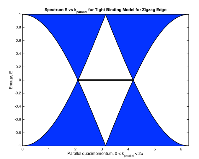
Figure 2. Spectrum of tight-binding Hamiltonian $H^{{}^{\rm TB}}_{\sharp}({k_{\parallel}})$, for $0\leq{k_{\parallel}}\leq 2\pi$, described in Theorem 2.2. This spectrum contains a flat band of zero energy states; $H^{\lambda}_{\sharp}({k_{\parallel}})$ has an isolated simple $0-$ energy eigenstate for $2\pi/3\leq{k_{\parallel}}\leq 4\pi/3$. Shaded regions consist of continuous spectrum. For sufficiently large $\lambda$, the low-lying part of the spectrum of $-\Delta+\lambda^{2}V_{\sharp}-E_{0}^{\lambda}$, after rescaling by $\rho_{\lambda}$, is approximated by spectrum of the 2-band model $H^{{}^{\rm TB}}_{\sharp}$; see Theorem 1.2.

1.4. Outline of the paper

We present a brief outline.

1. Section 2 discusses tight binding models; first, the tight binding model for bulk, and then the tight binding model for a honeycomb structure terminated along a zigzag edge.
   

2. Section 3 first introduces the atomic Hamiltonian $H^{\lambda}_{\rm atom}=-\Delta+V_{0}$, where $V_{0}$ is a potential well whose support in a sufficiently small disc about the origin, and such that $V_{0}$ satisfies some basic general assumptions $(PW_{1})-(PW_{4})$. The bulk honeycomb structure is defined by $H^{\lambda}_{\rm bulk}=-\Delta+\lambda^{2}V$, where $V$ is the periodic potential by summing $V_{0}$ over translates of the atomic potential, $V_{0}$, over the honeycomb structure. Thus $V$ consists of a potential well $V_{0}$ centered at each site of the honeycomb. Finally the edge Hamiltonian, $H_{\rm edge}=-\Delta+\lambda^{2}V_{\sharp}$, which acts on $L^{2}(\mathbb{R}^{2})$, has potential $V_{\sharp}$ which is identically equal to $V$ on a half-space with a zigzag edge and zero on the other side of this zigzag edge. (We shall also work with the translated edge Hamiltonian $H^{\lambda}_{\sharp}=H_{\rm edge}-E_{0}^{\lambda}$.) The edge state eigenvalue problem for parallel quasi-momentum ${k_{\parallel}}$ is then stated on $L^{2}(\Sigma)$, where $\Sigma$ is the infinite cylinder (1.27).
   

3. Section 4 introduces a natural basis for approximating the 2 lowest lying bands of $H^{\lambda}_{\sharp}$ for $\lambda$ sufficiently large. This basis consists of functions, $\{p_{{I},{k_{\parallel}}}^{\lambda}[n]({\bf x}):{I}=A,B,n\geq 0\}$ on $\Sigma$, which are pseudo-periodic (with respect to the direction parallel to the edge) infinite sums of atomic orbitals.
   

4. Section 5 establishes energy estimates on $H^{\lambda}_{\sharp}$ which imply invertibility of $H^{\lambda}_{\sharp}$ on $\mathscr{X}_{AB}({k_{\parallel}})$, the orthogonal complement of the orbital subspace: ${\rm span}\{p^{\lambda}_{I,{k_{\parallel}}}[n]:n\geq 0,I=A,B\}$. This implies that the resolvent of $H^{\lambda}_{\sharp}$ is well-defined and bounded on $\mathscr{X}_{AB}({k_{\parallel}})$ .
   

5. Section 6 implements a Lyapunov-Schmidt / Schur complement reduction strategy: The spectral problem on $L^{2}(\Sigma)={\rm span}\{p^{\lambda}_{I,{k_{\parallel}}}[n]:n\geq 0,I=A,B\}\oplus\mathscr{X}_{AB}({k_{\parallel}})$ is reduced, using the resolvent bounds on $\mathscr{X}_{AB}({k_{\parallel}})$, to an equivalent problem on the space ${\rm span}\{p^{\lambda}_{I,{k_{\parallel}}}[n]:n\geq 0,I=A,B\}$. This problem depends nonlinearly on the eigenvalue parameter $E=E_{0}^{\lambda}+\rho_{\lambda}\Omega$ and is of the form of an infinite algebraic system:

   $$\sum_{I=A,B}\sum_{n\geq 0}\mathcal{M}^{\lambda,{k_{\parallel}}}_{JI}[m,n](\Omega,{k_{\parallel}})\ \alpha_{n}^{I}\ =\ 0;\ \ J=A,B,\ \ m\geq 0$$

   for $(\Omega,\alpha)$, where $\alpha=\{\alpha_{n}^{I}\}_{n\geq 0,I=A,B}\in l^{2}(\mathbb{N}_{0};\mathbb{C}^{2})$ are coordinates relative to the basis $\{p^{\lambda}_{I,{k_{\parallel}}}[n]:n\geq 0,I=A,B\}$.
   

6. Section 7 summarizes the required properties of $\mathcal{M}^{\lambda}(\Omega,{k_{\parallel}})$ acting in $l^{2}(\mathbb{N}_{0};\mathbb{C}^{2})$. We write $\mathcal{M}^{\lambda,{k_{\parallel}}}(\Omega,{k_{\parallel}})=\mathcal{M}_{\rm lin}^{\lambda}(\Omega,{k_{\parallel}})-\mathcal{M}_{\rm nlin}^{\lambda}(\Omega,{k_{\parallel}})$, separating matrix elements contibutions which are linear in $H^{\lambda}_{\sharp}({k_{\parallel}})$ and those which are nonlinear in $H^{\lambda}_{\sharp}({k_{\parallel}})$. We have $\mathcal{M}_{\rm lin}^{\lambda}(\Omega,{k_{\parallel}})=\rho_{\lambda}H^{{}^{\rm TB}}_{\sharp}({k_{\parallel}})\ +\ \mathcal{O}_{l^{2}\to l^{2}}(\rho_{\lambda}e^{-c\lambda})$ (Proposition 7.1) and $\mathcal{M}_{\rm nlin}^{\lambda}(\Omega,{k_{\parallel}})=\mathcal{O}_{l^{2}\to l^{2}}(\rho_{\lambda}e^{-c\lambda})$ (Proposition 7.2). These propositions are proved in later sections.
   

7. Section 8 proves Theorem 1.2, the existence of edge states, bifurcating from the flat band of eigenstates of $H^{{}^{\rm TB}}_{\sharp}$, via our formulation of the eigenvalue in $l^{2}(\mathbb{N}_{0};\mathbb{C}^{2})$.
   

8. Section 9 proves Theorem 1.1, the convergence of a translation and scaling of the resolvent of $H^{\lambda}_{\sharp}({k_{\parallel}})$ to that of $H^{{}^{\rm TB}}_{\sharp}({k_{\parallel}})$.
   

9. Section 10 is the most technically involved and introduces techniques not present in our earlier work. Theorem 10.1 is a pointwise estimate on the resolvent kernel of $H^{\lambda}_{\sharp}-z=H_{\rm bulk}^{\lambda}-(E_{0}^{\lambda}+z)$, $z$ small, when restricted to the orthogonal complement of ${\rm span}\{p^{\lambda}_{I,{k_{\parallel}}}[n]:n\geq 0,I=A,B\}$. These bounds are stated in Theorem 10.1. We first, in Proposition 10.15, establish these kernel estimates for potentials which are a sum of atomic potentials centered on an arbitrary discrete set of lattice sites $\Gamma\subset\mathbb{R}^{2}$ (not necessarily translation invariant), whose minimal pairwise distance is $Mr_{0}$, where $r_{0}$ is the radius of the support of $V_{0}$ and $M>2$ is some positive constant. We then specialize to a translation invariant set to obtain Theorem 10.1.
   

10. Section 11 expands the linear matrix elements, $\mathcal{M}_{\rm lin}^{\lambda}(\Omega,{k_{\parallel}})$, in terms of $H^{{}^{\rm TB}}_{\sharp}({k_{\parallel}})$ and estimates the corrections, proving Proposition 7.1.
    

11. Section 12 estimates the nonlinear matrix elements, $\mathcal{M}_{\rm nlin}^{\lambda}(\Omega,{k_{\parallel}})$, proving Proposition 7.2.
    

12. Finally, there are two appendices. Appendix A introduces a technical tool used to construct the resolvent of $H^{\lambda}_{\sharp}$ on $\mathscr{X}_{AB}^{\lambda}({k_{\parallel}})$. Appendix B contains general results on overlap integrals enabling expansion of $\mathcal{M}_{\rm lin}^{\lambda}(\Omega,{k_{\parallel}})$, for $\lambda$ large, estimate corrections.

1.5. Notation

1. $\mathbb{N}=\{1,2,3,\dots\}$,  $\mathbb{N}_{0}=\{0,1,2,3,\dots\}$ .

2. When we write the expression $g_{\varepsilon}=\mathcal{O}_{X}(\gamma_{\varepsilon})$ as $\varepsilon\to\varepsilon_{0}\in\mathbb{R}\cup\{\infty\}$, we mean that there exists $C>0$, independent of $\varepsilon$, such that $\|g_{\varepsilon}\|_{X}\leq C\gamma_{\varepsilon}$ as $\varepsilon\to\varepsilon_{0}$.

3. We shall be concerned with the asymptotic behavior of many expressions, $a(\lambda),b(\lambda),\dots$, in the regime where the parameter $\lambda$ sufficiently large. The relation $a(\lambda)\lesssim b(\lambda)$ means that there is a constant $C$, which can be taken to be independent of $\lambda$, such that for all $\lambda$ sufficiently large: $a(\lambda)\leq Cb(\lambda)$.

4. $\Lambda=\mathbb{Z}{\bm{\mathfrak{v}}}_{1}\oplus\mathbb{Z}{\bm{\mathfrak{v}}}_{2},$ the equilateral triangular lattice, is generated by the basis vectors ${\bm{\mathfrak{v}}}_{1}$ and ${\bm{\mathfrak{v}}}_{2}$, displayed in (1.8).

5. ${\bf m}\vec{\bm{\mathfrak{v}}}=m_{1}{\bm{\mathfrak{v}}}_{1}+m_{2}{\bm{\mathfrak{v}}}_{2}$, where ${\bf m}=(m_{1},m_{2})\in\mathbb{Z}^{2}$.

6. $\Lambda^{*}=\ \mathbb{Z}{\bm{\mathfrak{K}}}_{1}\oplus\mathbb{Z}{\bm{\mathfrak{K}}}_{2}$, the dual lattice, spanned by the dual basis vectors ${\bm{\mathfrak{K}}}_{1}$ and ${\bm{\mathfrak{K}}}_{2}$, displayed in (1.16). Note that ${\bm{\mathfrak{K}}}_{\ell}\cdot{\bm{\mathfrak{v}}}_{{\ell^{\prime}}}=2\pi\delta_{\ell{\ell^{\prime}}}$.

7. We remark that alternative bases for $\Lambda$ and $\Lambda^{*}$ (used for example in [FW:12, FLW-CPAM:17]) are:

   $${\bf v}_{1} ={\bm{\mathfrak{v}}}_{1},\quad{\bf v}_{2}={\bm{\mathfrak{v}}}_{1}-{\bm{\mathfrak{v}}}_{2}$$

   $${\bf k}_{1} ={\bm{\mathfrak{K}}}_{1}+{\bm{\mathfrak{K}}}_{2},\quad{\bf k}_{2}=-{\bm{\mathfrak{K}}}_{2}.$$

   We have $\Lambda=\mathbb{Z}{\bf v}_{1}\oplus\mathbb{Z}{\bf v}_{2}$, $\Lambda^{*}=\ \mathbb{Z}{\bf k}_{1}\oplus\mathbb{Z}{\bf k}_{2}$ and ${\bf k}_{\ell}\cdot{\bf v}_{{\ell^{\prime}}}=2\pi\delta_{\ell{\ell^{\prime}}}$.

8. $\mathbb{H}$, Honeycomb structure; see (1.20).

9. $\mathbb{H}_{\sharp}$, Zigzag-truncated honeycomb structure; see (1.23).

10. $\Sigma=\mathbb{R}^{2}/\mathbb{Z}{\bm{\mathfrak{v}}}_{2}$, the cylinder with $\Omega_{\Sigma}$, a choice of fundamental cell for $\Sigma$; see Figure 1.

11. $L^{2}_{k_{\parallel}}=L^{2}_{k_{\parallel}}(\Sigma)$, functions $f$ such that $f({\bf x}+{\bm{\mathfrak{v}}}_{2})=e^{i{k_{\parallel}}}f({\bf x})$ for almost all ${\bf x}$, and

    $$\|f\|_{{}_{L^{2}_{k_{\parallel}}}}^{2}\ =\ \int_{{}_{\Omega_{\Sigma}}}|f|^{2}<\infty.$$

12. $\mathscr{H}^{(\omega)}\equiv L^{2}(\mathbb{R}^{2};e^{\gamma|{\bf x}-\omega|}\ d{\bf x})$, exponentially weighted $L^{2}$ space.

13. $\mathcal{B}(X)$ denotes the space of bounded linear operators on $X$.

14. $G_{\lambda}^{\rm free}({\bf x},{\bf y})$ denotes the free Green’s function defined in (10.3).

15. $G_{\lambda}^{\rm atom}({\bf x},{\bf y})$ denotes the atomic Green’s function defined in (10.7).

16. Hamiltonians:
    $H^{\lambda}_{\rm atom}=-\Delta+\lambda^{2}V_{0}({\bf x})$, the atomic Hamiltonian with ground state energy $E_{0}^{\lambda}$
    $H^{\lambda}_{{}_{\rm bulk}}=-\Delta+\lambda^{2}V({\bf x})$ and $H^{\lambda}_{{}_{\rm edge}}=-\Delta+\lambda^{2}V_{\sharp}({\bf x})$, denote bulk and edge Hamiltonians acting in $L^{2}(\mathbb{R}^{2})$
    $H^{\lambda}_{\sharp}=H^{\lambda}_{{}_{\rm edge}}\ -\ E_{0}^{\lambda}$, the centered edge Hamiltonian, acting in $L^{2}_{k_{\parallel}}$
    $\widetilde{H}_{\sharp}^{\lambda}\ =\ (\rho_{\lambda})^{-1}\ H^{\lambda}_{\sharp}$, the scaled and centered edge Hamiltonian acting in $L^{2}_{k_{\parallel}}$
     $H^{{}^{\rm TB}}_{\sharp}({k_{\parallel}})$, the tight-binding edge Hamiltonian, acting in $l^{2}(\mathbb{N}_{0};\mathbb{C}^{2})$; see Definition 2.6.

Acknowledgements: The authors wish to thank Gian Michele Graf and Alexis Drouot for very stimulating discussions. We would also like to thank Bernard Helffer for correspondence concerning previous general results on tight-binding limits. Part of this research was done while MIW was Bergman Visiting Professor at Stanford University. CLF and MIW wish to thank the Department of Mathematics at Stanford University for its hospitality. This research was supported in part by National Science Foundation grants DMS-1265524 (CLF) and DMS-1412560, DMS-1620418 and Simons Foundation Math + X Investigator Award #376319 (MIW).

2. Tight-binding

Consider a tiling of the entire plane, $\mathbb{R}^{2}$, by parallelograms of the sort shown in Figure 1 Each parallelogram has exactly two points of $\mathbb{H}$. This is a particular dimerization of $\mathbb{H}$. We assign the label $(n_{1},n_{2})$ to the parallelogram which contains ${\bf v}_{A}^{(n_{1},n_{2})}={\bf v}_{A}+n_{1}{\bm{\mathfrak{v}}}_{1}+n_{2}{\bm{\mathfrak{v}}}_{2}$ and ${\bf v}_{B}^{(n_{1},n_{2})}={\bf v}_{B}+n_{1}{\bm{\mathfrak{v}}}_{1}+n_{2}{\bm{\mathfrak{v}}}_{2}$. To the sites ${\bf v}_{A}^{(n_{1},n_{2})}$ and ${\bf v}_{B}^{(n_{1},n_{2})}$ we assign complex amplitudes $\psi^{A}_{{}_{n_{1},n_{2}}}$ and $\psi^{B}_{{}_{n_{1},n_{2}}}$ and form the tight binding wave function:

$$\psi_{{}_{n_{1},n_{2}}}=\begin{pmatrix}\psi^{A}_{{}_{n_{1},n_{2}}}\\ \psi^{B}_{{}_{n_{1},n_{2}}}\end{pmatrix}$$

2.1. $H^{{}^{\rm TB}}_{{}_{\rm bulk}}$, the tight-binding bulk Hamiltonian

The bulk tight binding Hamiltonian can be represented with respect to the above dimerization. Starting with any dimerization would give a unitarily equivalent operator on $l^{2}(\mathbb{Z}^{2};\mathbb{C}^{2})$. The nearest neighbor tight binding bulk Hamiltonian, relative to the dimerization of $\mathbb{H}$ in Figure 1 is:

(2.1) $$\left[\ H^{{}^{\rm TB}}_{{}_{\rm bulk}}\psi\ \right]_{{}_{{n_{1}},{n_{2}}}}\ =\ \begin{pmatrix}\left(\ H^{{}^{\rm TB}}_{{}_{\rm bulk}}\psi\ \right)^{A}_{{}_{{n_{1}},{n_{2}}}}\\ \left(\ H^{{}^{\rm TB}}_{{}_{\rm bulk}}\psi\ \right)^{B}_{{}_{{n_{1}},{n_{2}}}}\end{pmatrix}=\begin{pmatrix}\psi_{{}_{n_{1}-1,n_{2}}}^{B}\ +\ \psi_{{}_{n_{1},n_{2}-1}}^{B}\ +\ \psi_{{}_{n_{1},n_{2}}}^{B}\\ \psi_{{}_{n_{1}+1,n_{2}}}^{A}\ +\ \psi_{{}_{n_{1},n_{2}+1}}^{A}\ +\ \psi_{{}_{n_{1},n_{2}}}^{A}\end{pmatrix}$$

where $n_{1},n_{2}\in\mathbb{Z}$. The operator $H_{{}_{\rm bulk}}^{\rm TB}$ is a bounded self-adjoint linear operator on $l^{2}(\mathbb{Z}^{2};\mathbb{C}^{2})$ and was introduced in [Wallace:47]. The spectrum of $H^{{}^{\rm TB}}_{{}_{\rm bulk}}$ consists of two spectral bands which touch conically at Dirac points over the vertices of $\mathcal{B}$. The approximation and convergence as $\lambda$ increases of the low-lying dispersion surfaces and the resolvent $H_{{}_{\rm bulk}}^{\lambda}$ acting on $L^{2}(\mathbb{R}^{2})$ to those of $H_{{}_{\rm bulk}}^{\rm TB}$ acting on $l^{2}(\mathbb{Z}^{2};\mathbb{C}^{2})$ was studied in [FLW-CPAM:17] .

2.2. Tight-binding Hamiltonian for the zigzag edge

Our goal in this section is to introduce a tight-binding edge Hamiltonian which will act on functions $\psi\in l^{2}\left((\mathbb{N}_{0}\times\mathbb{Z});\mathbb{C}^{2}\right)$ defined on the vertices of $\mathbb{H}_{\sharp}$. We shall do this by first expressing $H_{\rm bulk}^{{}^{\rm TB}}$, as a direct integral over ${k_{\parallel}}$ of fiber operators $H_{\rm bulk}^{{}^{\rm TB}}({k_{\parallel}})$ acting on states which are “${k_{\parallel}}$- pseudo-periodic” with respect to one lattice direction and square-summable with respect to the other lattice direction. The edge Hamiltonian $H^{{}^{\rm TB}}_{\sharp}$ is then obtained from $H_{\rm bulk}^{{}^{\rm TB}}({k_{\parallel}})$ by appropriate restriction to functions defined on $\mathbb{H}_{\sharp}$.

Since the truncated structure $\mathbb{H}_{\sharp}$ and its subset edge vertices are invariant with respect to translation by ${\bm{\mathfrak{v}}}_{2}$, we introduce ${k_{\parallel}}\in S^{1}=\mathbb{R}/2\pi\mathbb{Z}$, the parallel quasi-momentum associated with this translation invariance. For each ${k_{\parallel}}\in[0,2\pi]$, we refer to a state as being ${k_{\parallel}}-$ pseudo-periodic if:

(2.2) $$\psi_{n_{1},n_{2}+1}=e^{i{k_{\parallel}}}\psi_{n_{1},n_{2}},\ \ n_{1}\geq 0,\ \ n_{2}\in\mathbb{Z}.$$

Functions $\psi=\{\psi_{{}_{n_{1},n_{2}}}\}\in l^{2}(\mathbb{Z};\mathbb{C}^{2})$ may be expressed via the discrete Fourier transform as

(2.3) $$\psi_{{}_{n_{1},n_{2}}}\ =\ (2\pi)^{-1}\int_{0}^{2\pi}\ e^{i{n_{2}}{k_{\parallel}}}\psi_{{}_{{n_{1}}}}({k_{\parallel}})\ d{k_{\parallel}},$$

as a superposition over states $\{e^{i{n_{2}}{k_{\parallel}}}\psi_{{}_{{n_{1}}}}({k_{\parallel}})\}$ which are square-summable over $\mathbb{Z}$ with respect to $n_{1}$ and which satisfy (2.2).

Therefore, the tight binding bulk Hamiltonian $H^{{}^{\rm TB}}_{\rm bulk}$ may be reduced to the ${k_{\parallel}}-$ dependent fiber (Bloch) Hamiltonians, $H^{{}^{\rm TB}}_{{}_{\rm bulk}}({k_{\parallel}}):l^{2}(\mathbb{Z};\mathbb{C}^{2})\to l^{2}(\mathbb{Z};\mathbb{C}^{2})$, defined by

$$\left[H^{{}^{\rm TB}}_{{}_{\rm bulk}}({k_{\parallel}})\psi\right]_{{}_{{n_{1}}}}\ \equiv\begin{pmatrix}\psi_{{}_{n_{1}-1}}^{B}\ +\ \left(1+e^{-i{k_{\parallel}}}\right)\ \psi_{{}_{n_{1}}}^{B}\\ \psi_{{}_{n_{1}+1}}^{A}\ +\ \left(1+e^{+i{k_{\parallel}}}\right)\ \psi_{{}_{n_{1}}}^{A}\end{pmatrix},$$

(2.4) $$=\begin{pmatrix}0&1\\ 0&0\end{pmatrix}\begin{pmatrix}\psi_{{}_{n_{1}-1}}^{A}\\ \psi_{{}_{n_{1}-1}}^{B}\end{pmatrix}\ +\ \begin{pmatrix}0&1+e^{-i{k_{\parallel}}}\\ 1+e^{+i{k_{\parallel}}}&0\end{pmatrix}\begin{pmatrix}\psi_{{}_{n_{1}}}^{A}\\ \psi_{{}_{n_{1}}}^{B}\end{pmatrix}\ +\ \begin{pmatrix}0&0\\ 1&0\end{pmatrix}\begin{pmatrix}\psi_{{}_{n_{1}+1}}^{A}\\ \psi_{{}_{n_{1}+1}}^{B}\end{pmatrix}\ .$$

Finally, we define the tight-binding edge Hamiltonian, $H_{\sharp}^{\rm TB}$. For $\psi=(\psi_{0},\psi_{1},\psi_{2},\dots)\in l^{2}(\mathbb{N}_{0};\mathbb{C}^{2})$, introduce the extension operator:

$$\iota\ :\ l^{2}(\mathbb{N}_{0};\mathbb{C}^{2})\to l^{2}(\mathbb{Z};\mathbb{C}^{2})$$

$$\iota\psi\ =\ (\dots,0,0,0,\psi_{0},\psi_{1},\psi_{2},\dots)\in l^{2}(\mathbb{Z};\mathbb{C}^{2})\ .$$

The adjoint of $\iota$ is the restriction operator defined on $\phi=(\dots,\phi_{-2},\phi_{-1},\phi_{0},\phi_{1},\phi_{2},\dots)\in l^{2}(\mathbb{Z};\mathbb{C}^{2})$ by:

$$\iota^{*}\ :\ l^{2}(\mathbb{Z};\mathbb{C}^{2})\to l^{2}(\mathbb{N}_{0};\mathbb{C}^{2})\ ,$$

$$\iota^{*}\phi\ =\ (\phi_{0},\phi_{1},\phi_{2},\dots)\in l^{2}(\mathbb{N}_{0};\mathbb{C}^{2})\ .$$

Definition 2.1.

The tight-binding edge fiber operators, $H_{\sharp}^{{}^{\rm TB}}({k_{\parallel}})$, and edge Hamiltonian $H_{\sharp}^{\rm TB}$ are given by

(2.5) $$H^{{}^{\rm TB}}_{\sharp}({k_{\parallel}})\ =\ \iota^{*}\ H^{{}^{\rm TB}}_{{}_{\rm bulk}}({k_{\parallel}})\ \iota\ :\ l^{2}(\mathbb{N}_{0};\mathbb{C}^{2})\to l^{2}(\mathbb{N}_{0};\mathbb{C}^{2})\$$

and

(2.6) $$H^{{}^{\rm TB}}_{\sharp}=\ \int_{[0,2\pi]}^{\oplus}\ H^{{}^{\rm TB}}_{\sharp}({k_{\parallel}})\ d{k_{\parallel}}\ :\ l^{2}(\mathbb{N}_{0}\times\mathbb{Z})\to l^{2}(\mathbb{N}_{0}\times\mathbb{Z})\ .$$

2.3. Spectrum of $H^{{}^{\rm TB}}_{\sharp}({k_{\parallel}})$

Define, for ${k_{\parallel}}\in[0,2\pi]$, the functions

(2.7) $$\zeta({k_{\parallel}}) \equiv 1+e^{i{k_{\parallel}}}\quad,$$

(2.8) $$\delta_{\rm gap}({k_{\parallel}}) \equiv\min_{k_{\perp}\in[0,2\pi]}\Big{|}1+e^{i{k_{\parallel}}}+e^{i{k_{\perp}}}\Big{|}\ =\ \Big{|}\ 1-|\zeta({k_{\parallel}})|\ \Big{|},$$

(2.9) $$\delta_{\rm max}({k_{\parallel}}) \equiv 1+|\zeta({k_{\parallel}})|.$$

Note $\delta_{\rm gap}(2\pi/3)=\delta_{\rm gap}(4\pi/3)=0$, $\delta_{\rm gap}({k_{\parallel}})>0$ otherwise in $[0,2\pi]$, and that $|\zeta({k_{\parallel}})|<1$ for ${k_{\parallel}}\in(2\pi/3,4\pi/3)$. We next prove that the spectrum of $H^{{}^{\rm TB}}_{\sharp}({k_{\parallel}})$ is as displayed in Figure 2. Let us enumerate the coordinates of the vector in $l^{2}(\mathbb{N}_{0};\mathbb{C}^{2})$, $\psi=\Big{\{}\begin{pmatrix}\psi_{n}^{A}\\ \psi_{n}^{B}\end{pmatrix}\Big{\}}_{n\geq 0}$, by $\psi=(\psi_{0}^{A},\psi_{0}^{B},\psi_{1}^{A},\psi_{1}^{B},\dots)^{\top}$. We denote the corresponding unit vectors by $\hat{\bf e}_{1}=(1,0,0,\dots)$, $\hat{\bf e}_{2}=(0,1,0,\dots)$, etc.

Theorem 2.2 ( $\sigma(H^{{}^{\rm TB}}_{\sharp}({k_{\parallel}}))$, the spectrum of $H^{{}^{\rm TB}}_{\sharp}({k_{\parallel}})$ in $l^{2}(\mathbb{N}_{0};\mathbb{C}^{2})$).

For each ${k_{\parallel}}\in[0,2\pi]$, $\sigma(H^{{}^{\rm TB}}_{\sharp}({k_{\parallel}}))=\sigma_{\rm pt}(\sigma(H^{{}^{\rm TB}}_{\sharp}({k_{\parallel}})))\ \cup\ \sigma_{\rm ess}(\sigma(H^{{}^{\rm TB}}_{\sharp}({k_{\parallel}})))$.

1. Point spectrum of $H^{{}^{\rm TB}}_{\sharp}({k_{\parallel}})$:

   $$\sigma_{\rm pt}(H^{{}^{\rm TB}}_{\sharp}({k_{\parallel}}))\ =\ \begin{cases}\{0\}\ &\textrm{if}\ {k_{\parallel}}\in(2\pi/3,4\pi/3)\\ \{-1,0,1\}\ &\ \textrm{if}\ {k_{\parallel}}=\pi\\ \ \ \emptyset\ &\textrm{if}\ {k_{\parallel}}\in[0,2\pi]\setminus(2\pi/3,4\pi/3):\end{cases}$$

   In particular,

   $$H^{{}^{\rm TB}}_{\sharp} 2\pi/3<{k_{\parallel}}<4\pi/3$$ has a zero energy “flat-band” of eigenstates over the range .

   For ${k_{\parallel}}\in(2\pi/3,4\pi/3)\setminus\{\pi\}$ the point spectrum, which consists eigenvalue $E=0$ is simple. The corresponding normalized $0-$ energy eigenstate, $\psi^{\rm TB,bd}=\left\{\psi^{\rm TB,bd}_{n}\right\}_{n\geq 0}$, is given by

   (2.10) $$\psi^{\rm TB,bd}_{n}({k_{\parallel}})\ =\ \sqrt{1-|\zeta({k_{\parallel}})|^{2}}\ \begin{pmatrix}\left(-\zeta({k_{\parallel}})\right)^{n}\\ 0\end{pmatrix},\quad n\geq 0\ .$$

   For ${k_{\parallel}}=\pi$, $E=0$ is a simple eigenvalue with corresponding normalized $0-$ energy eigenstate is given by:

   (2.11) $$\psi^{\rm TB,bd}_{{}_{0}}(\pi)\ =\ \begin{pmatrix}1\\ 0\end{pmatrix},\quad\psi^{\rm TB,bd}_{{}_{n}}(\pi)\ =\ \begin{pmatrix}0\\ 0\end{pmatrix},\qquad n\geq 1\ .$$

   The eigenvalues $E=+1$ and $E=-1$ have infinite multiplicity.The corresponding eigenspaces are:

   $${\rm kernel}(H^{{}^{\rm TB}}_{\sharp}(\pi)-Id)\ =\ \Big{\{}\frac{1}{\sqrt{2}}\left(\hat{\bf e}_{2j+1}+\hat{\bf e}_{2j+2}\right):j=0,1,2,\dots\Big{\}},$$

   $${\rm kernel}(H^{{}^{\rm TB}}_{\sharp}(\pi)+Id)\ =\ \Big{\{}\frac{1}{\sqrt{2}}\left(\hat{\bf e}_{2j+1}-\hat{\bf e}_{2j+2}\right):j=0,1,2,\dots\Big{\}}$$

2. Essential spectrum of $H^{{}^{\rm TB}}_{\sharp}({k_{\parallel}})$:

   (2.12) $$\sigma_{\rm ess}(H^{{}^{{\rm TB}}}_{\sharp}({k_{\parallel}}))\ =\ \begin{cases}\Big{\{}\ z\in\mathbb{R}:\delta_{\rm gap}({k_{\parallel}})\leq|z|\leq\delta_{\rm max}({k_{\parallel}})\ \Big{\}},&{k_{\parallel}}\in[0,2\pi]\setminus\{\pi\}\\ \qquad\qquad\emptyset,&{k_{\parallel}}=\pi\ .\end{cases}$$

3. Resolvent expansion:

   (a) Let ${k_{\parallel}}\in(2\pi/3,4\pi/3)\setminus\{\pi\}$. Then, for $z\in\mathbb{C}\setminus\sigma_{\rm ess}(H^{{}^{{\rm TB}}}_{\sharp}({k_{\parallel}}))$ and $z\neq 0$ we have

   (2.13) $$\left(H^{{}^{\rm TB}}_{\sharp}({k_{\parallel}})-zI\right)^{-1}f\ =\ \frac{1}{z}\left\langle\psi^{\rm TB,bd}({k_{\parallel}}),f\right\rangle_{{}_{l^{2}(\mathbb{N}_{0};\mathbb{C}^{2})}}\ \psi^{\rm TB,bd}({k_{\parallel}})\ +\ \mathscr{G}_{\rm reg}(z;{k_{\parallel}})f\ .$$

   Here, $z\mapsto\mathscr{G}_{\rm reg}(z;{k_{\parallel}})$ is an analytic mapping from $\mathbb{C}\setminus\sigma_{\rm ess}(H^{{}^{{\rm TB}}}_{\sharp}({k_{\parallel}}))$ to the space of bounded linear operators on $l^{2}(\mathbb{N}_{0};\mathbb{C}^{2})$. If $(z,{k_{\parallel}})$ varies over a compact set $\Upsilon\subset\subset\mathbb{R}\times[0,2\pi]$ for which ${\rm distance}\left(z,\sigma_{\rm ess}\left(H^{{}^{\rm TB}}_{\sharp}({k_{\parallel}})\right)\right)\geq b>0$, where $b$ is a positive constant depending on $\Upsilon$, then $\|\mathscr{G}_{\rm reg}(z;{k_{\parallel}})\|_{{}_{\mathcal{B}(l^{2}(\mathbb{N}_{0};\mathbb{C}^{2}))}}<B(b)<\infty$.

   (b) Let ${k_{\parallel}}=\pi$. Then, $\left(H^{{}^{\rm TB}}_{\sharp}({k_{\parallel}})-zI\right)^{-1}f$ has an expression analogous to (2.13) with poles at $z=0$, $z=+1$ and $z=-1$.

   (c) Let ${k_{\parallel}}\in[0,2\pi]\setminus(2\pi/3,4\pi/3)$. Then, for $z\in\mathbb{C}\setminus\sigma_{\rm ess}(H^{{}^{{\rm TB}}}_{\sharp}({k_{\parallel}}))$ we have

   (2.14) $$\left(H^{{}^{\rm TB}}_{\sharp}({k_{\parallel}})-zI\right)^{-1}f\ =\ \mathscr{G}_{\rm reg}(z;{k_{\parallel}})f,$$

   where $z\mapsto\mathscr{G}_{\rm reg}(z;{k_{\parallel}})$ is as in part (a).

4. For ${k_{\parallel}}\in(2\pi/3,4\pi/3)$, the equation $H^{{}^{\rm TB}}_{\sharp}({k_{\parallel}})\psi=f$, where $f\in l^{2}(\mathbb{N}_{0};\mathbb{C}^{2})$, is solvable for $\psi\in l^{2}(\mathbb{N}_{0};\mathbb{C}^{2})$ if and only if $\left\langle\psi^{\rm TB,bd}({k_{\parallel}}),f\right\rangle_{{}_{l^{2}(\mathbb{N}_{0};\mathbb{C}^{2})}}=0$.

Remark 2.3.

We remark on the connection between the condition ${k_{\parallel}}\in(2\pi/3,4\pi/3)$ (equivalently $|\zeta({k_{\parallel}})|<1$) and the non-vanishing of a winding number, known as the Zak phase. For fixed ${k_{\parallel}}$, consider the normalized bulk Floquet-Bloch modes of $H^{{}^{\rm TB}}_{{}_{\rm bulk}}({k_{\parallel}})$; see (2.2). There are two families of eigenpairs: $\left(\mu^{\pm}({k_{\parallel}}),U^{\pm}_{n_{1}}(k_{\perp};{k_{\parallel}})\right)$, where

$$\mu^{\pm}({k_{\parallel}})\ =\pm|\zeta({k_{\parallel}})+e^{ik_{\perp}}|,\qquad\textrm{ ($\zeta({k_{\parallel}})=1+e^{i{k_{\parallel}}}$)},$$

$$U^{\pm}_{n_{1}}(k_{\perp};{k_{\parallel}})\ =e^{ik_{\perp}{n_{1}}}\xi^{\pm}(k_{\perp};{k_{\parallel}}),\ \ \xi^{\pm}(k_{\perp};{k_{\parallel}})=\frac{1}{\sqrt{2}}\begin{pmatrix}1\\ \pm j(k_{\perp})\ \end{pmatrix},$$

$$j(e^{ik_{\perp}}) =\frac{\zeta({k_{\parallel}})+e^{ik_{\perp}}}{|\zeta({k_{\parallel}})+e^{ik_{\perp}}|},\quad j(z)\overline{j(z)}=1.$$

For either family of modes (say $+$), we consider the Berry connection defined by $A(k_{\perp};{k_{\parallel}})\ \equiv\ \left\langle\ \xi(k_{\perp};{k_{\parallel}}),\frac{1}{i}\partial_{k_{\perp}}\xi(k_{\perp};{k_{\parallel}})\right\rangle$ and the Zak phase by $\mathscr{Z}({k_{\parallel}})\ \equiv\ \int_{0}^{2\pi}A(k_{\perp};{k_{\parallel}})\ dk_{\perp}$. We have

$$\mathscr{Z}({k_{\parallel}})\ =\ -i\int_{0}^{2\pi}\overline{j(e^{ik_{\perp}};{k_{\parallel}})}\ \frac{\partial}{\partial{k_{\perp}}}j(e^{ik_{\perp}};{k_{\parallel}})\ dk_{\perp}$$

$$\qquad=\ -i\int_{|w|=1}\overline{j(w;{k_{\parallel}})}\ \partial_{z}j(w;{k_{\parallel}})\ dw$$

$$\qquad=\ -i\int_{|w|=1}\frac{\partial_{w}j(w;{k_{\parallel}})}{j(w;{k_{\parallel}})}\ dw$$

$$\qquad=\ 2\pi\times\textrm{Winding number of $w\in S^{1}\mapsto j(w;{k_{\parallel}})\in\mathbb{C}$}\ .$$

If $|\zeta({k_{\parallel}})|<1$, then $\mathscr{Z}({k_{\parallel}})=2\pi$ and if $|\zeta({k_{\parallel}})|>1$, then $\mathscr{Z}({k_{\parallel}})=0$. This is an example of the bulk-edge correspondence (see, for example, [mong2011edge, delplace2011zak, Graf-Porta:13]) and Theorem 1.2 establishes its validity in the strong-binding regime.

Proof of Theorem 2.2: Fix ${k_{\parallel}}\in[0,2\pi)$ and set $\zeta=\zeta({k_{\parallel}})=1+e^{i{k_{\parallel}}}$. We study the operator $H^{{}^{\rm TB}}_{\sharp}({k_{\parallel}})$ in the Hilbert space $l^{2}(\mathbb{N}_{0};\mathbb{C}^{2})$. An energy $z$ is in the point spectrum of $H^{{}^{\rm TB}}_{\sharp}({k_{\parallel}})$ if there exists $\psi\neq 0$, $\psi\in l^{2}(\mathbb{N}_{0};\mathbb{C}^{2})$ such that $H^{{}^{\rm TB}}_{\sharp}({k_{\parallel}})\psi=z\psi$. Written out componentwise, the eigenvalue problem is:

(2.15) $$\psi_{n-1}^{B}+\zeta^{*}\psi_{n}^{B}\ =\ z\psi_{n}^{A},\ n\geq 0,$$

(2.16) $$\psi_{n+1}^{A}+\zeta\psi_{n}^{A}\ =\ z\psi_{n}^{B},\ n\geq 0,$$

and $\psi_{n}=\begin{pmatrix}\psi_{n}^{A}\\ \psi_{n}^{B}\end{pmatrix}=\begin{pmatrix}0\\ 0\end{pmatrix}$ for all $n\leq-1$.

We begin by showing that for ${k_{\parallel}}\in(2\pi/3,4\pi/3)$, we have that $0\in\sigma_{\rm pt}(H^{{}^{\rm TB}}_{\sharp}({k_{\parallel}}))$ and that for ${k_{\parallel}}\in[0,2\pi]\setminus(2\pi/3,4\pi/3)$, $z=0$ is not in the point spectrum. Set $E=0$ and observe that equations (2.15) and (2.16) become decoupled first order difference equations: $\psi_{n+1}^{A}=(-\zeta)\psi_{n}^{A},\ n\geq 0$ and $\psi_{n-1}^{B}=(-\zeta^{*})\psi_{n}^{B},\ n\geq 0$.

The equation for $\psi^{A}$ has the solution: $\psi_{n}^{A}=(-\zeta)^{n}\psi^{A}_{0}$, $n\geq 0$, where $\psi^{A}_{0}$ can be set arbitrarily. If ${k_{\parallel}}\in(2\pi/3,4\pi/3)$, then $|\zeta({k_{\parallel}})|<1$ and hence $\psi_{n}^{A}\to 0$ exponentially as $n\to\infty$. Turning to $\psi^{B}$, let us first assume that ${k_{\parallel}}\neq\pi$ so that $\zeta({k_{\parallel}})\neq 0$. In this case, $\psi_{n}^{B}=(-\zeta^{*})^{-1}\psi_{n-1}^{B}\ n\geq 0$. Since $\psi_{-1}^{B}=0$, we have $\psi_{n}^{B}=0$ for all $n\geq 0$. If ${k_{\parallel}}=\pi$ then we have from (2.15) that $\psi_{n-1}^{B}=0$ for all $n\geq 0$.

Now suppose ${k_{\parallel}}\in[0,2\pi]\setminus(2\pi/3,4\pi/3)$. Then, the above discussion also implies that if $\psi\in l^{2}(\mathbb{N}_{0};\mathbb{C}^{2})$ solves the eigenvalue equation with $z=0$, then $\psi\equiv 0$.

We conclude: $E=0$ is a point eigenvalue of $H^{{}^{\rm TB}}_{\sharp}({k_{\parallel}})$ acting in $l^{2}(\mathbb{N}_{0};\mathbb{C}^{2})$ if and only if ${k_{\parallel}}\in(2\pi/3,4\pi/3)$. For ${k_{\parallel}}\in(2\pi/3,4\pi/3)\setminus\{\pi\}$, the $l^{2}(\mathbb{N}_{0};\mathbb{C}^{2})$- normalized eigenstate is given by:

(2.17) $$\psi^{\rm TB,bd}_{n}({k_{\parallel}})\ =\ \sqrt{1-|\zeta({k_{\parallel}})|^{2}}\ \begin{pmatrix}\left(-\zeta({k_{\parallel}})\right)^{n}\\ 0\end{pmatrix},\quad n\geq 0$$

(2.18) $$\zeta({k_{\parallel}})\ \equiv\ 1+e^{i{k_{\parallel}}}\ .$$

For ${k_{\parallel}}=\pi$ ($\zeta({k_{\parallel}})=0$), the eigenstate is given by the expression:

(2.19) $$\psi^{\rm TB,bd}_{{}_{0}}(\pi)\ =\ \begin{pmatrix}1\\ 0\end{pmatrix},\quad\psi^{\rm TB,bd}_{{}_{n}}(\pi)\ =\ \begin{pmatrix}0\\ 0\end{pmatrix},\qquad n\geq 1\ ,$$

and is supported strictly at the edge.

We now assume that $z$ is complex and $z\neq 0$, and explore the invertibility of $H^{{}^{\rm TB}}_{\sharp}({k_{\parallel}})-z\ I$ on $l^{2}(\mathbb{N}_{0};\mathbb{C}^{2})$. Written out componentwise, the system $(H^{{}^{\rm TB}}_{\sharp}({k_{\parallel}})-z\ I)\psi=f$, where $f\in l^{2}(\mathbb{N}_{0};\mathbb{C}^{2})$ is:

(2.20) $$\psi_{n-1}^{B}+\zeta^{*}\psi_{n}^{B}\ =\ z\psi_{n}^{A}\ +\ f_{n}^{A},\ n\geq 0$$

(2.21) $$\psi_{n+1}^{A}+\zeta\psi_{n}^{A}\ =\ z\psi_{n}^{B}\ +\ f_{n}^{B},\ n\geq 0,$$

(2.22) $$\psi_{n}=\begin{pmatrix}\psi_{n}^{A}\\ \psi_{n}^{B}\end{pmatrix}=\begin{pmatrix}0\\ 0\end{pmatrix},\quad f_{n}=\begin{pmatrix}f_{n}^{A}\\ f_{n}^{B}\end{pmatrix}=\begin{pmatrix}0\\ 0\end{pmatrix},\quad\textrm{for all $n\leq-1$}$$

(2.23) $$\textrm{and}\ |\psi_{n}|\to 0\quad\textrm{as}\ n\to\infty.$$

We focus on the case ${k_{\parallel}}\in[0,2\pi]\setminus\{\pi\}$, so that $\zeta({k_{\parallel}})=1+e^{i{k_{\parallel}}}\neq 0$.

Remark 2.4.

For ${k_{\parallel}}=\pi$, the system (2.22) is of the form $(H^{{}^{\rm TB}}_{\sharp}(\pi)-z)\psi=f$, where $\psi=(\psi_{0}^{A},\psi_{0}^{B},\psi_{1}^{A},\psi_{1}^{B},\dots)^{\top}$, $f=(f_{0}^{A},f_{0}^{B},f_{1}^{A},f_{1}^{B},\dots)^{\top}$ and $H^{{}^{\rm TB}}_{\sharp}(\pi)$ is a block-diagonal matrix consisting of a $1\times 1$ block, $0$ in the $(1,1)$ entry, followed by an infinite sequence of identical $2\times 2$ blocks, each equal to $\sigma_{1}=\begin{pmatrix}0&1\\ 1&0\end{pmatrix}$, filling out the diagonal. The statements in Theorem 2.2 on the spectrum of $H^{{}^{\rm TB}}_{\sharp}(\pi)$ and the mapping $z\mapsto(H^{{}^{\rm TB}}_{\sharp}(\pi)-z)^{-1}$ are easily verified.

For ${k_{\parallel}}\neq\pi$, we next rewrite (2.20)-(2.21) as a first order recursion. Consider (2.20) with $n$ replaced by $n+1$:

(2.24) $$\psi_{n}^{B}+\zeta^{*}\psi_{n+1}^{B}\ =\ z\psi_{n+1}^{A}\ +\ f_{n+1}^{A},\ n\geq-1\ .$$

For $n=-1$, equation (2.24) implies the boundary condition at site $n=0$:

(2.25) $$\zeta^{*}\psi_{0}^{B}\ -\ z\psi_{0}^{A}\ =\ f_{0}^{A}.$$

For $n\geq 0$, we use $\zeta\neq 0$ and (2.21) in (2.24) and obtain:

(2.26) $$\psi_{n+1}^{B}\ =\ \left(-\frac{\zeta}{\zeta^{*}}\right)\ z\ \psi_{n}^{A}\ +\ \frac{z^{2}-1}{\zeta^{*}}\ \psi_{n}^{B}+\ \frac{z}{\zeta^{*}}f_{n}^{B}\ +\ \frac{1}{\zeta^{*}}f_{n+1}^{A},\ \ n\geq 0$$

Summarizing, we have that the system: (2.20), (2.21) and (2.22) is equivalent to the first order system (2.21), (2.26) for $\psi_{n}=\begin{pmatrix}\psi_{n}^{A}\\ \psi_{n}^{B}\end{pmatrix}$, $n\geq 0$, with the boundary condition (2.25) at $n=0$. We write this more compactly as:

(2.27) $$\psi_{n+1}\ =\ M(z,\zeta)\ \psi_{n}\ +\ F_{n}(z,\zeta),\ n\geq 0,$$

(2.28) $$\begin{pmatrix}-z\\ \ \ \zeta^{*}\ \end{pmatrix}^{\top}\ \psi_{0}\ \equiv\ \begin{pmatrix}-z\\ \ \ \zeta^{*}\ \end{pmatrix}^{\top}\ \begin{pmatrix}\psi_{0}^{A}\\ \psi_{0}^{B}\end{pmatrix}\ =\ f_{0}^{A}\ ,$$

(2.29) $$|\psi_{m}|\ \to\ 0,\ \ m\to\infty.$$

where

(2.30) $$M(z,\zeta)\ =\ \begin{pmatrix}-\zeta&z\\ -\frac{\zeta}{\zeta^{*}}z&\frac{z^{2}-1}{\zeta^{*}}\end{pmatrix}\ ,$$

(2.31) $$F_{n}(z,\zeta;f)\ =\ \begin{pmatrix}f_{n}^{B}\\ \frac{z}{\zeta^{*}}f_{n}^{B}\ +\ \frac{1}{\zeta^{*}}f_{n+1}^{A}\end{pmatrix}\ ,\ n\geq 0.$$

We next solve (2.27)-(2.28) by diagonalizing the matrix $M(z,\zeta)$.

The eigenvalues $\lambda$ of $M(z,\zeta)$ are solutions of the quadratic equation

(2.32) $$\zeta^{*}\lambda^{2}\ +\ \left(1+|\zeta|^{2}-z^{2}\right)\lambda\ +\ \zeta\ =\ 0,$$

whose solutions are:

(2.33) $$\lambda_{1}(z,\zeta)\ =\ \frac{-\left(1+|\zeta|^{2}-z^{2}\right)+\sqrt{\left(1+|\zeta|^{2}-z^{2}\right)^{2}-4|\zeta|^{2}}}{2\zeta^{*}}\$$

(2.34) $$\lambda_{2}(z,\zeta)\ =\ \frac{-\left(1+|\zeta|^{2}-z^{2}\right)-\sqrt{\left(1+|\zeta|^{2}-z^{2}\right)^{2}-4|\zeta|^{2}}}{2\zeta^{*}}\ .$$

When convenient, we suppress the dependence of $\lambda_{1}$ and $\lambda_{2}$ on $\zeta$ and $E$ and occasionally write $\lambda_{j}$ or $\lambda_{j}(z)$. These expressions depend on ${k_{\parallel}}$ through $\zeta({k_{\parallel}})=1+e^{i{k_{\parallel}}}$.

Note that $|\lambda_{1}\ \lambda_{2}|\ =\ |\det M(z,\zeta)|\ =\ |\zeta/\zeta^{*}|=1$ and hence $M(z,\zeta)$ may have at most one eigenvalue strictly inside the unit circle in $\mathbb{C}$.

Recall the definitions: $\delta_{\rm gap}({k_{\parallel}})\equiv\Big{|}1-|\zeta({k_{\parallel}})|\Big{|}$ and $\delta_{\rm max}({k_{\parallel}})\equiv 1+|\zeta({k_{\parallel}})|$.

Remark 2.5.

We shall see just below that for fixed ${k_{\parallel}}\neq 2\pi/3,\pi$ or $4\pi/3$: if (a) $|z|<\delta_{\rm gap}({k_{\parallel}})$ or (b) $|z|>\delta_{\rm max}({k_{\parallel}})$ then the discriminant in (2.33)-(2.34), $(1+|\zeta({k_{\parallel}})|^{2}-z^{2})^{2}-4|\zeta({k_{\parallel}})|^{2}$, is strictly positive and uniformly bounded away from zero. Therefore, in each of these cases the expressions in (2.33)-(2.34) define single-valued functions $\lambda_{1}(z,\zeta)$ and $\lambda_{2}(z,\zeta)$. This property continues to hold for ${k_{\parallel}}\in\mathscr{I}_{1}\subset\subset[0,2\pi]\setminus\{2\pi/3,\pi,4\pi/3\}$ and either (a^′) $|\Re z|<\delta_{\rm gap}({k_{\parallel}})\ \ {\rm and}\ \ |\Im z|<\eta(\mathscr{I}_{1})$ or (b^′) $|\Re z|>\delta_{\rm max}({k_{\parallel}})\ \ {\rm and}\ \ |\Im z|<\eta(\mathscr{I}_{1})$, for some $\eta(\mathscr{I}_{1})>0$ chosen sufficiently small. In the case where $z$ is real and $\delta_{\rm gap}({k_{\parallel}})\leq|z|\leq\delta_{\rm max}({k_{\parallel}})$ the discriminant is nonpositive and we do not distinguish between the roots of (2.32); they comprise a two element set on the unit circle in $\mathbb{C}$.

Lemma 2.6.

Assume $0<|\zeta({k_{\parallel}})|\neq 1$, i.e. ${k_{\parallel}}\neq 2\pi/3,\pi$ or $4\pi/3$. Then, the following hold:

1. Let $z\in\mathbb{R}$ and assume that either

   (2.35) $$|z|<\delta_{\rm gap}({k_{\parallel}}) |z|>\delta_{\rm max}({k_{\parallel}})$$ or .

   Then, $M\left(z,\zeta({k_{\parallel}})\right)$ has one eigenvalue inside the unit circle and one eigenvalue outside the unit circle.

2. Let $\lambda_{1}(z)$ and $\lambda_{2}(z)$ denote be the expressions for the eigenvalues of $M\left(z,\zeta({k_{\parallel}})\right)$ displayed in (2.33)-(2.34).

   (i) If $z\in\mathbb{R}$ and $|z|<\delta_{\rm gap}({k_{\parallel}})$, then $|\lambda_{1}(z;{k_{\parallel}})|<1<|\lambda_{2}(z;{k_{\parallel}})|$.

   (ii) If $z\in\mathbb{R}$ and $|z|>\delta_{\rm max}({k_{\parallel}})$, then $|\lambda_{2}(z;{k_{\parallel}})|<1<|\lambda_{1}(z;{k_{\parallel}})|$.

   (iii) If $z\in\mathbb{R}$ and $\delta_{\rm gap}({k_{\parallel}})\leq|z|\leq\delta_{\rm max}({k_{\parallel}})$, then equation (2.32) has two roots, $\lambda$, satisfying $|\lambda|=1$.

3. Let $\mathscr{I}_{1}$ denote a compact subset of $[0,2\pi]\setminus\{2\pi/3,\pi,4\pi/3\}$. There exists a constant $\eta>0$, which depends on $\mathscr{I}_{1}$, such that for all ${k_{\parallel}}\in\mathscr{I}_{1}$ the following hold:
   (a) If $z$ is in the complex open neighborhood

   (2.36) $$\mathscr{O}_{0}({k_{\parallel}}):\quad|\Re z|<\delta_{\rm gap}({k_{\parallel}})\ \ {\rm and}\ \ |\Im z|<\eta(\mathscr{I}_{1}),$$

   then (2.35) holds. Moreover, $\lambda_{1}(z,\zeta)$ and $\lambda_{2}(z,\zeta)$ satisfy the strict inequalities of (2.i), and their magnitudes are uniformly bounded away from $1$, provided $z$ remains in a compact subset of $\mathscr{O}_{0}({k_{\parallel}})$.
   (b) If $z$ is in the complex open neighborhood

   (2.37) $$\mathscr{O}_{+}({k_{\parallel}}):\quad|\Re z|>\delta_{\rm max}({k_{\parallel}})\ \ {\rm and}\ \ |\Im z|<\eta(\mathscr{I}_{1}),$$

   then (2.35) holds and moreover $\lambda_{1}(z,\zeta)$ and $\lambda_{2}(z,\zeta)$ satisfy the inequalities of (2.ii) and their magnitudes are uniformly bounded away from $1$, provided $z$ remains in a compact subset of $\mathscr{O}_{+}({k_{\parallel}})$.

Proof of Lemma 2.6: Part 3 of the Lemma follows from parts (1) and (2) and the expressions (2.33), (2.34) for $\lambda_{1}(z;{k_{\parallel}})$, and $\lambda_{2}(z;{k_{\parallel}})$. We now proceed with the proof of assertions (1) and (2), which assume $z\in\mathbb{R}$.

We consider the two cases delineated by the sign of the discriminant:

Case 1: $\left(1+|\zeta|^{2}-z^{2}\right)^{2}-4|\zeta|^{2}>0$ and Case 2: $\left(1+|\zeta|^{2}-z^{2}\right)^{2}-4|\zeta|^{2}\leq 0$.

Case 1: In this case, $\Big{|}1+|\zeta|^{2}-z^{2}\Big{|}>2|\zeta|$. There are two subcases:
(1a) $1+|\zeta|^{2}-z^{2}>2|\zeta|$ and (1b) $z^{2}-1-|\zeta|^{2}>2|\zeta|$.

In subcase (1a), we have $z^{2}<(1-|\zeta|)^{2}$ and therefore $|z|<\delta_{\rm gap}({k_{\parallel}})=|1-|\zeta||$, where $\delta_{\rm gap}({k_{\parallel}})>0$ since ${k_{\parallel}}\neq 2\pi/3,4\pi/3$. In this subcase we also have: $-(1+|\zeta|^{2}-z^{2})<-2|\zeta|<0$. Therefore,

$$0>(2\zeta^{*})\lambda_{1} =-\left(1+|\zeta|^{2}-z^{2}\right)+\sqrt{\left(1+|\zeta|^{2}-z^{2}\right)^{2}-4|\zeta|^{2}}$$

$$>-\left(1+|\zeta|^{2}-z^{2}\right)-\sqrt{\left(1+|\zeta|^{2}-z^{2}\right)^{2}-4|\zeta|^{2}}=(2\zeta^{*})\lambda_{2}.$$

Let $\lambda_{1}=r_{1}/(2\zeta^{*})$ and $\lambda_{2}=r_{2}/(2\zeta^{*})$. Therefore, $|r_{1}|=|(2\zeta^{*})\lambda_{1}|<|(2\zeta^{*})\lambda_{2}|=|r_{2}|$. Therefore, $|\lambda_{1}|/|\lambda_{2}|=|r_{1}|/|r_{2}|<1$. Since $|\lambda_{1}|\ |\lambda_{2}|=1$,

(2.38) in subcase (1a), we have $$|z|<\delta_{\rm gap}({k_{\parallel}}) |\lambda_{1}(z)|<1<|\lambda_{2}(z)|$$, and .

In subcase (1b) we have $|z|>1+|\zeta({k_{\parallel}})|=\delta_{\rm max}({k_{\parallel}})$. Hence, $1+|\zeta|^{2}-z^{2}<1+|\zeta|^{2}-(1+|\zeta|)^{2}=-2|\zeta|<0$ since ${k_{\parallel}}\neq\pi$. Therefore,

(2.39) in subcase (1b), we have $$|z|>\delta_{\rm max}({k_{\parallel}}) |\lambda_{2}(z)|<1<|\lambda_{1}(z)|$$ and .

Case 2: Here we have $\delta_{\rm gap}({k_{\parallel}})\leq|z|\leq\delta_{\rm max}({k_{\parallel}})$. In this case, $\lambda_{1}=(a+ib)/(2\zeta^{*})$ and $\lambda_{2}=(a-ib)/(2\zeta^{*})$ , where $a$ and $b$ are real. Therefore, $|\lambda_{1}|/|\lambda_{2}|=1$ and hence $|\lambda_{1}|=|\lambda_{2}|$ implying that

(2.40) in case (2), we have $$\delta_{\rm gap}({k_{\parallel}})\leq|z|\leq\delta_{\rm max}({k_{\parallel}}) |\lambda_{1}(z)|=|\lambda_{2}(z)|=1$$ and .

We note the assertions (2.38), (2.39) and (2.40), hold for any ${k_{\parallel}}\notin\{2\pi/3,\pi,4\pi/3\}$.

The proof of Lemma 2.6 is now complete.

We continue now with the proof of Theorem 2.2. Assume that ${k_{\parallel}}\in[0,2\pi]\setminus\{2\pi/3,\pi,4\pi/3\}$, and hence $0<|\zeta({k_{\parallel}})|\ \neq\ 1$, so that Lemma 2.6 applies. Corresponding to the eigenvalues, $\lambda_{1}(z)$ and $\lambda_{2}(z)$ of $M(z,\zeta)$ we can take the corresponding eigenvectors to be of the form:

(2.41) $$\xi_{1}(z)\ =\ \begin{pmatrix}z\\ \zeta+\lambda_{1}\end{pmatrix},\qquad\xi_{2}(z)\ =\ \begin{pmatrix}z\\ \zeta+\lambda_{2}\end{pmatrix}\ .$$

Due to the hypothesized constraints on ${k_{\parallel}}$, in particular that ${k_{\parallel}}\neq 2\pi/3,4\pi/3$, we have $\zeta\neq 0$. For small $z$ we find the following asymptotic expansions for $\lambda_{j}(z,\zeta)$, which are valid uniformly in ${k_{\parallel}}$ varying over any prescribed compact subset, $\mathscr{I}_{1}$, of $[0,2\pi]\setminus\{2\pi/3,\pi,4\pi/3\}$:

$${k_{\parallel}}\in\mathscr{I}_{1}\subset\subset(2\pi/3,4\pi/3)\setminus\{\pi\}\qquad\textrm{(hence, $0<|\zeta({k_{\parallel}})|<1$)}$$

(2.42) $$\implies\begin{cases}\lambda_{1}=\lambda_{1}(z,\zeta)\ =\ -\zeta+\mathcal{O}(|z|^{2})\\ \lambda_{2}=\lambda_{2}(z,\zeta)\ =\ -(\zeta^{*})^{-1}\ +\ \mathcal{O}(|z|^{2}).\end{cases}$$

and

$${k_{\parallel}}\in\mathscr{I}_{1}\subset\subset[0,2\pi]\setminus[2\pi/3,4\pi/3]\qquad\textrm{(equivalently, $|\zeta({k_{\parallel}})|>1$)}$$

(2.43) $$\implies\begin{cases}\lambda_{1}=\lambda_{1}(z,\zeta)\ =\ -(\zeta^{*})^{-1}+\mathcal{O}(|z|^{2})\\ \lambda_{2}=\lambda_{2}(z,\zeta)\ =\ -\zeta\ +\ \mathcal{O}(|z|^{2}).\end{cases}$$

The resolvent $(H^{{}^{\rm TB}}_{\sharp}({k_{\parallel}})-z\ I)^{-1}$ on $l^{2}(\mathbb{N}_{0};\mathbb{C}^{2})$: Let us now restrict ${k_{\parallel}}$ to vary over the set $(2\pi/3,4\pi/3)\setminus\{\pi\}$, and assume $0<|z|<\delta_{\rm gap}({k_{\parallel}})$; and construct the resolvent of $H^{{}^{\rm TB}}_{\sharp}({k_{\parallel}})$ by solving (2.27), (2.28). The construction of the resolvent for $|z|>\delta_{\rm max}({k_{\parallel}})$ for all ${k_{\parallel}}\in[0,2\pi]$ and all $z$ such that $|z|<\delta_{\rm gap}({k_{\parallel}})$, where ${k_{\parallel}}\in[0,2\pi]\setminus(2\pi/3,4\pi/3)$ can be carried out similarly (see remarks below).

For ${k_{\parallel}}\in(2\pi/3,4\pi/3)\setminus\{\pi\}$, the expansions (2.42) are valid and we have

$$\zeta+\lambda_{1}\ =\ \mathcal{O}(|z|^{2}),\qquad\zeta+\lambda_{2}\ =\ \zeta-\frac{1}{\zeta^{*}}\ +\ \mathcal{O}(|z|^{2}),$$

and we have by (2.41) that the eigenvectors satisfy

(2.44) $$\frac{1}{z}\xi_{1}(z)\ =\ \begin{pmatrix}1\\ 0\end{pmatrix}\ +\ \mathcal{O}_{{}_{\mathbb{C}^{2}}}(|z|),\qquad\xi_{2}(z)\ =\ \left(\zeta-\frac{1}{\zeta^{*}}\right)\begin{pmatrix}0\\ 1\end{pmatrix}\ +\ \mathcal{O}_{{}_{\mathbb{C}^{2}}}(|z|)$$

for all $z$ small. Hence,

$$\Big{\{}\frac{1}{z}\xi_{1}(z),\xi_{2}(z)\Big{\}} \mathbb{C}^{2} 0<|z|<\delta_{\rm gap}({k_{\parallel}}) {k_{\parallel}}\in(2\pi/3,4\pi/3)\setminus\{\pi\}$$ is a basis of for and

which does not degenerate in the limit $z\to 0$. Indeed, by (2.41) for $z\neq 0$ this set is linearly independent if and only if $\lambda_{1}\neq\lambda_{2}$. However, for $0<|z|<\delta_{\rm gap}({k_{\parallel}})$ we have $|\lambda_{1}|<1<|\lambda_{2}|$.

To solve (2.27), (2.28) we next express $F_{n}=F_{n}(z,\zeta;f)$ in the non-degenerate basis (2.44). We shall, when convenient, suppress the dependence of $F_{n}$ on $\zeta$ and $f$:

$$F_{n}(f;z,\zeta)\ =\ \begin{pmatrix}f_{n}^{B}\\ \frac{z}{\zeta^{*}}f_{n}^{B}\ +\ \frac{1}{\zeta^{*}}f_{n+1}^{A}\end{pmatrix}$$

(2.45) $$=F^{(1)}_{n}(f;z,\zeta)\ \frac{1}{z}\ \xi_{1}(z)\ +\ F^{(2)}_{n}(f;E,\zeta)\ \xi_{2}(z)\ .$$

We also seek a solution as an expansion in the basis (2.44):

(2.46) $$\psi_{n}\ =\ \psi^{(1)}_{n}\ \frac{1}{z}\ \xi_{1}(z)\ +\ \psi^{(2)}_{n}\ \xi_{2}(z),$$

where $\psi^{(1)}_{n}=\psi^{(1)}_{n}(z)$ and $\psi^{(2)}_{n}=\psi^{(2)}_{n}(z)$ are to be determined. Then, we obtain the two decoupled first order difference equations:

(2.47) $$\psi^{(1)}_{n+1}\ =\ \lambda_{1}(z)\psi^{(1)}_{n}+F^{(1)}_{n}(z),\quad\ n\geq 0,$$

(2.48) $$\psi^{(2)}_{n+1}\ =\ \lambda_{2}(z)\psi^{(2)}_{n}+F^{(2)}_{n}(z),\quad\ n\geq 0,$$

with boundary condition (2.28) to be expressed in terms of $\psi^{(j)}_{0}$, and $F^{(j)}_{0}$, $j=1,2$:

(2.49) $$\frac{1}{z}\ \begin{pmatrix}-z\\ \ \ \zeta^{*}\ \end{pmatrix}^{\top}\ \xi_{1}(z)\ \psi_{0}^{(1)}\ +\ \begin{pmatrix}-z\\ \ \ \zeta^{*}\ \end{pmatrix}^{\top}\ \xi_{2}(z)\ \psi_{0}^{(2)}\ =\ f_{0}^{A}$$

We now proceed to solve the decoupled system (2.47)-(2.48) and then impose the boundary condition (2.49). Recall our assumption that $0\ <\ |\zeta|\ <\ 1$, i.e. ${k_{\parallel}}\in(2\pi/3,4\pi/3)\setminus\{\pi\}$ and therefore for $z$ real and $|z|<\delta_{\rm gap}({k_{\parallel}})$, we have that $|\lambda_{1}(z)|<1<|\lambda_{2}(z)|$. In this case, the most general solution of (2.47), which decays as $n\to+\infty$ is:

(2.50) $$\psi_{n}^{(1)}(z)\ =\ \sum_{j=0}^{n-1}\ \left(\lambda_{1}(z)\right)^{n-1-j}\ F_{j}^{(1)}(z)\ +\ \mu\ \left(\lambda_{1}(z)\right)^{n}\ .$$

where $\mu$ is an arbitrary constant to be determined and $F_{j}^{(1)}(f;z,\zeta),\ F_{j}^{(2)}(f;z,\zeta)$ are defined by (2.45).

Furthermore, the most general solution of (2.48) which decays as $n\to+\infty$ is:

(2.51) $$\psi_{n}^{(2)}(z)\ =\ -\sum_{j=n}^{\infty}\ \left(\lambda_{2}(z)\right)^{n-j-1}\ F_{j}^{(2)}(z)\ .$$

Finally, we now turn to the boundary condition (2.49). Using (2.50) and (2.51) for $n=0$ in (2.49) we find:

(2.52) $$\mu\frac{1}{z}\begin{pmatrix}-z\\ \ \ \zeta^{*}\ \end{pmatrix}^{\top}\ \xi_{1}(z)\ -\ \begin{pmatrix}-z\\ \ \ \zeta^{*}\ \end{pmatrix}^{\top}\ \xi_{2}(z)\ \sum_{j=0}^{\infty}\ \left(\lambda_{2}(z)\right)^{-j-1}\ F_{j}^{(2)}(z,\zeta;f)\\ =\ f_{0}^{A}.$$

By (2.32), the quadratic equation for the roots $\lambda_{j}$, we find:

(2.53) $$\begin{pmatrix}-z\\ \ \ \zeta^{*}\ \end{pmatrix}^{\top}\ \xi_{j}(z)\ =\ \begin{pmatrix}-z\\ \ \ \zeta^{*}\ \end{pmatrix}^{\top}\ \begin{pmatrix}z\\ \zeta+\lambda_{j}(z)\end{pmatrix}\ =\ -\frac{\zeta+\lambda_{j}(z)}{\lambda_{j}(z)},\ \ j=1,2.$$

Claim: Assume $z\neq 0$ and $z\in\mathbb{R}$. If $\lambda(z)$ is any root of (2.32), then $\frac{\zeta+\lambda(z)}{\lambda(z)}\neq 0$.

It follows from this claim and (2.53) that the coefficient of $\mu$ in (2.52) is non-zero and hence

if $$z\neq 0 \mu=\mu(z,\zeta;f)$$ we can solve (2.49) for  .

To prove the above Claim we first note that $\lambda\neq 0$. Indeed, if $\lambda=0$ then (2.32) would then imply $\zeta=1+e^{i{k_{\parallel}}}=0$; this contradicts our assumption that ${k_{\parallel}}\neq\pi$. Thus, $\lambda(z)\neq 0$. Furthermore, we claim that $\zeta+\lambda(z)\neq 0$. Again, using (2.32) we have that if $\zeta+\lambda=0$ then $\zeta\ z^{2}=0$. This contradicts the assumptions that $z\neq 0$ and $\zeta\neq 0$.

It follows from this discussion that for $z\neq 0$ and ${k_{\parallel}}\neq\pi$:

(2.54) $$\mu(f;z,\zeta)\ =-\frac{z\ \lambda_{1}(z)}{\zeta+\lambda_{1}(z)}\ \Big{[}\ f^{A}_{0}\ -\ \frac{\zeta+\lambda_{2}(z)}{\lambda_{2}(z)}\ \sum_{j=0}^{\infty}\ \left(\lambda_{2}(z)\right)^{-j-1}\ F_{j}^{(2)}(f;z,\zeta)\ \Big{]}$$

Therefore if $0<|z|<\delta_{\rm gap}({k_{\parallel}})$ and ${k_{\parallel}}\in(2\pi/3,4\pi/3)\setminus\{\pi\}$, we can solve for $\mu=\mu(z,\zeta;f)$. We obtain for any $f\in l^{2}(\mathbb{N}_{0};\mathbb{C}^{2})$, the unique solution of (2.27), (2.28) and (2.29)

$$\psi=\{\psi_{n}\}_{n\geq 0},\quad\textrm{ with $\psi_{n}$ tending to zero as $n\to\infty$, is given by}$$

$$\psi_{n}\ =\ \left[\ \sum_{j=0}^{n-1}\ \left(\lambda_{1}(z,\zeta)\right)^{n-1-j}\ F_{j}^{(1)}(f;z,\zeta)\ +\ \mu(z,\zeta;f)\ \left(\lambda_{1}(z,\zeta)\right)^{n}\right]\ \frac{1}{z}\xi_{1}(z,\zeta)$$

(2.55) $$\quad-\ \left[\sum_{j=n}^{\infty}\ \left(\lambda_{2}(z,\zeta)\right)^{n-j-1}\ F_{j}^{(2)}(f;z,\zeta)\right]\ \xi_{2}(z,\zeta),\qquad n\geq 0\ ,$$

where $\mu=\mu(z,\zeta;f)$ is obtained from (2.52). By (2.45), we may express $F_{j}^{(1)}$ and $F_{j}^{(2)}$ as

(2.56) $$F_{j}^{(1)}\ =\ \alpha_{1}(z,\zeta)\ f_{j}^{B}\ +\ \alpha_{2}(z,\zeta)\ f_{j+1}^{A},\quad F_{j}^{(2)}\ =\ \beta_{1}(z,\zeta)\ f_{j}^{B}\ +\ \beta_{2}(z,\zeta)\ f_{j+1}^{A},$$

where the coefficients are bounded and smooth over the ranges of $z$ and ${k_{\parallel}}$ under consideration.

Next, introduce the discrete vector-valued kernel, depending on parameters $\alpha$ and $\beta$:

(2.57) $$\mathscr{K}(n,j;\alpha,\beta)=\ \begin{cases}\alpha\ \lambda_{1}(z,\zeta)^{n-1-j}\ \frac{1}{z}\ \xi_{1}(z,\zeta)\ ,\ &0\leq j\leq n-1\\ &\\ -\beta\ \lambda_{2}(z,\zeta)^{n-1-j}\ \xi_{2}(z,\zeta)\ ,\ &n\leq j<\infty\ .\end{cases}$$

Then, we have

$$\psi_{n}\ =\ \sum_{j=0}^{\infty}\ \mathscr{K}(n,j;\alpha_{1},\beta_{1})f_{j}^{B}\ +\ \sum_{j=0}^{\infty}\ \mathscr{K}(n,j;\alpha_{2},\beta_{2})f_{j+1}^{A}$$

(2.58) $$\qquad+\ \mu(f;z,\zeta)\ (\lambda_{1}(z,\zeta))^{n}\ \frac{1}{E}\xi_{1}(z,\zeta),$$

where $\mu(f;z,\zeta)$ is given by the linear functional of $f$, displayed in (2.54).

Proposition 2.7.

Let $\mathscr{I}_{1}$ denote a compact subset of $(2\pi/3,4\pi/3)\setminus\{\pi\}$ and let $\eta(\mathscr{I}_{1})>0$, denote the constant appearing in part (3) of Lemma 2.6.

1. There is a constant, $C$, depending on $\mathscr{I}_{1}$ such that for all complex energies, $z\in\mathscr{O}_{0}({k_{\parallel}})\setminus\{0\}$ ( see (2.36) ), the resolvent operator:

   (2.59) $$f\in l^{2}(\mathbb{N}_{0};\mathbb{C}^{2})\mapsto\psi=\{\psi_{n}\}_{n\geq 0}\ \equiv\ \left(H^{{}^{\rm TB}}_{\sharp}({k_{\parallel}})-z\right)^{-1}f,$$

   given by the expression in (2.58), defines a bounded linear operator on $l^{2}(\mathbb{N}_{0};\mathbb{C}^{2})$ with

   (2.60) $$\Big{\|}\left(H^{{}^{\rm TB}}_{\sharp}({k_{\parallel}})-z\right)^{-1}f\Big{\|}_{l^{2}(\mathbb{N}_{0};\mathbb{C}^{2})}\leq C\frac{1}{|z|}\ \|f\|_{l^{2}(\mathbb{N}_{0};\mathbb{C}^{2})}\ ,$$

   where the constant, $C$, is independent of depends on the compact set $\mathscr{I}_{1}$.

2. The mapping $z\mapsto\left(H^{{}^{\rm TB}}_{\sharp}({k_{\parallel}})-z\right)^{-1}$ is meromorphic for $z$ varying in the open set $\mathscr{O}_{0}({k_{\parallel}})$ into $\mathcal{B}(l^{2}(\mathbb{N}_{0};\mathbb{C}^{2}))$, the space of bounded linear operators on $l^{2}(\mathbb{N}_{0};\mathbb{C}^{2})$, with only pole at $z=0$. For $z\in\mathscr{O}_{0}({k_{\parallel}})\setminus\{0\}$ we have

   (2.61) $$\left(H^{{}^{\rm TB}}_{\sharp}({k_{\parallel}})-zI\right)^{-1}f\ =\ \frac{1}{z}\left\langle\psi^{\rm TB,bd}({k_{\parallel}}),f\right\rangle_{{}_{l^{2}(\mathbb{N}_{0};\mathbb{C}^{2})}}\ \psi^{\rm TB,bd}({k_{\parallel}})\ +\ \mathscr{G}_{\rm reg}(z;{k_{\parallel}})f,$$

   where $z\mapsto\mathscr{G}_{\rm reg}(z;{k_{\parallel}})$ is an analytic map from $\mathscr{O}_{0}({k_{\parallel}})$ to $\mathcal{B}(l^{2}(\mathbb{N}_{0};\mathbb{C}^{2}))$.

3. $H^{{}^{\rm TB}}_{\sharp}({k_{\parallel}})\psi=f\in l^{2}(\mathbb{N}_{0};\mathbb{C}^{2})$ has a solution in the space $l^{2}(\mathbb{N}_{0};\mathbb{C}^{2})$ if and only if $\left\langle\psi^{\rm TB,bd}({k_{\parallel}}),f\right\rangle_{{}_{l^{2}(\mathbb{N}_{0};\mathbb{C}^{2})}}=0$.

Proof of Proposition 2.7: We fix $\mathscr{I}_{1}\subset\subset(2\pi/3,4\pi/3)\setminus\{\pi\}$ and take $E\in\mathscr{O}_{0}({k_{\parallel}})\setminus\{0\}$. To bound the resolvent we estimate the expression in $\{\psi_{n}\}_{n\geq 0}$ displayed in (2.58) in $l^{2}(\mathbb{N}_{0};\mathbb{C}^{2})$. We begin with an estimate of the latter term in (2.58): $\mu(f;z,\zeta)\ (\lambda_{1}(z,\zeta))^{n}\ \frac{1}{z}\xi_{1}(z,\zeta)$. From the expression for $\mu$ in (2.54) and the definition of $F_{j}^{(2)}$ in (2.45) (recall $F_{j}^{(1)}$ and $F_{j}^{(2)}$ are coordinates of $F_{j}\in\mathbb{C}^{2}$, also given in (2.45)) with respect to the basis $\{\frac{1}{z}\xi_{1}(z),\xi_{2}(z)\}$), we have that $|\mu(f;z,\zeta)|\lesssim|f_{0}^{A}|+\sum_{j=0}^{\infty}|\lambda_{2}|^{-j-1}\left(\ |f_{j}^{B}|\ +\ |f_{j+1}^{A}|\ \right)\leq C_{1}(z,\zeta)\ \|f\|_{l^{2}(\mathbb{N}_{0};\mathbb{C}^{2})}$, where $C_{1}(z,\zeta)$ is a finite constant which depends on $z$ and $\zeta$ in the ranges specified above. The constant $C_{1}(z,\zeta)$ is bounded for $z$ bounded away from $z=0$ and ${k_{\parallel}}\in\mathscr{J}_{1}$. As we shall see below, for ${k_{\parallel}}\in\mathscr{J}_{1}$, there is pole of order one as $E\to 0$.

Therefore, applying Young’s inequality to the first two terms in (2.58) we obtain:

$$\|\psi\|_{{}_{l^{2}(\mathbb{N}_{0};\mathbb{C}^{2})}}\ \leq\ \Big{(}\ C(\mathscr{K},z,\zeta)\ +\ C_{1}(z,\zeta)\ \Big{)}\ \|f\|_{{}_{l^{2}(\mathbb{N}_{0};\mathbb{C}^{2})}},$$

where

(2.62) $$C(\mathscr{K},z,\zeta)=\max_{r=1,2}\Big{(}\ \sup_{n\geq 0}\sum_{j=0}^{\infty}\ |\mathscr{K}(n,j,\alpha_{r},\beta_{r})|\ +\ \sup_{j\geq 0}\sum_{n=0}^{\infty}\ |\mathscr{K}(n,j,\alpha_{r},\beta_{r})|\Big{)}\ ,$$

and we recall from (2.56) that $\alpha_{r}$ and $\beta_{r}$ are smooth and bounded functions of $z$ and $\zeta$. Estimating the first sum in (2.62), we have for $r=1,2$:

$$\sum_{j=0}^{\infty}|\mathscr{K}(n,j,\alpha_{r},\beta_{r})|\ \lesssim\ |\alpha_{r}(z,\zeta)|\sum_{j=0}^{n-1}|\lambda_{1}(z,\zeta)|^{n-1-j}\ +\ |\beta_{r}(z,\zeta)|\ \sum_{j=n}^{\infty}|\lambda_{2}(z,\zeta)|^{n-1-j}$$

(2.63) $$\lesssim\ |\alpha_{r}(z,\zeta)|\ (1-|\lambda_{1}(z,\zeta)|)^{-1}+|\beta_{r}(z,\zeta)|\ (|\lambda_{2}(z,\zeta)|-1)^{-1}$$

The bound (2.63) holds, for $r=1,2$ and any fixed $z\in\mathscr{O}_{0}({k_{\parallel}})\setminus\{0\}$, uniform in ${k_{\parallel}}\in\mathscr{I}_{1}$. The second sum in (2.62) is bounded similarly. Therefore, we have for all ${k_{\parallel}}\in\mathscr{I}_{1}$ and any $z\in\mathscr{O}_{0}({k_{\parallel}})$, the resolvent operator: $f\mapsto\left(H^{{}^{\rm TB}}_{\sharp}({k_{\parallel}})-z\right)^{-1}f$ (see (2.59)) is a bounded linear operator on $l^{2}(\mathbb{N}_{0};\mathbb{C}^{2})$. The next step in the proof of Proposition 2.7 requires us to consider the resolvent for small complex $z$ in $\mathscr{O}_{0}({k_{\parallel}})\setminus\{0\}$.

2.4. The resolvent $\left(H^{{}^{\rm TB}}_{\sharp}({k_{\parallel}})-z\ I\right)^{-1}$ for $z$ near zero energy

Since there is a simple zero energy eigenstate for each ${k_{\parallel}}\in(2\pi/3,4\pi/3)$, we expect a simple pole of the resolvent at $z=0$. We now make this explicit by expanding the resolvent in a neighborhood of $z=0$ for ${k_{\parallel}}\in(2\pi/3,4\pi/3)$. In order to work with the above detailed calculations, we restrict our discussion to the case where ${k_{\parallel}}\neq\pi$ ($\zeta\neq 0$). Consider first the relation (2.52), which determined the free parameter $\mu=\mu(f;z,\zeta)$. We shall simplify (2.52) using the following expansions which hold for $|z|$ small:

(2.64) $$\begin{pmatrix}-z\\ \ \ \zeta^{*}\ \end{pmatrix}^{\top}\ \frac{1}{z}\ \xi_{1}(z)\ =\ \begin{pmatrix}-z\\ \ \ \zeta^{*}\ \end{pmatrix}^{\top}\ \frac{1}{z}\ \begin{pmatrix}z\\ \zeta+\lambda_{1}(z)\end{pmatrix}\ =\ -\frac{1}{z}\ \frac{\zeta+\lambda_{1}(z)}{\lambda_{1}(z)}\ =\ \frac{z}{|\zeta|^{2}-1}\ +\mathcal{O}(|z|^{3})$$

(2.65) $$\begin{pmatrix}-z\\ \ \ \zeta^{*}\ \end{pmatrix}^{\top}\ \xi_{2}(z)\ =\ \begin{pmatrix}-z\\ \ \ \zeta^{*}\ \end{pmatrix}^{\top}\ \begin{pmatrix}z\\ \zeta+\lambda_{2}(z)\end{pmatrix}\ =\ -\frac{\zeta+\lambda_{2}(z)}{\lambda_{2}(z)}\ =\ |\zeta|^{2}\ -\ 1\ +\ \mathcal{O}(|z|^{2})$$

We also have from (2.45) that

$$F_{n}(f;z,\zeta)\ =\ \begin{pmatrix}f_{n}^{B}\\ \frac{z}{\zeta^{*}}f_{n}^{B}\ +\ \frac{1}{\zeta^{*}}f_{n+1}^{A}\end{pmatrix}$$

$$=f_{n}^{B}\ \frac{1}{z}\xi_{1}(z)\ +\ f_{n+1}^{A}\ \frac{1}{\zeta^{*}}\cdot\left(\zeta-\frac{1}{\zeta^{*}}\right)^{-1}\ \xi_{2}(z)\ +\ \mathcal{O}\left(|z|\ [\ |f_{n}|+|f_{n+1}|\ ]\right).$$

Therefore, for $|z|$ small

$$F_{n}^{(1)}(f;z,\zeta)\ =\ f_{n}^{B}\ +\ \mathcal{O}\left(|z|\ [\ |f_{n}|+|f_{n+1}|\ ]\right),$$

(2.66) $$F_{n}^{(2)}(f;z,\zeta)\ =\ \frac{1}{|\zeta|^{2}-1}\ f_{n+1}^{A}\ +\ \mathcal{O}\left(|z|\ [\ |f_{n}|+|f_{n+1}|\ ]\right)\ .$$

Substitution of the expansions (2.64), (2.65) and (2.66) into (2.52), we obtain:

$$\frac{z}{|\zeta|^{2}-1}\ \mu\ -\ (|\zeta|^{2}-1)\ \sum_{j=0}^{\infty}\ \left(-\frac{1}{\zeta^{*}}\right)^{-(j+1)}\ \frac{1}{|\zeta|^{2}-1}\ f_{j+1}^{A}$$

(2.67) $$\qquad+\ \mathcal{O}\left(|z|\ \|f\|_{l^{2}(\mathbb{N}_{0};\mathbb{C}^{2})}\right)\ +\ \mathcal{O}\left(|z|\ |\mu|\right)\ =\ f_{0}^{A}\ .$$

Hence,

$$\frac{z}{|\zeta|^{2}-1}\ \mu\ =\ \ f_{0}^{A}\ +\ \sum_{j=0}^{\infty}\ \left(-\frac{1}{\zeta^{*}}\right)^{-(j+1)}\ f_{j+1}^{A}\ +\ \mathcal{O}\left(|z|\ \|f\|_{l^{2}(\mathbb{N}_{0};\mathbb{C}^{2})}\right)$$

(2.68) $$=\ \sum_{j=0}^{\infty}\ \left(-\zeta^{*}\right)^{j}\ f_{j}^{A}\ +\ \mathcal{O}\left(|z|\ \|f\|_{l^{2}(\mathbb{N}_{0};\mathbb{C}^{2})}\right)\ .$$

Recall that we have assumed ${k_{\parallel}}\in\mathscr{I}_{1}\subset\subset(2\pi/3,4\pi/3)\setminus\{\pi\}$ (thus $|\zeta({k_{\parallel}})|^{2}-1\neq 0$) and $z\in\mathscr{O}_{0}({k_{\parallel}})\setminus\{0\}$. Solving (2.68) for $\mu(f;z,\zeta)$ and using the expression for $\{\ \psi_{j}^{\rm TB,bd}({k_{\parallel}})\ \}_{j\geq 0}$, the zero energy eigenstate of $H^{{}^{\rm TB}}_{\sharp}$ in (2.17), we obtain:

$$\mu(z,\zeta;f)\ =\ \frac{1}{z}\ \sqrt{1-|\zeta|^{2}}\ \sum_{j=0}^{\infty}\ \overline{\psi_{j}^{\rm TB,bd}({k_{\parallel}})}\ f_{j}^{A}\ +\ \mathcal{O}\left(\|f\|_{l^{2}(\mathbb{N}_{0};\mathbb{C}^{2})}\right)$$

(2.69) $$\ =\ \frac{1}{z}\ \sqrt{1-|\zeta|^{2}}\ \left\langle\psi^{\rm TB,bd}({k_{\parallel}}),f\right\rangle_{{}_{l^{2}(\mathbb{N}_{0};\mathbb{C}^{2})}}\ +\ \mathcal{O}\left(\|f\|_{l^{2}(\mathbb{N}_{0};\mathbb{C}^{2})}\right),$$

The error bound in (2.69) is uniform in ${k_{\parallel}}\in\mathscr{I}_{1}\setminus\{\pi\}$ and bounds an expression which is analytic in $z\in\mathscr{O}_{0}({k_{\parallel}})\setminus\{0\}$. From the previous discussion we conclude the following. Fix any ${k_{\parallel}}\in\mathscr{I}_{1}\subset\subset(2\pi/3,4\pi/3)\setminus\{\pi\}$. Let $\mathscr{O}_{0}({k_{\parallel}})$ denote the open neighborhood in $\mathbb{C}$ defined in (2.36). Then, for all $z$ in $\mathscr{O}_{0}({k_{\parallel}})$, the mapping

$$z\in\mathscr{O}_{0}({k_{\parallel}})\mapsto\left(H^{{}^{\rm TB}}_{\sharp}({k_{\parallel}})-zI\right)^{-1}\ \textrm{is meromorphic with values in }\ \ l^{2}(\mathbb{N}_{0};\mathbb{C}^{2})$$

with only one pole, located at $z=0$. Moreover, for $z\in\mathscr{O}_{0}({k_{\parallel}})\setminus\{0\}$ we have

(2.70) $$\left(H^{{}^{\rm TB}}_{\sharp}({k_{\parallel}})-zI\right)^{-1}f\ =\ \frac{1}{z}\left\langle\psi^{\rm TB,bd}({k_{\parallel}}),f\right\rangle_{{}_{l^{2}(\mathbb{N}_{0};\mathbb{C}^{2})}}\ \psi^{\rm TB,bd}({k_{\parallel}})\ +\ \mathscr{G}_{\rm reg}(z;{k_{\parallel}})f,$$

where $z\mapsto\mathscr{G}_{\rm reg}(z;{k_{\parallel}})$ is an analytic map from $\mathscr{O}_{0}({k_{\parallel}})$ to $\mathcal{B}(l^{2}(\mathbb{N}_{0};\mathbb{C}^{2}))$. Thus we have proved part (3a) of Theorem 2.2, except for the case ${k_{\parallel}}=\pi$. We leave this as an exercise for the reader.

Note that for all ${k_{\parallel}}\in(2\pi/3,4\pi/3)$, we have that

(2.71) $$H^{{}^{\rm TB}}_{\sharp}({k_{\parallel}})\psi=f\in l^{2}(\mathbb{N}_{0};\mathbb{C}^{2})\ \textrm{ is solvable in}\ l^{2}(\mathbb{N}_{0};\mathbb{C}^{2})\ \ \iff\ \ \left\langle\psi^{\rm TB,bd}({k_{\parallel}}),f\right\rangle_{{}_{l^{2}(\mathbb{N}_{0};\mathbb{C}^{2})}}=0.$$

Thus we have proved all assertions of Theorem 2.2 for ${k_{\parallel}}\in\mathscr{I}_{1}$ ( $\mathscr{I}_{1}$ arbitrary compact subset of $(2\pi/3,4\pi/3)$, and all $E$ in the open complex neighborhood $\mathscr{O}_{0}({k_{\parallel}})$, defined in (2.36).

It remains to address the cases:
(A) ${k_{\parallel}}\in[0,2\pi]\setminus(2\pi/3,4\pi/3)$ and $z\in\mathscr{O}_{0}({k_{\parallel}})$, defined in (2.36) and
(B) ${k_{\parallel}}\in[0,2\pi]$ and $z\in\mathscr{O}_{+}({k_{\parallel}})$, defined in (2.37).

In case (A), Lemma 2.6 tells us that $|\lambda_{1}(z)|<1<|\lambda_{2}(z)|$. Hence, the construction of the resolvent is as above, and gives the map $f\mapsto\psi$ defined by (2.55). However now, since $z=0$ is not an eigenvalue, $\mu=\mu(f;z,\zeta)$ does not have a pole, as was the case in for for ${k_{\parallel}}\in(2\pi/3,4\pi/3)$; see (2.54).

In case (B), Lemma 2.6 tells us that $|\lambda_{2}(z)|<1<|\lambda_{1}(z)|$. The construction of the resolvent is analogous with the roles of the eigenpairs: $(\lambda_{1},\xi_{1})$ and $(\lambda_{2},\xi_{2})$ interchanged. Since in $\mathscr{O}_{+}({k_{\parallel}})$ $|z|>|\Re z|>\delta_{\rm max}({k_{\parallel}})\geq 1$ and the only possible eigenvalue is at $z=0$, the analogue of the $\mu(f;z,\zeta)-$ term in (2.55) does not have a pole in this case as well. Therefore, in both cases (A) and (B) the mapping $z\mapsto\left(\ H^{{}^{\rm TB}}_{\sharp}-zI\ \right)^{-1}$ is analytic with values in $\mathcal{B}(l^{2}(\mathbb{N}_{0};\mathbb{C}^{2}))$.

Finally, using part (2) of Lemma 2.6, one can check that $H^{{}^{\rm TB}}_{\sharp}({k_{\parallel}})-z\ I$ is not invertible for $\delta_{\rm gap}({k_{\parallel}})\leq|z|\leq\delta_{\rm max}({k_{\parallel}})$ since the eigenvalues of $M(z,\zeta)$ satisfy: $|\lambda_{1}(z,\zeta)|=|\lambda_{2}(z,\zeta)|=1$. Such energies $z$ comprise the essential spectrum of $H^{{}^{\rm TB}}_{\sharp}({k_{\parallel}})$, $\sigma_{\rm ess}\left(H^{{}^{\rm TB}}_{\sharp}({k_{\parallel}})\right)$. The details are left to the reader. This completes the proof of Theorem 2.2.

3. Setup for the continuum problem; zigzag edge Hamiltonian and the zigzag edge-state eigenvalue problem

In this section we begin our detailed formulation and discussion of the continuum edge state eigenvalue problem. For this we must first discuss the atomic, bulk and edge Hamiltonians: $H^{\lambda}_{\rm atom}$, $H^{\lambda}_{\rm bulk}$ and $H^{\lambda}_{\sharp}$.

3.1. The atomic Hamiltonian and its ground state

We work with the class of “atomic potential wells ” introduced in [FLW-CPAM:17]. Fix a smooth potential $V_{0}({\bf x})$ on $\mathbb{R}^{2}$ with the following properties.

• $-1\leq V_{0}({\bf x})\leq 0,\ {\bf x}\in\mathbb{R}^{2}$.

• ${\rm supp}\ V_{0}\ \subset\ \{{\bf x}\in\mathbb{R}^{2}:|{\bf x}|<r_{0}\}$, where $r_{0}<r_{\rm cr}$. Here, $r_{\rm cr}$ is a universal constant defined in [FLW-CPAM:17] satisfying $0.33|{\bf e}|\leq r_{\rm cr}<0.5|{\bf e}|$, and $|{\bf e}|=|{\bf v}_{B}-{\bf v}_{A}|=1/\sqrt{3}$ is the distance between one vertex in $\mathbb{H}$ and any nearest neighbor.

• $V_{0}({\bf x})$ is invariant under a $2\pi/3$ ($120^{\circ}$) rotation about the origin, ${\bf x}=0$.

• $V_{0}({\bf x})$ is inversion-symmetric with respect to the origin; $V_{0}(-{\bf x})=V_{0}({\bf x})$.

Consider the “atomic” Hamiltonian: $H^{\lambda}_{\rm atom}=-\Delta+\lambda^{2}V_{0}({\bf x})$ acting in $L^{2}(\mathbb{R}^{2})$. Let $p_{0}^{\lambda}({\bf x}),E_{0}^{\lambda}$, respectively, be the ground state eigenfunction and its strictly negative ground state eigenvalue:

(3.1) $$\left(\ -\Delta\ +\ \lambda^{2}V_{0}({\bf x})\ -\ E_{0}^{\lambda}\ \right)p_{0}^{\lambda}({\bf x})=0,\ \ p_{0}^{\lambda}\in L^{2}(\mathbb{R}^{2}),\ E_{0}^{\lambda}<0.$$

This eigenpair is simple and, by the symmetries of $V_{0}({\bf x})$, the ground state $p_{0}^{\lambda}({\bf x})$ is invariant under a $\pi/3$ ($60^{\circ}$) rotation about the origin. We choose $p_{0}^{\lambda}({\bf x})$ so that $p_{0}^{\lambda}({\bf x})>0$ for all ${\bf x}\in\mathbb{R}^{2}$ and $\int_{\mathbb{R}^{2}}|p_{0}^{\lambda}({\bf x})|^{2}\ d{\bf x}=1.$ Since $V_{0}\in L^{\infty}(\mathbb{R}^{2})$ and $-\Delta p_{0}^{\lambda}=(E-\lambda^{2}V_{0})p_{0}^{\lambda}$, it follows that $p_{0}^{\lambda}\in H^{2}(\mathbb{R}^{2})$.

Recall the hopping coefficient $\rho_{\lambda}$ given by:

(3.2) $$\rho_{\lambda}\ =\ \int_{|{\bf y}|<r_{0}}\ p_{{}_{0}}^{\lambda}({\bf y})\lambda^{2}\ |V_{0}({\bf y})|\ p_{0}^{\lambda}({\bf y}-{\bf e})\ d{\bf y}\ .$$

By Proposition 4.1 of [FLW-CPAM:17] we have, under hypotheses $(PW_{1}),\dots,(PW_{4})$ on $V_{0}({\bf x})$ the upper and lower bounds for large $\lambda$ :

(3.3) $$e^{-c{{}_{-}}\lambda}\ \lesssim\ \rho_{\lambda}\ \lesssim\ e^{-c_{{}_{+}}\lambda}\$$

for some constants: $0<c_{+}<c_{-}$ which depend on $V_{0}$ but not on $\lambda$ .

Remark 3.1.

The edge states we construct will have energies $E^{\lambda}=E_{0}^{\lambda}+\Omega^{\lambda}$, with $\rho_{\lambda}^{-1}|\Omega^{\lambda}|\ll 1$. In preparation for our later discussion, it is useful at this stage to introduce a positive constant, $\hat{c}$, such that $\hat{c}>c_{-}$ (see (3.3)) and to observe that

$$|\Omega^{\lambda}|<e^{-\hat{c}\lambda}\quad\implies\ \rho^{-1}_{\lambda}|\Omega^{\lambda}|<e^{-(\hat{c}-c_{-})\lambda}\downarrow 0\ \textrm{as}\ \lambda\uparrow\infty.$$

In addition to hypotheses $(PW_{1}),\dots,(PW_{4})$ on $V_{0}({\bf x})$, we assume the following two spectral properties of $H^{\lambda}_{\rm atom}=-\Delta+\lambda^{2}V_{0}$ acting on $L^{2}(\mathbb{R}^{2})$:

(GS) Ground state energy upper bound: For $\lambda$ large, $E_{0}^{\lambda}$, the ground state energy of $-\Delta+\lambda^{2}V_{0}({\bf x})$, satisfies the upper bound

(3.4) $$E_{0}^{\lambda}\ \leq\ -c_{\rm gs}\ \lambda^{2}.$$

Here, $c_{\rm gs}$ is a strictly positive constant depending on $V_{0}$. A simple consequence of the variational characterization of $E_{0}^{\lambda}$ is the lower bound $E_{0}^{\lambda}\geq-\|V_{0}\|_{{}_{L^{\infty}}}\lambda^{2}=-\lambda^{2}$. However, the upper bound (3.4) requires further restrictions on $V_{0}$. Using the condition (GS), we can show that $p_{0}^{\lambda}$, satisfies the following pointwise bound:

(3.5) $$|p_{0}^{\lambda}({\bf x})| \leq C_{1}\left(\ \lambda\ {\bf 1}_{{}_{|{\bf x}|<r_{0}+\delta_{0}}}\ +\ e^{-c_{1}\lambda|{\bf x}|}\ \right)$$

where $\text{supp}(V_{0})\subset B(0,r_{0})$, $\delta_{0}>0$ is arbitrary, and $C_{1}$ and $c_{1}$ are constants that depend on $V_{0}$, $r_{0}$ and $\delta_{0}$; see Corollary 15.5 of [FLW-CPAM:17].

(EG) Energy gap property: For $\lambda>0$ sufficiently large, there exists $c_{\rm gap}>0$, independent of $\lambda$, such that if $\psi\in H^{2}(\mathbb{R}^{2})$ and $\left\langle p_{0}^{\lambda},\psi\right\rangle_{{}_{L^{2}(\mathbb{R}^{2})}}=\ 0$, then

(3.6) $$\left\langle\ \left(-\Delta+\lambda^{2}V_{0}-E_{0}^{\lambda}\right)\psi,\psi\ \right\rangle_{{}_{L^{2}(\mathbb{R}^{2})}}\ \geq\ c_{\rm gap}\ \|\psi\|_{{}_{L^{2}(\mathbb{R}^{2})}}^{2}.$$

In Section 4.1 of [FLW-CPAM:17] we discuss examples of potentials for which $-\Delta+\lambda^{2}V_{0}$ satisfies (GS) and (EG).

3.2. Review of terminology and formulation

We conclude this section with a review of some terminology and the formulation of the edge state eigenvalue problem.

1. Continuum bulk Hamiltonian, $H^{\lambda}_{\rm bulk}$:

   (3.7) $$H^{\lambda}_{\rm bulk}\equiv-\Delta+\lambda^{2}V({\bf x})\qquad\textrm{acting on}\ \ L^{2}(\mathbb{R}^{2})\ .$$

   Here, $V({\bf x})$, the bulk periodic potential, is defined to be the sum of all translates of atomic wells, $V_{0}({\bf x}-{\bf v})$, where ${\bf v}$ ranges over $\mathbb{H}$: $V({\bf x})\ =\ \sum_{{\bf v}\in\mathbb{H}}V_{0}({\bf x}-{\bf v});$ see (1.22).

   The potential $V({\bf x})$ is a honeycomb lattice potential in the sense of Definition 2.1 of [FW:12]; $V$ is real-valued, and with respect to an origin placed at the center of a regular hexagon of the tiling of $\mathbb{R}^{2}_{\bf x}$: $V$ is inversion symmetric and rotationally invariant by $2\pi/3$.

2. Continuum zigzag edge Hamiltonian, $H^{\lambda}_{{}_{\rm edge}}$: The potential for a honeycomb structure interfaced with the vacuum along a sharp interface with direction ${\bm{\mathfrak{v}}}_{2}\in\Lambda$ (parallel to the zigzag edge) is obtained by summing translates of $V_{0}$ over the truncated structure, $\mathbb{H}_{\sharp}$, defined in (1.23):

   (3.8) $$V_{\sharp}({\bf x})\ =\ \sum_{{\bf v}\in\mathbb{H}_{\sharp}}V_{0}({\bf x}-{\bf v})\ .$$

   The Hamiltonian for the truncated structure is given by

   (3.9) $$H^{\lambda}_{{}_{\rm edge}}\ \equiv-\Delta+\lambda^{2}V_{\sharp}({\bf x}),\qquad\textrm{acting on}\ \ L^{2}(\mathbb{R}^{2})\ ,$$

   and its centering at the ground state energy, $E_{0}^{\lambda}$, of $H^{\lambda}_{\rm atom}$ is denoted:

   (3.10) $$H^{\lambda}_{\sharp}\equiv-\Delta+\lambda^{2}V_{\sharp}({\bf x})-E_{0}^{\lambda}\qquad\textrm{acting on}\ \ L^{2}(\mathbb{R}^{2})\ .$$

   Since $H^{\lambda}_{{}_{\rm edge}}$ and $H^{\lambda}_{\sharp}$ are invariant under the translation invariance: ${\bf x}\mapsto{\bf x}+{\bm{\mathfrak{v}}}_{2}$, these operators act in $L_{k_{\parallel}}^{2}(\Sigma)$, $\Sigma=\mathbb{R}^{2}/\mathbb{Z}{\bm{\mathfrak{v}}}_{2}$.

3. The ${k_{\parallel}}-$ dependent Edge Hamiltonian, $H^{\lambda}_{\sharp}({k_{\parallel}})$, acting in $L^{2}(\Sigma)$ is given by:

   (3.11) $$H^{\lambda}_{\sharp}({k_{\parallel}})\equiv-\left(\nabla+i\frac{{k_{\parallel}}}{2\pi}{\bm{\mathfrak{K}}}_{2}\right)^{2}+\lambda^{2}V_{\sharp}({\bf x})\ -\ E_{0}^{\lambda}\ .$$

Finally we recall that the Zigzag Edge state Eigenvalue Problem is given by (1.28), or equivalently, (1.29). With $E=E_{0}^{\lambda}+\Omega$, we have:

(3.12) $$\left(H^{\lambda}_{\sharp}({k_{\parallel}})\ -\ \Omega\right)\psi\ =\ 0\ ,\quad\psi\in L^{2}_{k_{\parallel}}.$$

4. A natural subspace of $L^{2}_{{}_{k_{\parallel}}}(\Sigma)$

Define, for all $n\geq 0$

(4.1) $${\bf v}_{A}^{n}\ \equiv\ {\bf v}_{A}+n{\bm{\mathfrak{v}}}_{1},\qquad{\bf v}_{B}^{n}\ \equiv\ {\bf v}_{B}+n{\bm{\mathfrak{v}}}_{1},$$

where ${\bf v}_{A}^{0}={\bf v}_{A}$ and ${\bf v}_{B}^{0}={\bf v}_{B}$. The cylinder $\Sigma=\mathbb{R}^{2}/\mathbb{Z}{\bm{\mathfrak{v}}}_{2}$ has fundamental domain $\Omega_{\Sigma}\subset\mathbb{R}^{2}$, which may be expressed as the union of paralleograms:

(4.2) $$\Omega_{\Sigma}=\cup_{n\geq 0}\ \Omega_{n}\ \cup\ \Omega_{-1}\quad\textrm{as in Figure \ref{zz-dimers}\ .}$$

Each parallelogram $\Omega_{n}$ with $n\geq 0$ contains two atomic sites: ${\bf v}_{A}^{n}$ and ${\bf v}_{B}^{n}$. The infinite parallelogram, $\Omega_{-1}$, contains no atomic sites. A fundamental cell of the cylinder $\Sigma$, $\Omega_{\Sigma}$, and its decomposition into parallelograms $\Omega_{n}$, for $n\geq-1$ is depicted in Figure 1. The zigzag sharp truncation of $\mathbb{H}$ may be expressed as a union over “vertical translates” (translates with respect to ${\bm{\mathfrak{v}}}_{2}$) of sites within $\Omega_{\Sigma}$:

$$\mathbb{H}_{\sharp}\ =\ \cup_{n_{2}\in\mathbb{Z}}\ \cup_{\begin{subarray}{c}n_{1}\geq 0\end{subarray}}\ \ \Big{\{}\ {\bf v}^{n_{1}}_{{A}}+n_{2}{\bm{\mathfrak{v}}}_{2}\ ,\ {\bf v}^{n_{1}}_{{B}}+n_{2}{\bm{\mathfrak{v}}}_{2}\ \Big{\}}\ .$$

We next introduce approximate ${k_{\parallel}}-$ pseudo-periodic solutions of $H^{\lambda}_{\sharp}\Psi=0$ via ${k_{\parallel}}-$ pseudo-periodization of the atomic ground state, $p_{0}^{\lambda}$:

Definition 4.1.

Fix ${k_{\parallel}}\in[0,2\pi]$ and ${I}={A},{B}$. For each $n\in\mathbb{N}_{0}\equiv\{0,1,2,\dots\}$, define

(4.3) $$p_{{}_{{k_{\parallel}},I}}^{{}^{\lambda}}[n]({\bf x})\ \equiv\ \sum_{m_{2}\in\mathbb{Z}}\ p_{{}_{0}}^{\lambda}({\bf x}-{\bf v}_{I}^{n}-m_{2}{\bm{\mathfrak{v}}}_{2})\ e^{-i\frac{{k_{\parallel}}}{2\pi}{\bm{\mathfrak{K}}}_{2}\cdot({\bf x}-{\bf v}_{I}^{n}-m_{2}{\bm{\mathfrak{v}}}_{2})}$$

$$=\ e^{-i\frac{{k_{\parallel}}}{2\pi}{\bm{\mathfrak{K}}}_{2}\cdot({\bf x}-{\bf v}_{I})}\ \sum_{m_{2}\in\mathbb{Z}}\ e^{i{k_{\parallel}}m_{2}}\ p_{{}_{0}}^{\lambda}({\bf x}-{\bf v}_{I}^{n}-m_{2}{\bm{\mathfrak{v}}}_{2})\$$

and

(4.4) $$P_{{}_{{k_{\parallel}},I}}^{\lambda}[n]({\bf x})\ \equiv\ e^{i\frac{{k_{\parallel}}}{2\pi}{\bm{\mathfrak{K}}}_{2}\cdot({\bf x}-{\bf v}_{I})}\ p_{{}_{{k_{\parallel}},I}}^{\lambda}[n]({\bf x})\ =\ \sum_{m_{2}\in\mathbb{Z}}\ e^{i{k_{\parallel}}m_{2}}\ p_{{}_{0}}^{\lambda}({\bf x}-{\bf v}^{n}_{I}-m_{2}{\bm{\mathfrak{v}}}_{2})\ .$$

The function ${\bf x}\mapsto p_{{}_{{k_{\parallel}},I}}^{{}^{\lambda}}[n]({\bf x})$ is defined on the cylinder $\Sigma$, i.e. $p_{{}_{{k_{\parallel}},I}}^{{}^{\lambda}}[n]({\bf x}+{\bm{\mathfrak{v}}}_{2})=p_{{}_{{k_{\parallel}},I}}^{{}^{\lambda}}[n]({\bf x})$. To see this, replace ${\bf x}$ by ${\bf x}+{\bm{\mathfrak{v}}}_{2}$ and redefine the summation index. Furthermore, we note that: $P_{{}_{{k_{\parallel}},I}}^{\lambda}[n]({\bf x}+{\bm{\mathfrak{v}}}_{2})=e^{i{k_{\parallel}}}P_{{}_{{k_{\parallel}},I}}^{\lambda}[n]({\bf x})$.

The functions: $p_{{}_{{k_{\parallel}},I}}^{\lambda}[n]$, ${I}={A},{B}$, $n\geq 0$, form a nearly orthonormal set in $L^{2}(\Sigma)$ for large $\lambda$. In particular, we have:

Proposition 4.2.

Fix ${k_{\parallel}}\in[0,2\pi]$ and $\lambda>0$.

1. For all $n\in\mathbb{N}_{0}$, we have $p_{{}_{{k_{\parallel}},I}}^{\lambda}[n]\in L^{2}(\Sigma)$ and $P_{{}_{{k_{\parallel}},{I}}}^{\lambda}[n]\in L^{2}_{k_{\parallel}}$.

Furthermore, there exist constants $\lambda_{\star},c>0$ such that for all $\lambda\geq\lambda_{\star}$:

1. For $n\in\mathbb{N}_{0}$, ${I}={A},{B}$

   (4.5) $$\Big{|}\ \left\langle p_{{}_{{k_{\parallel}},{I}}}^{{}^{\lambda}}[n],p_{{}_{{k_{\parallel}},{J}}}^{{}^{\lambda}}[n]\right\rangle_{{}_{L^{2}(\Sigma)}}\ -\ \delta_{{}_{{I}{J}}}\ \Big{|}\ \lesssim\ e^{-c\lambda}\ ,$$

   where $\delta_{{}_{{I}{J}}}$ denotes the Kronecker delta symbol.

2. For ${I}={A},{B}$, $m,n\in\mathbb{N}_{0}$ with $m\neq n$ and all $\lambda>0$ sufficiently large:

   (4.6) $$\Big{|}\ \left\langle p_{{}_{{k_{\parallel}},{I}}}^{\lambda}[m],p_{{}_{{k_{\parallel}},{J}}}^{\lambda}[n]\right\rangle_{{}_{L^{2}(\Sigma)}}\ \Big{|}\lesssim\ e^{-c\lambda|m-n|}\ .$$

Assertions (4.5) and (4.6) hold as well with $p_{{}_{{k_{\parallel}},{I}}}^{\lambda}[m]$ replaced by $P_{{}_{{k_{\parallel}},{I}}}^{\lambda}[m]$, defined in (4.4), and with $L^{2}(\Sigma)$ replaced by $L^{2}_{k_{\parallel}}(\mathbb{R}^{2})$. Here, $\lambda_{\star}$ depends only on $V$.

This proposition follows from the normalization and decay properties of the atomic ground state, $p_{0}^{\lambda}$; the details are omitted.

We conclude this section by showing that the functions $p_{{}_{{k_{\parallel}},{I}}}^{\lambda}[n]$, ${I}={A},{B}$, $n\geq 0$, are nearly annihilated by $H^{\lambda}_{\sharp}({k_{\parallel}})$.

Proposition 4.3.

There exist positive constants $\lambda_{\star}$ (large) and $c>0$, such that for all $\lambda>\lambda_{\star}$ and all ${I}={A},{B}$ and $n\geq 0$:

(4.7) $$\left|\ H^{\lambda}_{\sharp}({k_{\parallel}})p_{{}_{{k_{\parallel}},{I}}}^{\lambda}[n]({\bf x})\ \right|\ \lesssim\ e^{-c|{\bf x}-n{\bm{\mathfrak{v}}}_{1}|}\ e^{-c\lambda},\ \ {\bf x}\in\Omega_{\Sigma}$$

(4.8) $$\left\|H^{\lambda}_{\sharp}({k_{\parallel}})p_{{}_{{k_{\parallel}},{I}}}^{\lambda}[n]\right\|_{L^{2}(\Sigma)}\ \lesssim\ e^{-c\lambda}\ .$$

Proof of Proposition 4.3: We first note that (4.8) follows from (4.7) by integrating the square of bound (4.7) over a fundamental domain (strip), $\Omega_{\Sigma}$. Thus we focus on the pointwise bound (4.7). The identity $\nabla_{\bf x}=e^{i\frac{{k_{\parallel}}}{2\pi}{\bm{\mathfrak{K}}}_{2}\cdot{\bf x}}\ (\nabla+i\frac{{k_{\parallel}}}{2\pi}{\bm{\mathfrak{K}}}_{2})e^{-i\frac{{k_{\parallel}}}{2\pi}{\bm{\mathfrak{K}}}_{2}\cdot{\bf x}}$ and (3.1) imply that for arbitrary $\hat{\bf v}\in\mathbb{R}^{2}$:

(4.9) $$\left(\ -\left(\nabla+i\frac{{k_{\parallel}}}{2\pi}{\bm{\mathfrak{K}}}_{2}\right)^{2}\ +\ \lambda^{2}V_{0}({\bf x}-\hat{\bf v})\ -\ E_{0}^{\lambda}\ \right)e^{-i\frac{{k_{\parallel}}}{2\pi}{\bm{\mathfrak{K}}}_{2}\cdot({\bf x}-\hat{\bf v})}p_{0}^{\lambda}({\bf x}-\hat{\bf v})=0\ ;$$

we shall apply (4.9) for $\hat{\bf v}\in\mathbb{H}_{\sharp}$.

As a first step toward obtaining the bound (4.7) for $H^{\lambda}_{\sharp}({k_{\parallel}})p_{{}_{{k_{\parallel}},{I}}}^{\lambda}[n]({\bf x})$, we observe that

$$\ \textrm{for}\ {\bf x}\in\Omega_{\Sigma},\qquad V_{\sharp}({\bf x})\ =\ \sum_{{J}={A},{B}}\ \sum_{n_{1}\geq 0}\ V_{0}({\bf x}-{\bf v}_{J}-n_{1}{\bm{\mathfrak{v}}}_{1}).$$

Therefore, for ${\bf x}\in\Omega_{\Sigma}$ we have

$$H^{\lambda}_{\sharp}({k_{\parallel}})p_{{}_{{k_{\parallel}},{I}}}^{\lambda}[n]({\bf x})\ =\ \sum_{m_{2}\in\mathbb{Z}}\ H^{\lambda}_{\sharp}({k_{\parallel}})\ e^{-i\frac{{k_{\parallel}}}{2\pi}{\bm{\mathfrak{K}}}_{2}\cdot({\bf x}-{\bf v}_{I}^{n}-m_{2}{\bm{\mathfrak{v}}}_{2})}\ p_{0}^{\lambda}({\bf x}-{\bf v}^{n}_{I}-m_{2}{\bm{\mathfrak{v}}}_{2})$$

$$=\ H^{\lambda}_{\sharp}({k_{\parallel}})\ e^{-i\frac{{k_{\parallel}}}{2\pi}{\bm{\mathfrak{K}}}_{2}\cdot({\bf x}-{\bf v}_{I}^{n})}\ p_{0}^{\lambda}({\bf x}-{\bf v}^{n}_{I})$$

$$\qquad\ +\ \sum_{m_{2}\in\mathbb{Z}\setminus\{0\}}\ \left(\ -\left(\nabla+i\frac{{k_{\parallel}}}{2\pi}{\bm{\mathfrak{K}}}_{2}\right)^{2}\ -\ E_{0}^{\lambda}\ \right)e^{-i\frac{{k_{\parallel}}}{2\pi}{\bm{\mathfrak{K}}}_{2}\cdot({\bf x}-{\bf v}_{I}^{n}-m_{2}{\bm{\mathfrak{v}}}_{2})}\ p_{0}^{\lambda}({\bf x}-{\bf v}^{n}_{I}-m_{2}{\bm{\mathfrak{v}}}_{2})$$

$$\qquad\ +\ \sum_{m_{2}\in\mathbb{Z}\setminus\{0\}}\ \lambda^{2}V_{\sharp}({\bf x})\ e^{-i\frac{{k_{\parallel}}}{2\pi}{\bm{\mathfrak{K}}}_{2}\cdot({\bf x}-{\bf v}_{I}^{n}-m_{2}{\bm{\mathfrak{v}}}_{2})}\ p_{0}^{\lambda}({\bf x}-{\bf v}^{n}_{I}-m_{2}{\bm{\mathfrak{v}}}_{2})\ .$$

In the second equality just above we have split off the $m_{2}=0$ and $m_{2}\neq 0$ contributions. The first term of the $m_{2}\neq 0$ contribution vanishes identically for ${\bf x}\in\Omega_{\Sigma}$. Indeed, equation (4.9) for $p_{0}^{\lambda}$ implies that this term is a sum of terms, each containing a factor $\lambda^{2}V_{0}({\bf x}-{\bf v}^{n}_{I}-m_{2}{\bm{\mathfrak{v}}}_{2})$ for some $m_{2}\in\mathbb{Z}\setminus\{0\}$. Each of these terms vanishes since the constraint: $m_{2}\neq 0$ implies they are all supported outside of $\Omega_{\Sigma}$. Therefore,

$$H^{\lambda}_{\sharp}({k_{\parallel}})p_{{}_{{k_{\parallel}},{I}}}^{\lambda}[n]({\bf x})\ =\ H^{\lambda}_{\sharp}({k_{\parallel}})\ e^{-i\frac{{k_{\parallel}}}{2\pi}{\bm{\mathfrak{K}}}_{2}\cdot({\bf x}-{\bf v}_{I}^{n})}\ p_{0}^{\lambda}({\bf x}-{\bf v}^{n}_{I})$$

(4.10) $$\qquad\ +\ \sum_{m_{2}\in\mathbb{Z}\setminus\{0\}}\ \lambda^{2}V_{\sharp}({\bf x})\ e^{-i\frac{{k_{\parallel}}}{2\pi}{\bm{\mathfrak{K}}}_{2}\cdot({\bf x}-{\bf v}_{I}^{n}-m_{2}{\bm{\mathfrak{v}}}_{2})}\ p_{0}^{\lambda}({\bf x}-{\bf v}^{n}_{I}-m_{2}{\bm{\mathfrak{v}}}_{2})\ .$$

We may now use (4.9) with $\hat{\bf v}={\bf v}_{I}^{n}={\bf v}_{I}+n{\bm{\mathfrak{v}}}_{1}$ to simplify the first term on the right hand side of the previous equation. For all ${\bf x}\in\Omega_{\Sigma}$ with $n\geq 0$ and ${I},{J}\in\{{A},{B}\}$ with ${I}\neq{J}$, we obtain:

$$H^{\lambda}_{\sharp}({k_{\parallel}})p_{{}_{{k_{\parallel}},{I}}}^{\lambda}[n]({\bf x})\ =\ \left(\ \lambda^{2}\sum_{\begin{subarray}{c}n_{1}\geq 0\\ n_{1}\neq n\end{subarray}}V_{0}({\bf x}-{\bf v}_{I}^{n_{1}})\ \right)e^{-i\frac{{k_{\parallel}}}{2\pi}{\bm{\mathfrak{K}}}_{2}\cdot({\bf x}-{\bf v}_{I}^{n})}\ p_{0}^{\lambda}({\bf x}-{\bf v}_{I}^{n})$$

$$\qquad\ +\ \left(\ \lambda^{2}\sum_{n_{1}\geq 0}V_{0}({\bf x}-{\bf v}^{n_{1}}_{J})\ \right)e^{-i\frac{{k_{\parallel}}}{2\pi}{\bm{\mathfrak{K}}}_{2}\cdot({\bf x}-{\bf v}_{I}^{n})}\ p_{0}^{\lambda}({\bf x}-{\bf v}_{I}^{n})$$

$$\qquad\ +\ \sum_{m_{2}\in\mathbb{Z}\setminus\{0\}}\ \lambda^{2}V_{\sharp}({\bf x})\ e^{-i\frac{{k_{\parallel}}}{2\pi}{\bm{\mathfrak{K}}}_{2}\cdot({\bf x}-{\bf v}_{I}^{n}-m_{2}{\bm{\mathfrak{v}}}_{2})}\ p_{0}^{\lambda}({\bf x}-{\bf v}^{n}_{I}-m_{2}{\bm{\mathfrak{v}}}_{2})\ .$$

Thus,

$$\left|\ H^{\lambda}_{\sharp}({k_{\parallel}})p_{{}_{{k_{\parallel}},{I}}}^{\lambda}[n]({\bf x})\ \right|$$

$$\leq\ \left(\ \lambda^{2}\sum_{\begin{subarray}{c}n_{1}\geq 0\\ n_{1}\neq n\end{subarray}}|V_{0}({\bf x}-{\bf v}_{I}^{n_{1}})|\ \right)\ p_{0}^{\lambda}({\bf x}-{\bf v}_{I}^{n})\ +\ \left(\ \lambda^{2}\sum_{n_{1}\geq 0}|V_{0}({\bf x}-{\bf v}^{n_{1}}_{J})|\ \right)p_{0}^{\lambda}({\bf x}-{\bf v}_{I}^{n})$$

$$\qquad\qquad+\ \sum_{m_{2}\in\mathbb{Z}\setminus\{0\}}\ \lambda^{2}|V_{\sharp}({\bf x})|\ p_{0}^{\lambda}({\bf x}-{\bf v}^{n}_{I}-m_{2}{\bm{\mathfrak{v}}}_{2})$$

(4.11) $$\equiv\ T_{1}({\bf x};n)\ +\ T_{2}({\bf x};n)\ +\ T_{3}({\bf x};n)\ .$$

To bound the first term of (4.11), we note that for $n_{1}\neq n$

$$|V_{0}({\bf x}-{\bf v}_{I}^{n_{1}})|\ p_{0}^{\lambda}({\bf x}-{\bf v}_{I}^{n}) \leq\ \|V_{0}\|_{\infty}\ {\bf 1}_{|{\bf x}-{\bf v}_{I}^{n_{1}}|<r_{0}}\ p_{0}^{\lambda}({\bf x}-{\bf v}_{I}^{n})$$

$$\lesssim\ {\bf 1}_{|{\bf x}-{\bf v}_{I}^{n_{1}}|<r_{0}}\ e^{-c\lambda|{\bf x}-{\bf v}_{I}^{n}|}$$

$$\lesssim\ {\bf 1}_{|{\bf x}-{\bf v}_{I}^{n_{1}}|<r_{0}}\ e^{-\frac{c}{2}\lambda|{\bf x}-{\bf v}_{I}^{n}|}\ e^{-{\tilde{c}}\lambda|n_{1}-n|}\ .$$

Summing over $n_{1}\geq 0$ with $n_{1}\neq n$ we obtain $T_{1}({\bf x};n)\lesssim e^{-c^{\prime}\lambda}\ e^{-c^{\prime\prime}\lambda|{\bf x}-{\bf v}_{I}^{n}|}$. Very similarly we obtain: $T_{2}({\bf x};n)\lesssim e^{-c^{\prime}\lambda}\ e^{-c^{\prime\prime}\lambda|{\bf x}-{\bf v}_{I}^{n}|}$. We finally consider $T_{3}({\bf x};n)$. For ${\bf x}\in\Omega_{\Sigma}$,

$$T_{3}({\bf x};n)\ \lesssim\ \lambda^{2}\ \|V_{0}\|_{\infty}\ \sum_{m_{2}\in\mathbb{Z}\setminus\{0\}}\ e^{-c\lambda|{\bf x}-{\bf v}^{n}_{I}|}\ e^{-c\lambda|m_{2}|}\ \lesssim\ e^{-c^{\prime}\lambda}\ e^{-c^{\prime\prime}\lambda|{\bf x}-{\bf v}^{n}_{I}|}\ .$$

This completes the proof of Proposition 4.3.

4.1. The subspace $\mathscr{X}^{\lambda}_{AB}({k_{\parallel}})$

We introduce the closed subspace of $L^{2}(\Sigma)$:

(4.12) $$\mathscr{X}^{\lambda}_{AB}({k_{\parallel}})=\textrm{the orthogonal complement in $L^{2}(\Sigma)$ of}\ \textrm{span}\Big{\{}p_{{}_{k_{\parallel}}}^{{}^{\lambda,{I}}}[n]:I=A,B;\ n\geq 0\Big{\}}\ .$$

We shall sometimes suppress the dependence on $\lambda$ and write $\mathscr{X}_{AB}({k_{\parallel}})$. The space $L^{2}(\Sigma)$ may be decomposed as the orthogonal sum of subspaces:

(4.13) $$L^{2}(\Sigma)\ =\ \textrm{span}\Big{\{}p_{{}_{{k_{\parallel}},{I}}}^{{}^{\lambda}}[n]:I=A,B;\ n\geq 0\Big{\}}\oplus\mathscr{X}_{AB}({k_{\parallel}})\ .$$

We also introduce the orthogonal projection onto $\mathscr{X}_{AB}({k_{\parallel}})$:

(4.14) $$\Pi_{{}_{AB}}=\Pi_{{}_{AB}}({k_{\parallel}}):L^{2}(\Sigma)\to\mathscr{X}_{AB}({k_{\parallel}}).$$

Since the set $\Big{\{}p_{{}_{{k_{\parallel}},{I}}}^{{}^{\lambda}}[n]:I=A,B;\ n\geq 0\Big{\}}$ is only nearly-orthonormal for $\lambda$ large (Proposition 4.2), we make use of the following:

Proposition 4.4.

There exists $\lambda_{\star}>0$ such that for all $\lambda>\lambda_{\star}$ the following holds. Fix ${k_{\parallel}}\in[0,2\pi]$.

1. Then, for $F\in L^{2}(\Sigma)$ we have that

   $$F\equiv 0\ \ \iff\ \ \Pi_{AB}({k_{\parallel}})F=0\ \ {\rm and}\ \ \left\langle p_{{}_{{k_{\parallel}},I}}^{\lambda}[n],F\right\rangle_{{}_{L^{2}(\Sigma)}}=0,\ \ n\geq 0,\ I=A,B\ .$$

2. Any $\psi\in L^{2}(\Sigma)$ may be expressed in the form:

   (4.15) $$\psi\ =\ \sum_{J=A,B}\ \sum_{n\geq 0}\alpha_{n}^{J}\ p_{{}_{{k_{\parallel}},J}}^{\lambda}[n]\ +\ \widetilde{\psi},$$

   where $\alpha=\{(\alpha_{n}^{A},\alpha_{n}^{B})^{{}^{\top}}\}_{n\geq 0}\in l^{2}(\mathbb{N}_{0};\mathbb{C}^{2})$ and $\Pi_{{}_{AB}}({k_{\parallel}})\widetilde{\psi}=\widetilde{\psi}\in\mathscr{X}^{\lambda}_{AB}({k_{\parallel}})$.

The proof is similar to that of Lemma 8.2 on page 31 of [FLW-CPAM:17] and is omitted.

5. Energy estimates and the resolvent

The following proposition concerns the invertibility of $\Pi_{{}_{AB}}({k_{\parallel}})\left(\ H^{\lambda}_{\sharp}({k_{\parallel}})-\Omega\ \right)\Pi_{{}_{AB}}({k_{\parallel}})$ on $\mathscr{X}_{AB}({k_{\parallel}})$ for $\lambda$ sufficiently large. This will facilitate reduction of the edge state eigenvalue problem, (1.28) or (1.29), to a problem on the linear space ${\rm span}\Big{\{}p_{{}_{{k_{\parallel}},J}}^{\lambda}[n]\ :\ {I}={A},{B},\ n\geq 0\Big{\}}$; see (4.12). The proof uses arguments analogous to those in [FLW-CPAM:17]. The necessary modifications in the strategy are discussed at the end of this section.

Proposition 5.1.

There exist constants $\lambda_{\star}>0$ (sufficiently large) and $c^{\prime}>0$ (sufficiently small), such that for all $\lambda>\lambda_{\star}$, ${k_{\parallel}}\in[0,2\pi]$ and $|\Omega|\leq c^{\prime}$ the following hold:

1. For all $\varphi\in\mathscr{X}_{{}_{AB}}({k_{\parallel}})$, the equation

   (5.1) $$\Pi_{{}_{AB}}({k_{\parallel}})\ \left(\ H^{\lambda}_{\sharp}({k_{\parallel}})-\Omega\ \right)\psi\ =\ \varphi\ ,$$

   has a unique solution

   $$\psi\ \equiv\ \mathcal{K}_{\sharp}^{\lambda}(\Omega,{k_{\parallel}})\varphi\ \in\mathscr{X}_{{}_{AB}}\cap H^{2}(\Sigma).$$

   
   

   Thus, $\mathcal{K}_{\sharp}^{\lambda}(\Omega,{k_{\parallel}})$ is the inverse of $\Pi_{{}_{AB}}({k_{\parallel}})\left(\ H^{\lambda}_{\sharp}({k_{\parallel}})-\Omega\ \right)\Pi_{{}_{AB}}({k_{\parallel}})$ or equivalently $\Pi_{{}_{AB}}({k_{\parallel}})\left(\ H^{\lambda}_{\sharp}({k_{\parallel}})-\Omega\ \right)$ acting on $\mathscr{X}_{{}_{AB}}$.

2. The mapping $\varphi\mapsto\mathcal{K}_{\sharp}^{\lambda}(\Omega,{k_{\parallel}})\varphi$ is a bounded linear operator :

   (5.2) $$\mathcal{K}_{\sharp}^{\lambda}(\Omega,{k_{\parallel}}):\mathscr{X}_{{}_{AB}}({k_{\parallel}})\to H^{2}(\Sigma)\cap\mathscr{X}_{{}_{AB}}({k_{\parallel}}).$$

3. We have the following operator norm bounds on $\mathcal{K}_{\sharp}^{\lambda}(\Omega,{k_{\parallel}})$:

   (5.3) $$\left\|\ \mathcal{K}_{\sharp}^{\lambda}(\Omega,{k_{\parallel}})\ \right\|_{{}_{\mathscr{X}_{AB}\to\mathscr{X}_{AB}}} \lesssim 1$$

   (5.4) $$\lambda^{-1}\ \left\|\ \nabla_{\bf x}\ \mathcal{K}_{\sharp}^{\lambda}(\Omega,{k_{\parallel}})\ \right\|_{{}_{\mathscr{X}_{AB}\to\mathscr{X}_{AB}}} \lesssim 1$$

   (5.5) $$\left\|\ \mathcal{K}_{\sharp}^{\lambda}(\Omega,{k_{\parallel}})\ \right\|_{{}_{\mathscr{X}_{AB}\to H^{2}(\Sigma)\cap\mathscr{X}_{AB}}} \leq C(\lambda,{k_{\parallel}})\ .\$$

4. Furthermore, this mapping depends analytically on $\Omega\in\mathbb{C}$ for $|\Omega|<c^{\prime}$, and for all such $\Omega$:

   (5.6) $$\ \Big{\|}\ \partial_{\Omega}\ \mathcal{K}_{\sharp}^{\lambda}(\Omega,{k_{\parallel}})\ \Big{\|}_{{}_{\mathscr{X}_{{}_{AB}}\to\mathscr{X}_{{}_{AB}}}}\lesssim 1.$$

5. For real $\Omega\in(-c^{\prime},c^{\prime})$, $\mathcal{K}_{\sharp}^{\lambda}(\Omega,{k_{\parallel}})$ is self-adjoint on the Hilbert space $\mathscr{X}_{AB}$, endowed with the $L^{2}(\Sigma)$ inner product.

A key step to proving Proposition 5.1 is the following energy estimate on the space $\mathscr{X}_{AB}({k_{\parallel}})$:

Proposition 5.2 (Energy Estimate).

Fix ${k_{\parallel}}\in[0,2\pi]$. There exists $\lambda_{\star}>0$, independent of ${k_{\parallel}}$, and a constant $C_{\star}>0$ such that the following holds for all $\lambda\geq\lambda_{\star}$. Let $\psi\in\mathscr{X}_{AB}({k_{\parallel}})\cap H^{2}(\Sigma)$. That is,

(5.7) $$\left\langle p^{\lambda}_{{}_{{k_{\parallel}},J}}[n],\psi\right\rangle_{L^{2}(\Sigma)}\ =\ 0,\ n\geq 0,\ \ J=A,B\ .$$

Then,

(5.8) $$\|\ H^{\lambda}_{\sharp}({k_{\parallel}})\psi\ \|^{2}_{{}_{L^{2}(\Sigma)}}\ \geq c_{\star}\ \left(\ \left\|\psi\right\|^{2}_{{}_{L^{2}(\Sigma)}}\ +\ \lambda^{-2}\left\|\nabla\psi\right\|^{2}_{{}_{L^{2}(\Sigma)}}\ \right)\ .$$

The constant $c_{\star}$ can be taken independent of ${k_{\parallel}}$ but it does depend on properties of the atomic potential, $V_{0}$, in particular on the constants $c_{\rm gs}$ and $c_{\rm gap}$; see (3.4) and (3.6).

The proof of Proposition 5.1 follows the general structure of the proof of the energy estimates in [FLW-CPAM:17] . We now discuss the modifications in these arguments, which are required to prove Propositions 5.2 and 5.1. We follow the discussion of Section 9 of [FLW-CPAM:17] with $\Sigma=\mathbb{R}^{2}/\mathbb{Z}{\bm{\mathfrak{v}}}_{2}$ playing the role of $\mathbb{R}^{2}/\Lambda$, and with the approximate eigenfunctions $p_{{}_{{k_{\parallel}},I}}^{\lambda}[n]\in L^{2}(\Sigma)$ playing the role of $p_{{}_{{\bf k},I}}^{\lambda}\in L^{2}(\mathbb{R}^{2}/\Lambda)$ in [FLW-CPAM:17] .

For $n\geq 0$, let ${\bf x}_{I}^{n},\ I=A,B$ denote the two atomic sites in $\Omega_{n}$, where $n\geq 0$. Recall $\Omega_{\Sigma}$ is the union, for $n\geq-1$, over all $\Omega_{n}$; see Figure 1. In place of the partitions of unity (9.11) in [FLW-CPAM:17] on $\mathbb{R}^{2}/\Lambda$, we introduce here analogous partitions on $\Sigma$:

$$1\ =\ \Theta_{0}^{2}\ +\ \sum_{\begin{subarray}{c}n\geq 0\\ I=A,B\end{subarray}}\ \Theta_{n,I}^{2},\qquad 1\ =\ \widetilde{\Theta}_{0}^{2}\ +\ \sum_{\begin{subarray}{c}n\geq 0\\ I=A,B\end{subarray}}\ \widetilde{\Theta}_{n,I}^{2}$$

where $\Theta_{n,I}$ and $\widetilde{\Theta}_{n,I}$ are supported near ${\bf x}_{I}^{n}$. All the arguments in Sections 9.1 through 9.4 of [FLW-CPAM:17] go through in the above setting, with minimal changes. This gives Proposition 5.2.

We seek to show that the inverse of $\Pi_{{}_{AB}}({k_{\parallel}})\left(\ H^{\lambda}_{\sharp}({k_{\parallel}})-\Omega\ \right)\Pi_{{}_{AB}}({k_{\parallel}})$, is a bounded linear operator on $\mathscr{X}^{\lambda}_{{}_{AB}}({k_{\parallel}})$, satisfying the bound (5.3) and (5.4) and furthermore that $\mathcal{K}_{\sharp}^{\lambda}(\Omega,{k_{\parallel}})$ maps $\mathscr{X}^{\lambda}_{{}_{AB}}({k_{\parallel}})$ to $H^{2}(\Sigma)\cap\mathscr{X}^{\lambda}_{{}_{AB}}({k_{\parallel}})$ and satisfies the operator bound (5.5).

To adapt Section 9.5 of [FLW-CPAM:17] to our setting requires an additional argument which we now supply. Suppose we have $\Pi_{AB}({k_{\parallel}})\left[\ H^{\lambda}_{\sharp}({k_{\parallel}})\ -\ \Omega\ I\ \right]\psi=f$, where $\psi\in L^{2}(\Sigma)\cap\mathscr{X}_{{}_{AB}}^{\lambda}({k_{\parallel}})$ and $f\in L^{2}(\Sigma)$. Then, for some $\{\alpha_{I,n}\}$, $(I=A,B\ n\geq 0)$, in $l^{2}(\mathbb{N}_{0};\mathbb{C}^{2})$:

(5.9) $$\left[\ H^{\lambda}_{\sharp}({k_{\parallel}})\ -\ \Omega\ I\ \right]\psi\ =\ f\ +\ \sum_{\begin{subarray}{c}I=A,B\\ n\geq 0\end{subarray}}\ \alpha_{I,n}\ p^{\lambda}_{{}_{{k_{\parallel}},I}}[n]\ ,$$

where the right hand sum is convergent in $L^{2}(\Sigma)$ and the left hand side is interpreted as a distribution on $\Sigma$. Taking the inner product in $L^{2}(\Sigma)$ of (9.1) with $p_{{}_{{k_{\parallel}},J}}^{\lambda}[m]$, we find that

$$\ \sum_{\begin{subarray}{c}I=A,B\\ n\geq 0\end{subarray}}\ \alpha_{I,n}\ \left\langle p^{\lambda}_{{}_{{k_{\parallel}},J}}[m],p^{\lambda}_{{}_{{k_{\parallel}},I}}[n]\right\rangle\ =\ \xi^{\lambda}_{{}_{{k_{\parallel}},J}}[m],\quad\textrm{where}$$

(5.10) $$\qquad\qquad\xi^{\lambda}_{{}_{{k_{\parallel}},J}}[m]\ \equiv\ \left\langle H^{\lambda}_{\sharp}({k_{\parallel}})p^{\lambda}_{{}_{{k_{\parallel}},J}}[m],\psi\right\rangle\ -\ \left\langle p^{\lambda}_{{}_{{k_{\parallel}},J}}[m],f\right\rangle\ .$$

We have

(5.11) $$\Big{|}\xi^{\lambda}_{{}_{{k_{\parallel}},J}}[m]\Big{|}^{2}\ \lesssim\ \Big{|}\ \left\langle H^{\lambda}_{\sharp}({k_{\parallel}})p^{\lambda}_{{}_{{k_{\parallel}},J}}[m],\psi\right\rangle\ \Big{|}^{2}\ +\ \Big{|}\ \left\langle p^{\lambda}_{{}_{{k_{\parallel}},J}}[m],f\right\rangle\ \Big{|}^{2}$$

and summing over $J=A,B$ and $m\geq 0$ yields

(5.12) $$\sum_{\begin{subarray}{c}J=A,B\\ m\geq 0\end{subarray}}\ \Big{|}\xi^{\lambda}_{{}_{{k_{\parallel}},J}}[m]\Big{|}^{2}\ \lesssim\ \sum_{\begin{subarray}{c}J=A,B\\ m\geq 0\end{subarray}}\ \Big{|}\ \left\langle H^{\lambda}_{\sharp}({k_{\parallel}})p^{\lambda}_{{}_{{k_{\parallel}},J}}[m],\psi\right\rangle\ \Big{|}^{2}\ +\ \sum_{\begin{subarray}{c}J=A,B\\ m\geq 0\end{subarray}}\ \Big{|}\ \left\langle p^{\lambda}_{{}_{{k_{\parallel}},J}}[m],f\right\rangle\ \Big{|}^{2}\ .$$

In order to bound the second term on the right in (5.12), note that the near-orthonormality of the set $\{p^{\lambda}_{{}_{{k_{\parallel}},J}}[m]:J=A,B,\ m\geq 0\}$ for $\lambda$ large (Proposition 4.2) implies the Bessel-type inequality:

$$\sum_{\begin{subarray}{c}J=A,B\\ m\geq 0\end{subarray}}\ \Big{|}\left\langle p^{\lambda}_{{}_{{k_{\parallel}},J}}[m],f\right\rangle\Big{|}^{2}\ \lesssim\ \|f\|_{L^{2}(\Sigma)}^{2}\ .$$

Consider next the first term on the right in (5.12). Thanks to the pointwise bound on $H^{\lambda}_{\sharp}({k_{\parallel}})p^{\lambda}_{{}_{{k_{\parallel}},J}}[m]({\bf x})$ from Proposition 4.3, a Young-type inequality yields:

$$\sum_{\begin{subarray}{c}J=A,B\\ m\geq 0\end{subarray}}\ \Big{|}\ \left\langle H^{\lambda}_{\sharp}({k_{\parallel}})p^{\lambda}_{{}_{{k_{\parallel}},J}}[m],\psi\right\rangle\ \Big{|}^{2}\lesssim\ e^{-c\lambda}\ \|\psi\|_{{}_{L^{2}(\Sigma)}}^{2}\ .$$

Again, by Proposition 4.2, we have

$$\sum_{\begin{subarray}{c}J=A,B\\ m\geq 0\end{subarray}}\ |\alpha_{m}^{I}|^{2}\ \lesssim\ \sum_{\begin{subarray}{c}J=A,B\\ m\geq 0\end{subarray}}\ |\ \xi^{\lambda}_{{k_{\parallel}},I}[m]\ |^{2}$$

(5.13) $$\qquad\lesssim\ e^{-c\lambda}\ \|\psi\|_{L^{2}(\Sigma)}^{2}\ +\ C\ \|f\|_{L^{2}(\Sigma)}^{2}\ .$$

And finally one more application of Proposition 4.2 gives

(5.14) $$\Big{\|}\ \sum_{\begin{subarray}{c}I=A,B\\ n\geq 0\end{subarray}}\ \alpha^{\lambda}_{{k_{\parallel}},I}[n]\ p^{\lambda}_{{k_{\parallel}},I}[n]\Big{\|}_{L^{2}(\Sigma)}\ \lesssim\ e^{-c\lambda}\ \|\psi\|_{L^{2}(\Sigma)}\ +\ C\ \|f\|_{L^{2}(\Sigma)}\ .$$

The estimates (5.13) and (5.14) allow us to argue as in Section 9.5 of [FLW-CPAM:17], using our energy estimates, that the operator $\mathcal{K}_{\sharp}^{\lambda}(\Omega,{k_{\parallel}})$, the inverse of $\Pi_{{}_{AB}}({k_{\parallel}})\left(\ H^{\lambda}_{\sharp}({k_{\parallel}})-\Omega\ \right)\Pi_{{}_{AB}}({k_{\parallel}})$, is a bounded linear operator on $\mathscr{X}^{\lambda}_{{}_{AB}}({k_{\parallel}})$, satisfying the bounds (5.3) and (5.4).

To complete the proof of Proposition 5.1 must show that $\mathcal{K}_{\sharp}^{\lambda}(\Omega,{k_{\parallel}})$ maps $\mathscr{X}^{\lambda}_{{}_{AB}}({k_{\parallel}})$ to $H^{2}(\mathbb{R}^{2})\cap\mathscr{X}^{\lambda}_{{}_{AB}}({k_{\parallel}})$. To bound $\|\Delta\psi\|_{{}_{L^{2}(\Sigma)}}$, we use (9.1) to obtain an expression for $\Delta\psi$ in terms of $\psi$ and $\nabla\psi$. Then, the energy estimate for $\|\psi\|_{{}_{L^{2}(\Sigma)}}$ and $\|\nabla\psi\|_{{}_{L^{2}(\Sigma)}}$, and the bound (5.14) imply that for $\lambda$ sufficiently large, the $L^{2}(\Sigma)$ norm of each term in the expression $\Delta\psi$ can be bounded by $C(\lambda)\times\|f\|_{{}_{L^{2}(\Sigma)}}$, where $C(\lambda)$ denotes a $\lambda-$ dependent constant.

6. Lyapunov-Schmidt reduction; formulation as a problem in $\mathscr{X}^{\lambda}_{{}_{AB}}({k_{\parallel}})$

The resolvent bounds of Proposition 5.1 ensure that on the subspace $\mathscr{X}_{{}_{AB}}({k_{\parallel}})$, the operator $H_{\sharp}^{\lambda}({k_{\parallel}})-\Omega$ is invertible in a neighborhood of $\Omega=0$, i.e. the spectrum of $\Pi_{{}_{AB}}({k_{\parallel}})H_{\sharp}^{\lambda}({k_{\parallel}})\Pi_{{}_{AB}}({k_{\parallel}})$ is bounded away from zero, uniformly in $\lambda\gg 1$. In this section, we make use of this spectral separation to obtain a reduction of the $L^{2}_{k_{\parallel}}$ eigenvalue problem to a problem on the subspace of $L^{2}(\Sigma)$ given by: $\textrm{span}\Big{\{}p_{{}_{k_{\parallel}}}^{{}^{\lambda,{I}}}[n]:I=A,B;\ n\geq 0\Big{\}}$.

Consider the eigenvalue problem:

(6.1) $$\left(\ -\left(\nabla+i\frac{{k_{\parallel}}}{2\pi}{\bm{\mathfrak{K}}}_{2}\right)^{2}+\lambda^{2}V_{\sharp}({\bf x})\ \right)\psi\ =\ E\psi,\ \ \psi\in H^{2}(\Sigma).$$

Let

(6.2) $$E=E_{0}^{\lambda}+\Omega\$$

Recall the centered edge-Hamiltonian:

(6.3) $$H^{\lambda}_{\sharp}({k_{\parallel}})=-\left(\nabla+i\frac{{k_{\parallel}}}{2\pi}{\bm{\mathfrak{K}}}_{2}\right)^{2}+\lambda^{2}V_{\sharp}({\bf x})-E^{\lambda}_{0}\ ;$$

see also (3.10). Then, the eigenvalue problem may be rewritten as:

(6.4) $$\left(\ H^{\lambda}_{\sharp}({k_{\parallel}})\ -\ \Omega\ \right)\psi\ =\ 0,\quad\psi\in H^{2}(\Sigma)\ .$$

By Proposition 4.4 any $\psi\in H^{2}(\Sigma)$ may be written in the form:

(6.5) $$\psi\ =\ \sum_{I=A,B}\ \sum_{n\geq 0}\alpha_{n}^{I}\ p_{{}_{{k_{\parallel}},I}}^{\lambda}[n]\ +\ \widetilde{\psi},$$

where $\alpha=\{(\alpha_{n}^{A},\alpha_{n}^{B})^{{}^{\top}}\}_{n\geq 0}\in l^{2}(\mathbb{N}_{0};\mathbb{C}^{2})$ and $\Pi_{{}_{AB}}({k_{\parallel}})\widetilde{\psi}=\widetilde{\psi}$. We adopt the convention

$$\alpha_{n}^{I}=0,\ \ n\leq-1,\ \ I={A},{B}.$$

Substitution of (6.5) into (6.4) yields:

(6.6) $$\sum_{I=A,B}\ \sum_{n\geq 0}\alpha_{n}^{I}\ \left(\ H^{\lambda}_{\sharp}({k_{\parallel}})\ -\ \Omega\ \right)\ p_{{}_{{k_{\parallel}},I}}^{\lambda}[n]+\left(\ H_{\sharp}({k_{\parallel}})\ -\ \Omega\ \right)\ \widetilde{\psi}\ =\ 0\ .$$

By part (1) of Proposition 4.4, the eigenvalue problem (6.4) is seen to be equivalent to the system obtained by: (i) applying the orthogonal projection $\Pi_{{}_{AB}}({k_{\parallel}})$ to (6.6):

(6.7) $$\Pi_{{}_{AB}}({k_{\parallel}})\left(\ H^{\lambda}_{\sharp}({k_{\parallel}})\ -\ \Omega\ \right)\ \widetilde{\psi}\ +\ \sum_{I=A,B}\ \sum_{n\geq 0}\alpha_{n}^{I}\ \Pi_{{}_{AB}}({k_{\parallel}})\ \left(\ H^{\lambda}_{\sharp}({k_{\parallel}})\ -\ \Omega\ \right)\ p_{{}_{{k_{\parallel}},I}}^{\lambda}[n]=\ 0$$

and (ii) taking the inner product of (6.6) with the states: $p_{{}_{{k_{\parallel}},J}}^{\lambda}[m];\ m\geq 0,\ J=A,B$:

(6.8) $$\left\langle p_{{}_{{k_{\parallel}},J}}^{\lambda}[m],\sum_{I=A,B}\ \sum_{n\geq 0}\alpha_{n}^{I}\ \left(\ H^{\lambda}_{\sharp}({k_{\parallel}})\ -\ \Omega\ \right)\ p_{{}_{{k_{\parallel}},I}}^{\lambda}[n]\right\rangle\ +\ \left\langle\left(\ H^{\lambda}_{\sharp}({k_{\parallel}})\ -\ \overline{\Omega}\ \right)p_{{}_{{k_{\parallel}},I}}^{\lambda}[m],\widetilde{\psi}\right\rangle\ =\ 0$$

where $m=0,1,2,\dots$.

Using Proposition 5.1 we solve (6.7) for $\widetilde{\psi}$ as a function of $\alpha=(\alpha^{A},\alpha^{B})^{\top}\in l^{2}(\mathbb{N}_{0};\mathbb{C}^{2})$:

(6.9) $$\widetilde{\psi}\ =\ -\sum_{I=A,B}\ \sum_{n\geq 0}\alpha_{n}^{I}\ \mathcal{K}_{\sharp}^{\lambda}(\Omega,{k_{\parallel}})\ \Pi_{{}_{AB}}({k_{\parallel}})\ H^{\lambda}_{\sharp}({k_{\parallel}})\ p_{{}_{{k_{\parallel}},I}}^{\lambda}[n]\ .$$

Here we have used that $\Pi_{{}_{AB}}({k_{\parallel}})\ p_{{}_{{k_{\parallel}},I}}^{\lambda}[n]\ =0$. Substitution of (6.9) into (6.8) yields

(6.10) $$\sum_{I=A,B}\sum_{n\geq 0}\mathcal{M}^{\lambda,{k_{\parallel}}}_{JI}[m,n](\Omega,{k_{\parallel}})\ \alpha_{n}^{I}\ =\ 0;\ \ J=A,B,\ \ m\geq 0\ ,$$

where

$$\mathcal{M}_{JI}^{\lambda}[m,n](\Omega,{k_{\parallel}})$$

$$\qquad\equiv\ \left\langle p_{{}_{{k_{\parallel}},J}}^{\lambda}[m],\left(\ H^{\lambda}_{\sharp}({k_{\parallel}})\ -\ \Omega\ \right)\ p_{{}_{{k_{\parallel}},I}}^{\lambda}[n]\right\rangle_{{}_{L^{2}(\Sigma)}}$$

$$\qquad\ -\ \left\langle H^{\lambda}_{\sharp}({k_{\parallel}})\ p_{{}_{{k_{\parallel}},J}}^{\lambda}[m]\ ,\ \Pi_{{}_{AB}}({k_{\parallel}})\ \mathcal{K}_{\sharp}^{\lambda}(\Omega,{k_{\parallel}})\ \Pi_{{}_{AB}}({k_{\parallel}})\ H^{\lambda}_{\sharp}({k_{\parallel}})\ p_{{}_{{k_{\parallel}},I}}^{\lambda}[n]\right\rangle_{{}_{L^{2}(\Sigma)}}\ .$$

Remark 6.1.

For fixed $J=A$ or $B$ and fixed $m\geq 0$, the equation (6.10) expresses the interaction of all atomic $A-$ and $B-$ sites within the cylinder, $\Sigma$, with the atomic site $J$ in cell $m$. In particular, the $\mathcal{M}_{JA}[m,n]$ are interaction coefficients between site $J$ in $\Omega_{m}$ and all sites ${\bf v}_{A}^{n}$, $n\geq 0$, and $\mathcal{M}_{JB}[m,n]$ are interaction coefficients between site $J$ in cell $\Omega_{m}$ and all sites ${\bf v}_{B}^{n}$, $n\geq 0$.

Due to their dependence on the Hamilitonian, $H^{\lambda}_{\sharp}$, we refer to the first term on the right in (LABEL:cM-def) as the linear matrix elements, $\mathcal{M}^{{}^{\lambda,{\rm lin}}}[m,n](\Omega,{k_{\parallel}})$ and second term on the right in (LABEL:cM-def) as the non-linear matrix elements, $\mathcal{M}^{{}^{\lambda,{\rm nl}}}[m,n](\Omega,{k_{\parallel}})$. Thus,

(6.12) $$\mathcal{M}^{\lambda}[m,n](\Omega,{k_{\parallel}})\ \equiv\ \mathcal{M}^{{}^{\lambda,{\rm lin}}}[m,n](\Omega,{k_{\parallel}})\ -\ \mathcal{M}^{{}^{\lambda,{\rm nl}}}[m,n](\Omega,{k_{\parallel}})\ .$$

In the subsequent sections we compute highly accurate approximations to the linear (Section 7) and non-linear (Section 12) matrix elements. This will enable us to recast and solve (6.10) as a perturbation of a tight-binding model for $\lambda$ sufficiently large (Section 8).

7. Matrix elements $\mathcal{M}_{{}_{JI}}^{{}^{\lambda,{\rm lin}}}[m,n](\Omega,{k_{\parallel}})$ and $\mathcal{M}_{{}_{JI}}^{{}^{\lambda,{\rm nl}}}[m,n](\Omega,{k_{\parallel}})$

In this section we provide expansions of the matrix entries of $\mathcal{M}_{{}_{JI}}^{{}^{\lambda,{\rm lin}}}[m,n](\Omega,{k_{\parallel}})$. Recall that

(7.1) $$P_{{}_{{k_{\parallel}},{I}}}^{\lambda}[n]({\bf x})\ \equiv\ e^{i\frac{{k_{\parallel}}}{2\pi}{\bm{\mathfrak{K}}}_{2}\cdot({\bf x}-{\bf v}_{I})}\ p_{{}_{{k_{\parallel}},{I}}}^{\lambda}[n]({\bf x})\ =\ \sum_{m_{2}\in\mathbb{Z}}\ e^{i{k_{\parallel}}m_{2}}\ p_{0}^{\lambda}({\bf x}-{\bf v}^{n}_{I}-m_{2}{\bm{\mathfrak{v}}}_{2})\ ;$$

(see also (4.4)) and that $H^{\lambda}_{\sharp}\ =\ -\Delta+\lambda^{2}V_{\sharp}({\bf x})\ -\ E_{0}^{\lambda}$ .

In preparation for our expansions, introduce the nearest-neighbor hopping coefficient:

(7.2) $$\rho_{\lambda}\ =\ \int_{B_{{}_{r_{0}}}(0)}\ p_{0}^{\lambda}({\bf y})\lambda^{2}\ |V_{0}({\bf y})|\ p_{0}^{\lambda}({\bf y}+{\bf e})\ d{\bf y}\ =\ \int_{\mathbb{R}^{2}}\ p_{0}^{\lambda}({\bf y})\lambda^{2}\ |V_{0}({\bf y})|\ p_{0}^{\lambda}({\bf y}+{\bf e})\ d{\bf y},$$

where ${\bf e}={\bf v}_{B}-{\bf v}_{A}$. The latter equality holds since $V_{0}$ has compact support in $B_{{}_{r_{0}}}(0)$. We further recall the bounds (3.3) :

(7.3) $$e^{-c{{}_{-}}\lambda}\ \lesssim\ \rho_{\lambda}\ \lesssim\ e^{-c_{{}_{+}}\lambda}$$

for some constants $c_{-},c_{+}>0$ and all $\lambda>0$ sufficiently large; this was proved in [FLW-CPAM:17].

The main results of this section (Propositions 7.1 and 7.2) are the following two propositions which (i) isolate the dominant (nearest neighbor) behavior of the linear matrix elements and provide estimates on the corrections, and (ii) estimate the nonlinear matrix elements.

Proposition 7.1 (Expansion of linear matrix elements).

For all $\lambda>\lambda_{\star}$ (sufficiently large), and all ${k_{\parallel}}\in[0,2\pi]$, we have:

1. For $m\geq 0$,

   (7.4) $$\left\langle P_{{}_{{k_{\parallel}},{B}}}^{{}^{\lambda}}[m],H^{\lambda}_{\sharp}\ P_{{}_{{k_{\parallel}},{A}}}^{{}^{\lambda}}[m]\right\rangle_{{}_{L^{2}(\Sigma)}}\ =\ \left\langle p_{{}_{{k_{\parallel}},{B}}}^{{}^{\lambda}}[m],H^{\lambda}_{\sharp}({k_{\parallel}})p_{{}_{{k_{\parallel}},{A}}}^{{}^{\lambda}}[m]\right\rangle_{{}_{L^{2}(\Sigma)}}\ =\ -\rho_{\lambda}\ \left(1+e^{i{k_{\parallel}}}\right)\ +\ \mathcal{O}(e^{-c\lambda}\ \rho_{\lambda})\ ,$$

   (7.5) $$\left\langle P_{{}_{{k_{\parallel}},{A}}}^{{}^{\lambda}}[m],H^{\lambda}_{\sharp}\ P_{{}_{{k_{\parallel}},{B}}}^{{}^{\lambda}}[m]\right\rangle_{{}_{L^{2}(\Sigma)}}\ =\ \overline{\left\langle P_{{}_{{k_{\parallel}},{B}}}^{{}^{\lambda}}[m],H^{\lambda}_{\sharp}\ P_{{}_{{k_{\parallel}},{A}}}^{{}^{\lambda}}[m]\right\rangle_{{}_{L^{2}(\Sigma)}}}\ =\ -\rho_{\lambda}\ \left(1+e^{-i{k_{\parallel}}}\right)\ +\ \mathcal{O}(e^{-c\lambda}\ \rho_{\lambda})\ .$$

2. For $m\geq 0$,

   (7.6) $$\left\langle P_{{}_{{k_{\parallel}},{B}}}^{{}^{\lambda}}[m],H^{\lambda}_{\sharp}\ P_{{}_{{k_{\parallel}},{A}}}^{{}^{\lambda}}[m+1]\right\rangle_{{}_{L^{2}(\Sigma)}}\ =\ -\rho_{\lambda}\ +\ \mathcal{O}(e^{-c\lambda}\ \rho_{\lambda}),$$

   and for $m\geq 1$

   (7.7) $$\left\langle P_{{}_{{k_{\parallel}},{A}}}^{{}^{\lambda}}[m],H^{\lambda}_{\sharp}\ P_{{}_{{k_{\parallel}},{B}}}^{{}^{\lambda}}[m-1]\right\rangle_{{}_{L^{2}(\Sigma)}}\ \ =\ -\rho_{\lambda}\ +\ \mathcal{O}(e^{-c\lambda}\ \rho_{\lambda})\ .$$

3. (7.8) $$\left\langle P_{{}_{{k_{\parallel}},{B}}}^{{}^{\lambda}}[m],H^{\lambda}_{\sharp}\ P_{{}_{{k_{\parallel}},{A}}}^{{}^{\lambda}}[n]\right\rangle_{{}_{L^{2}(\Sigma)}}=\ \mathcal{O}\left(\ e^{-c\lambda|m-n|}\ \rho_{\lambda}\ \right),\ m,n\geq 0,\ \ n\neq m,m+1\ ,$$

   (7.9) $$\left\langle P_{{}_{{k_{\parallel}},{A}}}^{{}^{\lambda}}[m],H^{\lambda}_{\sharp}\ P_{{}_{{k_{\parallel}},{B}}}^{{}^{\lambda}}[n]\right\rangle_{{}_{L^{2}(\Sigma)}}=\ \mathcal{O}\left(\ e^{-c\lambda|m-n|}\ \rho_{\lambda}\right),\ m,n\geq 0,\ \ n\neq m,m-1\ .$$

4. For $m,n\geq 0$ and ${I}=A$ or $B$

   (7.10) $$\left\langle P_{{}_{{k_{\parallel}},{I}}}^{{}^{\lambda}}[m],H^{\lambda}_{\sharp}\ P_{{}_{{k_{\parallel}},{I}}}^{{}^{\lambda}}[n]\right\rangle_{{}_{L^{2}(\Sigma)}}=\ \mathcal{O}\left(\ \ e^{-c\lambda}\ e^{-c\lambda|m-n|}\ \rho_{\lambda}\ \right)\ .$$

The implied constants in the $\mathcal{O}(\cdot)$ estimates and the constants $\lambda_{\star}$ and $c$ are independent of ${k_{\parallel}}$.

We note, by part (4) of Proposition 5.1, that the function

$$\Omega\mapsto\ \left\langle\ H^{\lambda}_{\sharp}({k_{\parallel}})p^{\lambda}_{{k_{\parallel}},J}[n]\ ,\ \Pi^{\lambda}_{{}_{AB}}({k_{\parallel}})\ \mathcal{K}_{\sharp}^{\lambda}(\Omega,{k_{\parallel}})\ \Pi^{\lambda}_{{}_{AB}}({k_{\parallel}})\ H^{\lambda}_{\sharp}({k_{\parallel}})p^{\lambda}_{{k_{\parallel}},I}[m]\ \right\rangle_{L^{2}(\Sigma)}$$

is analytic for $|\Omega|<c^{\prime}$.

Proposition 7.2 (Estimation of nonlinear matrix element contributions).

There exists $\lambda>\lambda_{\star}$ (sufficiently large), such that for all ${k_{\parallel}}\in[0,2\pi]$ and $|\Omega|\leq e^{-c^{\prime}\lambda}$ ($c^{\prime}$, a sufficiently small constant determined by $V_{0}$) the following holds for $j=0,1$:

$$\Big{|}\ \left\langle\ H^{\lambda}_{\sharp}({k_{\parallel}})p^{\lambda}_{{k_{\parallel}},J}[n]\ ,\ \Pi^{\lambda}_{{}_{AB}}({k_{\parallel}})\ \partial_{\Omega}^{j}\mathcal{K}_{\sharp}^{\lambda}(\Omega,{k_{\parallel}})\ \Pi^{\lambda}_{{}_{AB}}({k_{\parallel}})\ H^{\lambda}_{\sharp}({k_{\parallel}})p^{\lambda}_{{k_{\parallel}},I}[m]\ \right\rangle_{L^{2}(\Sigma)}\ \Big{|}$$

(7.11) $$\qquad\qquad\qquad\qquad\lesssim\ \rho_{\lambda}\ e^{-c\lambda}\ e^{-c|n-m|}\ .$$

The implied constants in the $\mathcal{O}(\cdot)$ estimates and the constants $\lambda_{\star}$ and $c$ are independent of ${k_{\parallel}}$.

Proposition 7.1 is proved in Section 11 and Proposition 7.2 in Section 12. The proof of Proposition 7.2 requires detailed information on the resolvent, which we need to control in weighted spaces. We obtain this control by constructing the resolvent kernel and obtaining pointwise bounds for it. The construction is carried out in Section 10.

8. Existence of zigzag edge states in the strong binding regime

In this section we apply Propositions 7.1 and 7.2 to rewrite the edge state eigenvalue problem as a perturbation of the eigenvalue problem for the tight-binding limiting operator studied in Section 2. We then use this reformulation to construct zigzag edge states for arbitrary $\lambda>\lambda_{\star}$, where $\lambda_{\star}$ is fixed and sufficiently large.

Recall our reduction, for ${k_{\parallel}}\in\mathscr{J}\subset\subset(2\pi/3,4\pi/3)$, of the edge state eigenvalue problem for $H^{\lambda}_{\sharp}({k_{\parallel}})$ to the discrete eigenvalue problem for $\{(\alpha^{A}_{m},\alpha^{B}_{m})\}_{m\geq 0}$ in $l^{2}(\mathbb{N}_{0};\mathbb{C}^{2})$:

(8.1) $$\sum_{I=A,B}\sum_{n\geq 0}\mathcal{M}^{\lambda}_{JI}[m,n](\Omega,{k_{\parallel}})\ \alpha_{n}^{I}\ =\ 0;\ \ J=A,B,\ \ m\geq 0\ ,$$

Let’s cast (8.1) in a form in which the tight-binding operator $H^{{}^{\rm TB}}_{\sharp}({k_{\parallel}})$ is made explicit. First, (8.1) is equivalent to the following system for $m\geq 0$:

$$\sum_{n\geq 0}\mathcal{M}^{\lambda}_{AA}[m,n](\Omega,{k_{\parallel}})\ \alpha_{n}^{A}\ +\ \sum_{n\geq 0}\mathcal{M}^{\lambda}_{AB}[m,n](\Omega,{k_{\parallel}})\ \alpha_{n}^{B}\ =\ 0\ ,$$

(8.2) $$\sum_{n\geq 0}\mathcal{M}^{\lambda}_{BA}[m,n](\Omega,{k_{\parallel}})\ \alpha_{n}^{A}\ +\ \sum_{n\geq 0}\mathcal{M}^{\lambda}_{BB}[m,n](\Omega,{k_{\parallel}})\ \alpha_{n}^{B}\ =\ 0\ .$$

To isolate the dominant terms (see Propositions 7.1 and 7.2), we rearrange the expressions and obtain for $m\geq 0$:

$$\mathcal{M}^{\lambda}_{AB}[m,m-1](\Omega,{k_{\parallel}})\ \alpha_{m-1}^{B}\ +\ \mathcal{M}^{\lambda}_{AB}[m,m](\Omega,{k_{\parallel}})\ \alpha_{m}^{B}\ +\ \mathcal{M}^{\lambda}_{AA}[m,m](\Omega,{k_{\parallel}})\ \alpha_{m}^{A}$$

$$\qquad\qquad=\ -\sum_{\begin{subarray}{c}n\geq 0\\ n\neq m,m-1\end{subarray}}\mathcal{M}^{\lambda}_{AB}[m,n](\Omega,{k_{\parallel}})\ \alpha_{n}^{B}\ -\sum_{\begin{subarray}{c}n\geq 0\\ n\neq m\end{subarray}}\mathcal{M}^{\lambda}_{AA}[m,n](\Omega,{k_{\parallel}})\ \alpha_{n}^{A}$$

$$\mathcal{M}^{\lambda}_{BA}[m,m](\Omega,{k_{\parallel}})\ \alpha_{m}^{A}\ +\ \mathcal{M}^{\lambda}_{BA}[m,m+1](\Omega,{k_{\parallel}})\ \alpha_{m+1}^{A}\ +\ \mathcal{M}^{\lambda}_{BB}[m,m](\Omega,{k_{\parallel}})\ \alpha_{m}^{B}$$

(8.3) $$\qquad\qquad=\ -\sum_{\begin{subarray}{c}n\geq 0\\ n\neq m,m+1\end{subarray}}\mathcal{M}^{\lambda}_{BA}[m,n](\Omega,{k_{\parallel}})\ \alpha_{n}^{A}\ -\ \sum_{\begin{subarray}{c}n\geq 0\\ n\neq m\end{subarray}}\mathcal{M}^{\lambda}_{BB}[m,n](\Omega,{k_{\parallel}})\ \alpha_{n}^{B}\ .$$

Here, $\mathcal{M}^{\lambda}_{JI}[m,n]$ is given by (LABEL:cM-def), where we take $\mathcal{M}^{\lambda}_{BA}[m,m-1]=0$ for $m=0$. The system (8.3) is equivalent to (8.1).

Our next step will be to express the matrix elements on the left hand side of (8.3), using Proposition 4.2, Proposition 7.1 and Proposition 7.2. Since the leading order expressions are proportional to $\rho_{\lambda}$, it is natural to introduce the rescaled energy:

(8.4) $$\Omega\ \equiv\ \rho_{\lambda}\ {\widetilde{\Omega}}.$$

Recall our general upper and lower bounds on $\rho_{\lambda}$: $e^{-c_{-}\lambda}\lesssim\rho_{\lambda}\lesssim e^{-c_{+}\lambda}$ (see (7.3) or (3.3)) and let $\hat{c}>c_{-}>0$ denote the positive constant introduced in Remark 3.1. We now constrain $\Omega$ to satisfy $|\Omega|<e^{-\hat{c}\lambda}$. Then, $|{\widetilde{\Omega}}|=|\rho_{\lambda}^{-1}\Omega|\leq e^{-(\hat{c}-c_{-})\lambda}<e^{-c^{\prime\prime}\lambda}$, where $c^{\prime\prime}$ is a small positive constant, for any finite $\lambda$ sufficiently large.

Using Proposition 4.2, Proposition 7.1 and Proposition 7.2 in (8.3) we obtain after dividing by $-\rho_{\lambda}$:

$$\left(\ -1+\mathcal{O}(e^{-c\lambda})\ \right)\ \alpha_{m-1}^{B}\ +\ \left(\ -(1+e^{-i{k_{\parallel}}})+\mathcal{O}(e^{-c\lambda})\ \right)\ \alpha_{m}^{B}\ +\ \left(\ -1+\mathcal{O}(e^{-c\lambda})\ \right)\ {\widetilde{\Omega}}\ \alpha_{m}^{A}$$

$$\qquad=\ \sum_{\begin{subarray}{c}n\geq 0\\ n\neq m,m-1\end{subarray}}\ \mathcal{O}(e^{-c\lambda}\ e^{-c|m-n|})\ \alpha_{n}^{B}\ +\ \sum_{n\geq 0}\ \mathcal{O}(e^{-c\lambda}\ e^{-c|m-n|})\ \alpha_{n}^{A},$$

(8.5)

where $$\alpha_{m-1}^{B}=0 m=0$$ for , and

$$\left(\ -(1+e^{i{k_{\parallel}}})+\mathcal{O}(e^{-c\lambda})\ \right)\ \alpha_{m}^{A}\ +\ \left(\ -1+\mathcal{O}(e^{-c\lambda})\ \right)\ \alpha_{m+1}^{A}\ +\ \left(\ -1+\mathcal{O}(e^{-c\lambda})\ \right)\ {\widetilde{\Omega}}\ \alpha_{m}^{B}$$

$$\qquad=\ \sum_{\begin{subarray}{c}n\geq 0\\ n\neq m,m+1\end{subarray}}\ \mathcal{O}(e^{-c\lambda}\ e^{-c|m-n|})\ \alpha_{n}^{A}\ +\ \sum_{n\geq 0}\ \mathcal{O}(e^{-c\lambda}\ e^{-c|m-n|})\ \alpha_{n}^{B}\ ,$$

where $|{\widetilde{\Omega}}|<c^{\prime\prime}$.

Remark 8.1.

By Proposition 5.1 (part 4) and Proposition 7.2, the expressions in (8.5)-(LABEL:ab2) of the form $\mathcal{O}(g(\lambda))$ are analytic functions of ${\widetilde{\Omega}}$ for ${\widetilde{\Omega}}$ varying in the open subset of $\mathbb{C}$: $|\Omega|<e^{-\hat{c}\lambda}$. Moreover, these expressions are all uniformly bounded by $g(\lambda)$ for all ${\widetilde{\Omega}}$ such that $|{\widetilde{\Omega}}|<c^{\prime\prime}$, a small positive constant.

We obtain, for $m\geq 0$ and $|{\widetilde{\Omega}}|<c^{\prime\prime}$:

$$-\alpha_{m-1}^{B}\ -\ (1+e^{-i{k_{\parallel}}})\ \alpha_{m}^{B}\ -\ {\widetilde{\Omega}}\ \alpha_{m}^{A}$$

(8.7) $$\qquad=\ \sum_{n\geq 0}\ \mathcal{O}(e^{-c\lambda}\ e^{-c|m-n|})\ \alpha_{n}^{B}\ +\ \sum_{n\geq 0}\ \mathcal{O}(e^{-c\lambda}\ e^{-c|m-n|})\ \alpha_{n}^{A}\ ,$$

where $$\alpha_{m-1}^{B}=0 m=0$$ for , and

$$-(1+e^{i{k_{\parallel}}})\ \alpha_{m}^{A}\ -\ \alpha_{m+1}^{A}\ -\ {\widetilde{\Omega}}\ \alpha_{m}^{B}$$

(8.8) $$\qquad=\ \sum_{n\geq 0}\ \mathcal{O}(e^{-c\lambda}\ e^{-c|m-n|})\ \alpha_{n}^{B}\ +\ \sum_{n\geq 0}\ \mathcal{O}(e^{-c\lambda}\ e^{-c|m-n|})\ \alpha_{n}^{A}\ .$$

Again we remark, as in Remark 8.1, that in (8.7)-(8.8) expressions of the form $\mathcal{O}(g(\lambda))$ are analytic in ${\widetilde{\Omega}}$ and uniformly bounded by $g(\lambda)$ for $|{\widetilde{\Omega}}|<c^{\prime\prime}$.

The system (8.7)-(8.8) is of the form:

(8.9) $$\left[\ \left(\ H^{{}^{\rm TB}}_{\sharp}({k_{\parallel}})\ -\ {\widetilde{\Omega}}\ \right)\begin{pmatrix}\alpha^{A}\\ \alpha^{B}\end{pmatrix}\right]_{m}\ =\ \left[\ \mathscr{P}(\lambda;\rho_{\lambda}\widetilde{\Omega})\ \begin{pmatrix}\alpha^{A}\\ \alpha^{B}\end{pmatrix}\ \right]_{m},\qquad\textrm{ for \ \ $m\geq 0$,}$$

where $H^{{}^{\rm TB}}_{\sharp}({k_{\parallel}})$ is the tight binding Hamiltonian for a zigzag termination of $\mathbb{H}$, studied in Section 2; see, in particular, (2.2), (2.5) Note that our definition of $H^{{}^{\rm TB}}_{\sharp}({k_{\parallel}})$ implies that the scaled spectral parameter, ${\widetilde{\Omega}}$, appears with a plus rather than a minus sign in (8.9).

Furthermore, using that the mapping $\{\gamma_{m}\}_{m\geq 0}\mapsto\ \Big{\{}\sum_{n\geq 0}e^{-c|m-n|}\ \gamma_{n}\Big{\}}_{m\geq 0}$ is bounded on $l^{2}(\mathbb{N}_{0})$, we have that the mapping ${\widetilde{\Omega}}\mapsto\mathscr{P}(\lambda;\rho_{\lambda}{\widetilde{\Omega}})$ is an analytic mapping for $|{\widetilde{\Omega}}|<c^{\prime\prime}$ with values in the space of bounded linear operators on $l^{2}(\mathbb{N}_{0};\mathbb{C}^{2})$. We also have, for all $|{\widetilde{\Omega}}|\leq c^{\prime}$, $(c^{\prime}<c^{\prime\prime})$:

(8.10) $$\|\ \mathscr{P}(\lambda;\rho_{\lambda}{\widetilde{\Omega}})\ \|_{l^{2}\to l^{2}}\lesssim e^{-c\lambda}\ ,$$

where the implied constant is independent of ${\widetilde{\Omega}}$, but depends on $c^{\prime}$. Recall that ${k_{\parallel}}$ varies in a compact subinterval of $(2\pi/3,4\pi/3)$, where $\delta_{\rm gap}({k_{\parallel}})=\Big{|}1-|\zeta({k_{\parallel}})|\Big{|}=\Big{|}1-|1+e^{i{k_{\parallel}}}|\Big{|}>0$. We will further restrict ${\widetilde{\Omega}}$ to satisfy $|{\widetilde{\Omega}}|<c^{\prime}<\delta_{\rm gap}({k_{\parallel}})$.

Our goal is to construct, for all $\lambda$ sufficiently large, a solution of (8.9):

$$\lambda\ \ \mapsto\vec{\alpha}(\lambda)\ =\ (\ \alpha^{A}(\lambda),\alpha^{B}(\lambda)\ )\in l^{2}(\mathbb{N}_{0};\mathbb{C}^{2})$$

(8.11) $$\lambda \mapsto\ {\widetilde{\Omega}}(\lambda),\quad\textrm{such that}\ \ |{\widetilde{\Omega}}(\lambda)|\lesssim e^{-c\lambda}\leq c^{\prime}\ .$$

Given the mappings (8.11), equations (6.5), (6.9) and the relation $E=E_{0}^{\lambda}+\rho_{\lambda}{\widetilde{\Omega}}$ define a solution to the $L^{2}_{k_{\parallel}}(\Sigma)$ edge state eigenvalue problem, $\Psi_{k_{\parallel}}^{\lambda}({\bf x})=e^{i\frac{{k_{\parallel}}}{2\pi}{\bm{\mathfrak{K}}}_{2}\cdot{\bf x}}\psi^{\lambda}_{k_{\parallel}}({\bf x})$, where

(8.12) $$\psi^{\lambda}_{k_{\parallel}}({\bf x})\ =\ \sum_{I=A,B}\ \sum_{n\geq 0}\alpha_{n}^{I}(\lambda)\ p_{{}_{{k_{\parallel}},I}}^{\lambda}[n]({\bf x})\ +\ \widetilde{\psi}[\vec{\alpha}(\lambda)]({\bf x})\ ,$$

$$E^{\lambda}({k_{\parallel}})\ =\ E_{0}^{\lambda}+\rho_{\lambda}{\widetilde{\Omega}}(\lambda;{k_{\parallel}}),$$

and the map $\vec{\alpha}\mapsto\widetilde{\psi}[\vec{\alpha}]({\bf x})$ is given in (6.9). We shall succeed in this construction for ${k_{\parallel}}\in\mathscr{I}\subset\subset(2\pi/3,4\pi/3)$ and $\lambda>\lambda_{\star}(\mathscr{I})$ sufficiently large.

The first step in this construction is to note that as $\lambda$ tends to infinity the system (8.7)-(8.8) formally reduces to the edge state eigenvalue problem for the tight-binding Hamiltonian, $H_{\sharp}^{{}^{\rm TB}}$ (see (2.1), (2.2)) given by:

$$\alpha_{m-1}^{B}\ +\ (1+e^{-i{k_{\parallel}}})\ \alpha_{m}^{B}\ -\ {\widetilde{\Omega}}\ \alpha_{m}^{A}\ =\ 0,\ \ m\geq 0$$

(8.13) $$(1+e^{i{k_{\parallel}}})\ \alpha_{m}^{A}\ +\ \alpha_{m+1}^{A}\ -\ {\widetilde{\Omega}}\ \alpha_{m}^{B}\ =0\ ,\ \ m\geq 0\ ,\ {\rm with}\ \ \alpha_{-1}^{B}=0\ .\$$

By Theorem 2.2, if ${k_{\parallel}}\in(2\pi/3,4\pi/3)$ the system (8.13) has an isolated and simple eigenvalue at $\widetilde{\Omega}^{{}_{\rm TB}}=0$ with corresponding vector $\vec{\alpha}^{{}^{\rm TB}}=\{\ \alpha^{{}^{\rm TB}}_{{}_{m}}\ \}_{m\geq 0}\in l^{2}(\mathbb{N}_{0};\mathbb{C}^{2})$ given by:

(8.14) $$\alpha^{{}^{\rm TB}}_{{}_{m}}\ =\ \begin{pmatrix}\alpha^{{}^{{\rm TB},A}}\\ \alpha^{{}^{{\rm TB},B}}\end{pmatrix}_{m}\ =\ \gamma_{\star}\begin{pmatrix}(-1)^{m}\left(1+e^{i{k_{\parallel}}}\right)^{m}\\ 0\end{pmatrix},\ \ \textrm{for}\ \ m\geq 0\ ,$$

where we take $\gamma_{\star}=\sqrt{1-|\zeta({k_{\parallel}})|^{2}}\neq 0$ so that $\vec{\alpha}^{{}^{\rm TB}}$ has $l^{2}(\mathbb{N}_{0};\mathbb{C}^{2})-$ norm equal to one.

To prove that (8.9) has a solution in $l^{2}(\mathbb{N}_{0},\mathbb{C}^{2})$ which for $\lambda$ large is approximately equal to $\vec{\alpha}^{{}^{\rm TB}}$, we seek a solution of (8.9) of the form:

$$\vec{\alpha}(\lambda) =\ \vec{\alpha}^{{}^{\rm TB}}\ +\ \vec{\beta}(\lambda)\ =\ \begin{pmatrix}\alpha^{{}^{\rm TB,A}}\\ \alpha^{{}^{\rm TB,B}}\end{pmatrix}\ +\ \begin{pmatrix}\beta^{A}(\lambda)\\ \beta^{B}(\lambda)\end{pmatrix},$$

(8.15) $${\widetilde{\Omega}} =\ {\widetilde{\Omega}}(\lambda)\ ,\quad\textrm{where we take}\ \left\langle\vec{\alpha}^{{}^{\rm TB}},\vec{\beta}\right\rangle_{l^{2}(\mathbb{N}_{0};\mathbb{C}^{2})}=0.$$

Introduce the orthogonal projection $\Pi_{{}_{0}}^{{}^{\rm TB}}:l^{2}(\mathbb{N}_{0};\mathbb{C}^{2})\to\Big{(}\ {\rm span}\Big{\{}\vec{\alpha}^{{}^{\rm TB}}\Big{\}}\ \Big{)}^{\perp}$. Substituting (8.15) into (8.9) and projecting onto ${\rm span}\{\vec{\alpha}^{{}^{\rm TB}}\}$ and its orthogonal complement, we obtain the equivalent system for $\vec{\beta}$ and ${\widetilde{\Omega}}$:

(8.16) $$\left(H^{{}^{\rm TB}}_{\sharp}({k_{\parallel}})-{\widetilde{\Omega}}\right)\vec{\beta}\ =\ \Pi_{{}_{0}}^{{}^{\rm TB}}\ \mathscr{P}(\lambda;\rho_{\lambda}\widetilde{\Omega})\ \vec{\alpha}^{{}^{\rm TB}}\ +\ \Pi_{{}_{0}}^{{}^{\rm TB}}\ \mathscr{P}(\lambda;\rho_{\lambda}\widetilde{\Omega})\vec{\beta}\ ,$$

(8.17) $${\widetilde{\Omega}}\ +\ \left\langle\vec{\alpha}^{{}^{\rm TB}},\mathscr{P}(\lambda;\rho_{\lambda}\widetilde{\Omega})\ \vec{\alpha}^{{}^{\rm TB}}\right\rangle\ +\ \left\langle\vec{\alpha}^{{}^{\rm TB}},\mathscr{P}(\lambda;\rho_{\lambda}\widetilde{\Omega})\ \vec{\beta}\right\rangle\ =\ 0.$$

Let $\mathscr{R}^{{}^{\rm TB}}({\widetilde{\Omega}};{k_{\parallel}})$ denote the inverse of $\Pi_{{}_{0}}^{{}^{\rm TB}}\left(H^{{}^{\rm TB}}_{\sharp}({k_{\parallel}})-{\widetilde{\Omega}}\right)\Pi_{{}_{0}}^{{}^{\rm TB}}$, which for $|{\widetilde{\Omega}}|<c^{\prime}$ is well-defined as a bounded operator on the $l^{2}(\mathbb{N}_{0};\mathbb{C}^{2})-$ orthogonal complement of ${\rm span}\{\vec{\alpha}^{{}^{\rm TB}}({k_{\parallel}})\}$. Moreover, $\|\mathscr{R}^{{}^{\rm TB}}({\widetilde{\Omega}};{k_{\parallel}})\|\lesssim 1$ for $|{\widetilde{\Omega}}|<c^{\prime}<\delta({k_{\parallel}})$, by Theorem 2.2. For $\lambda$ sufficiently large we may solve (8.16) for $\vec{\beta}[{\widetilde{\Omega}};\lambda]\in{\rm Range}\ \Pi_{{}_{0}}^{{}^{\rm TB}}$ and obtain:

$$\vec{\beta}[{\widetilde{\Omega}};\lambda]\ =\ \Big{[}\ I\ -\ \mathscr{R}^{{}^{\rm TB}}({\widetilde{\Omega}};{k_{\parallel}})\Pi_{{}_{0}}^{{}^{\rm TB}}\mathscr{P}(\lambda;\rho_{\lambda}\widetilde{\Omega})\Big{]}^{-1}\ \Pi_{{}_{0}}^{{}^{\rm TB}}\mathscr{P}(\lambda;\rho_{\lambda}\widetilde{\Omega})\ \vec{\alpha}^{{}^{\rm TB}}$$

(8.18) $$\equiv\mathscr{A}({\widetilde{\Omega}};\lambda)\ \Pi_{{}_{0}}^{{}^{\rm TB}}\mathscr{P}(\lambda;\rho_{\lambda}\widetilde{\Omega})\ \vec{\alpha}^{{}^{\rm TB}}\ .$$

This follows by the bound $\|\mathscr{P}(\lambda;\rho_{\lambda}{\widetilde{\Omega}})\ \|_{l^{2}\to l^{2}}\lesssim e^{-c\lambda}$; see (8.10). Therefore, the construction of $\vec{\beta}(\lambda)$, ${\widetilde{\Omega}}(\lambda)$ (see (8.11)) boils down to solving the following scalar nonlinear equation for ${\widetilde{\Omega}}$ as a function of $\lambda$:

(8.19) $${\widetilde{\Omega}}\ +\ \left\langle\vec{\alpha}^{{}^{\rm TB}},\mathscr{P}(\lambda;\rho_{\lambda}\widetilde{\Omega})\ \vec{\alpha}^{{}^{\rm TB}}\right\rangle\ +\ \left\langle\ \vec{\alpha}^{{}^{\rm TB}},\mathscr{P}(\lambda;\rho_{\lambda}\widetilde{\Omega})\ \mathscr{A}({\widetilde{\Omega}};\lambda)\ \Pi_{{}_{0}}^{{}^{\rm TB}}\mathscr{P}(\lambda;\rho_{\lambda}\widetilde{\Omega})\ \vec{\alpha}^{{}^{\rm TB}}\right\rangle\ =\ 0.$$

Using analyticity in ${\widetilde{\Omega}}$ and previous bounds, we may write (8.19) as

(8.20) $${\widetilde{\Omega}}\ +\ \left\langle\vec{\alpha}^{{}^{\rm TB}},\mathscr{P}(\lambda;0)\ \vec{\alpha}^{{}^{\rm TB}}\right\rangle\ +\ \mathscr{G}({\widetilde{\Omega}};\lambda)\ =\ 0.$$

Here, $\mathscr{G}({\widetilde{\Omega}};\lambda)$ is analytic with $|\partial_{\widetilde{\Omega}}^{j}\mathscr{G}({\widetilde{\Omega}};\lambda)|\lesssim e^{-c\lambda}$ ($j=1,2$) for all ${\widetilde{\Omega}}$ in the complex neighborhood of zero, $|{\widetilde{\Omega}}|<c^{\prime}$. Since $\Big{|}\left\langle\vec{\alpha}^{{}^{\rm TB}},\mathscr{P}(\lambda;0)\ \vec{\alpha}^{{}^{\rm TB}}\right\rangle\Big{|}\leq\ e^{-c\lambda}$, for $\lambda$ sufficiently large, equation (8.20) may be solved for ${\widetilde{\Omega}}(\lambda)$ by using a contraction mapping argument on the disc: $|{\widetilde{\Omega}}|\leq 2Ce^{-c\lambda}$. Therefore, modulo Propositions 7.1 and 7.2 which are proved in Sections 10, 11 and 12, we have proved our main result, Theorem 1.2.

9. Resolvent convergence; proof of Theorem 1.1

We study the scaled resolvent:

$$\Big{(}\ \rho_{\lambda}^{-1}\ H^{\lambda}_{\sharp}\ -\ z{\rm Id}\ \Big{)}^{-1}\ =\ \Big{(}\ \rho_{\lambda}^{-1}\left(\ -\Delta+V_{\sharp}-E_{0}^{\lambda}\ \right)\ -\ z{\rm Id}\ \Big{)}^{-1}$$

as an operator on $L^{2}(\mathbb{R}^{2})$. We consider the scaled non-homogeneous equation

(9.1) $$\left(\ \rho_{\lambda}^{-1}H^{\lambda}_{\sharp}({k_{\parallel}})-z{\rm Id}\ \right)\psi\ =\ \varphi,\qquad\varphi\in L^{2}(\Sigma).$$

or equivalently

(9.2) $$\left(\ H^{\lambda}_{\sharp}({k_{\parallel}})-\rho_{\lambda}z{\rm Id}\ \right)\psi\ =\ \rho_{\lambda}\varphi,\qquad\varphi\in L^{2}(\Sigma).$$

We express $\varphi$ as:

(9.3) $$\varphi\ =\ \sum_{J=A,B}\ \sum_{n\geq 0}\beta_{n}^{J}\ p_{{}_{{k_{\parallel}},J}}^{\lambda}[n]\ +\ \widetilde{\varphi}\ ,\qquad\Pi_{{}_{AB}}({k_{\parallel}})\widetilde{\varphi}=\widetilde{\varphi}$$

and seek a solution of (9.1) in the form

(9.4) $$\psi\ =\ \sum_{I=A,B}\ \sum_{n\geq 0}\alpha_{n}^{I}\ p_{{}_{{k_{\parallel}},I}}^{\lambda}[n]\ +\ \widetilde{\psi},\qquad\Pi_{{}_{AB}}({k_{\parallel}})\widetilde{\psi}=\widetilde{\psi}.$$

where $\alpha=\{(\alpha_{n}^{A},\alpha_{n}^{B})^{{}^{\top}}\}_{n\geq 0}\in l^{2}(\mathbb{N}_{0};\mathbb{C}^{2})$ and $\widetilde{\psi}=\Pi_{{}_{AB}}({k_{\parallel}})\widetilde{\psi}\in\mathscr{X}^{\lambda}_{AB}({k_{\parallel}})$.

Substitution of (9.3) and (9.4) into (9.2) and projecting the resulting equation with $\Pi_{{}_{AB}}({k_{\parallel}})$ and $I-\Pi_{{}_{AB}}({k_{\parallel}})$ (whose range is ${\rm span}\{p^{\lambda}_{{}_{{k_{\parallel}},I}}[n]:I=A,B,\ n\geq 0\}$), yields the coupled system for $\alpha=\{\alpha_{n}^{I}:n\geq 0,I=A,B\}\in l^{2}(\mathbb{N}_{0};\mathbb{C}^{2})$ and $\widetilde{\psi}\in\mathscr{X}^{\lambda}_{AB}({k_{\parallel}})$:

(9.5) $$\Pi_{{}_{AB}}({k_{\parallel}})\left(\ H_{\sharp}^{\lambda}({k_{\parallel}})-\rho_{\lambda}z{\rm Id}\ \right)\widetilde{\psi}\ =\ -\ \sum_{I,n}\ \alpha_{n}^{I}\ \Pi_{{}_{AB}}({k_{\parallel}})\ H^{\lambda}_{\sharp}({k_{\parallel}})\ p_{{}_{{k_{\parallel}},I}}^{\lambda}[n]\ +\ \rho_{\lambda}\widetilde{\varphi}$$

(9.6) $$\sum_{I,n}\left\langle p_{{}_{{k_{\parallel}},J}}^{\lambda}[m],\Big{(}H^{\lambda}_{\sharp}({k_{\parallel}})-\rho_{\lambda}z\ {\rm Id}\Big{)}p_{{}_{{k_{\parallel}},I}}^{\lambda}[n]\right\rangle\alpha_{n}^{I}\ +\ \left\langle H^{\lambda}_{\sharp}({k_{\parallel}})p_{{}_{{k_{\parallel}},J}}^{\lambda}[m],\widetilde{\psi}\right\rangle$$

$$\qquad=\ \rho_{\lambda}\sum_{I,n}\left\langle p_{{}_{{k_{\parallel}},J}}^{\lambda}[m],p_{{}_{{k_{\parallel}},I}}^{\lambda}[n]\right\rangle\beta_{n}^{I},\ \textrm{for}\ J=A,B\ {\rm and}\ m\geq 0,$$

where the sums $\sum_{I,n}$ are over $I=A,B$ and $n\geq 0$.

We next use Proposition 5.1 to solve (9.5) for $\widetilde{\psi}\in L^{2}(\Sigma)$ and obtain:

(9.7) $$\widetilde{\psi}\ =\ -\sum_{I,n}\alpha_{n}^{I}\ \mathcal{K}_{\sharp}^{\lambda}(\rho_{\lambda}z,{k_{\parallel}})H_{\sharp}^{\lambda}({k_{\parallel}})p_{{}_{{k_{\parallel}},I}}^{\lambda}[n]\ +\ \rho_{\lambda}\ \mathcal{K}_{\sharp}^{\lambda}(\rho_{\lambda}z,{k_{\parallel}})\widetilde{\varphi}\ .$$

Substitution of the expression in (9.7) for $\widetilde{\psi}$ into the left hand side of (9.6) yields the closed non-homogeneous system for $\alpha\in l^{2}(\mathbb{N}_{0};\mathbb{C}^{2})$:

(9.8) $$\sum_{I,n}\ \mathcal{M}^{\lambda}_{JI}[m,n]\alpha_{n}^{I}\ =\ \rho_{\lambda}\Big{[}\ \sum_{I,n}\left\langle p_{{}_{{k_{\parallel}},J}}^{\lambda}[m],p_{{}_{{k_{\parallel}},I}}^{\lambda}[n]\right\rangle\beta_{n}^{I}\ -\ \left\langle H_{\sharp}^{\lambda}({k_{\parallel}})p_{{}_{{k_{\parallel}},J}}^{\lambda}[m],\mathcal{K}_{\sharp}^{\lambda}(\rho_{\lambda}z,{k_{\parallel}})\widetilde{\varphi}\right\rangle\ \Big{]},$$

for each $J=A,B$ and $m\geq 0$. The matrix elements $\mathcal{M}^{\lambda}_{JI}[m,n]$ are displayed in (LABEL:cM-def). As in our study of the edge state eigenvalue problem (Section 8) we expand the $\mathcal{M}^{\lambda}_{JI}[m,n]$ using Proposition 7.1 and obtain the following system, which is equivalent to (9.8) :

$$\left[\ \left(\ H^{{}^{\rm TB}}_{\sharp}({k_{\parallel}})\ -\ z\ {\rm Id}\ -\ \mathscr{P}(\lambda;\rho_{\lambda}z)\ \right)\begin{pmatrix}\alpha^{A}\\ \alpha^{B}\end{pmatrix}\right]_{m}$$

$$\quad=\ -\ \begin{pmatrix}\sum_{I,n}\left\langle p_{{}_{{k_{\parallel}},A}}^{\lambda}[m],p_{{}_{{k_{\parallel}},I}}^{\lambda}[n]\ \beta_{n}^{I}\ \right\rangle\\ \\ \sum_{I,n}\left\langle p_{{}_{{k_{\parallel}},B}}^{\lambda}[m],p_{{}_{{k_{\parallel}},I}}^{\lambda}[n]\ \beta_{n}^{I}\ \right\rangle\end{pmatrix}+\ \begin{pmatrix}\left\langle H_{\sharp}^{\lambda}({k_{\parallel}})p_{{}_{{k_{\parallel}},A}}^{\lambda}[m],\mathcal{K}_{\sharp}^{\lambda}(\rho_{\lambda}z,{k_{\parallel}})\widetilde{\varphi}\right\rangle\\ \\ \left\langle H_{\sharp}^{\lambda}({k_{\parallel}})p_{{}_{{k_{\parallel}},B}}^{\lambda}[m],\mathcal{K}_{\sharp}^{\lambda}(\rho_{\lambda}z,{k_{\parallel}})\widetilde{\varphi}\right\rangle\end{pmatrix},\quad m\geq 0.$$

Recalling the bound $\|\mathscr{P}(\lambda;\rho_{\lambda}{\widetilde{\Omega}})\ \|_{l^{2}\to l^{2}}\lesssim e^{-c\lambda}$ (see (8.10)), Proposition 4.2 and Proposition 4.3 we solve for $\alpha^{\lambda}$ and find

$$\alpha^{\lambda}\ =\ \left(\ H^{{}^{\rm TB}}_{\sharp}({k_{\parallel}})\ -\ z\ {\rm Id}\ \right)^{-1}\beta\ +\ \alpha_{1}^{\lambda},\quad\textrm{where}$$

(9.10) $$\|\alpha_{1}^{\lambda}\|_{{}_{l^{2}(\mathbb{N}_{0};\mathbb{C}^{2})}}\ \lesssim\ e^{-c\lambda}\Big{(}\ \|\beta\|_{{}_{l^{2}(\mathbb{N}_{0};\mathbb{C}^{2})}}\ +\ \|\Pi_{{}_{AB}}({k_{\parallel}})\varphi\|_{{}_{L^{2}(\Sigma)}}\ \Big{)}$$

We therefore have that $\psi=\left(\ \rho_{\lambda}^{-1}H^{\lambda}_{\sharp}({k_{\parallel}})-z{\rm Id}\ \right)^{-1}\varphi\in L^{2}(\Sigma)$ is given by:

$$\left(\ \rho_{\lambda}^{-1}H^{\lambda}_{\sharp}({k_{\parallel}})-z{\rm Id}\ \right)^{-1}\varphi\ =\ \sum_{I,n}\ \Big{[}\ \left(\ H^{{}^{\rm TB}}_{\sharp}({k_{\parallel}})\ -\ z\ {\rm Id}\ \right)^{-1}\beta\ +\ \alpha_{1}^{\lambda}\ \Big{]}p_{{}_{{k_{\parallel}},I}}^{\lambda}[n]$$

(9.11) $$\qquad+\mathcal{O}_{L^{2}(\Sigma)}\left(\ e^{-c\lambda}\|\beta\|_{{}_{l^{2}(\mathbb{N}_{0};\mathbb{C}^{2})}}+e^{-c\lambda}\|\Pi_{{}_{AB}}({k_{\parallel}})\varphi\|_{{}_{L^{2}(\Sigma)}}\right)$$

Introduce $H^{\lambda}_{\sharp,{k_{\parallel}}}$, the restriction of $H^{\lambda}_{\sharp}$, to the space $H^{2}_{k_{\parallel}}$. Since $H^{\lambda}_{\sharp}$ commutes with ${\bf x}\mapsto{\bf x}+{\bm{\mathfrak{v}}}_{2}$ it follows that $H^{\lambda}_{\sharp,{k_{\parallel}}}$ maps the space $H^{2}_{k_{\parallel}}$ into $L^{2}_{k_{\parallel}}$. Let $\mathscr{P}_{AB,{k_{\parallel}}}$ denote the projection of $L^{2}_{k_{\parallel}}$ onto the orthogonal complement of the subspace of $L^{2}_{k_{\parallel}}$ spanned by the states: $P_{{}_{{k_{\parallel}},I}}^{\lambda}[n]=e^{i\frac{{k_{\parallel}}}{2\pi}({\bf x}-{\bf v}_{I})}p_{{}_{{k_{\parallel}},I}}^{\lambda}[n]\in L^{2}_{k_{\parallel}}$, where $I=A,B$ and $n\geq 0$; see (4.4). Therefore, for any $F\in L^{2}_{k_{\parallel}}$:

$$\left(\ \rho_{\lambda}^{-1}H^{\lambda}_{\sharp,{k_{\parallel}}}-z{\rm Id}\ \right)^{-1}F\ =\ \sum_{I,n}\ \Big{[}\ \left(\ H^{{}^{\rm TB}}_{\sharp}({k_{\parallel}})\ -\ z\ {\rm Id}\ \right)^{-1}\beta\ +\ \alpha_{1}^{\lambda}\ \Big{]}P_{{}_{{k_{\parallel}},I}}^{\lambda}[n]$$

(9.12) $$\qquad+\mathcal{O}_{L^{2}(\Sigma)}\left(\ e^{-c\lambda}\|\beta\|_{{}_{l^{2}(\mathbb{N}_{0};\mathbb{C}^{2})}}+e^{-c\lambda}\|\mathscr{P}_{AB,{k_{\parallel}}}F\|_{{}_{L^{2}_{k_{\parallel}}}}\right).$$

Any $F\in L^{2}_{k_{\parallel}}$ has the representation $F=\sum_{I,n}\alpha_{n}^{I}[F]P_{{}_{{k_{\parallel}},I}}^{\lambda}[n]+F_{\perp}$, where $\{\alpha_{n}^{I}[F]\}_{I,n}\in l^{2}(\mathbb{N}_{0};\mathbb{C}^{2})$ and $F_{\perp}\in\textrm{Range}(\mathscr{P}_{AB,{k_{\parallel}}})$. Define the map $J_{k_{\parallel}}:L^{2}_{k_{\parallel}}\to l^{2}(\mathbb{N}_{0};\mathbb{C}^{2})\oplus\textrm{Range}(\mathscr{P}_{AB,{k_{\parallel}}})$ by:

(9.13) $$J_{k_{\parallel}}:\ F\ \mapsto\ \begin{pmatrix}\{\alpha_{n}^{I}[F]\}\\ F_{\perp}\end{pmatrix}=\begin{pmatrix}\Big{\{}\left\langle P_{{}_{{k_{\parallel}},I}}^{\lambda}[n],F\right\rangle\ +\ \mathcal{O}(e^{-c\lambda}\|F\|_{L^{2}_{k_{\parallel}}})\Big{\}}\ \\ F_{\perp}\end{pmatrix}$$

We therefore have from (9.12) that

$$\left(\ \rho_{\lambda}^{-1}H^{\lambda}_{\sharp,{k_{\parallel}}}-z{\rm Id}\ \right)^{-1}\ -\ J_{k_{\parallel}}^{*}\ \begin{pmatrix}\left(\ H^{{}^{\rm TB}}_{\sharp}({k_{\parallel}})\ -\ z\ {\rm Id}\ \right)^{-1}&0\\ 0&0\end{pmatrix}\ J_{k_{\parallel}}\ =\ \mathcal{O}_{{}_{L^{2}_{k_{\parallel}}\to L^{2}_{k_{\parallel}}}}(e^{-c\lambda}).$$

This completes the proof of Theorem 1.1.

10. The resolvent kernel and weighted resolvent bounds

It remains for us to prove Propositions 7.1 and 7.2 on the expansion and estimation of matrix elements. The proof of Proposition 7.1 concerning the linear matrix elements uses the energy estimates on the resolvent obtained in Section 5.

To prove Proposition 7.2 we require exponentially weighted estimates, which we obtain by constructing the resolvent kernel and obtaining pointwise bounds on it. We carry this out in the present section. In Section 11 we then give the proof of Proposition 7.1 and in Section 12 we prove Proposition 7.2.

In Section 5 we obtained energy estimates for $\mathcal{K}_{\sharp}^{\lambda}(\Omega,{k_{\parallel}})$, the inverse of

$$\Pi_{{}_{AB}}({k_{\parallel}})\left(\ H^{\lambda}_{\sharp}({k_{\parallel}})-\Omega\ \right)\Pi_{{}_{AB}}({k_{\parallel}})\ =\ \Pi_{AB}\ \left[\ -\left(\nabla_{\bf x}+i\frac{{k_{\parallel}}}{2\pi}{\bm{\mathfrak{K}}}_{2}\right)^{2}\ +\ \lambda^{2}V_{\sharp}({\bf x})\ -\ E_{0}^{\lambda}-\Omega\ \right]\ \Pi_{AB},$$

defined as a bounded operator from $\mathscr{X}_{AB}({k_{\parallel}})$ to $\mathscr{X}_{AB}({k_{\parallel}})\cap H^{2}(\Sigma)$; see Proposition 5.1, which holds for all $|\Omega|<c^{\prime}$, where $c^{\prime}$ is a sufficiently small positive constant. We may extend $\mathcal{K}_{\sharp}^{\lambda}(\Omega,{k_{\parallel}})$ to an operator acting on all of $L^{2}(\Sigma)$, not just $\mathscr{X}_{AB}({k_{\parallel}})$, by composing it with $\Pi_{{}_{AB}}({k_{\parallel}})$, i.e. we require $\mathcal{K}_{\sharp}^{\lambda}(\Omega,{k_{\parallel}})\psi=0$ if $\Pi_{{}_{AB}}({k_{\parallel}})\psi=0$.

In this section we shall prove, under the more stringent restriction on $\Omega$: $|\Omega|\leq e^{-c\lambda}$ for some $c>0$ and $\lambda\gg 1$, that this operator derives from a kernel $\mathcal{K}_{\sharp}^{\lambda}({\bf x},{\bf y};\Omega,{k_{\parallel}})$. Specifically, we have

Theorem 10.1.

There exist constants $\lambda_{\star},c>0$ such that for $\lambda\geq\lambda_{\star}$, $|\Omega|\leq e^{-c\lambda}$ and for each ${k_{\parallel}}\in[0,2\pi]$ the following holds for the operator $\mathcal{K}_{\sharp}^{\lambda}(\Omega,{k_{\parallel}})$, which is bounded on $L^{2}(\Sigma)$:

1. $\mathcal{K}_{\sharp}^{\lambda}(\Omega,{k_{\parallel}})$ is arises from an integral kernel $\mathcal{K}_{\sharp}^{\lambda}({\bf x},{\bf y};\Omega,{k_{\parallel}})$:

   (10.1) $$\mathcal{K}_{\sharp}^{\lambda}(\Omega,{k_{\parallel}})[f]({\bf x})\ =\ \Pi_{AB}^{\lambda}\ \mathcal{K}_{\sharp}(\Omega,{k_{\parallel}})\ \Pi_{AB}^{\lambda}[f]({\bf x})\ =\ \int_{\Omega_{\Sigma}}\ \mathcal{K}_{\sharp}^{\lambda}({\bf x},{\bf y};\Omega,{k_{\parallel}})\ f({\bf y})\ d{\bf y}\ .$$

2. The integral kernel $\mathcal{K}_{\sharp}^{\lambda}({\bf x},{\bf y};\Omega,{k_{\parallel}})$ satisfies the following bound: there exist positive constants $R,C_{1},C_{2}$, independent of ${k_{\parallel}}$ and $\Omega$, such that for all ${\bf x},{\bf y}\in\mathbb{R}^{2}$:

   (10.2) $$\left|\ \mathcal{K}_{\sharp}^{\lambda}({\bf x},{\bf y};\Omega,{k_{\parallel}})\ \right|\ \leq\ C_{1}\left[\ \lambda^{4}\ +\ \Big{|}\ \log|{\bf x}-{\bf y}|\ \Big{|}\ \right]\ {\bf 1}_{{}_{|{\bf x}-{\bf y}|\leq R}}\ +\ C_{2}\ e^{-c\lambda}\ e^{-c\lambda|{\bf x}-{\bf y}|}\ .$$

Theorem 10.1 is at the heart of the proof of Proposition 7.2, which provides bounds on the nonlinear matrix elements of $\mathcal{M}^{\lambda}(\Omega,{k_{\parallel}})$. The remainder of this section is devoted to the proof of Theorem 10.1. The construction and estimation $\mathcal{K}_{\sharp}^{\lambda}$ is based on a strategy, in which we piece together localized atomic Green’s functions with appropriate corrections.

10.1. The free Green’s function and bounds on the atomic ground state

Denote by $G_{\lambda}^{\rm free}({\bf x})$ the fundamental solution of $-\Delta-E_{0}^{\lambda}$:

(10.3) $$\left(-\Delta_{\bf x}-E_{0}^{\lambda}\right)\ G_{\lambda}^{\rm free}({\bf x})\ =\ \delta({\bf x}),$$

where $\delta({\bf x})$ is the Dirac delta function. Here, $E_{0}^{\lambda}$ denotes the ground state of $H^{\lambda}_{\rm atom}=-\Delta+\lambda^{2}V_{0}$; see hypothesis (GS), (3.4). Note that $G_{\lambda}^{\rm free}({\bf x})=\ G^{\rm free}\left(\sqrt{|E_{0}^{\lambda}|}\ {\bf x}\right)$, where $G^{\rm free}({\bf x})$ satisfies $\left(\ -\Delta_{\bf x}+1\ \right)\ G^{\rm free}({\bf x})=\delta({\bf x}),\ {\bf x}\in\mathbb{R}^{2}$. $G^{\rm free}({\bf x})=K_{0}(|{\bf x}|)$ is the modified Bessel function of order zero, which decays to zero exponentially as $|{\bf x}|\to\infty$ [WW:02]. The following lemma summarizes important standard properties of $G_{\lambda}^{\rm free}({\bf x})$; see [Simon:76, FLW-CPAM:17]

Lemma 10.2.

For ${\bf x}\in\mathbb{R}^{2}$,

1. $G^{\rm free}({\bf x})=G^{\rm free}(|{\bf x}|)$ is positive and strictly decreasing for $|{\bf x}|\geq 0$.

2. There exist entire functions $f$ and $g$ and constants $C_{1},c_{2}$, such that

   (10.4) $$G^{\rm free}({\bf x})\ =\ f(|{\bf x}|)\log|{\bf x}|\ +\ g(|{\bf x}|)\ ,$$

   where $f(0)=-1/2\pi$ and $|\partial_{s}^{j}f(s)|,|\partial_{s}^{j}g(s)|\leq C_{1}e^{-c_{2}s}$, for $j=0,1$ and all $s\in[0,\infty)$.

3. $G^{\rm free}({\bf x})\ \lesssim|{\bf x}|^{-\frac{1}{2}}e^{-|{\bf x}|}$ for $|{\bf x}|$ large.

The bounds on $f(s)$ and $g(s)$ are proved, for the case $j=0$, in [Simon:76]. This proof can be extended to a derivation of the bounds for $j=1$. Alternatively, these bounds may be deduced directly from the integral representation for $G^{\rm free}({\bf x})$ used in the proof of Lemma 15.3 of [FLW-CPAM:17].

We shall apply the following consequence of Lemma 10.2 and (3.4):

There exist $c,c^{\prime}>0$, and for each $R>0$, additional constants $C_{R},C_{R}^{\prime}>0$, such that

(10.5) $$0<G^{\rm free}_{\lambda}({\bf x})\ =\ G^{\rm free}\left(\sqrt{|E_{0}^{\lambda}|}\ {\bf x}\right)\ \leq\ C_{R}\ e^{-c\lambda|{\bf x}|}\left(\ \Big{|}\log(\lambda|{\bf x}|)\Big{|}\ {\bf 1}_{{}_{\{\lambda|{\bf x}|\leq R\}}}\ +\ 1\right)\ ,\ {\bf x}\in\mathbb{R}^{2}.$$

(10.6) $$|\nabla_{\bf x}G^{\rm free}_{\lambda}({\bf x})|\ \leq\ C_{R}^{\prime}e^{-c^{\prime}\lambda|{\bf x}|}\left(\ \frac{1}{\lambda|{\bf x}|}\ {\bf 1}_{{}_{\{\lambda|{\bf x}|\leq R\}}}\ +\ 1\ \right)$$

10.2. The atomic Green’s function

In this section we establish bounds (integral and then pointwise) on the Green’s function associated with $H^{\lambda}_{\rm atom}-E_{0}^{\lambda}=-\Delta+\lambda^{2}V_{0}({\bf x})-E_{0}^{\lambda}$. Since $H^{\lambda}_{\rm atom}$ has a one dimensional kernel spanned by $p_{0}^{\lambda}({\bf x})$, and a spectral gap (see (3.6)), the operator $H^{\lambda}_{\rm atom}-E_{0}^{\lambda}$ is invertible on the orthogonal complement of $\textrm{span}\{p_{0}^{\lambda}\}$.

We denote by $G_{\lambda}^{\rm atom}({\bf x},{\bf y})$ the associated Green’s kernel, which solves

(10.7) $$\left(\ -\Delta_{\bf x}+\lambda^{2}V_{0}({\bf x})-E_{0}^{\lambda}\ \right)\ G_{\lambda}^{\rm atom}({\bf x},{\bf y})\ =\ \delta({\bf x}-{\bf y})\ -\ p_{0}^{\lambda}({\bf x})p_{0}^{\lambda}({\bf y})$$

and which satisfies

(10.8) $$\int_{\mathbb{R}^{2}}G_{\lambda}^{\rm atom}({\bf x},{\bf y})\ p_{0}^{\lambda}({\bf y})\ d{\bf y}\ =\ 0,\ \ \textrm{for all}\ {\bf x}\in\mathbb{R}^{2},$$

(10.9) $$G_{\lambda}^{\rm atom}({\bf x},{\bf y})\ =\ G_{\lambda}^{\rm atom}({\bf y},{\bf x})\ \ \textrm{for}\ {\bf x},\ {\bf y}\ \in\ \mathbb{R}^{2}\ \textrm{with}\ \ {\bf x}\neq{\bf y}\ .$$

For fixed ${\bf x}$, the function ${\bf y}\mapsto G_{\lambda}^{\rm atom}({\bf x},{\bf y})$ belongs to $L^{2}(\mathbb{R}^{2}_{\bf y})$, and we have for any $f\in L^{2}(\mathbb{R}^{2})$ that the function

(10.10) $$u({\bf x})\ =\ \int_{\mathbb{R}^{2}}\ G_{\lambda}^{\rm atom}({\bf x},{\bf y})\ f({\bf y})\ d{\bf y}$$

solves

(10.11) $$\left(\ -\Delta+\lambda^{2}V_{0}({\bf x})-E_{0}^{\lambda}\ \right)\ u({\bf x})\ =\ f({\bf x})\ -\ \left\langle p_{0}^{\lambda},f\right\rangle_{L^{2}(\mathbb{R})}\ p_{0}^{\lambda}({\bf x}),$$

(10.12) $$\left\langle p_{0}^{\lambda}\ ,\ u\ \right\rangle_{L^{2}(\mathbb{R}^{2})}\ =\ 0\ .$$

10.2.1. $L^{2}$ bounds on ${\bf x}\mapsto G_{\lambda}^{\rm atom}({\bf x},{\bf y})$ and ${\bf y}\mapsto G_{\lambda}^{\rm atom}({\bf x},{\bf y})$

By the spectral gap hypothesis on $H^{\lambda}_{\rm atom}$, (3.6), we have that $u$ satisfies the bound:

(10.13) $$\|u\|_{L^{2}(\mathbb{R}^{2})}\ \leq\ C\ \|f\|_{L^{2}(\mathbb{R}^{2})}.$$

We may next obtain pointwise bounds on $u({\bf x})$ in terms of $\|f\|_{L^{2}(\mathbb{R}^{2})}$. In particular, we claim that

(10.14) $$|u({\bf x})|\ \leq\ C\ \lambda^{2}\ \|f\|_{L^{2}(\mathbb{R}^{2})}\ .$$

We prove this as follows:

$$|u({\bf x})| \leq\ C\left(\ \|\Delta u\|_{L^{2}(B_{1}({\bf x}))}\ +\ \|u\|_{L^{2}(B_{1}({\bf x}))}\right)$$

$$\leq\ C\left(\ \Big{\|}(E_{0}^{\lambda}-\lambda^{2}V_{0})u\ +\ f\ -\ \left\langle p_{0}^{\lambda},f\right\rangle p_{0}^{\lambda}\ \Big{\|}_{L^{2}(B_{1}({\bf x}))}\ +\ \|u\|_{L^{2}(B_{1}({\bf x}))}\ \right)$$

$$\leq\ C\ \lambda^{2}\ \|f\|_{L^{2}(\mathbb{R}^{2})}$$

which implies the bound (10.14).

Therefore, by (10.10), for all $f\in L^{2}(\mathbb{R}^{2})$:

(10.15) $$\Big{|}\ \int_{\mathbb{R}^{2}}\ G_{\lambda}^{\rm atom}({\bf x},{\bf y})\ f({\bf y})\ d{\bf y}\ \Big{|}\ \leq\ C\ \lambda^{2}\ \|f\|_{L^{2}(\mathbb{R}^{2})}\ .$$

Consequently,

(10.16) $$\left(\ \int_{\mathbb{R}^{2}}\ |G_{\lambda}^{\rm atom}({\bf x},{\bf y})|^{2}\ d{\bf y}\ \right)^{1\over 2}\ \leq\ C\lambda^{2},\ \ {\bf x}\in\mathbb{R}^{2}$$

and by symmetry of $G_{\lambda}^{\rm atom}$

(10.17) $$\left(\ \int_{\mathbb{R}^{2}}\ |G_{\lambda}^{\rm atom}({\bf x},{\bf y})|^{2}\ d{\bf x}\ \right)^{1\over 2}\ \leq\ C\lambda^{2},\ \ {\bf y}\in\mathbb{R}^{2}\ .$$

We now use these $L^{2}$ bounds on $G_{\lambda}^{\rm atom}({\bf x},{\bf y})$ to obtain pointwise bounds.

10.2.2. Pointwise bounds on $G_{\lambda}^{\rm atom}({\bf x},{\bf y})$

Recall that $\text{supp}V_{0}\subset B_{r_{0}}(0)$.

Theorem 10.3 (Pointwise bounds on $G_{\lambda}^{\rm atom}({\bf x},{\bf y})$).

1. For all $R>0$, there exist $\lambda_{0}=\lambda_{0}(R)$ and positive constants $c$, $C_{R}$ and $D_{R}$ such that for all $\lambda>\lambda_{0}$:

   (10.18) $$\Big{|}\ G_{\lambda}^{\rm atom}({\bf x},{\bf y})\ -\ c_{0}\ \log|{\bf x}-{\bf y}|\ \Big{|}\ \leq\ C_{R}\ \lambda^{4}\ \ {\rm for}\ \ |{\bf x}-{\bf y}|\ \leq\ R,\quad$$

   where $c_{0}=-(2\pi)^{-1}$.

2. There exist $R>10r_{0}$ and positive constants $\lambda^{\prime}$, $C$ and $c$, which depend on $R$ but not on $\lambda$, such that for all $\lambda>\lambda^{\prime}(R)$:

   (10.19) $$|G_{\lambda}^{\rm atom}({\bf x},{\bf y})|\ \leq\ C\ e^{-c\lambda}\ e^{-c\lambda|{\bf x}-{\bf y}|},\ \ |{\bf x}-{\bf y}|\ \geq\ R\ .$$

3. Choose $r_{j}$, $j=1,2,3$, such that $r_{0}<r_{1}<r_{2}<r_{3}<\frac{1}{10}R$. Assume ${\bf y}\in B_{r_{1}}(0)$ and ${\bf x}\notin B_{r_{3}}(0)$. Then,

   (10.20) $$\Big{|}\ G_{\lambda}^{\rm atom}({\bf x},{\bf y})\ \Big{|}\ \lesssim\ e^{-c\lambda}\ e^{-c\lambda|{\bf x}-{\bf y}|}\ ,$$

   where the implied constants depend on $r_{0},r_{1}$, $r_{2}$ and $r_{3}$.

Proof of bound (10.18):
Fix ${\bf y}\in\mathbb{R}^{2}$. By (10.7) we have

$$-\Delta_{\bf x}G_{\lambda}^{\rm atom}({\bf x},{\bf y})\ =\ \delta({\bf x}-{\bf y})\ -\ p_{0}^{\lambda}({\bf x})\ p_{0}^{\lambda}({\bf y})\ +\ \left(\ E_{0}^{\lambda}\ -\ \lambda^{2}V_{0}({\bf x})\ \right)G_{\lambda}^{\rm atom}({\bf x},{\bf y})$$

(10.21) $$\ =\ -\Delta_{\bf x}\ c_{0}\log|{\bf x}-{\bf y}|\ -\ p_{0}^{\lambda}({\bf x})\ p_{0}^{\lambda}({\bf y})\ +\ \left(\ E_{0}^{\lambda}\ -\ \lambda^{2}V_{0}({\bf x})\ \right)G_{\lambda}^{\rm atom}({\bf x},{\bf y})\ .$$

Hence,

(10.22) $$-\Delta_{\bf x}\ \left[\ G_{\lambda}^{\rm atom}({\bf x},{\bf y})\ -\ c_{0}\log|{\bf x}-{\bf y}|\ \right]\ =\ -\ p_{0}^{\lambda}({\bf x})\ p_{0}^{\lambda}({\bf y})\ +\ \left(\ E_{0}^{\lambda}\ -\ \lambda^{2}V_{0}({\bf x})\ \right)G_{\lambda}^{\rm atom}({\bf x},{\bf y})\ .$$

Therefore, using that $|f({\bf x})|\lesssim\|\Delta f({\bf z})\|_{L^{2}(B_{1}({\bf x});d{\bf z})}+\|f({\bf z})\|_{L^{2}(B_{1}({\bf x});d{\bf z})}$ we have for arbitrary fixed ${\bf y}\in\mathbb{R}^{2}$ and all ${\bf x}\in\mathbb{R}^{2}$ satisfying $|{\bf x}-{\bf y}|\leq R$:

$$\left|\ G_{\lambda}^{\rm atom}({\bf x},{\bf y})\ -\ c_{0}\log|{\bf x}-{\bf y}|\ \right|$$

$$\qquad\leq\ \left\|-\ p_{0}^{\lambda}({\bf z})\ p_{0}^{\lambda}({\bf y})\ +\ \left(\ E_{0}^{\lambda}\ -\ \lambda^{2}V_{0}({\bf z})\ \right)G_{\lambda}^{\rm atom}({\bf z},{\bf y})\right\|_{L^{2}(B_{1}({\bf x});d{\bf z})}$$

(10.23) $$\qquad\qquad+\ \left\|G_{\lambda}^{\rm atom}({\bf z},{\bf y})\ -\ c_{0}\log|{\bf z}-{\bf y}|\ \right\|_{L^{2}(B_{1}({\bf x});d{\bf z})}\ .$$

To continue this bound, we use that

$$|p_{0}^{\lambda}({\bf y})|\ \lesssim\ \lambda\ (\textrm{see \eqref{p0-bd-cpam})},\ \ \|p_{0}^{\lambda}\|_{L^{2}}=1,\ \ |E_{0}^{\lambda}-\lambda^{2}V_{0}({\bf z})|\lesssim\lambda^{2},$$

(10.24) $$\|G_{\lambda}^{\rm atom}({\bf z},{\bf y})\|_{L^{2}(B_{1}({\bf x});d{\bf z})}\ \ \lesssim\lambda^{2}\ \ \textrm{and}\ \ \left\|\ \log|{\bf z}-{\bf y}|\ \right\|_{L^{2}(B_{1}({\bf x});d{\bf z})}\leq C^{\prime}_{R}\ .$$

The bounds (10.24) follow since $|E_{0}^{\lambda}|\lesssim\lambda^{2}$ (since $\|V_{0}\|_{\infty}<\infty$) and by (3.5) and (10.17). We obtain for any $R>0$ that there exists $C_{R}<\infty$ such that

(10.25) $$\left|\ G_{\lambda}^{\rm atom}({\bf x},{\bf y})\ -\ c_{0}\log|{\bf x}-{\bf y}|\ \right|\ \leq\ C_{R}\ \lambda^{4},\ \ \textrm{for all}\ |{\bf x}-{\bf y}|\leq R,\ \textrm{with}\ {\bf x}\neq{\bf y}\ .$$

Proof of bound (10.19): Recall that the support of $V_{0}$ is contained in $B_{r_{0}}(0)$. Assume $|{\bf x}-{\bf y}|>R$, and choose constants:

(10.26) $$r_{0}<r_{1}<r_{2}<r_{3}<\frac{1}{10}R\ .$$

Thus, we require $R>10r_{0}$. Without any loss of generality, we assume $|{\bf y}|\leq|{\bf x}|$. Therefore, $R<|{\bf x}-{\bf y}|\leq|{\bf x}|+|{\bf y}|\leq 2|{\bf x}|$ and therefore

(10.27) $$|{\bf x}|\geq\frac{1}{2}|{\bf x}-{\bf y}|>\frac{1}{2}R>r_{3}.$$

Let $\Theta_{\rm out}=\Theta_{\rm out}({\bf x})$ denote a smooth function of $r=|{\bf x}|$, defined for all ${\bf x}\in\mathbb{R}^{2}$, such that $0\leq\Theta_{\rm out}({\bf x})\leq 1$ and

(10.28) $$\Theta_{\rm out}({\bf x})\ \equiv\ \begin{cases}1\ ,&|{\bf x}|\geq r_{2}\\ 0\ ,&|{\bf x}|\leq r_{1}\end{cases}$$

We note that $\Theta_{\rm out}\cdot V_{0}\equiv 0$.

Using the defining equation for $G_{\lambda}^{\rm atom}$, (10.7), we obtain:

$$\left(\ -\Delta_{\bf z}\ -\ E_{0}^{\lambda}\ \right)\ \left[\ \Theta_{\rm out}({\bf z})\ G_{\lambda}^{\rm atom}({\bf z},{\bf y})\ \right]$$

$$\qquad=\ \Theta_{\rm out}({\bf z})\ \left\{\ -p_{0}^{\lambda}({\bf z})\ p_{0}^{\lambda}({\bf y})\ \right\}\ +\ \Theta_{\rm out}({\bf z})\cdot\delta({\bf z}-{\bf y})$$

$$\qquad\quad+\ 2\nabla_{\bf z}\Theta_{\rm out}({\bf z})\cdot\nabla_{\bf z}G_{\lambda}^{\rm atom}({\bf z},{\bf y})\ +\ \left(\ \Delta_{\bf z}\Theta_{\rm out}({\bf z})\ \right)\ G_{\lambda}^{\rm atom}({\bf z},{\bf y})\ .$$

We next use the Green’s function $G_{\lambda}^{\rm free}$ (see (10.3)) to represent $\Theta_{\rm out}({\bf x})\ G_{\lambda}^{\rm atom}({\bf x},{\bf y})$. Multiplication of (LABEL:yo) by $G_{\lambda}^{\rm free}({\bf x}-{\bf z})$ and integration with respect to ${\bf z}$ yields

$$\Theta_{\rm out}({\bf x})\ G_{\lambda}^{\rm atom}({\bf x},{\bf y})\ =\ \int_{\mathbb{R}^{2}}G_{\lambda}^{\rm free}({\bf x}-{\bf z})\ \left(\ -\Delta_{\bf z}-E_{0}^{\lambda}\ \right)\left[\ \Theta_{\rm out}({\bf z})\ G_{\lambda}^{\rm atom}({\bf z},{\bf y})\ \right]\ d{\bf z}$$

$$=\ \Theta_{\rm out}({\bf y})G_{\lambda}^{\rm free}({\bf x}-{\bf y})\ -\int_{\mathbb{R}^{2}}G_{\lambda}^{\rm free}({\bf x}-{\bf z})\ \Theta_{\rm out}({\bf z})\ p_{0}^{\lambda}({\bf z})\ d{\bf z}\ p_{0}^{\lambda}({\bf y})$$

$$\quad+\ 2\ \int_{\mathbb{R}^{2}}G_{\lambda}^{\rm free}({\bf x}-{\bf z})\ \nabla_{\bf z}\Theta_{\rm out}({\bf z})\cdot\nabla_{\bf z}G_{\lambda}^{\rm atom}({\bf z},{\bf y})\ d{\bf z}$$

$$\quad+\ \int_{\mathbb{R}^{2}}G_{\lambda}^{\rm free}({\bf x}-{\bf z})\ \left(\ \Delta_{\bf z}\Theta_{\rm out}({\bf z})\ \right)\ G_{\lambda}^{\rm atom}({\bf z},{\bf y})\ d{\bf z}\ ,$$

which, since $\Theta_{\rm out}({\bf x})=1$ for $|{\bf x}|>r_{2}$, we write as

(10.30) $$G_{\lambda}^{\rm atom}({\bf x},{\bf y})\ =\Theta_{\rm out}({\bf y})G_{\lambda}^{\rm free}({\bf x}-{\bf y})\ +\ {\rm Term}_{1}({\bf x},{\bf y})\ +\ {\rm Term}_{2}({\bf x},{\bf y})\ +\ {\rm Term}_{3}({\bf x},{\bf y})\ .$$

Since $|{\bf x}-{\bf y}|>R$, by (10.5) we have $\left|\Theta_{\rm out}({\bf y})G_{\lambda}^{\rm free}({\bf x}-{\bf y})\right|\lesssim e^{-c\lambda|{\bf x}-{\bf y}|}$. We next estimate the latter three terms in (10.30) individually.

Bound on ${\rm Term}_{1}({\bf x},{\bf y})$ of (10.30): Consider the integral

(10.31) $${\rm Term}_{1}({\bf x},{\bf y})\ \equiv-\int_{\mathbb{R}^{2}}G_{\lambda}^{\rm free}({\bf x}-{\bf z})\ \Theta_{\rm out}({\bf z})\ p_{0}^{\lambda}({\bf z})\ d{\bf z}\ p_{0}^{\lambda}({\bf y})\ .$$

Due to the factor of $\Theta_{\rm out}({\bf z})$ in the integrand of (10.31), only ${\bf z}$ such that $|{\bf z}|\geq r_{1}$. are relevant. On this set we have $p_{0}^{\lambda}({\bf z})\lesssim e^{-c_{1}\lambda}\ e^{-c\lambda|{\bf z}|}$ by (3.5), for some constants $c_{1},c>0$. Furthermore, by (10.5), there exists $c^{\prime}>0$ such that $G_{\lambda}^{\rm free}({\bf x}-{\bf z})\lesssim e^{-c^{\prime}\lambda|{\bf x}-{\bf z}|}\ \left(\ \Big{|}\log\lambda|{\bf x}-{\bf z}|\Big{|}\ {\bf 1}_{{}_{\{|{\bf x}-{\bf z}|\leq 1\}}}+1\ \right)$. Therefore, for some constant ${\tilde{c}}$ (smaller than the minimum of $c_{1},c,c^{\prime}$) we have

$$\Big{|}{\rm Term}_{1}({\bf x},{\bf y})\ \Big{|}\ \lesssim\ e^{-{\tilde{c}}\lambda}\ \int_{|{\bf z}|\geq r_{1}}e^{-{\tilde{c}}\lambda|{\bf x}-{\bf z}|}\ \left(\ \Big{|}\log\lambda|{\bf x}-{\bf z}|\Big{|}\ {\bf 1}_{{}_{\{|{\bf x}-{\bf z}|\leq 1\}}}+1\ \right)\ e^{-{\tilde{c}}\lambda|{\bf z}|}\ d{\bf z}\ p_{0}^{\lambda}({\bf y})$$

$$=\ e^{-{\tilde{c}}\lambda}\ \int_{|{\bf z}|\geq r_{1}}e^{-\frac{{\tilde{c}}}{2}\lambda\left(|{\bf x}-{\bf z}|+|{\bf z}|\right)}\ e^{-\frac{{\tilde{c}}}{2}\lambda\left(|{\bf x}-{\bf z}|+|{\bf z}|\right)}\ \left(\ \Big{|}\log\lambda|{\bf x}-{\bf z}|\Big{|}\ {\bf 1}_{{}_{\{|{\bf x}-{\bf z}|\leq 1\}}}+1\ \right)\ d{\bf z}\ p_{0}^{\lambda}({\bf y})$$

$$\leq\ e^{-{\tilde{c}}\lambda}\ \ e^{-\frac{{\tilde{c}}}{2}\lambda|{\bf x}|}\ \int_{|{\bf z}|\geq r_{1}}e^{-\frac{{\tilde{c}}}{2}\lambda\left(|{\bf x}-{\bf z}|+|{\bf z}|\right)}\ \left(\ \Big{|}\log\lambda|{\bf x}-{\bf z}|\Big{|}\ {\bf 1}_{{}_{\{|{\bf x}-{\bf z}|\leq 1\}}}+1\ \right)\ d{\bf z}\ p_{0}^{\lambda}({\bf y})$$

$$\lesssim\ e^{-c\lambda}\ e^{-c\lambda|{\bf x}|}\ p_{0}^{\lambda}({\bf y})\ .$$

For $|{\bf y}|<r_{0}+\delta_{0}$, with small $\delta_{0}>0$, we have $p_{0}^{\lambda}({\bf y})\lesssim\lambda$. For such ${\bf y}$, $|{\bf x}|=|{\bf x}-{\bf y}+{\bf y}|\geq|{\bf x}-{\bf y}|-r_{0}-\delta_{0}\geq\frac{1}{2}|{\bf x}-{\bf y}|+\frac{R}{2}-r_{0}-\delta_{0}\geq\frac{1}{2}|{\bf x}-{\bf y}|$. Therefore, for $|{\bf x}-{\bf y}|>R$ and $|{\bf y}|<r_{0}+\delta_{0}$ we have $\Big{|}{\rm Term}_{1}({\bf x},{\bf y})\ \Big{|}\lesssim e^{-c\lambda}\ e^{-c\lambda|{\bf x}|}\ p_{0}^{\lambda}({\bf y})\lesssim e^{-c\lambda}\ e^{-c\lambda|{\bf x}|}\ \lambda\lesssim e^{-c^{\prime}\lambda}\ e^{-c^{\prime}\lambda|{\bf x}-{\bf y}|}$.

Therefore, for $|{\bf y}|\geq r_{0}+\delta_{0}$ and $|{\bf x}-{\bf y}|>R$, we have $\Big{|}{\rm Term}_{1}({\bf x},{\bf y})\ \Big{|}\lesssim e^{-c\lambda}\ e^{-c\lambda|{\bf x}|}\ p_{0}^{\lambda}({\bf y})\lesssim e^{-c\lambda}\ e^{-c\lambda(|{\bf x}|+|{\bf y}|)}\lesssim e^{-c^{\prime}\lambda}\ e^{-c^{\prime}\lambda|{\bf x}-{\bf y}|}$ .

Bound on ${\rm Term}_{2}({\bf x},{\bf y})$ of (10.30): We first note that $\nabla_{\bf z}\Theta_{\rm out}({\bf z})=0$ for $|{\bf z}|>r_{2}$. Since $|{\bf x}|>\frac{1}{2}R>r_{2}$, the integrand of ${\rm Term}_{2}({\bf x},{\bf y})$ is supported away from ${\bf z}={\bf x}$. Integration by parts yields

(10.32) $${\rm Term}_{2}({\bf x},{\bf y})\ =\ -2\ \int_{\mathbb{R}^{2}}\ \nabla_{\bf z}\cdot\left[\ G_{\lambda}^{\rm free}({\bf x}-{\bf z})\ \nabla_{\bf z}\Theta_{\rm out}({\bf z})\ \right]\ G_{\lambda}^{\rm atom}({\bf z},{\bf y})\ d{\bf z}\ .$$

We note this integration by parts can be justified even though there is a weak singularity of the integrand at ${\bf z}={\bf y}$, and we remark on this at the conclusion of the proof. Bounding ${\rm Term}_{2}({\bf x},{\bf y})$ using the Cauchy-Schwarz inequality we obtain:

$$\Big{|}{\rm Term}_{2}({\bf x},{\bf y})\Big{|}\ \leq\ 2\ \left(\ \int_{\mathbb{R}^{2}}\ \Big{|}\nabla_{\bf z}\cdot\left[\ G_{\lambda}^{\rm free}({\bf x}-{\bf z})\ \nabla_{\bf z}\Theta_{\rm out}({\bf z})\ \right]\Big{|}^{2}\ d{\bf z}\ \right)^{\frac{1}{2}}\cdot\left(\int_{\mathbb{R}^{2}}\Big{|}G_{\lambda}^{\rm atom}({\bf z},{\bf y})\Big{|}^{2}\ d{\bf z}\ \right)^{\frac{1}{2}}\ .$$

The second factor is bounded by a constant times $\lambda^{2}$ thanks to the $L^{2}$ bound on $G_{\lambda}^{\rm atom}$ given in (10.17). To bound the first factor note, due to the properties of $\Theta_{\rm out}({\bf z})$, that the support of the integrand is contained in: $r_{1}\leq|{\bf z}|\leq r_{2}$ and $|{\bf x}|\geq r_{3}$. Therefore, $|{\bf x}-{\bf z}|\geq|\ |{\bf x}|-|{\bf z}|\ |\geq r_{3}-r_{2}>0$. Therefore, by (10.5) and (10.6), for all $|{\bf x}|\geq r_{3}$:

$$\Big{|}\ \nabla_{\bf z}\cdot\left[\ G_{\lambda}^{\rm free}({\bf x}-{\bf z})\ \nabla_{\bf z}\Theta_{\rm out}({\bf z})\ \right]\ \Big{|}\ \lesssim e^{-c\lambda|{\bf x}-{\bf z}|}\ {\bf 1}_{{}_{\{r_{1}\leq|{\bf z}|\leq r_{2}\}}}\ \lesssim\ e^{-c^{\prime}\lambda}\ e^{-c^{\prime}\lambda|{\bf x}|}.$$

It follows from(10.27) that

$$\Big{|}\ {\rm Term}_{2}({\bf x},{\bf y})\ \Big{|}\ \lesssim\ e^{-c^{\prime}\lambda}\ e^{-c^{\prime}\lambda|{\bf x}|}\ \left(\ \int_{{}_{|{\bf z}|\leq r_{2}}}\ |G_{\lambda}^{\rm atom}({\bf z},{\bf y})|^{2}\ d{\bf z}\ \right)^{1\over 2}\$$

(10.33) $$\lesssim\ e^{-c^{\prime}\lambda}\ e^{-c^{\prime}\lambda|{\bf x}|}\ \lambda^{2}\ \lesssim e^{-c\lambda}\ e^{-c\lambda|{\bf x}-{\bf y}|}\ .$$

The bound on ${\rm Term}_{3}({\bf x},{\bf y})$ is obtained in a manner similar to the bound on ${\rm Term}_{2}({\bf x},{\bf y})$, but there is no need to integrate by parts.

We conclude the proof of (10.19) by remarking on the technical point raised above concerning the integration by parts leading to (10.32). Recall that

$$\left(-\Delta_{\bf z}+\lambda^{2}V_{0}({\bf z})\right)G_{\lambda}^{\rm atom}({\bf z},{\bf y})=\delta({\bf z}-{\bf y})+E_{0}^{\lambda}G_{\lambda}^{\rm atom}({\bf z},{\bf y})-p_{0}^{\lambda}({\bf z})p_{0}^{\lambda}({\bf y}).$$

For fixed ${\bf y}$, ${\bf z}\mapsto p_{0}^{\lambda}({\bf z})p_{0}^{\lambda}({\bf y})$ is $C^{\infty}$ by elliptic regularity because $(-\Delta_{\bf z}+\lambda^{2}V_{0}({\bf z})-E_{0}^{\lambda})p_{0}^{\lambda}({\bf z})=0$ and $V_{0}\in C^{\infty}$. Furthermore,

$$(-\Delta_{\bf z}+\lambda^{2}V_{0}({\bf z})-E_{0}^{\lambda})\left[G_{\lambda}^{\rm atom}({\bf z},{\bf y})-G_{\lambda}^{\rm free}({\bf z}-{\bf y})\right]=-\lambda^{2}V_{0}({\bf z})G_{\lambda}^{\rm free}({\bf z},{\bf y})-p_{0}^{\lambda}({\bf z})p_{0}^{\lambda}({\bf y}).$$

Since $V_{0}\in C^{\infty}$, ${\bf z}\mapsto G_{\lambda}^{\rm free}({\bf z},{\bf y})\in H^{1-\varepsilon}(\mathbb{R}^{2})$ ($\varepsilon>0$ arbitrary), we have by elliptic regularity that $G_{\lambda}^{\rm atom}({\bf z},{\bf y})-G_{\lambda}^{\rm free}({\bf z}-{\bf y})\in H_{\rm loc}^{3-\varepsilon}(\mathbb{R}^{2})$. Furthermore by (10.4), for fixed ${\bf y}$

$$G_{\lambda}^{\rm atom}({\bf z},{\bf y})=c_{0}\log|{\bf z}-{\bf y}|\ +\ j({\bf z},{\bf y})\ \ \textrm{for ${\bf z}$ near ${\bf y}$},$$

where ${\bf z}\mapsto j({\bf z},{\bf y})\in H^{2-\varepsilon}_{\rm loc}(\mathbb{R}^{2})$. This makes it easy to justify the integration by parts. For example, replace $G_{\lambda}^{\rm atom}({\bf z},{\bf y})$ by $\frac{1}{2}c_{0}\log\left[|{\bf z}-{\bf y}|^{2}+\tau^{2}\right]+j({\bf z},{\bf y})$, integrate by parts and pass to the limit $\tau\to 0^{+}$. This concludes the proof of (10.19). Since the proof of the bound (10.20) follows from a very similar argument, we omit it. This completes the proof of Theorem 10.3.

10.3. Kernels

Our goal will be to construct the Green’s kernel for a Hamiltonian $H_{\Gamma}^{{}^{\lambda}}=-\Delta+V_{\Gamma}^{{}^{\lambda}}({\bf x})-E_{0}^{\lambda}$, with potential $V_{\Gamma}^{{}^{\lambda}}$ defined via superposition involving translates of the atomic potential, $V_{0}$, centered at the sites of a discrete set $\Gamma$. The construction of this Green’s function, $G_{\lambda}^{\Gamma}({\bf x},{\bf y})$ makes use of some technical tools developed in this section.

We work with integral operators of the form

(10.34) $$f\ \mapsto\ A_{\lambda}[f]({\bf x})\ \equiv\ \int_{\mathbb{R}^{2}}\ A_{\lambda}({\bf x},{\bf y})\ f({\bf y})\ d{\bf y}\ .$$

We shall use the notation $A_{\lambda}f$ and $A_{\lambda}[f]$ to denote such operators and occasionally omit the $\lambda$ dependence.

Definition 10.4 (Main Kernel).

The function $A_{\lambda}({\bf x},{\bf y}):\mathbb{R}^{2}\times\mathbb{R}^{2}\to\mathbb{R}$ is called a main kernel if there exist positive constants $R,c,C_{1},C_{2}$ and $\lambda_{0}$ such that for all ${\bf x},{\bf y}\in\mathbb{R}^{2}$ with ${\bf x}\neq{\bf y}$ we have

(10.35) $$|A_{\lambda}({\bf x},{\bf y})|\ \leq\ C_{1}\left[\ \lambda^{4}\ +\ \Big{|}\ \log|{\bf x}-{\bf y}|\ \Big{|}\ \right]\ {\bf 1}_{|{\bf x}-{\bf y}|\leq R}\ +\ C_{2}\ e^{-c\lambda}\ e^{-c\lambda|{\bf x}-{\bf y}|}$$

for all $\lambda\geq\lambda_{0}$.

By Theorem 10.3, the atomic Green’s function $G_{\lambda}^{\rm atom}({\bf x},{\bf y})$ is a main kernel.

Definition 10.5 (Error Kernel).

The function $\mathcal{E}_{\lambda}({\bf x},{\bf y}):\mathbb{R}^{2}\times\mathbb{R}^{2}\to\mathbb{R}$ is called a error kernel if there exist positive constants $c,C$ and $\lambda_{0}$ such that for all ${\bf x},{\bf y}\in\mathbb{R}^{2}$

(10.36) $$|\mathcal{E}_{\lambda}({\bf x},{\bf y})|\ \leq\ C\ e^{-c\lambda}\ e^{-c\lambda|{\bf x}-{\bf y}|}$$

for all $\lambda\geq\lambda_{0}$.

If $A$ and $B$ are operators with kernels given by $A({\bf x},{\bf y})$ and $B({\bf x},{\bf y})$, respectively, then $AB$ is defined to be the operator with kernel $(AB)({\bf x},{\bf y})$ given by

(10.37) $$(AB)({\bf x},{\bf y})\ \equiv\ \int_{\mathbb{R}^{2}}\ A({\bf x},{\bf z})\ B({\bf z},{\bf y})\ d{\bf z}$$

Remark 10.6.

If $\mathcal{E}({\bf x},{\bf y})$ is an error kernel, then $\lambda^{p}\ \mathcal{E}({\bf x},{\bf y})$ is an error kernel for any $p\geq 0$. To see this, replace the constant $c$ in (10.36) by a slightly smaller positive constant, $c^{\prime}$.

Lemma 10.7.

Let $K_{\lambda}$ arise from a main kernel and $\mathcal{E}_{\lambda}$ arise from an error kernel.

1. Then,

   (10.38) $$\widetilde{\mathcal{E}}_{\lambda}=\ I\ -\ (I-\mathcal{E}_{\lambda})^{-1}\ =\ \sum_{l\geq 1}\mathcal{E}_{\lambda}^{l}$$

   arises from an error kernel.

2. The operators $\mathcal{E}_{\lambda}\ K_{\lambda}$ and $K_{\lambda}\ \mathcal{E}_{\lambda}$ arise from error kernels.

3. The operator $e^{-c\lambda}\ K_{\lambda}^{2}$, where $c>0$, arises from an error kernel.

The proof of Lemma 10.7 is presented in Appendix A

10.4. Green’s kernel for a set of atoms centered on points of a discrete set, $\Gamma$

Let $\Gamma$ denote a discrete subset of $\mathbb{R}^{2}$, which we refer to as a set of nuclei. The set $\Gamma$ may be finite or infinite. We assume that

(10.39) $$\inf\{|{\bf v}-{\bf w}|\ :\ {\bf v},{\bf w}\in\Gamma,\ {\bf v}\neq{\bf w}\ \}\geq r_{\rm min}>2r_{0}.$$

At sites $\omega\in\Gamma$ we center identical atoms described by the atomic potential $V_{0}$:

(10.40) $$V_{\Gamma}^{{}^{\lambda}}({\bf x})\ =\ \sum_{\omega\in\Gamma}\ \lambda^{2}\ V_{\omega}({\bf x}),\ \ {\rm where}\ \ V_{\omega}({\bf x})\equiv V_{0}({\bf x}-\omega)\ .$$

Example 10.8.

Some choices of $\Gamma$ which are of interest to us are:

1. $\Gamma=\mathbb{H}=\Lambda_{A}\cup\Lambda_{B}$, the bulk honeycomb structure.

2. $\Gamma=\Lambda_{I}$, ${I}=A,B$, the $A-$ and $B-$ sublattices.

3. $\Gamma=\mathbb{H}_{\sharp}\ =\ \{{\bf v}_{I}+n_{1}{\bm{\mathfrak{v}}}_{1}+n_{2}{\bm{\mathfrak{v}}}_{2}\ :\ n_{1}\geq 0,\ n_{2}\in\mathbb{Z}\ \}$, the set of lattice points in a zigzag- terminated honeycomb structure.

Our goal will be to construct the Green’s kernel $G_{\Gamma}^{{}^{\lambda}}({\bf x},{\bf y})$ associated with the operator

(10.41) $$H_{\Gamma}^{{}^{\lambda}}\ =\ -\Delta\ +\ V_{\Gamma}^{{}^{\lambda}}({\bf x})\ -\ E_{0}^{\lambda}\ ,$$

where $E_{0}^{\lambda}$ is the ground state energy of $H^{\lambda}_{\rm atom}=-\Delta+\lambda^{2}V_{0}$; see (3.4).

Recall $G_{\lambda}^{\rm atom}$ which satisfies

$$\left(\ -\Delta\ +\ \lambda^{2}V_{0}({\bf x})\ -\ E_{0}^{\lambda}\ \right)G_{\lambda}^{\rm atom}({\bf x},{\bf y})\ =\ \delta({\bf x}-{\bf y})-p_{0}^{\lambda}({\bf x})\ p_{0}^{\lambda}({\bf y}),$$

$$\int_{\mathbb{R}^{2}}\ G_{\lambda}^{\rm atom}({\bf x},{\bf y})p_{0}^{\lambda}({\bf x})\ d{\bf x}\ =\ 0,$$

$$G_{\lambda}^{\rm atom}({\bf x},{\bf y})\ =\ G_{\lambda}^{\rm atom}({\bf y},{\bf x})\ .$$

Recalling $r_{j},j=1,2,3$ specified in (10.26), we further introduce $r_{4}$ such that

(10.42) $$0<r_{0}<r_{1}<r_{2}<r_{3}<r_{4}<\ \frac{1}{2}\ r_{\rm min}\ ,\qquad(r_{\rm min}>2r_{0}),$$

where $r_{\rm min}$ is a lower bound for the minimum distance between points in $\Gamma$; see (10.39). Introduce the smooth cutoff function $\Theta_{0}({\bf x})$ satisfying:
$0\leq\Theta_{0}\leq 1$ on $\mathbb{R}^{2}$, $\Theta_{0}({\bf x})=1$ for ${\bf x}\in B_{r_{3}}(0)$, and $\Theta_{0}({\bf x})=0$ for ${\bf x}\notin B_{r_{4}}(0)$.

For $\omega\in\Gamma$, define $\Theta_{\omega}({\bf x})=\Theta_{0}({\bf x}-\omega)$. Finally, let

(10.43) $$\Theta_{\rm free}({\bf x})\ \equiv\ 1\ -\ \sum_{\omega\in\Gamma}\ \Theta_{\omega}({\bf x}).$$

Then, $0\leq\Theta_{\rm free}\leq 1$ on $\mathbb{R}^{2}$; $\Theta_{\rm free}$ is smooth and supported away from $\Gamma$. In particular for all $\omega\in\Gamma$, $\Theta_{\rm free}=0$ in $B_{r_{3}}(\omega)$.

We write $p_{\omega}^{\lambda}({\bf x})\equiv p_{0}^{\lambda}({\bf x}-\omega)$, where $p_{0}^{\lambda}({\bf x})$ is the ground state of $H^{\lambda}_{\rm atom}=-\Delta+\lambda^{2}V_{0}({\bf x})$. Thus, $p_{\omega}^{\lambda}({\bf x})$ is the ground state of $-\Delta+\lambda^{2}V_{\omega}({\bf x})$. We also express the translated atomic Green’s kernel as

(10.44) $$G_{\lambda,\omega}^{\rm atom}({\bf x},{\bf y})\ =\ G_{\lambda}^{\rm atom}({\bf x}-\omega,{\bf y}-\omega)\ .$$

For any $f\in L^{2}(\mathbb{R}^{2})$ we may write:

(10.45) $$f({\bf x})\ =\ \sum_{\omega\in\Gamma}\ \left(\Theta_{\omega}f\right)({\bf x})\ +\ (\Theta_{\rm free}f)({\bf x})\ ,$$

and for each $\omega\in\Gamma$, we have by (10.7)

$$\Theta_{\omega}({\bf x})f({\bf x})\ =\ \left(\ -\Delta_{\bf x}+\lambda^{2}V_{\omega}({\bf x})-E_{0}^{\lambda}\ \right)\ \int_{\mathbb{R}^{2}}\ G_{\lambda,\omega}^{\rm atom}({\bf x},{\bf y})\ \left(\ \Theta_{\omega}({\bf y})f({\bf y})\ \right)d{\bf y}$$

(10.46) $$\qquad+\ \left\langle p_{\omega}^{\lambda},\Theta_{\omega}f\right\rangle_{L^{2}(\mathbb{R}^{2})}\ p_{\omega}^{\lambda}({\bf x})\ ,$$

and by (10.8)

(10.47) $$\int_{\mathbb{R}^{2}}\ p_{\omega}^{\lambda}({\bf x})\ \left[\ \int_{\mathbb{R}^{2}}\ G_{\lambda,\omega}^{\rm atom}({\bf x},{\bf y})\ \left(\ \Theta_{\omega}({\bf y})f({\bf y})\ \right)\ d{\bf y}\ \right]\ d{\bf x}\ =\ 0\ .$$

Next we express $V_{\Gamma}^{{}^{\lambda}}$ as:

$$V_{\Gamma}^{{}^{\lambda}}({\bf x})\ =\ \lambda^{2}V_{\omega}({\bf x})\ +\ \sum_{\omega^{\prime}\in\Gamma\setminus\{\omega\}}\lambda^{2}V_{\omega^{\prime}}({\bf x})\ ,$$

and therefore by (10.46)

$$\Theta_{\omega}({\bf x})f({\bf x})\ =\ \left(\ -\Delta_{\bf x}+V_{\Gamma}^{{}^{\lambda}}({\bf x})-E_{0}^{\lambda}\ \right)\ \int_{\mathbb{R}^{2}}\ G_{\lambda,\omega}^{\rm atom}({\bf x},{\bf y})\Theta_{\omega}({\bf y})\cdot f({\bf y})\ d{\bf y}\ d{\bf y}$$

(10.48) $$\qquad-\sum_{\omega^{\prime}\in\Gamma\setminus\{\omega\}}\ \lambda^{2}V_{\omega^{\prime}}({\bf x})\ \int_{\mathbb{R}^{2}}G_{\lambda,\omega}^{\rm atom}({\bf x},{\bf y})\Theta_{\omega}({\bf y})\cdot f({\bf y})\ d{\bf y}+\ \left\langle p_{\omega}^{\lambda},\Theta_{\omega}f\right\rangle_{L^{2}(\mathbb{R}^{2})}\ p_{\omega}^{\lambda}({\bf x})\ .$$

Similarly,

$$\Theta_{\rm free}({\bf x})f({\bf x})\ =\ \left(\ -\Delta_{\bf x}\ -\ E_{0}^{\lambda}\ \right)\ \int_{\mathbb{R}^{2}}\ G_{\lambda}^{\rm free}({\bf x}-{\bf y})\ \left(\Theta_{\rm free}({\bf y})f({\bf y})\right)\ d{\bf y}$$

$$=\left(\ -\Delta_{\bf x}\ +\ V_{\Gamma}^{{}^{\lambda}}({\bf x})\ -\ E_{0}^{\lambda}\ \right)\ \int_{\mathbb{R}^{2}}\ G_{\lambda}^{\rm free}({\bf x}-{\bf y})\Theta_{\rm free}({\bf y})\cdot f({\bf y})\ d{\bf y}$$

(10.49) $$\qquad-\ V_{\Gamma}^{{}^{\lambda}}({\bf x})\ \int_{\mathbb{R}^{2}}\ G_{\lambda}^{\rm free}({\bf x}-{\bf y})\Theta_{\rm free}({\bf y})\cdot f({\bf y})\ d{\bf y}\ .$$

We note that $V_{\Gamma}^{{}^{\lambda}}({\bf x})\equiv 0$ on the support of $\Theta_{\rm free}$.

Now summing (10.48) over $\omega\in\Gamma$ and adding the result to (10.49), we have by(10.45) the following:

$$f({\bf x})\ =\ \left(\ -\Delta_{\bf x}\ +\ V_{\Gamma}^{{}^{\lambda}}({\bf x})\ -\ E_{0}^{\lambda}\ \right)\cdot$$

$$\qquad\int_{\mathbb{R}^{2}}\ \Big{[}\ \sum_{\omega\in\Gamma}\ G_{\lambda,\omega}^{\rm atom}({\bf x},{\bf y})\Theta_{\omega}({\bf y})\ +\ G_{\lambda}^{\rm free}({\bf x}-{\bf y})\Theta_{\rm free}({\bf y})\Big{]}\cdot f({\bf y})\ d{\bf y}$$

$$\qquad-\int_{\mathbb{R}^{2}}\ \left[\ \sum_{\begin{subarray}{c}\omega,\omega^{\prime}\in\Gamma\\ \omega\neq\omega^{\prime}\end{subarray}}\lambda^{2}\ V_{\omega^{\prime}}({\bf x})G_{\lambda,\omega}^{\rm atom}({\bf x},{\bf y})\ \Theta_{\omega}({\bf y})\ +\ V_{\Gamma}^{{}^{\lambda}}({\bf x})G_{\lambda}^{\rm free}({\bf x}-{\bf y})\Theta_{\rm free}({\bf y})\ \right]\ \cdot f({\bf y})\ d{\bf y}$$

(10.50) $$\qquad+\ \sum_{\omega\in\Gamma}\ \left\langle\Theta_{\omega}\ p_{\omega}^{\lambda},\ f\right\rangle_{L^{2}(\mathbb{R}^{2})}\ p_{\omega}^{\lambda}({\bf x})\ .$$

Introduce the kernels $K_{0}^{\lambda}$ and $\mathcal{E}_{0}^{\lambda}$:

(10.51) $$K_{0}^{\lambda}({\bf x},{\bf y})\ \equiv\ \sum_{\omega\in\Gamma}\ G_{\lambda,\omega}^{\rm atom}({\bf x},{\bf y})\Theta_{\omega}({\bf y})\ +\ G_{\lambda}^{\rm free}({\bf x}-{\bf y})\Theta_{\rm free}({\bf y})$$

(10.52) $$\mathcal{E}_{0}^{\lambda}({\bf x},{\bf y})\ \equiv\ \sum_{\begin{subarray}{c}\omega,\omega^{\prime}\in\Gamma\\ \omega\neq\omega^{\prime}\end{subarray}}\lambda^{2}\ V_{\omega^{\prime}}({\bf x})G_{\lambda,\omega}^{\rm atom}({\bf x},{\bf y})\ \Theta_{\omega}({\bf y})\ +\ V_{\Gamma}^{{}^{\lambda}}({\bf x})G_{\lambda}^{\rm free}({\bf x}-{\bf y})\Theta_{\rm free}({\bf y})\ .$$

Equation (10.50) is equivalent to

$$f({\bf x})\ =\ \left(\ -\Delta_{\bf x}\ +\ V_{\Gamma}^{{}^{\lambda}}({\bf x})\ -\ E_{0}^{\lambda}\ \right)\ \int_{\mathbb{R}^{2}}\ K_{0}^{\lambda}({\bf x},{\bf y})\ f({\bf y})\ d{\bf y}$$

(10.53) $$\qquad+\ \sum_{\omega\in\Gamma}\ \left\langle\Theta_{\omega}\ p_{\omega}^{\lambda},\ f\right\rangle_{L^{2}(\mathbb{R}^{2})}\ p_{\omega}^{\lambda}({\bf x})\ -\ \int_{\mathbb{R}^{2}}\ \mathcal{E}_{0}^{\lambda}({\bf x},{\bf y})\ f({\bf y})\ d{\bf y}\ .$$

and in any even more compact form :

$$f({\bf x})\ =\ \left(\ -\Delta_{\bf x}\ +\ V_{\Gamma}^{{}^{\lambda}}({\bf x})\ -\ E_{0}^{\lambda}\ \right)\ K^{\lambda}_{0}[f]({\bf x})\ -\ \mathcal{E}_{0}^{\lambda}[f]({\bf x})$$

(10.54) $$\qquad+\ \sum_{\omega\in\Gamma}\ \left\langle\Theta_{\omega}\ p_{\omega}^{\lambda},\ f\right\rangle_{L^{2}(\mathbb{R}^{2})}\ p_{\omega}^{\lambda}({\bf x}).$$

Proposition 10.9.

$K_{0}^{\lambda}({\bf x},{\bf y})$ is a main kernel in the sense of Definition 10.4 and $\mathcal{E}_{0}^{\lambda}({\bf x},{\bf y})$ is an error kernel in the sense of (10.5).

Proof of Proposition 10.9: We first prove that $K_{0}^{\lambda}({\bf x},{\bf y})$, displayed in (10.51), is a main kernel. Note that for each ${\bf y}\in\mathbb{R}^{2}$ there is at most one $\omega=\omega_{\bf y}\in\Gamma$ with ${\bf y}\in{\rm supp}\ \Theta_{\omega}\ \subset\ \{{\bf y}:|{\bf y}-\omega|\leq r_{4}\}$. Therefore, for the first term in (10.51) we have by Theorem 10.3 the bound

$$\Big{|}\ \sum_{\omega\in\Gamma}\ G_{\lambda,\omega}^{\rm atom}({\bf x},{\bf y})\Theta_{\omega}({\bf y})\ \Big{|}\ \leq\ \left|\ G^{\rm atom}_{\lambda,\omega_{\bf y}}({\bf x},{\bf y})\ \right|$$

$$\lesssim C\left[\ \lambda^{4}\ +\ \left|\ \log|{\bf x}-{\bf y}|\ \right|\ \right]\ {\bf 1}_{{}_{\{|{\bf x}-{\bf y}|\leq R\}}}\ +\ e^{-c\lambda}\ e^{-c\lambda|{\bf x}-{\bf y}|}\ .$$

Furthermore by (10.5), the second term in (10.51) satisfies the bound

$$\Big{|}\ G_{\lambda}^{\rm free}({\bf x}-{\bf y})\Theta_{\rm free}({\bf y})\ \Big{|}\ \leq\Big{|}\ G_{\lambda}^{\rm free}({\bf x}-{\bf y})\ \Big{|}$$

$$\lesssim\ C\left[\ \lambda^{4}\ +\ \left|\ \log|{\bf x}-{\bf y}|\ \right|\ \right]\ {\bf 1}_{{}_{\{|{\bf x}-{\bf y}|\leq R\}}}\ +\ e^{-c\lambda}\ e^{-c\lambda|{\bf x}-{\bf y}|}$$

Adding the two previous bounds we conclude that $K_{0}^{\lambda}({\bf x},{\bf y})$ is a main kernel.

We now prove that $\mathcal{E}_{0}^{\lambda}({\bf x},{\bf y})$ given by (10.52) is an error kernel. Consider the sum in (10.52). This sum is non-zero at $({\bf x},{\bf y})\in\mathbb{R}^{2}\times\mathbb{R}^{2}$, if there are distinct points $\omega^{\prime}_{\bf x},\omega_{\bf y}\in\Gamma$ with ${\bf x}\in{\rm supp}\ V_{\omega^{\prime}_{\bf x}}$ and ${\bf y}\in{\rm supp}\ \Theta_{\omega_{\bf y}}$ . The choice of points $\omega^{\prime}_{\bf x},\omega_{\bf y}\in\Gamma$ is unique. We have ${\bf y}\in B_{r_{4}}(\omega_{\bf y})$ and ${\bf x}\notin B_{r_{4}+\delta_{1}}(\omega_{\bf y})$, where $\delta_{1}>0$. Therefore, part (3) of Theorem 10.3 implies

$$\Big{|}\sum_{\begin{subarray}{c}\omega,\omega^{\prime}\in\Gamma\\ \omega\neq\omega^{\prime}\end{subarray}}\lambda^{2}\ V_{\omega^{\prime}}({\bf x})G_{\lambda,\omega}^{\rm atom}({\bf x},{\bf y})\ \Theta_{\omega}({\bf y})\ \Big{|}\ \leq\ \lambda^{2}\ |V_{\omega^{\prime}_{\bf x}}({\bf x})|\ |G_{\lambda,\omega_{\bf y}}^{\rm atom}({\bf x},{\bf y})|\ \Theta_{\omega_{\bf y}}({\bf y})$$

$$\leq\ \lambda^{2}\ e^{-c\lambda}\ e^{-c\lambda|{\bf x}-{\bf y}|}\ \lesssim\ e^{-{c^{\prime}}\lambda}\ e^{-{c^{\prime}}\lambda|{\bf x}-{\bf y}|}\ .$$

For the second term in (10.52), if ${\bf x}\in{\rm supp}\ V_{\Gamma}$ and ${\bf y}\in{\rm supp}\ \Theta_{\rm free}$, then $|{\bf x}-{\bf y}|\geq r_{3}-r_{0}>0$. Therefore, $G_{\lambda}^{\rm free}({\bf x}-{\bf y})\lesssim e^{-c\lambda|{\bf x}-{\bf y}|}\lesssim e^{-{c^{\prime}}\lambda}\ e^{-{c^{\prime}}\lambda|{\bf x}-{\bf y}|}$. It follows that for some $\omega=\omega_{\bf x}\in\Gamma$:

$$\Big{|}\ V_{\Gamma}^{{}^{\lambda}}({\bf x})G_{\lambda}^{\rm free}({\bf x}-{\bf y})\Theta_{\rm free}({\bf y})\ \Big{|}\ \lesssim\lambda^{2}\Big{|}\ V_{\omega_{\bf x}}({\bf x})G_{\lambda}^{\rm free}({\bf x}-{\bf y})\ \Big{|}\ \lesssim\ e^{-c\lambda}\ e^{-c\lambda|{\bf x}-{\bf y}|}.$$

The latter two bounds imply that $\mathcal{E}_{0}^{\lambda}({\bf x},{\bf y})$, defined in (10.52), is an error kernel. The proof of Proposition 10.9 is now complete.

Remark 10.10.

At this stage we wish to remark that if $\Gamma$ is translation invariant by some vector, then $K_{0}^{\lambda}$ and $\mathcal{E}_{0}^{\lambda}$ inherit this invariance. In particular, for $\Gamma=\mathbb{H}_{\sharp}$, the zigzag truncation of the honeycomb $\mathbb{H}$, we have $K_{0}^{\lambda}({\bf x}+{\bm{\mathfrak{v}}}_{2},{\bf y}+{\bm{\mathfrak{v}}}_{2})=K_{0}^{\lambda}({\bf x},{\bf y})$ and $\mathcal{E}_{0}^{\lambda}({\bf x}+{\bm{\mathfrak{v}}}_{2},{\bf y}+{\bm{\mathfrak{v}}}_{2})=\mathcal{E}_{0}^{\lambda}({\bf x},{\bf y})$.

Introduce the orthogonal subspaces $\mathscr{X}_{\Gamma}$:

(10.55) $$\mathscr{X}_{\Gamma}\ \equiv\ {\rm span}\Big{\{}p_{\omega}^{\lambda}:\omega\in\Gamma\Big{\}}^{\perp}=\ \Big{\{}f\in L^{2}(\mathbb{R}^{2})\ :\ \left\langle p_{\omega}^{\lambda},f\right\rangle_{{}_{L^{2}(\mathbb{R}^{2})}}=0,\ \ \omega\in\Gamma\ \Big{\}}\ ,$$

and the orthogonal projections:

(10.56) $$\Pi_{\Gamma}^{\lambda}:L^{2}(\mathbb{R}^{2})\to\mathscr{X}_{\Gamma},\qquad\widetilde{\Pi}_{\Gamma}^{\lambda}=I-\Pi_{\Gamma}^{\lambda}:L^{2}(\mathbb{R}^{2})\to{\rm span}\Big{\{}p_{\omega}^{\lambda}:\omega\in\Gamma\Big{\}}.$$

We seek the integral kernel for the inverse of the operator $\Pi^{\lambda}_{\Gamma}\ \left(\ H_{\Gamma}^{\lambda}-E_{0}^{\lambda}-\Omega\ \right)\ \Pi^{\lambda}_{\Gamma}$ on $\mathscr{X}_{\Gamma}$.

The operator $f\mapsto K_{0}^{\lambda}f$ (see (10.51), (10.53)) defines an approximate inverse of $H^{\lambda}_{\Gamma}-E_{0}^{\lambda}-\Omega$ on the range of $\Pi_{\Gamma}^{\lambda}$ but we do not have that $\Pi_{\Gamma}^{\lambda}K_{0}^{\lambda}[f]=K_{0}^{\lambda}[f]$. Our next step is to correct $K_{0}^{\lambda}$ in order achieve the desired projection.

Recall that the set $\{p_{\omega}^{\lambda}\ :\ \omega\in\Gamma\ \}$ is not orthonormal, but only nearly so; see Proposition 4.2. The following lemma gives a representation for $\widetilde{\Pi}_{\Gamma}^{\lambda}$, defined in (10.56).

Lemma 10.11.

$\widetilde{\Pi}_{\Gamma}^{\lambda}=I-\Pi_{\Gamma}^{\lambda}$, the orthogonal projection of $L^{2}(\mathbb{R}^{2})$ onto ${\rm span}\{p_{\omega}^{\lambda}\ :\ \omega\in\Gamma\ \}$, is given by

(10.57) $$\widetilde{\Pi}_{\Gamma}^{\lambda}[g]({\bf x})\ =\ \sum_{\omega,\hat{\omega}\in\Gamma}\ M^{\omega,\hat{\omega}}\left\langle p_{\hat{\omega}}^{\lambda},g\right\rangle\ p^{\lambda}_{\omega}({\bf x})\ ,$$

where $M^{\omega,\hat{\omega}}$ satisfies the estimate

(10.58) $$\left|\ M^{\omega,\hat{\omega}}\ -\ \delta_{\omega,\hat{\omega}}\ \right|\ \lesssim\ e^{-c\lambda}\ e^{-c\lambda\ |\hat{\omega}-\omega|}\ .$$

Proof of Lemma 10.11: If we define $\widetilde{\Pi}_{\Gamma}^{\lambda}[g]$ by (10.57), then for all $g\in L^{2}(\mathbb{R}^{2})$

$$\left\langle p^{\lambda}_{\omega^{\prime}},g\right\rangle\ =\left\langle p^{\lambda}_{\omega^{\prime}},\widetilde{\Pi}_{\Gamma}^{\lambda}[g]\right\rangle\ =\ \sum_{\omega,\hat{\omega}\in\Gamma}\ M^{\omega,\hat{\omega}}\left\langle p^{\lambda}_{\hat{\omega}},g\right\rangle\ \left\langle p^{\lambda}_{\omega^{\prime}},p^{\lambda}_{\omega}\right\rangle$$

(10.59) $$=\ \sum_{\omega,\hat{\omega}\in\Gamma}\ \Big{(}\ \sum_{\omega\in\Gamma}\ \left\langle p^{\lambda}_{\omega^{\prime}},p^{\lambda}_{\omega}\right\rangle\ M^{\omega,\hat{\omega}}\ \Big{)}\ \left\langle p^{\lambda}_{\hat{\omega}},g\right\rangle\$$

Therefore, $\widetilde{\Pi}_{\Gamma}^{\lambda}$ is as required provided:

$$\sum_{\omega\in\Gamma}\ \left\langle p^{\lambda}_{\omega^{\prime}},p^{\lambda}_{\omega}\right\rangle\ M^{\omega,\hat{\omega}}\ =\ \delta_{\omega^{\prime}\hat{\omega}}\ .$$

We claim that if $\omega^{\prime},\omega\in\Gamma$ are distinct, then

(10.60) $$\left|\ \left\langle p^{\lambda}_{\omega^{\prime}},p^{\lambda}_{\omega}\right\rangle\ \right|\ \lesssim\ e^{-{c^{\prime}}\lambda|\omega-\omega^{\prime}|}\ e^{-{c^{\prime}}\lambda}.$$

Indeed, if $\omega\neq\omega^{\prime}$

$$\left|\ \left\langle p^{\lambda}_{\omega^{\prime}},p^{\lambda}_{\omega}\right\rangle\ \right| \leq\ \int_{B_{{}_{r_{4}}}(\omega)}\ p^{\lambda}_{\omega^{\prime}}({\bf x})\ p^{\lambda}_{\omega}({\bf x})\ d{\bf x}\ +\ \int_{B_{{}_{r_{4}}}(\omega^{\prime})}\ p^{\lambda}_{\omega^{\prime}}({\bf x})\ p^{\lambda}_{\omega}({\bf x})\ d{\bf x}$$

$$\qquad+\ \int_{{}_{\mathbb{R}^{2}\setminus B_{{}_{r_{4}}}(\omega)\cup B_{{}_{r_{4}}}(\omega^{\prime})}}\ p^{\lambda}_{\omega^{\prime}}({\bf x})\ p^{\lambda}_{\omega}({\bf x})\ d{\bf x}$$

$$\leq\ \int_{B_{{}_{r_{4}}}(\omega)}\ \left[\ e^{-c\lambda|{\bf x}-\omega^{\prime}|}\ \right]\cdot\left[\ \lambda^{2}\ \right]d{\bf x}\ +\ \int_{B_{{}_{r_{4}}}(\omega^{\prime})}\ \left[\ \lambda^{2}\ \right]\cdot\left[\ e^{-c\lambda|{\bf x}-\omega|}\ \right]d{\bf x}$$

$$\qquad+\ \int_{{}_{\mathbb{R}^{2}\setminus B_{{}_{r_{4}}}(\omega)\cup B_{{}_{r_{4}}}(\omega^{\prime})}}\ e^{-c\lambda|{\bf x}-\omega|}\cdot e^{-c\lambda|{\bf x}-\omega^{\prime}|}\ d{\bf x}\ \lesssim\ e^{-{c^{\prime}}\lambda|\omega-\omega^{\prime}|}\ e^{-{c^{\prime}}\lambda}.$$

Since also $p_{\omega}^{\lambda}({\bf x})=p_{0}^{\lambda}({\bf x}-\omega)$ is normalized in $L^{2}(\mathbb{R}^{2})$, we have

(10.61) $$\Big{|}\ \left\langle p^{\lambda}_{\omega^{\prime}},p^{\lambda}_{\omega}\right\rangle\ -\ \delta_{\omega,\omega^{\prime}}\ \Big{|}\ \lesssim\ e^{-c\lambda}\ e^{-c\lambda|\omega-\omega^{\prime}|}\ .$$

Let $P=\left(\ \left\langle p^{\lambda}_{\omega^{\prime}},p^{\lambda}_{\omega}\right\rangle\ \right)_{{}_{\omega,\omega^{\prime}\in\Gamma}}$ and for any $\nu\in\mathbb{R}^{2}$, $|\nu|=1$, let $D=\left(\ e^{\bar{c}\lambda\nu\cdot\omega}\ \delta_{\omega,\omega^{\prime}}\ \right)_{{}_{\omega,\omega^{\prime}\in\Gamma}}$, with $\bar{c}$ smaller than the constant $c$ appearing in (10.61). Then, $D\ P\ D^{-1}\ =\ \left(\ e^{\bar{c}\lambda\nu\cdot(\omega-\omega^{\prime})}\ \left\langle p^{\lambda}_{\omega^{\prime}},p^{\lambda}_{\omega}\right\rangle\ \right)_{{}_{\omega,\omega^{\prime}\in\Gamma}}\ =\ (\tilde{p}_{\omega,\omega^{\prime}})$ with

$$\Big{|}\ \tilde{p}_{\omega,\omega^{\prime}}\ -\ \delta_{\omega,\omega^{\prime}}\ \Big{|}\ \lesssim\ e^{-{c^{\prime}}\lambda|\omega-\omega^{\prime}|}\ e^{-{c^{\prime}}\lambda}.$$

by (10.61). Hence, $D\ P^{-1}\ D^{-1}\ =\ \left(\ DPD^{-1}\ \right)^{-1}$ has an $(\omega,\omega^{\prime})-$ entry that differs from $\delta_{\omega,\omega^{\prime}}$ by at most $e^{-{\tilde{c}}\lambda}$. That is, $\Big{|}\ \left[\ e^{\bar{c}\lambda\nu\cdot(\omega-\omega^{\prime})}\ M^{\omega,\omega^{\prime}}\ \right]\ -\ \delta_{\omega,\omega^{\prime}}\ \Big{|}\ \lesssim\ e^{-c\lambda}$ and hence

$$\Big{|}\ e^{\bar{c}\lambda\nu\cdot(\omega-\omega^{\prime})}\ \left[\ M^{\omega,\omega^{\prime}}\ -\ \delta_{\omega,\omega^{\prime}}\ \right]\Big{|}\ \lesssim\ e^{-c\lambda}$$

for all $\omega,,\omega^{\prime}\in\Gamma$ and all unit vectors $\nu\in\mathbb{R}^{2}$. Optimizing over $\nu$ gives

$$\Big{|}\ M^{\omega,\omega^{\prime}}\ -\ \delta_{\omega,\omega^{\prime}}\ \Big{|}\ \lesssim\ e^{-c\lambda}\ \ e^{-\bar{c}\lambda|\omega-\omega^{\prime}|}\ .$$

This completes the proof of Lemma 10.11.

By (10.54), after subtracting and adding $\widetilde{\Pi}^{\lambda}_{\Gamma}\ K_{0}^{\lambda}$, we have

$$f({\bf x})\ =\ \left(\ -\Delta_{\bf x}\ +\ V_{\Gamma}^{{}^{\lambda}}({\bf x})\ -\ E_{0}^{\lambda}\ \right)\ \Big{[}\ K^{\lambda}_{0}[f]({\bf x})\ -\ \left(\widetilde{\Pi}^{\lambda}_{\Gamma}\ K_{0}^{\lambda}\right)[f]\ \Big{]}$$

$$\quad+\ \left(\ -\Delta_{\bf x}\ +\ V_{\Gamma}^{{}^{\lambda}}({\bf x})\ -\ E_{0}^{\lambda}\ \right)\ \left(\widetilde{\Pi}^{\lambda}_{\Gamma}\ K_{0}^{\lambda}\right)[f]$$

(10.62) $$\quad-\ \mathcal{E}_{0}^{\lambda}[f]({\bf x})\ +\ \sum_{\omega\in\Gamma}\ \left\langle\Theta_{\omega}\ p_{\omega}^{\lambda},\ f\right\rangle_{L^{2}(\mathbb{R}^{2})}\ p_{\omega}^{\lambda}({\bf x})\ .$$

Here, we have arranged for the expression within the square brackets in (10.62):

(10.63) $$K^{\lambda}_{1}[f]\ \equiv\ K^{\lambda}_{0}[f]\ -\ \left(\widetilde{\Pi}^{\lambda}_{\Gamma}\ K_{0}^{\lambda}\right)[f],$$

to be orthogonal to the translated atomic ground states $p_{\omega}^{\lambda}$, for all $\omega\in\Gamma$. Our next task is to show that the remaining terms in (10.62) comprise an error kernel.

Proposition 10.12.

The operators $\widetilde{\Pi}^{\lambda}_{\Gamma}\ K_{0}^{\lambda}$ and $\left(\ -\Delta_{\bf x}\ +\ V_{\Gamma}^{{}^{\lambda}}({\bf x})\ -\ E_{0}^{\lambda}\ \right)\ \left(\widetilde{\Pi}^{\lambda}_{\Gamma}\ K_{0}^{\lambda}\right)$ derive from error kernels in the sense of Definition 10.5.

Proof of Proposition 10.12: By (10.57)

(10.64) $$\left(\ \widetilde{\Pi}^{\lambda}_{\Gamma}K_{0}^{\lambda}\right)[f]({\bf x})=\ \sum_{\omega,\hat{\omega}\in\Gamma}\ M^{\omega,\hat{\omega}}\left\langle p_{\omega}^{\lambda}\ ,\ K_{0}^{\lambda}[f]\ \right\rangle\ p^{\lambda}_{\hat{\omega}}({\bf x})\$$

$$=\sum_{\omega,\hat{\omega}\in\Gamma}\ M^{\omega,\hat{\omega}}\ \int_{\mathbb{R}^{2}}\ p_{\omega}^{\lambda}({\bf y})\ \int_{\mathbb{R}^{2}}\ K_{0}^{\lambda}({\bf y},{\bf z})f({\bf z})\ d{\bf z}\ d{\bf y}\ p^{\lambda}_{\hat{\omega}}({\bf x})$$

$$=\sum_{\omega,\hat{\omega}\in\Gamma}\ M^{\omega,\hat{\omega}}\ \int_{\mathbb{R}^{2}}\ \left[\ \int_{\mathbb{R}^{2}}\ p_{\omega}^{\lambda}({\bf y})\ K_{0}^{\lambda}({\bf y},{\bf z})\ d{\bf y}\ p^{\lambda}_{\hat{\omega}}({\bf x})\ \right]f({\bf z})\ d{\bf z}\$$

$$=\int_{\mathbb{R}^{2}}\ \left[\ \sum_{\omega,\hat{\omega}\in\Gamma}\ M^{\omega,\hat{\omega}}\ \int_{\mathbb{R}^{2}}\ p_{\omega}^{\lambda}({\bf y})\ K_{0}^{\lambda}({\bf y},{\bf z})\ d{\bf y}\ p^{\lambda}_{\hat{\omega}}({\bf x})\ \right]f({\bf z})\ d{\bf z}\$$

Thus,

$$\left(\ \widetilde{\Pi}^{\lambda}_{\Gamma}K_{0}^{\lambda}\right)({\bf x},{\bf z})\ =\ \int_{\mathbb{R}^{2}}\ \left[\ \sum_{\omega,\hat{\omega}\in\Gamma}\ M^{\omega,\hat{\omega}}\ p^{\lambda}_{\hat{\omega}}({\bf x})\ p_{\omega}^{\lambda}({\bf y})\ \right]\ K_{0}^{\lambda}({\bf y},{\bf z})\ d{\bf y}\ ,$$

where $K_{0}^{\lambda}$ is given by (10.51):

(10.65) $$K_{0}^{\lambda}({\bf y},{\bf z})\ \equiv\ \sum_{\omega^{\prime}\in\Gamma}\ G_{\lambda,\omega^{\prime}}^{\rm atom}({\bf y},{\bf z})\Theta_{\omega^{\prime}}({\bf z})\ +\ G_{\lambda}^{\rm free}({\bf y}-{\bf z})\Theta_{\rm free}({\bf z})\ .$$

Now decompose $\left(\ \widetilde{\Pi}^{\lambda}_{\Gamma}K_{0}^{\lambda}\right)({\bf x},{\bf z})$ has follows:

$$\left(\ \widetilde{\Pi}^{\lambda}_{\Gamma}K_{0}^{\lambda}\right)({\bf x},{\bf z})\ =\ \int_{\mathbb{R}^{2}}\ \left[\ \sum_{\begin{subarray}{c}\omega,\hat{\omega}\in\Gamma\\ \omega\neq\hat{\omega}\end{subarray}}\ M^{\omega,\hat{\omega}}\ p^{\lambda}_{\hat{\omega}}({\bf x})\ p_{\omega}^{\lambda}({\bf y})\ \right]\ K_{0}^{\lambda}({\bf y},{\bf z})\ d{\bf y}\$$

$$\qquad\qquad\qquad\qquad+\ \int_{\mathbb{R}^{2}}\ \left[\ \sum_{\omega\in\Gamma}\ M^{\omega,\omega}\ p^{\lambda}_{\omega}({\bf x})\ p_{\omega}^{\lambda}({\bf y})\ \right]\ K_{0}^{\lambda}({\bf y},{\bf z})\ d{\bf y}$$

(10.66) $$\equiv\ \ \left(\ \widetilde{\Pi}^{\lambda}_{\Gamma}K_{0}^{\lambda}\right)_{1}({\bf x},{\bf z})\ +\ \left(\ \widetilde{\Pi}^{\lambda}_{\Gamma}K_{0}^{\lambda}\right)_{2}({\bf x},{\bf z})\ .$$

We prove that each term in (10.66) is an error kernel, i.e. $\Big{|}\left(\ \widetilde{\Pi}^{\lambda}_{\Gamma}K_{0}^{\lambda}\right)_{j}({\bf x},{\bf z})\Big{|}\ \lesssim\ e^{-c\lambda}\ e^{-c\lambda|{\bf x}-{\bf z}|}$ for $j=1,2$. For $\omega\neq\hat{\omega}$ we have by (10.58) that

$$|M^{\omega,\hat{\omega}}|\lesssim e^{-{c^{\prime}}\lambda|\omega-\hat{\omega}|}\ e^{-{c^{\prime}}\lambda}.$$

We may therefore write:

(10.67) $$|\ M^{\omega,\hat{\omega}}\ p^{\lambda}_{\hat{\omega}}({\bf x})\ p_{\omega}^{\lambda}({\bf y})\ |\ \leq\ e^{-{c^{\prime}}\lambda|\omega-\hat{\omega}|}\ e^{-{\tilde{c}}\lambda}p^{\lambda}_{\hat{\omega}}({\bf x})\cdot e^{-{\tilde{c}}\lambda}p^{\lambda}_{\omega}({\bf y}).$$

Next, using (3.5) we bound $e^{-{\tilde{c}}\lambda}p^{\lambda}_{\hat{\omega}}({\bf x})$ and $e^{-{\tilde{c}}\lambda}p^{\lambda}_{\omega}({\bf y})$ as follows:

$$e^{-{\tilde{c}}\lambda}p^{\lambda}_{\hat{\omega}}({\bf x})\ \lesssim\ \left(\ e^{-{c^{\prime}}\lambda}{\bf 1}_{\{|{\bf x}-\hat{\omega}|\leq r_{1}\}}+e^{-{c^{\prime}}\lambda}e^{-c\lambda|{\bf x}-\hat{\omega}|}\ \right)$$

(10.68) $$\lesssim\ \left(\ e^{-\frac{{c^{\prime}}}{2}\lambda}\ e^{-\frac{{c^{\prime}}}{2r_{1}}\lambda|{\bf x}-\hat{\omega}|}{\bf 1}_{\{|{\bf x}-\hat{\omega}|\leq r_{1}\}}+e^{-{c^{\prime}}\lambda}e^{-c\lambda|{\bf x}-\hat{\omega}|}\ \right)$$

Therefore, $e^{-{\tilde{c}}\lambda}p^{\lambda}_{\hat{\omega}}({\bf x})\lesssim e^{-c\lambda}e^{-c\lambda|{\bf x}-\hat{\omega}|}$ and similarly $e^{-{\tilde{c}}\lambda}p^{\lambda}_{\omega}({\bf y})\lesssim e^{-c\lambda}e^{-c\lambda|{\bf y}-\omega|}$. Substituting these bounds into (10.67), we obtain for some $c>0$

$$|\ M^{\omega,\hat{\omega}}\ p^{\lambda}_{\hat{\omega}}({\bf x})\ p_{\omega}^{\lambda}({\bf y})\ |\ \lesssim\ e^{-c\lambda}\ e^{-c\lambda|\omega-\hat{\omega}|}\ e^{-c\lambda|{\bf x}-\hat{\omega}|}\ e^{-c\lambda|{\bf y}-\omega|}$$

$$\lesssim e^{-c\lambda}\ e^{-\frac{c}{2}\lambda|{\bf x}-{\bf y}|}\ \times\ e^{-\frac{c}{2}\lambda|\omega-\hat{\omega}|}\ e^{-\frac{c}{2}\lambda|{\bf x}-\hat{\omega}|}\ e^{-\frac{c}{2}\lambda|{\bf y}-\omega|}\ ,$$

since $|{\bf x}-{\bf y}|\leq|{\bf x}-\hat{\omega}|+|\omega-\hat{\omega}|+|{\bf y}-\omega|$. Therefore, for some $c^{\prime}$ which is independent of $\lambda$:

$$\sum_{\begin{subarray}{c}\omega,\hat{\omega}\in\Gamma\\ \omega\neq\hat{\omega}\end{subarray}}\ |\ M^{\omega,\hat{\omega}}\ p^{\lambda}_{\hat{\omega}}({\bf x})\ p_{\omega}^{\lambda}({\bf y})\ |\ \lesssim\ e^{-c^{\prime}\lambda}\ e^{-c^{\prime}\lambda|{\bf x}-{\bf y}|}$$

and therefore $\sum_{\begin{subarray}{c}\omega,\hat{\omega}\in\Gamma\\ \omega\neq\hat{\omega}\end{subarray}}\ M^{\omega,\hat{\omega}}\ p^{\lambda}_{\hat{\omega}}({\bf x})\ p_{\omega}^{\lambda}({\bf y})$ is therefore an error kernel. And since $K_{0}^{\lambda}$ is a main kernel we have, by the expression for $\left(\ \widetilde{\Pi}^{\lambda}_{\Gamma}K_{0}^{\lambda}\right)_{1}({\bf x},{\bf z})$ in (10.66), and by part 2 of Lemma 10.7, that $\left(\ \widetilde{\Pi}^{\lambda}_{\Gamma}K_{0}^{\lambda}\right)_{1}({\bf x},{\bf z})$ is an error kernel.

We next prove that $\left(\ \widetilde{\Pi}^{\lambda}_{\Gamma}K_{0}^{\lambda}\right)_{2}({\bf x},{\bf z})$, defined in (10.66) is an error kernel. Using (10.65) we have

$$\left(\ \widetilde{\Pi}^{\lambda}_{\Gamma}K_{0}^{\lambda}\right)_{2}({\bf x},{\bf z})\ \equiv\ \sum_{\omega\in\Gamma}\ M^{\omega,\omega}\ p^{\lambda}_{\omega}({\bf x})\ \int_{\mathbb{R}^{2}}\ p_{\omega}^{\lambda}({\bf y})\ K_{0}^{\lambda}({\bf y},{\bf z})\ d{\bf y}$$

$$=\ \sum_{\omega\in\Gamma}\ M^{\omega,\omega}\ p^{\lambda}_{\omega}({\bf x})\ \int_{\mathbb{R}^{2}}\ p_{\omega}^{\lambda}({\bf y})\ \left[\ \sum_{\omega^{\prime}\in\Gamma\setminus\{\omega\}}\ G_{\lambda,\omega^{\prime}}^{\rm atom}({\bf y},{\bf z})\Theta_{\omega^{\prime}}({\bf z})\ \right]\ d{\bf y}$$

$$\qquad+\ \sum_{\omega\in\Gamma}\ M^{\omega,\omega}\ p^{\lambda}_{\omega}({\bf x})\ \int_{\mathbb{R}^{2}}\ p_{\omega}^{\lambda}({\bf y})\ G_{\lambda}^{\rm free}({\bf y}-{\bf z})\Theta_{\rm free}({\bf z})\ d{\bf y}$$

(10.69) $$\equiv\ \left(\ \widetilde{\Pi}^{\lambda}_{\Gamma}K_{0}^{\lambda}\right)_{2a}({\bf x},{\bf z})\ +\ \left(\ \widetilde{\Pi}^{\lambda}_{\Gamma}K_{0}^{\lambda}\right)_{2b}({\bf x},{\bf z}).$$

Note the absence of the $\omega^{\prime}=\omega$ term in the inner sum just above since the atomic Green’s function, $G_{\lambda,\omega^{\prime}}^{\rm atom}$, projects onto the orthogonal complement of the function $p_{\omega^{\prime}}^{\lambda}$.

We prove that the kernels $\left(\ \widetilde{\Pi}^{\lambda}_{\Gamma}K_{0}^{\lambda}\right)_{2a}({\bf x},{\bf z})$ and $\left(\ \widetilde{\Pi}^{\lambda}_{\Gamma}K_{0}^{\lambda}\right)_{2b}({\bf x},{\bf z})$, defined in (10.69) are both bounded in absolute value by $e^{-c\lambda}\ e^{-c\lambda|{\bf x}-{\bf z}|}$. We first recall the following relations and definitions:

$$G^{\rm atom}_{\lambda,\omega}({\bf y},{\bf z})=G_{\lambda}^{\rm atom}({\bf x}-\omega,{\bf y}-\omega),\quad$$

$$\left(\ H^{\lambda}_{\rm atom}-E_{0}^{\lambda}\ \right)G_{\lambda}^{\rm atom}({\bf x},{\bf y})=\delta({\bf x}-{\bf y})\ -\ p_{0}^{\lambda}({\bf x})\ p_{0}^{\lambda}({\bf y})$$

$$\Theta_{0}({\bf x})\equiv\begin{cases}1,&|{\bf x}|\leq r_{3}\\ 0,&|{\bf x}|\geq r_{4}\end{cases},\qquad{\rm and}$$

$$\Theta_{\omega}({\bf x})\ =\ \Theta({\bf x}-\omega),\quad\textrm{for $\omega\in\Gamma$, and }\ \Theta_{\rm free}({\bf x})\ =\ 1-\sum_{\omega\in\Gamma}\Theta_{\omega}({\bf x})\ .$$

Estimation of $\left(\ \widetilde{\Pi}^{\lambda}_{\Gamma}K_{0}^{\lambda}\right)_{2a}({\bf x},{\bf z})$; see (10.69): Suppose first that $|{\bf z}-\omega^{\prime}|\geq r_{4}$, for all $\omega^{\prime}\in\Gamma\setminus\{\omega\}$. Then, ${\bf z}$ is outside the support of $\Theta_{\omega^{\prime}}({\bf z})$ for all $\omega^{\prime}\in\Gamma\setminus\{\omega\}$. and we have: $\left(\ \widetilde{\Pi}^{\lambda}_{\Gamma}K_{0}^{\lambda}\right)_{2a}({\bf x},{\bf z})\equiv 0$.

Suppose now that ${\bf z}$ is such that $|{\bf z}-\omega^{\prime}|\leq r_{4}$ for some $\omega^{\prime}=\omega^{\prime}_{\bf z}\in\Gamma\setminus\{\omega\}$. Therefore, the bracketed expression in the definition of $\left(\ \widetilde{\Pi}^{\lambda}_{\Gamma}K_{0}^{\lambda}\right)_{2a}$ (see (10.69)) is given by: $\left[\cdots\right]({\bf y},{\bf z})=G^{\rm atom}_{\lambda,\omega^{\prime}_{\bf z}}({\bf y},{\bf z})\Theta_{\omega^{\prime}_{\bf z}}({\bf z})$. Therefore, for $|{\bf z}-\omega_{\bf z}^{\prime}|\leq r_{4}$, we have

$$\ \int\ p_{\omega}^{\lambda}({\bf y})\ \left[\cdots\right]({\bf y},{\bf z})\ d{\bf y}\ =\ \int\ p_{\omega}^{\lambda}({\bf y})\ G^{\rm atom}_{\lambda,\omega^{\prime}_{\bf z}}({\bf y},{\bf z})\Theta_{\omega^{\prime}_{\bf z}}({\bf z})\ d{\bf y}\$$

$$\leq\ \int_{|{\bf y}-\omega|\leq r_{1}}\ p_{\omega}^{\lambda}({\bf y})\ G^{\rm atom}_{\lambda,\omega^{\prime}_{\bf z}}({\bf y},{\bf z})\ d{\bf y}\$$

(10.70) $$\qquad\qquad+\ \int_{|{\bf y}-\omega|\geq r_{1}}\ p_{\omega}^{\lambda}({\bf y})\ G^{\rm atom}_{\lambda,\omega^{\prime}_{\bf z}}({\bf y},{\bf z})\ d{\bf y}\ .$$

We bound the latter two integrals individually by using the pointwise bounds on $p_{\omega}^{\lambda}({\bf y})=p_{0}^{\lambda}({\bf y}-\omega)$ given in (3.5) and the pointwise bounds on $G^{\rm atom}_{\lambda,\omega^{\prime}_{\bf z}}({\bf y},{\bf z})=G_{\lambda}^{\rm atom}({\bf y}-\omega^{\prime}_{\bf z},{\bf z}-\omega^{\prime}_{\bf z})$ of Theorem 10.3.

With $|{\bf z}-\omega_{\bf z}^{\prime}|\leq r_{4}$, we first consider the integral over the set $|{\bf y}-\omega|\leq r_{1}$. For such ${\bf y}$, we have by (3.5): $|p_{\omega}^{\lambda}({\bf y})|\lesssim\lambda^{2}$. Furthermore, note that $|{\bf y}-\omega_{\bf z}^{\prime}|\geq|\omega-\omega_{\bf z}^{\prime}|-|{\bf y}-\omega|\geq r_{\rm min}-r_{1}>r_{4}$; see(10.42). Because $|{\bf y}-\omega_{\bf z}^{\prime}|>r_{\rm min}-r_{1}$, while $|{\bf z}-\omega_{\bf z}^{\prime}|<r_{4}$, it follows from (10.20) (part 3 of Theorem 10.3) that $|G^{\rm atom}_{\lambda,\omega^{\prime}_{\bf z}}({\bf y},{\bf z})|\lesssim e^{-c\lambda}e^{-c\lambda|{\bf y}-{\bf z}|}$. The first integral in (10.70) therefore satisfies

$$\int_{|{\bf y}-\omega|\leq r_{1}}\ p_{\omega}^{\lambda}({\bf y})\ G^{\rm atom}_{\lambda,\omega^{\prime}_{\bf z}}({\bf y},{\bf z})\ d{\bf y}\lesssim\ \lambda^{2}\ \int_{|{\bf y}-\omega|\leq r_{1}}\ e^{-c\lambda}e^{-c\lambda|{\bf y}-{\bf z}|}\ d{\bf y}\ \lesssim\ e^{-c\lambda}e^{-c\lambda|{\bf z}-\omega|}\ .$$

Next, with $|{\bf z}-\omega_{\bf z}^{\prime}|\leq r_{4}$, we consider the integral over the set $|{\bf y}-\omega|\geq r_{1}$. On this set, we have $|p_{\omega}^{\lambda}({\bf y})|\lesssim e^{-{c^{\prime}}\lambda}e^{-{c^{\prime}}\lambda|{\bf y}-\omega|}$ and, by the bounds of Theorem 10.3:

$$\int_{|{\bf y}-\omega|\geq r_{1}}\ p_{\omega}^{\lambda}({\bf y})\ G^{\rm atom}_{\lambda,\omega^{\prime}_{\bf z}}({\bf y},{\bf z})\ d{\bf y}$$

$$\quad\lesssim\ \int_{|{\bf y}-\omega|\geq r_{1}}\ e^{-{c^{\prime}}\lambda}e^{-{c^{\prime}}\lambda|{\bf y}-\omega|}\ \left[\ \left(c_{0}\left|\log|{\bf z}-{\bf y}|\right|\ +\ \lambda^{4}\ \right)\ {\bf 1}_{|{\bf y}-{\bf z}|\leq R}\ +\ e^{-c\lambda}\ e^{-c\lambda|{\bf z}-{\bf y}|}\ \right]\ d{\bf y}$$

$$\quad\lesssim\ e^{-{\tilde{c}}\lambda}e^{-{\tilde{c}}\lambda|{\bf z}-\omega|}\ .$$

Therefore, the integral expression in the definition of $\left(\ \widetilde{\Pi}^{\lambda}_{\Gamma}K_{0}^{\lambda}\right)_{2a}({\bf x},{\bf z})$ satisfies the bound:

$$\ \int\ p_{\omega}^{\lambda}({\bf y})\ \left[\cdots\right]({\bf y},{\bf z})\ d{\bf y}\ \ =\ \int\ p_{\omega}^{\lambda}({\bf y})\ G^{\rm atom}_{\lambda,\omega^{\prime}_{\bf z}}({\bf y},{\bf z})\Theta_{\omega^{\prime}_{\bf z}}({\bf z})\ d{\bf y}\ \lesssim\ e^{-{\tilde{c}}\lambda}e^{-{\tilde{c}}\lambda|{\bf z}-\omega|}\ =\ e^{-{\tilde{c}}\lambda}\ e^{-\frac{1}{2}{\tilde{c}}\lambda|{\bf z}-\omega|}\ e^{-\frac{1}{2}{\tilde{c}}\lambda|{\bf z}-\omega|}\ .$$

We next multiply this estimate by $p_{\omega}^{\lambda}({\bf x})$ and once again use the pointwise bound (3.5):

$$p_{\omega}^{\lambda}({\bf x})\ \int\ p_{\omega}^{\lambda}({\bf y})\ \left[\cdots\right]({\bf y},{\bf z})\ d{\bf y}\ \lesssim\ \left(\ \lambda^{2}\ {\bf 1}_{|{\bf x}-\omega|\leq R}\ +\ e^{-c\lambda}e^{-c\lambda|{\bf x}-\omega|}\ \right)\ e^{-{\tilde{c}}\lambda}\ e^{-\frac{1}{2}{\tilde{c}}\lambda|{\bf z}-\omega|}\ e^{-\frac{1}{2}{\tilde{c}}\lambda|{\bf z}-\omega|}$$

$$\lesssim\ e^{-c\lambda}e^{-c\lambda|{\bf x}-{\bf z}|}\ e^{-\frac{1}{2}{\tilde{c}}\lambda|{\bf z}-\omega|}\ .$$

Finally, we multiply the previous bound by $M^{\omega,\omega}=1+\mathcal{O}(e^{-c\lambda})$ (see (10.58)) and sum over all $\omega\in\Gamma$ to obtain:

$$\left(\ \widetilde{\Pi}^{\lambda}_{\Gamma}K_{0}^{\lambda}\right)_{2a}({\bf x},{\bf z})=\ \sum_{\omega\in\Gamma}p_{\omega}^{\lambda}({\bf x})\ \int\ p_{\omega}^{\lambda}({\bf y})\ \left[\cdots\right]({\bf y},{\bf z})\ d{\bf y}$$

$$\qquad\lesssim\ \left(\ 1+\mathcal{O}(e^{-c\lambda})\ \right)\ e^{-c\lambda}\ e^{-c\lambda|{\bf x}-{\bf z}|}\ \sum_{\omega\in\Gamma}\ e^{-\frac{1}{2}{\tilde{c}}\lambda|{\bf z}-\omega|}\lesssim\ e^{-c\lambda}e^{-c\lambda|{\bf x}-{\bf z}|}\ .$$

Therefore, the contribution to $\left(\ \widetilde{\Pi}^{\lambda}_{\Gamma}K_{0}^{\lambda}\right)_{2}({\bf x},{\bf z})$ from $\left(\ \widetilde{\Pi}^{\lambda}_{\Gamma}K_{0}^{\lambda}\right)_{2a}({\bf x},{\bf z})$ is an error kernel.

Estimation of $\left(\ \widetilde{\Pi}^{\lambda}_{\Gamma}K_{0}^{\lambda}\right)_{2b}({\bf x},{\bf z})$; see (10.69): From the expression (10.69) we need only consider ${\bf z}\in\text{supp}(\Theta_{\rm free})$, that is ${\bf z}$ bounded away from the all sites $\omega\in\Gamma$; in particular, $|{\bf z}-\omega|\geq r_{3}$ for all $\omega\in\Gamma$. By (3.5) and (10.5):

$$p_{\omega}^{\lambda}({\bf y})G_{\lambda}^{\rm free}({\bf y}-{\bf z})\ \Theta_{\rm free}({\bf z})$$

$$\quad\lesssim\ \left(\lambda^{2}{\bf 1}_{|{\bf y}-\omega|\leq r_{1}}+e^{-c\lambda}e^{-c\lambda|{\bf y}-\omega|}\right)\cdot e^{-c\lambda|{\bf y}-{\bf z}|}\cdot\left(1\ +\ \Big{|}\log\lambda|{\bf y}-{\bf z}|\Big{|}\ \right)\ \Theta_{\rm free}({\bf z})$$

$$\quad\lesssim\ \left(\ e^{-{c^{\prime}}\lambda|{\bf y}-{\bf z}|}\ {\bf 1}_{|{\bf y}-\omega|\leq r_{1}}\ +\ e^{-c\lambda|{\bf y}-{\bf z}|}\ e^{-c\lambda|{\bf y}-\omega|}\ {\bf 1}_{|{\bf y}-\omega|\geq r_{1}}\ \right)\cdot\left(\ 1\ +\ \Big{|}\log\lambda|{\bf y}-{\bf z}|\Big{|}\ \right)\ \Theta_{\rm free}({\bf z})\ .$$

Integrating over $\mathbb{R}^{2}$ with respect to ${\bf y}$, we find that

$$\int_{{}_{\mathbb{R}^{2}}}\ p_{\omega}^{\lambda}({\bf y})G_{\lambda}^{\rm free}({\bf y}-{\bf z})\ \Theta_{\rm free}({\bf z})\ d{\bf y}\ \lesssim\ e^{-c\lambda|{\bf z}-\omega|}\ \Theta_{\rm free}({\bf z})\ .$$

Now multiply this bound by $M^{\omega,\omega}\ p_{\omega}^{\lambda}({\bf x})$ and apply the pointwise bound for $p_{\omega}^{\lambda}({\bf x})$, implied by (3.5), and the expansion $M^{\omega,\omega}=1+\mathcal{O}(e^{-c\lambda})$ of (10.58), to obtain

$$M^{\omega,\omega}\ p_{\omega}^{\lambda}({\bf x})\ \int_{{}_{\mathbb{R}^{2}}}\ p_{\omega}^{\lambda}({\bf y})G_{\lambda}^{\rm free}({\bf y}-{\bf z})\ \Theta_{\rm free}({\bf z})\ d{\bf y}\$$

$$\quad\lesssim\ \left(\lambda^{2}{\bf 1}_{|{\bf x}-\omega|\leq r_{1}}e^{-\frac{1}{4}c\lambda|{\bf z}-\omega|}\ e^{-\frac{1}{4}c\lambda|{\bf z}-\omega|}\ +\ e^{-c\lambda}e^{-c\lambda|{\bf x}-\omega|}e^{-\frac{1}{2}c\lambda|{\bf z}-\omega|}\ \right)\ \Theta_{\rm free}({\bf z})\ e^{-\frac{1}{2}c\lambda|{\bf z}-\omega|}$$

$$\quad\lesssim\ \left(\ {\bf 1}_{|{\bf x}-\omega|\leq r_{1}}\ e^{-{\tilde{c}}\lambda|{\bf x}-\omega|}\ e^{-{\tilde{c}}\lambda|{\bf z}-\omega|}\ +\ e^{-c\lambda}e^{-c\lambda|{\bf x}-\omega|}e^{-\frac{1}{2}c\lambda|{\bf z}-\omega|}\ \right)\ \Theta_{\rm free}({\bf z})\ e^{-\frac{1}{2}c\lambda|{\bf z}-\omega|}$$

$$\quad\lesssim\ e^{-{c^{\prime}}\lambda|{\bf x}-{\bf z}|}\ \Theta_{\rm free}({\bf z})\ e^{-\frac{1}{2}c\lambda|{\bf z}-\omega|}\ .$$

Summing over $\omega\in\Gamma$ and using that on the support of $\Theta_{\rm free}({\bf z})$, ${\bf z}$ is uniformly bounded away from $\Gamma$, we have that

$$\sum_{\omega\in\Gamma}\ M^{\omega,\omega}\ p_{\omega}^{\lambda}({\bf x})\ \int_{{}_{\mathbb{R}^{2}}}\ p_{\omega}^{\lambda}({\bf y})G_{\lambda}^{\rm free}({\bf y}-{\bf z})\ \Theta_{\rm free}({\bf z})\ d{\bf y}\ \lesssim e^{-c\lambda}\ e^{-c\lambda|{\bf x}-{\bf z}|}\ .$$

Hence, the contribution to $\left(\ \widetilde{\Pi}^{\lambda}_{\Gamma}K_{0}^{\lambda}\right)_{2}({\bf x},{\bf z})$ of $\left(\ \widetilde{\Pi}^{\lambda}_{\Gamma}K_{0}^{\lambda}\right)_{2b}({\bf x},{\bf z})$ is also an error kernel. Therefore, $\left(\ \widetilde{\Pi}^{\lambda}_{\Gamma}K_{0}^{\lambda}\right)_{2}({\bf x},{\bf z})$ is an error kernel, and since we have already verfied that $\left(\ \widetilde{\Pi}^{\lambda}_{\Gamma}K_{0}^{\lambda}\right)_{1}({\bf x},{\bf z})$ is an error kernel, we conclude that $\left(\ \widetilde{\Pi}^{\lambda}_{\Gamma}K_{0}^{\lambda}\right)({\bf x},{\bf z})$ is an error kernel. Furthermore, it is straightforward to show by arguments similar to those above that $H_{\Gamma}^{{}^{\lambda}}\left(\ \widetilde{\Pi}^{\lambda}_{\Gamma}K_{0}^{\lambda}\right)({\bf x},{\bf z})$ is an error kernel, where $H_{\Gamma}^{{}^{\lambda}}$ is defined in (10.41). Indeed, we just replace $p^{\lambda}_{\omega}({\bf x})$ by $H_{\Gamma}^{{}^{\lambda}}p^{\lambda}_{\omega}({\bf x})$ in the previous discussion. Note that $H_{\Gamma}^{{}^{\lambda}}p^{\lambda}_{\omega}({\bf x})=\lambda^{2}\ \sum_{\omega^{\prime}\in\Gamma\setminus\{\omega\}}V_{0}({\bf x}-\omega^{\prime})p^{\lambda}_{0}({\bf x}-\omega)$ and therefore $|H_{\Gamma}^{{}^{\lambda}}p^{\lambda}_{\omega}({\bf x})|\lesssim\lambda^{2}\|V_{0}\|_{{}_{L^{\infty}}}\ p_{\omega}^{\lambda}({\bf x})$. Hence, the estimates lose at worst one power of $\lambda^{2}$, which can be absorbed by our exponentials $e^{-c\lambda}$. This completes the proof of Proposition 10.12.

From (10.62), Proposition 10.9 and Proposition 10.12 we have

$$f({\bf x})\ =\ \left(\ -\Delta_{\bf x}\ +\ V_{\Gamma}^{{}^{\lambda}}({\bf x})\ -\ E_{0}^{\lambda}\ \right)\ K_{1}^{\lambda}[f]({\bf x})$$

(10.71) $$\qquad+\ \sum_{\omega\in\Gamma}\ \left\langle\Theta_{\omega}\ p_{\omega}^{\lambda},\ f\right\rangle_{L^{2}(\mathbb{R}^{2})}\ p_{\omega}^{\lambda}({\bf x})\ +\ \mathcal{E}^{\lambda}_{1}[f]({\bf x})\ ,$$

where

(10.72) $$K_{1}^{\lambda}\ \equiv K_{0}^{\lambda}\ -\ \widetilde{\Pi}^{\lambda}_{\Gamma}\ K_{0}^{\lambda}\ =\ \Pi^{\lambda}_{\Gamma}\ K_{0}^{\lambda}\quad\textrm{is a main kernel\ ,}$$

(10.73) $$\left\langle\ p_{\omega}^{\lambda},K_{1}^{\lambda}[f]\ \right\rangle\ =\ 0,\quad\textrm{for all}\ \omega\in\Gamma,$$

and

(10.74) $$\mathcal{E}^{\lambda}_{1}\ =\ -\mathcal{E}_{0}^{\lambda}\ +\ \left(\ -\Delta_{\bf x}\ +\ V_{\Gamma}^{{}^{\lambda}}({\bf x})\ -\ E_{0}^{\lambda}\ \right)\ \left(\widetilde{\Pi}^{\lambda}_{\Gamma}\ K_{0}^{\lambda}\right)\ =\ -\mathcal{E}_{0}^{\lambda}\ +\ H_{\Gamma}^{{}^{\lambda}}\ \left(\widetilde{\Pi}^{\lambda}_{\Gamma}\ K_{0}^{\lambda}\right).$$

is derived from an error kernel.

Now let $|\Omega|<e^{-\hat{c}\lambda}$, where $\hat{c}$ is a constant that was introduced in Remark 3.1, and thus $(\rho_{\lambda})^{-1}|\Omega|\leq e^{-(\hat{c}-c_{-})\lambda}\to 0$, as $\lambda\to\infty$. Then, from (10.71) we have

$$f({\bf x})\ =\ \left(\ -\Delta_{\bf x}\ +\ V_{\Gamma}^{{}^{\lambda}}({\bf x})\ -\ E_{0}^{\lambda}\ -\ \Omega\ \right)\ K_{1}^{\lambda}[f]({\bf x})$$

(10.75) $$\qquad+\ \sum_{\omega\in\Gamma}\ \left\langle\Theta_{\omega}\ p_{\omega}^{\lambda},\ f\right\rangle_{L^{2}(\mathbb{R}^{2})}\ p_{\omega}^{\lambda}({\bf x})\ +\ \left(\ \mathcal{E}^{\lambda}_{1}\ +\ \Omega K_{1}^{\lambda}\ \right)[f]({\bf x})\$$

and hence

$$\left(\ I\ -\ (\mathcal{E}_{1}^{\lambda}+\Omega K_{1}^{\lambda})\ \right)f({\bf x})\ =\ \left(\ -\Delta_{\bf x}\ +\ V_{\Gamma}^{{}^{\lambda}}({\bf x})\ -\ E_{0}^{\lambda}\ -\ \Omega\ \right)\ K_{1}^{\lambda}[f]({\bf x})$$

(10.76) $$\qquad+\ \sum_{\omega\in\Gamma}\ \left\langle\Theta_{\omega}\ p_{\omega}^{\lambda},\ f\right\rangle_{L^{2}(\mathbb{R}^{2})}\ p_{\omega}^{\lambda}({\bf x})\ .$$

For $\lambda$ large, the operator $\mathcal{E}^{\lambda}_{1}\ +\ \Omega K_{1}^{\lambda}$ has small norm as a bounded operator on $L^{2}(\mathbb{R}^{2})$. Hence, $I-\left(\mathcal{E}^{\lambda}_{1}\ +\ \Omega K_{1}^{\lambda}\right)$ is invertible. Applying (10.75) to $\tilde{f}=\left(\ I-(\mathcal{E}_{1}^{\lambda}+\Omega K_{1}^{\lambda})\ \right)^{-1}f$ yields

$$f({\bf x})\ =\ \left(\ -\Delta_{\bf x}\ +\ V_{\Gamma}^{{}^{\lambda}}({\bf x})\ -\ E_{0}^{\lambda}\ -\ \Omega\ \right)\ \Big{(}\ K_{1}^{\lambda}\left(\ I\ -\ (\mathcal{E}_{1}^{\lambda}+\Omega K_{1}^{\lambda})\ \right)^{-1}\Big{)}[f]({\bf x})$$

(10.77) $$\qquad+\ \sum_{\omega\in\Gamma}\ \left\langle\Theta_{\omega}\ p_{\omega}^{\lambda},\ \tilde{f}\right\rangle_{L^{2}(\mathbb{R}^{2})}\ p_{\omega}^{\lambda}({\bf x})\ .$$

From (10.77) we see that for all $f\in L^{2}(\mathbb{R}^{2})$ and $|\Omega|\lesssim e^{-\hat{c}\lambda}$

$$\left(\ -\Delta_{\bf x}\ +\ V_{\Gamma}^{{}^{\lambda}}({\bf x})\ -\ E_{0}^{\lambda}\ -\ \Omega\ \right)\ \Big{(}\ K_{1}^{\lambda}\left(\ I\ -\ (\mathcal{E}_{1}^{\lambda}+\Omega K_{1}^{\lambda})\ \right)^{-1}\Big{)}\ f\ =\ f$$

(10.78) $$\qquad\qquad\textrm{modulo the span of}\quad\{p_{\omega}^{\lambda}:\omega\in\Gamma\}\ .$$

Here, $K_{1}^{\lambda}$, defined in (10.63), is derived from a main kernel, $\mathcal{E}_{1}^{\lambda}$ is derived from an error kernel.

Proposition 10.13.

For $\lambda$ sufficiently large and $\Omega$ such that $|\Omega|\lesssim e^{-\hat{c}\lambda}$,

(10.79) $$K_{2}^{\lambda}\ \equiv\ K_{1}^{\lambda}\left(\ I\ -\ (\mathcal{E}_{1}^{\lambda}+\Omega K_{1}^{\lambda})\ \right)^{-1}\ \equiv\ K_{1}^{\lambda}\ +\ \mathcal{E}_{2}^{\lambda}.$$

Here, $K_{1}^{\lambda}$ is derived from a main kernel, $\mathcal{E}_{2}^{\lambda}$ from an error kernel and therefore $K_{2}^{\lambda}$ is derived from a main kernel. Moreover, for all $f\in L^{2}(\mathbb{R}^{2})$:

$$\left(\ -\Delta_{\bf x}\ +\ V_{\Gamma}^{{}^{\lambda}}({\bf x})\ -\ E_{0}^{\lambda}\ -\ \Omega\ \right)\ K_{2}^{\lambda}\ \ f\ =\ f,$$

(10.80) $$\qquad\qquad\textrm{modulo the span of}\quad\{p_{\omega}^{\lambda}:\omega\in\Gamma\}\ ,$$

(10.81) $$K_{2}^{\lambda}[f]\ \perp\ {\rm span}\Big{\{}p_{\omega}^{\lambda}:\omega\in\Gamma\Big{\}}.$$

Proof.

Proof of Proposition 10.13: Set $A=\Omega\ K_{1}^{\lambda}\ +\ \mathcal{E}_{1}^{\lambda}$, where $\lambda$ is taken sufficiently large. First note that by Lemma 10.7 that the operator $A^{2}$ is derived from an error kernel. As an operator on $L^{2}(\mathbb{R}^{2})$ we have $\left(I-A\right)^{-1}=\left(I+A\right)\ \left(I-A^{2}\right)^{-1}=\left(I+A\right)\ \left(I+A_{1}\right)$, where $A_{1}$ is an error kernel, again by Lemma 10.7. Therefore, $(I-A)^{-1}=I\ +\ A\ +\ A_{2}\ =\ I\ +\ \Omega\ K_{1}^{\lambda}\ +\ A_{3}$, where $A_{j}$ ($j=2,3$) arise from error kernels. Another application of Lemma 10.7 completes the proof that $\mathcal{E}_{2}^{\lambda}$ is derived from an error kernel . That (10.80)-(10.81) hold follows from (10.78) and (10.73). ∎

Recall the subspace $\mathscr{X}_{\Gamma}$, the orthogonal complement of ${\rm span}\Big{\{}p_{\omega}^{\lambda}:\omega\in\Gamma\Big{\}}$:

(10.82) $$\mathscr{X}_{\Gamma}\ \equiv\ {\rm span}\Big{\{}p_{\omega}^{\lambda}:\omega\in\Gamma\Big{\}}^{\perp}=\ \Big{\{}f\in L^{2}(\mathbb{R}^{2})\ :\ \left\langle p_{\omega}^{\lambda},f\right\rangle_{{}_{L^{2}(\mathbb{R}^{2})}}=0,\ \ \omega\in\Gamma\ \Big{\}}\ ,$$

and the orthogonal projections: $\Pi_{\Gamma}^{\lambda}:L^{2}(\mathbb{R}^{2})\to\mathscr{X}_{\Gamma}$ and $\widetilde{\Pi}_{\Gamma}^{\lambda}:L^{2}(\mathbb{R}^{2})\to{\rm span}\Big{\{}p_{\omega}^{\lambda}:\omega\in\Gamma\Big{\}}$ ; see (10.55). We now write

$$K_{2}^{\lambda}\ =\ K_{3}^{\lambda}\ +\ \mathcal{E}_{3}^{\lambda}$$

where

(10.83) $$K_{3}^{\lambda}\ \equiv\ K_{2}^{\lambda}\Pi^{\lambda}_{\Gamma},\quad\textrm{and}\quad\mathcal{E}_{3}^{\lambda}\equiv K_{2}^{\lambda}\widetilde{\Pi}^{\lambda}_{\Gamma}$$

Note that

$$K_{3}^{\lambda}[f]=0\ \textrm{in $L^{2}(\mathbb{R}^{2})$ if}\ f\in{\rm span}\{p_{\omega}^{\lambda}\ :\ \omega\in\Gamma\}\ ,$$

and by Proposition 10.13:

(10.84) $$\left(\ -\Delta_{\bf x}\ +\ V_{\Gamma}^{{}^{\lambda}}({\bf x})\ -\ E_{0}^{\lambda}\ -\ \Omega\ \right)\mathcal{E}_{3}^{\lambda}\ \in\ {\rm span}\Big{\{}p_{\omega}^{\lambda}:\omega\in\Gamma\Big{\}}\ .$$

Hence, for all $f\in L^{2}(\mathbb{R}^{2})$:

$$\left(\ -\Delta_{\bf x}\ +\ V_{\Gamma}^{{}^{\lambda}}({\bf x})\ -\ E_{0}^{\lambda}\ -\ \Omega\ \right)\ K_{3}^{\lambda}f=\ f\ \quad\textrm{modulo the span of}\quad\{p_{\omega}^{\lambda}:\omega\in\Gamma\}.$$

We therefore have

Proposition 10.14.

Let $|\Omega|\leq e^{-c\lambda}$ with $\lambda$ chosen sufficiently large. Then, the operator $\Pi_{\Gamma}^{\lambda}(H^{\lambda}_{\Gamma}-E_{0}^{\lambda}-\Omega)=\Pi_{\Gamma}^{\lambda}\left(-\Delta+V_{\Gamma}^{\lambda}-E_{0}^{\lambda}-\Omega\right)$ is invertible on $\mathscr{X}_{\Gamma}$, the orthogonal complement of ${\rm span}\Big{\{}p_{\omega}^{\lambda}:\omega\in\Gamma\Big{\}}$. Its inverse is given by $K_{3}^{\lambda}\Big{|}_{\mathscr{X}_{\Gamma}}$ and we write

$$\mathcal{K}_{\Gamma}^{\lambda}(\Omega)\Big{|}_{\mathscr{X}_{\Gamma}}\ \equiv\ K_{3}^{\lambda}\Big{|}_{\mathscr{X}_{\Gamma}}:\ \mathscr{X}_{\Gamma}\ \to\ \mathscr{X}_{\Gamma}\ .$$

The following proposition characterizes the operator kernel we seek:

Proposition 10.15.

Let $|\Omega|\lesssim e^{-\hat{c}\lambda}$ with $\lambda$ chosen sufficiently large. Then, $\mathcal{K}_{\Gamma}^{\lambda}(\Omega)$ defined in Proposition 10.14 satisfies the following properties:

1. (10.85) $$\mathcal{K}_{\Gamma}^{\lambda}(\Omega)[f]=0\ \textrm{in $L^{2}(\mathbb{R}^{2})$ if}\ f\in{\rm span}\{p_{\omega}^{\lambda}\ :\ \omega\in\Gamma\}.$$

2. (10.86) $$\mathcal{K}_{\Gamma}^{\lambda}(\Omega)[f]\ \perp\ {\rm span}\Big{\{}p_{\omega}^{\lambda}:\omega\in\Gamma\Big{\}}\ \textrm{in $L^{2}(\mathbb{R}^{2})$}\ .$$

3. (10.87) $$\Pi_{\Gamma}^{\lambda}\ \left(-\Delta+V_{\Gamma}^{\lambda}-E_{0}^{\lambda}-\Omega\right)\mathcal{K}_{\Gamma}^{\lambda}(\Omega)[f]\ =\ f\ .$$

4. The operator $\mathcal{K}_{\Gamma}^{\lambda}(\Omega)$ is derived from a kernel:

   (10.88) $$\mathcal{K}_{\Gamma}^{\lambda}(\Omega)[f]({\bf x})\ =\ \int_{\mathbb{R}^{2}}\ \mathcal{K}_{\Gamma}^{\lambda}({\bf x},{\bf y};\Omega)\ f({\bf y})\ d{\bf y}\quad\textrm{for all}\ f\in L^{2}(\mathbb{R}^{2}),\ \ \textrm{where}$$

   (10.89) $$\left|\ \mathcal{K}_{\Gamma}^{\lambda}({\bf x},{\bf y};\Omega)\ \right|\ \leq\ C\Big{[}\left|\ \log|{\bf x}-{\bf y}|\ \right|\ +\ \lambda^{6}\ \Big{]}\ {\bf 1}_{|{\bf x}-{\bf y}|\leq C}\ +\ e^{-c\lambda}\ e^{-c\lambda|{\bf x}-{\bf y}|}$$

   $$\qquad\textrm{for all}\quad{\bf x},{\bf y}\ \in\mathbb{R}^{2}.$$

The only assertion in Proposition 10.15 that requires proof is part $(4)$. Recall that $\mathcal{K}_{\Gamma}^{\lambda}(\Omega)=K_{3}^{\lambda}=K_{2}^{\lambda}\Pi^{\lambda}_{\Gamma}=K_{2}^{\lambda}\ -\ K_{2}^{\lambda}\widetilde{\Pi}^{\lambda}_{\Gamma}$. Since $K_{2}^{\lambda}$ is derived from a main kernel, it suffices to study the kernel of $K_{2}^{\lambda}\widetilde{\Pi}^{\lambda}_{\Gamma}$. We begin with a bound on the kernel of $\widetilde{\Pi}^{\lambda}_{\Gamma}$, which we derive using Lemma 10.11. The kernel of $\widetilde{\Pi}^{\lambda}_{\Gamma}$, $K_{\widetilde{\Pi}}^{\lambda}({\bf x},{\bf y})$, is given by (see (10.57)):

(10.90) $$K_{\widetilde{\Pi}}^{\lambda}({\bf x},{\bf y})\ =\ \sum_{\omega,\omega^{\prime}}\ M^{\omega,\omega^{\prime}}p^{\lambda}_{\omega}({\bf x})p^{\lambda}_{\omega}({\bf y}),$$

and we have

(10.91) $$\widetilde{\Pi}^{\lambda}_{\Gamma}[g]({\bf x})\ =\ \int_{\mathbb{R}^{2}}\ K_{\widetilde{\Pi}}^{\lambda}({\bf x},{\bf y})g({\bf y})\ d{\bf y}.$$

Our goal is to bound

(10.92) $$\mathcal{K}_{\Gamma}^{\lambda}({\bf x},{\bf y};\Omega)\ =\ K_{2}^{\lambda}({\bf x},{\bf y})\ -\ \Big{(}K_{2}^{\lambda}\circ K_{\widetilde{\Pi}}^{\lambda}\Big{)}({\bf x},{\bf y})\ =\ K_{2}^{\lambda}({\bf x},{\bf y})\ -\ \int_{\mathbb{R}^{2}}K_{2}^{\lambda}({\bf x},{\bf z})\ K_{\widetilde{\Pi}}^{\lambda}({\bf z},{\bf y})d{\bf y}$$

Note that

(10.93) $$K_{\widetilde{\Pi}}^{\lambda}({\bf x},{\bf y})\ =\ \sum_{\omega}p^{\lambda}_{\omega}({\bf x})p^{\lambda}_{\omega}({\bf y})\ +\ \sum_{\omega,\omega^{\prime}}\left[M^{\omega,\omega^{\prime}}-\delta_{\omega,\omega^{\prime}}\right]\ p^{\lambda}_{\omega}({\bf x})p^{\lambda}_{\omega}({\bf y}).$$

Recall from (10.58) that $\Big{|}M^{\omega,\omega^{\prime}}-\delta_{\omega,\omega^{\prime}}\Big{|}\lesssim e^{-c\lambda}e^{-c\lambda|\omega-\omega^{\prime}|}$. Also, from the pointwise bounds, (3.5), on $p_{0}^{\lambda}$ we have:

$$|p_{\omega}({\bf x})|\ \lesssim\ \lambda{\bf 1}_{|{\bf x}-\omega|\leq R}+e^{-c\lambda|{\bf x}-\omega|},\quad\ |p_{\omega^{\prime}}({\bf y})|\ \lesssim\ \lambda{\bf 1}_{|{\bf y}-\omega|\leq R}+e^{-c\lambda|{\bf y}-\omega^{\prime}|},$$

which it follows that

$$\Big{|}\ \sum_{\omega}p^{\lambda}_{\omega}({\bf x})p^{\lambda}_{\omega}({\bf y})\ \Big{|}\ \lesssim\ \lambda^{2}{\bf 1}_{|{\bf y}-\omega|\leq 2R}\ +\ e^{-c^{\prime}|{\bf x}-{\bf y}|},$$

$$\Big{|}\ \sum_{\omega,\omega^{\prime}}\left[M^{\omega,{\omega^{\prime}}}-\delta_{\omega,\omega^{\prime}}\right]\ p^{\lambda}_{\omega}({\bf x})p^{\lambda}_{\omega^{\prime}}({\bf y})\ \Big{|}\ \lesssim\ e^{-c^{\prime}\lambda}\ \left[\ {\bf 1}_{|{\bf x}-{\bf y}|\leq 2R}\ +\ e^{-c^{\prime}\lambda|{\bf x}-{\bf y}|}\ \right]$$

Substitution into (10.93), we obtain

(10.94) $$\Big{|}K_{\widetilde{\Pi}}^{\lambda}({\bf x},{\bf y})\Big{|}\ \lesssim\ {\bf 1}_{|{\bf x}-{\bf y}|\leq 2R}\ \lambda^{2}\ +\ e^{-c^{\prime}\lambda|{\bf x}-{\bf y}|}\ .$$

Now since $K_{2}({\bf x},{\bf y};\Omega)$ is a main kernel we have

(10.95) $$|K_{2}({\bf x},{\bf y};\Omega)|\ \lesssim\ \left[\ \lambda^{4}\ +\ \Big{|}\ \log|{\bf x}-{\bf y}|\ \Big{|}\ \right]\ {\bf 1}_{|{\bf x}-{\bf y}|\leq R}\ +\ e^{-c\lambda}\ e^{-c\lambda|{\bf x}-{\bf y}|}$$

Inserting the bounds (10.94) and (10.95) into (10.92) we find that $\mathcal{K}_{\Gamma}^{\lambda}({\bf x},{\bf y};\Omega)$ satisfies the bound:

(10.96) $$|K_{\Gamma}({\bf x},{\bf y};\Omega)|\ \lesssim\ \left[\ \lambda^{6}\ +\ \Big{|}\ \log|{\bf x}-{\bf y}|\ \Big{|}\ \right]\ {\bf 1}_{|{\bf x}-{\bf y}|\leq 3R}\ +\ e^{-c\lambda}\ e^{-c\lambda|{\bf x}-{\bf y}|}$$

The proof is complete of Proposition 10.15 is complete.

10.5. $\mathcal{K}_{\Gamma}^{\lambda}(\Omega)$ for the case where $\Gamma$, the set of nuclei, is translation invariant

We now suppose that our discrete set of nuclei, $\Gamma$, is translation invariant by a vector ${\bm{\mathfrak{v}}}_{2}\in\mathbb{R}^{2}$. Of course, we have in mind, $\Gamma=\mathbb{H}_{\sharp}$, the zigzag truncation of $\mathbb{H}$; see (1.23). But our arguments would apply to other rational truncations of $\mathbb{H}$, for example along an armchair edge. For the particular choice $\Gamma=\mathbb{H}_{\sharp}$, we have $V_{\Gamma}({\bf x})=V_{\sharp}({\bf x})$ and

$$H_{\Gamma}^{\lambda}={H}_{\sharp}^{\lambda}\ \equiv\ -\Delta+\lambda^{2}V_{\sharp}({\bf x})-E_{0}^{\lambda}.$$

As commented upon in Remark 10.10, all our constructions of integral operators and kernels respect that translation invariance. Thus, at each stage our integral kernels $A({\bf x},{\bf y})$ satisfy: $A({\bf x}+{\bm{\mathfrak{v}}}_{2},{\bf y}+{\bm{\mathfrak{v}}}_{2})=A({\bf x},{\bf y})$. It follows that

(10.97) $$\mathcal{K}_{\Gamma}^{\lambda}({\bf x}+{\bm{\mathfrak{v}}}_{2},{\bf y}+{\bm{\mathfrak{v}}}_{2})\ =\ \mathcal{K}_{\Gamma}^{\lambda}({\bf x},{\bf y})\quad\textrm{for all}\ {\bf x},{\bf y}\in\mathbb{R}^{2}.$$

10.5.1. $\mathcal{K}_{\Gamma}^{\lambda}$ as a bounded operator acting on $L_{k_{\parallel}}^{2}(\Sigma)$

Let $\Gamma$ be invariant under translation by ${\bm{\mathfrak{v}}}_{2}$. We recall the setting discussed earlier. Associated with this translation invariance is a parallel quasi-momentum, ${k_{\parallel}}\in[0,2\pi)$. We define the cylinder $\Sigma=\mathbb{R}^{2}/\mathbb{R}{\bm{\mathfrak{v}}}_{2}$ and let $\Omega_{\Sigma}$ denote a fundamental domain for $\Sigma$. The space $L^{2}(\Sigma)$ consists of functions $f$ such that $f({\bf x}+{\bm{\mathfrak{v}}}_{2})=f({\bf x})$ for almost all ${\bf x}\in\mathbb{R}^{2}$ and such that $\|f\|_{L^{2}(\Sigma)}\equiv\left(\int_{{}_{\Omega_{\Sigma}}}|f({\bf x})|^{2}d{\bf x}\right)^{1\over 2}<\infty$. The space $L_{k_{\parallel}}^{2}(\Sigma)$ consists of functions $f$ such that $g({\bf x})\equiv f({\bf x})e^{-i\frac{{k_{\parallel}}}{2\pi}{\bm{\mathfrak{K}}}_{2}\cdot{\bf x}}$ satisfies $g({\bf x}+{\bm{\mathfrak{v}}}_{2})=g({\bf x})$ almost everywhere in ${\bf x}$ and $g\in L^{2}(\Sigma)$.

We now show that $\mathcal{K}_{\Gamma}^{\lambda}$ also gives rise to a bounded operator $L_{k_{\parallel}}^{2}(\Sigma)$. For any $f\in L_{k_{\parallel}}^{2}(\Sigma)$, we define

(10.98) $$\mathcal{K}_{\Gamma}^{\lambda}[f]({\bf x})\ =\ \int_{\mathbb{R}^{2}}\ \mathcal{K}_{\Gamma}^{\lambda}({\bf x},{\bf y})\ f({\bf y})\ d{\bf y}.$$

Similarly, $\Pi_{\Gamma}^{\lambda}$ may be defined on $L_{k_{\parallel}}^{2}(\Sigma)$ using Lemma 10.11.

By our bounds on $\mathcal{K}_{\Gamma}^{\lambda}({\bf x},{\bf y})$, $\mathcal{K}_{\Gamma}^{\lambda}[f]$ is well-defined for all $f\in L^{2}_{k_{\parallel}}(\Sigma)$. Using (10.97) and our assumption that $f({\bf x}+{\bm{\mathfrak{v}}}_{2})=e^{i{k_{\parallel}}}f({\bf x})$ almost everywhere, we obtain by change of variables:

$$\mathcal{K}_{\Gamma}^{\lambda}[f]({\bf x}+{\bm{\mathfrak{v}}}_{2})\ =\ \int_{\mathbb{R}^{2}}\ \mathcal{K}_{\Gamma}^{\lambda}({\bf x}+{\bm{\mathfrak{v}}}_{2},{\bf y})\ f({\bf y})\ d{\bf y}\ =\ \int_{\mathbb{R}^{2}}\ \mathcal{K}_{\Gamma}^{\lambda}({\bf x}+{\bm{\mathfrak{v}}}_{2},{\bf y}+{\bm{\mathfrak{v}}}_{2})\ f({\bf y}+{\bm{\mathfrak{v}}}_{2})\ d{\bf y}$$

(10.99) $$=\int_{\mathbb{R}^{2}}\ \mathcal{K}_{\Gamma}^{\lambda}({\bf x},{\bf y})\ f({\bf y}+{\bm{\mathfrak{v}}}_{2})\ d{\bf y}\ =\ e^{i{k_{\parallel}}}\ \int_{\mathbb{R}^{2}}\ \mathcal{K}_{\Gamma}^{\lambda}({\bf x},{\bf y})\ f({\bf y})\ d{\bf y}\ =\ e^{i{k_{\parallel}}}\ \mathcal{K}_{\Gamma}^{\lambda}[f]({\bf x}).$$

Hence, $e^{-i\frac{{\bm{\mathfrak{K}}}_{2}\cdot{\bf x}}{2\pi}{k_{\parallel}}}\ \mathcal{K}_{\Gamma}^{\lambda}[f]({\bf x})$ is a function defined on the cylinder $\Sigma$. Similarly, one shows easily that $\Pi_{\Gamma}^{\lambda}$ maps $L^{2}(\Sigma)$ into itself. Furthermore, we have

(10.100) $$\Big{(}\ \Pi_{\Gamma}^{\lambda}\ \left(\ H^{\lambda}_{\Gamma}-E_{D}^{0}-\Omega\ \right)\Pi_{\Gamma}^{\lambda}\ \Big{)}\ \circ\ \mathcal{K}_{\Gamma}^{\lambda}\ f\ =\ \Pi_{\Gamma}^{\lambda}\ f\ ,\qquad\mathcal{K}_{\Gamma}^{\lambda}\ f\ \in L^{2}_{k_{\parallel}}(\Sigma)$$

thanks to Proposition 10.15. That $e^{-i\frac{{\bm{\mathfrak{K}}}_{2}\cdot{\bf x}}{2\pi}{k_{\parallel}}}\ \mathcal{K}_{\Gamma}^{\lambda}\ f\ \in L^{2}(\Sigma)$ is a consequence of the kernel bounds on $\mathcal{K}_{\Gamma}^{\lambda}({\bf x},{\bf y})$ and Young’s inequality. Therefore, we have

Proposition 10.16.

Let $|\Omega|\leq e^{-\hat{c}\lambda}$ with $\lambda$ chosen sufficiently large. Let the discrete set $\Gamma$ be invariant under translation by the vector ${\bm{\mathfrak{v}}}_{2}$. Then, the kernel $\mathcal{K}_{\Gamma}^{\lambda}(\Omega)({\bf x},{\bf y})$, defined in Proposition 10.15 and (10.98), gives rise to a bounded operator on $L_{k_{\parallel}}^{2}(\Sigma)$. Furthermore, the operator

(10.101) $$\mathcal{K}_{\Gamma}^{\lambda}(\Omega,{k_{\parallel}})\ \equiv\ e^{-i\frac{{\bm{\mathfrak{K}}}_{2}\cdot{\bf x}}{2\pi}{k_{\parallel}}}\ \mathcal{K}_{\Gamma}^{\lambda}(\Omega)\ e^{i\frac{{\bm{\mathfrak{K}}}_{2}\cdot{\bf x}}{2\pi}{k_{\parallel}}}$$

is a bounded operator on $L^{2}(\Sigma)$.

10.5.2. The operator $\mathcal{K}_{\Gamma}^{\lambda}(\Omega,{k_{\parallel}})$ acting on periodized sums

Let $\Gamma$ be invariant under translates by integer multiples of ${\bm{\mathfrak{v}}}_{2}$. We are interested in $\mathcal{K}_{\Gamma}^{\lambda}(\Omega,{k_{\parallel}}):L^{2}(\Sigma)\to L^{2}(\Sigma)$ (see (10.101)) applied to a sum over all ${\bm{\mathfrak{v}}}_{2}-$ integer-translates of

(10.102) $$p^{\lambda}_{{}_{{k_{\parallel}},\omega}}({\bf x})\ =\ e^{i\frac{{k_{\parallel}}}{2\pi}{\bm{\mathfrak{K}}}_{2}\cdot({\bf x}-\omega)}p_{0}({\bf x}-\omega)\ .$$

For $\omega\in\Gamma$, let $[\omega]$ denote the equivalence class of all translates of $\omega$ by integer multiples of ${\bm{\mathfrak{v}}}_{2}$. The set of such equivalence classes is

(10.103) $$\Lambda_{\Sigma}\equiv\{[\omega]:\omega\in\Gamma\}$$

For any $[\omega]\in\Lambda_{\Sigma}$ we set

(10.104) $$p_{{}_{{k_{\parallel}},[\omega]}}^{\lambda}({\bf x})\ \equiv\ \sum_{m\in\mathbb{Z}}\ p_{{}_{{k_{\parallel}},\omega}}^{\lambda}({\bf x}+m{\bm{\mathfrak{v}}}_{2})\ .$$

Our estimates on $p_{\omega}^{\lambda}\in L^{2}(\mathbb{R}^{2})$ imply that $p_{{}_{{k_{\parallel}},[\omega]}}^{\lambda}\in L^{2}(\Sigma)$, and by our discussion of the previous subsection $\mathcal{K}_{\Gamma}^{\lambda}[p_{{}_{{k_{\parallel}},[\omega]}}^{\lambda}]\in L^{2}(\Sigma)$. Furthermore, we have

Proposition 10.17.

Let $|\Omega|\leq e^{-\hat{c}\lambda}$ with $\lambda$ chosen sufficiently large.

1. $\mathcal{K}_{\Gamma}^{\lambda}(\Omega,{k_{\parallel}})[f]=0$ in $L^{2}(\Sigma)$ for all $f\in{\rm span}\{p_{{}_{{k_{\parallel}},[\omega]}}^{\lambda}\ :\ \omega\in\Gamma\}$.

2. For all $\omega\in\Gamma$ and $f\in L^{2}(\Sigma)$, we have $\left\langle\ \mathcal{K}_{\Gamma}^{\lambda}(\Omega,{k_{\parallel}})[f],p_{{}_{{k_{\parallel}},[\omega]}}^{\lambda}\ \right\rangle_{L^{2}(\Sigma)}=0$.

Proof of claim $(1)$ of Proposition 10.17:  We claim in fact for any $\omega\in\Gamma$, and for any ${\bf x}\in\mathbb{R}^{2}$, we have $\mathcal{K}_{\Gamma}^{\lambda}(\Omega,{k_{\parallel}})[p_{{}_{{k_{\parallel}},[\omega]}}^{\lambda}]({\bf x})=0$. Indeed,

$$\mathcal{K}_{\Gamma}^{\lambda}(\Omega,{k_{\parallel}})[p_{{}_{[{k_{\parallel}},\omega]}}^{\lambda}]({\bf x})\ =\ \int_{\mathbb{R}^{2}}\mathcal{K}_{\Gamma}^{\lambda}(\Omega,{k_{\parallel}})({\bf x},{\bf y})\sum_{m\in\mathbb{Z}}p^{\lambda}_{{}_{{k_{\parallel}},\omega-m{\bm{\mathfrak{v}}}_{2}}}({\bf y})\ d{\bf y}$$

$$=\ \lim_{N\to\infty}\ \int_{\mathbb{R}^{2}}\mathcal{K}_{\Gamma}^{\lambda}(\Omega,{k_{\parallel}})({\bf x},{\bf y})\sum_{|m|\leq N}p^{\lambda}_{{}_{{k_{\parallel}},\omega-m{\bm{\mathfrak{v}}}_{2}}}({\bf y})\ d{\bf y}$$

$$=\ \lim_{N\to\infty}\ \sum_{|m|\leq N}\ \int_{\mathbb{R}^{2}}\mathcal{K}_{\Gamma}^{\lambda}(\Omega,{k_{\parallel}})({\bf x},{\bf y})p^{\lambda}_{{}_{{k_{\parallel}},\omega-m{\bm{\mathfrak{v}}}_{2}}}({\bf y})\ d{\bf y}$$

$$=\ \lim_{N\to\infty}\ \sum_{|m|\leq N}\ \mathcal{K}_{\Gamma}^{\lambda}(\Omega,{k_{\parallel}})[p_{{}_{{k_{\parallel}},\omega-m{\bm{\mathfrak{v}}}_{2}}}^{\lambda}]({\bf x})\ =\ 0,$$

by property (10.85) of Proposition 10.15. These formal manipulations are easily justified thanks to our estimates on $\mathcal{K}_{\Gamma}^{\lambda}(\Omega,{k_{\parallel}})({\bf x},{\bf y})$ and $p^{\lambda}_{\omega}({\bf x})$. This completes the proof of the first claim of Proposition 10.17.

Proof of claim $(2)$ of Proposition 10.17:  Let $\omega\in\Gamma$ and $f\in L^{2}(\Sigma)$. Then,

$$\left\langle\ \mathcal{K}_{\Gamma}^{\lambda}(\Omega,{k_{\parallel}})[f],p_{{}_{{k_{\parallel}},[\omega]}}^{\lambda}\ \right\rangle_{L^{2}(\Sigma)}\ =\ \int_{{\bf x}\in\Omega_{\Sigma}}\ \sum_{m\in\mathbb{Z}}\ p^{\lambda}_{{}_{{k_{\parallel}},\omega}}({\bf x}+m{\bm{\mathfrak{v}}}_{2})\cdot\int_{{\bf y}\in\mathbb{R}^{2}}\ \mathcal{K}_{\Gamma}^{\lambda}(\Omega,{k_{\parallel}})({\bf x},{\bf y})\ f({\bf y})\ d{\bf y}\ d{\bf x}$$

$$=\ \sum_{m\in\mathbb{Z}}\ \int_{{\bf x}\in\Omega_{\Sigma}}\ p^{\lambda}_{{}_{{k_{\parallel}},\omega}}({\bf x}+m{\bm{\mathfrak{v}}}_{2})\cdot\int_{{\bf y}\in\mathbb{R}^{2}}\ \mathcal{K}_{\Gamma}^{\lambda}(\Omega,{k_{\parallel}})({\bf x},{\bf y})\ f({\bf y})\ d{\bf y}\ d{\bf x}$$

$$=\ \sum_{m\in\mathbb{Z}}\ \int_{{\bf x}\in\Omega_{\Sigma}}\ p^{\lambda}_{{}_{{k_{\parallel}},\omega}}({\bf x}+m{\bm{\mathfrak{v}}}_{2})\cdot\int_{{\bf y}\in\mathbb{R}^{2}}\ \mathcal{K}_{\Gamma}^{\lambda}(\Omega,{k_{\parallel}})({\bf x}+m{\bm{\mathfrak{v}}}_{2},{\bf y}+m{\bm{\mathfrak{v}}}_{2})\ f({\bf y}+m{\bm{\mathfrak{v}}}_{2})\ d{\bf y}\ d{\bf x}$$

The latter equality holds by properties of $\mathcal{K}_{\Gamma}^{\lambda}(\Omega,{k_{\parallel}})$ and $f$ under translation by ${\bm{\mathfrak{v}}}_{2}$. Continuing, we have

$$\left\langle\ \mathcal{K}_{\Gamma}^{\lambda}(\Omega,{k_{\parallel}})[f],p_{{}_{{k_{\parallel}},[\omega]}}^{\lambda}\ \right\rangle_{L^{2}(\Sigma)}\ =\ \sum_{m\in\mathbb{Z}}\ \int_{\Omega_{\Sigma}+m{\bm{\mathfrak{v}}}_{2}}\ p^{\lambda}_{{}_{{k_{\parallel}},\omega}}({\bf x}^{\prime})\ \int_{{\bf y}^{\prime}\in\mathbb{R}^{2}}\ \mathcal{K}_{\Gamma}^{\lambda}(\Omega,{k_{\parallel}})({\bf x}^{\prime},{\bf y}^{\prime})\ f({\bf y}^{\prime})\ d{\bf y}^{\prime}\ d{\bf x}^{\prime}$$

$$=\ \int_{{\bf x}\in\mathbb{R}^{2}}\ p^{\lambda}_{{}_{{k_{\parallel}},\omega}}({\bf x})\ \int_{{\bf y}\in\mathbb{R}^{2}}\ \mathcal{K}_{\Gamma}^{\lambda}(\Omega,{k_{\parallel}})({\bf x},{\bf y})\ f({\bf y})\ d{\bf y}\ d{\bf x}$$

$$\ =\ \lim_{N\to\infty}\ \int_{{\bf x}\in\mathbb{R}^{2}}\ p^{\lambda}_{{}_{{k_{\parallel}},\omega}}({\bf x})\ \int_{|{\bf y}|\leq N}\ \mathcal{K}_{\Gamma}^{\lambda}(\Omega,{k_{\parallel}})({\bf x},{\bf y})\ f({\bf y})\ d{\bf y}\ d{\bf x}\ =\ 0$$

by property (10.86) of Proposition 10.15. Again, the formal manipulations are easily justified. This completes the proof of Proposition 10.17.

10.6. Green’s kernel

We recall the cylinder $\Sigma=\mathbb{R}^{2}/\mathbb{R}{\bm{\mathfrak{v}}}_{2}$ and the choice of fundamental domain $\Omega_{\Sigma}\subset\mathbb{R}^{2}$, given as the union of finite parallelograms, $\Omega_{n},\ n\geq 0$ together with one unbounded parallelogram, $\Omega_{-1}$, $\Omega_{\Sigma}=\cup_{n\geq 0}\Omega_{n}\ \cup\ \Omega_{-1}$; see (4.2). In each finite parallelogram, $\Omega_{n},\ n\geq 0$, are two lattice points of $\mathbb{H}_{\sharp}$: ${\bf v}_{A}^{(n)}$ and ${\bf v}_{B}^{(n)}$ . As our discrete set we take $\Gamma=\mathbb{H}_{\sharp}$, our potential $V_{\sharp}({\bf x})$ and our Hamiltonian $H^{\lambda}_{\sharp}$ acting on $L^{2}_{k_{\parallel}}(\Sigma)$.

Next recall the subspace of $L^{2}(\Sigma)$ (see (4.12)):

$$\mathscr{X}^{\lambda}_{AB}({k_{\parallel}})\ =\ \textrm{ orthogonal complement in $L^{2}(\Sigma)$ of span}\Big{\{}p_{{}_{{k_{\parallel}},{I}}}^{\lambda}[n]:n\geq 0,\ I=A,B\Big{\}}$$

with orthogonal projection:

$$\Pi^{\lambda}_{{}_{AB}}({k_{\parallel}}):L^{2}(\Sigma)\to\mathscr{X}^{\lambda}_{AB}({k_{\parallel}})\ .$$

By definition

$$p_{{}_{{k_{\parallel}},[{\bf v}_{I}^{(n)}]}}^{\lambda}({\bf x})\ =\ p^{\lambda}_{{}_{{k_{\parallel}},{I}}}[n]({\bf x}),\quad{I}=A,B,$$

where $p^{\lambda}_{{}_{{k_{\parallel}},{I}}}[n]$ is defined in (4.3).

Recall that $\mathcal{K}_{\sharp}^{\lambda}(\Omega,{k_{\parallel}})$, the inverse of $\Pi_{{}_{AB}}({k_{\parallel}})\left(\ H^{\lambda}_{\sharp}({k_{\parallel}})-\Omega\ \right)\Pi_{{}_{AB}}({k_{\parallel}})$ ( equivalently $\Pi_{{}_{AB}}({k_{\parallel}})\circ$ $\left(\ H^{\lambda}_{\sharp}({k_{\parallel}})-\Omega\ \right)\$) acting on $\mathscr{X}^{\lambda}_{{}_{AB}}({k_{\parallel}})$; see Proposition 5.1. By Propositions 10.15 and 10.16 this inverse is given by an integral operator

(10.105) $$f\mapsto\mathcal{K}^{\lambda}_{\sharp}(\Omega,{k_{\parallel}})[f]\ \equiv\ \int_{\mathbb{R}^{2}}\ \mathcal{K}^{\lambda}_{\sharp}({\bf x},{\bf y};\Omega,{k_{\parallel}})\ f({\bf y})\ d{\bf y}\ ,$$

with kernel

(10.106) $$\mathcal{K}^{\lambda}_{\sharp}({\bf x},{\bf y};\Omega,{k_{\parallel}})=e^{-i\frac{{\bm{\mathfrak{K}}}_{2}\cdot{\bf x}}{2\pi}{k_{\parallel}}}\ \mathcal{K}_{\sharp}^{\lambda}({\bf x},{\bf y},\Omega)\ e^{i\frac{{\bm{\mathfrak{K}}}_{2}\cdot{\bf y}}{2\pi}{k_{\parallel}}}\$$

which satisfies the pointwise bounds:

(10.107) $$\left|\ \mathcal{K}_{\sharp}^{\lambda}({\bf x},{\bf y};\Omega,{k_{\parallel}})\ \right|\ \leq\ C\Big{[}\left|\ \log|{\bf x}-{\bf y}|\ \right|\ +\ \lambda^{6}\ \Big{]}\ {\bf 1}_{|{\bf x}-{\bf y}|\leq C}\ +\ e^{-c\lambda}\ e^{-c\lambda|{\bf x}-{\bf y}|}$$

$$\textrm{for all}\quad{\bf x},{\bf y}\ \in\mathbb{R}^{2}.$$

Now applying Proposition 10.17 we obtain:

Proposition 10.18.

Let $|\Omega|\leq e^{-\hat{c}\lambda}$ with $\lambda$ chosen sufficiently large.

1. $\mathcal{K}_{\sharp}^{\lambda}(\Omega,{k_{\parallel}})[f]=0$ in $L^{2}(\Sigma)$ for all $f\in{\rm span}\{p^{\lambda}_{{}_{{k_{\parallel}},{I}}}[n]:{I}=A,B,\ n\geq 0\}$.

2. Assume $f\in L^{2}(\Sigma)$. Then, for all $n\geq 0$ and ${I}=A,B$, we have

   $$\left\langle\ \mathcal{K}_{\sharp}^{\lambda}(\Omega,{k_{\parallel}})[f],p^{{}^{\lambda}}_{{}_{{k_{\parallel}},I}}[n]\ \right\rangle_{L^{2}(\Sigma)}=0.$$

3. $[H^{\lambda}({k_{\parallel}})-\Omega]\mathcal{K}_{\sharp}^{\lambda}(\Omega,{k_{\parallel}})[f]=f$ modulo ${\rm span}\{p^{\lambda}_{{}_{{k_{\parallel}},{I}}}[n]:{I}=A,B,\ n\geq 0\}$.

A consequence of the forgoing discussion is:

Corollary 10.19.

Let $|\Omega|\leq e^{-\hat{c}\lambda}$ with $\lambda$ chosen sufficiently large. The operator $\mathcal{K}_{\sharp}^{\lambda}(\Omega,{k_{\parallel}})$, the inverse of $\Pi_{AB}^{\lambda}({k_{\parallel}})\ \left(\ H^{\lambda}_{\sharp}({k_{\parallel}})-\Omega\ \right)\ \Pi_{AB}^{\lambda}({k_{\parallel}})$, arises from a kernel satisfying (10.105)-(10.107). $\mathcal{K}_{\sharp}^{\lambda}(\Omega,{k_{\parallel}})$ is a bounded linear operator on $L^{2}(\Sigma)$.

11. Expansion and estimation of linear matrix elements:
proof of Proposition 7.1

Our first step in the proof of Proposition 7.1 is to expand the inner products:

$$\left\langle P_{{}_{{k_{\parallel}},I}}^{{}^{\lambda}}[m],H^{\lambda}_{\sharp}\ P_{{}_{{k_{\parallel}},J}}^{{}^{\lambda}}[n]\right\rangle_{{}_{L^{2}(\Sigma)}}\ =\ \left\langle p_{{}_{{k_{\parallel}},{I}}}^{{}^{\lambda}}[m],H^{\lambda}_{\sharp}({k_{\parallel}})\ p_{{}_{{k_{\parallel}},{J}}}^{{}^{\lambda}}[n]\right\rangle_{{}_{L^{2}(\Sigma)}},$$

where $m,n\in\mathbb{N}_{0}$, in terms of overlap integrals of translates of the atomic potential, $V_{0}$, and the atomic ground state, $p_{0}^{\lambda}$. We have, by the definition of the $L^{2}(\Sigma)$ inner product:

$$\left\langle P_{{}_{{k_{\parallel}},I}}^{{}^{\lambda}}[m],H^{\lambda}_{\sharp}\ P_{{}_{{k_{\parallel}},J}}^{{}^{\lambda}}[n]\right\rangle_{{}_{L^{2}(\Sigma)}}\ =\ \int_{{}_{\Omega_{\Sigma}}}\ \overline{P_{{}_{{k_{\parallel}},I}}^{{}^{\lambda}}[m]({\bf x})}\ H^{\lambda}_{\sharp}\ P_{{}_{{k_{\parallel}},J}}^{{}^{\lambda}}[n]({\bf x})\ d{\bf x}\ .$$

We first simplify the integrand: $\overline{P_{{}_{{k_{\parallel}},I}}^{{}^{\lambda}}[m]}\ H^{\lambda}_{\sharp}\ P_{{}_{{k_{\parallel}},J}}^{{}^{\lambda}}[n]$. We recall the definition of $H^{\lambda}_{\sharp}$ (see (1.28)) and introduce the notation:

(11.1) $$J^{\prime}=A J=B J^{\prime}=B J=A$$ if and if .

For ${\bf x}\in\Omega_{\Sigma}$, the fundamental domain (see Figure 1), we have for $J=A,B$:

$$H^{\lambda}_{\sharp}P_{{}_{{k_{\parallel}},J}}^{{}^{\lambda}}[n]({\bf x})\ =\ \sum_{{\tilde{m}}_{2}\in\mathbb{Z}}\ e^{i{\tilde{m}}_{2}{k_{\parallel}}}$$

$$\qquad\cdot\left[-\Delta+\lambda^{2}\sum_{n_{1}\geq 0}V_{0}({\bf x}-{\bm{\mathfrak{v}}}_{J}^{n_{1}})+\lambda^{2}\sum_{n_{1}\geq 0}V_{0}({\bf x}-{\bm{\mathfrak{v}}}_{J^{\prime}}^{n_{1}})\ -\ E_{0}^{\lambda}\right]\ p_{0}^{\lambda}({\bf x}-{\bm{\mathfrak{v}}}_{J}^{n}-{\tilde{m}}_{2}{\bm{\mathfrak{v}}}_{2})$$

$$=\ \lambda^{2}\left[\ \sum_{\begin{subarray}{c}n_{1}\geq 0\\ n_{1}\neq n\end{subarray}}V_{0}({\bf x}-{\bm{\mathfrak{v}}}_{J}^{n_{1}})+\sum_{n_{1}\geq 0}V_{0}({\bf x}-{\bm{\mathfrak{v}}}_{J^{\prime}}^{n_{1}})\ \right]\ \cdot\Big{[}\ \sum_{{\tilde{m}}_{2}\in\mathbb{Z}}e^{i{\tilde{m}}_{2}{k_{\parallel}}}\ p_{0}^{\lambda}({\bf x}-{\bm{\mathfrak{v}}}_{J}^{n}-{\tilde{m}}_{2}{\bm{\mathfrak{v}}}_{2})\ \Big{]}$$

(11.2) $$\qquad\ +\ \lambda^{2}\ V_{0}({\bf x}-{\bm{\mathfrak{v}}}_{J}^{n})\ \sum_{{\tilde{m}}_{2}\in\mathbb{Z}\setminus\{0\}}\ e^{i{\tilde{m}}_{2}{k_{\parallel}}}\ p_{0}^{\lambda}({\bf x}-{\bm{\mathfrak{v}}}_{J}^{n}-{\tilde{m}}_{2}{\bm{\mathfrak{v}}}_{2})\ .$$

To obtain (11.2) we use that $(-\Delta_{\bf x}+\lambda^{2}V_{0}({\bf x})-E_{0}^{\lambda})p_{0}^{\lambda}({\bf x})=0$ and therefore $(-\Delta_{\bf x}+\lambda^{2}V_{0}({\bf x}-{\bf v})-E_{0}^{\lambda})p_{0}^{\lambda}({\bf x}-{\bf v})=0\$ for all ${\bf v}\in\mathbb{H}$. From (11.2) we obtain:

$$\overline{P_{{}_{{k_{\parallel}},I}}^{{}^{\lambda}}[m]({\bf x})}\ H^{\lambda}_{\sharp}\ P_{{}_{{k_{\parallel}},J}}^{{}^{\lambda}}[n]({\bf x})$$

$$=\ \sum_{m_{2}\in\mathbb{Z}}\ \sum_{{\tilde{m}}_{2}\in\mathbb{Z}}\ e^{i({\tilde{m}}_{2}-m_{2}){k_{\parallel}}}\$$

$$\qquad\cdot p_{0}^{\lambda}({\bf x}-{\bm{\mathfrak{v}}}_{I}^{m}-m_{2}{\bm{\mathfrak{v}}}_{2})\ \left[\ \sum_{\begin{subarray}{c}n_{1}\geq 0\\ n_{1}\neq n\end{subarray}}\ \lambda^{2}\ V_{0}({\bf x}-{\bm{\mathfrak{v}}}_{J}^{n_{1}})+\sum_{n_{1}\geq 0}\ \lambda^{2}\ V_{0}({\bf x}-{\bm{\mathfrak{v}}}_{J^{\prime}}^{n_{1}})\ \right]\ p_{0}^{\lambda}({\bf x}-{\bm{\mathfrak{v}}}_{J}^{n}-{\tilde{m}}_{2}{\bm{\mathfrak{v}}}_{2})$$

$$\qquad\ +\ \sum_{m_{2}\in\mathbb{Z}}\ \sum_{{\tilde{m}}_{2}\in\mathbb{Z}\setminus\{0\}}\ e^{i({\tilde{m}}_{2}-m_{2}){k_{\parallel}}}\ p_{0}^{\lambda}({\bf x}-{\bm{\mathfrak{v}}}_{I}^{m}-m_{2}{\bm{\mathfrak{v}}}_{2})\ \lambda^{2}\ V_{0}({\bf x}-{\bm{\mathfrak{v}}}_{J}^{n})\ p_{0}^{\lambda}({\bf x}-{\bm{\mathfrak{v}}}_{J}^{n}-{\tilde{m}}_{2}{\bm{\mathfrak{v}}}_{2})\ ,$$

for all ${\bf x}\in\Omega_{\Sigma}$. Integrating the previous identity over $\Omega_{\Sigma}$, we obtain:

$$\left\langle\ P_{{}_{{k_{\parallel}},I}}^{{}^{\lambda}}[m]({\bf x})\ ,H^{\lambda}_{\sharp}\ P_{{}_{{k_{\parallel}},J}}^{{}^{\lambda}}[n]\ \right\rangle_{L^{2}(\Sigma)}$$

$$\qquad=\ \sum_{m_{2},{\tilde{m}}_{2}\in\mathbb{Z}}\ \sum_{\begin{subarray}{c}n_{1}\geq 0\\ n_{1}\neq n\end{subarray}}\ e^{i({\tilde{m}}_{2}-m_{2}){k_{\parallel}}}\ \int_{{}_{\Omega_{\Sigma}}}\ p_{0}^{\lambda}({\bf x}-{\bm{\mathfrak{v}}}^{m}_{I}-m_{2}{\bm{\mathfrak{v}}}_{2})\ \lambda^{2}\ V_{0}({\bf x}-{\bm{\mathfrak{v}}}_{J}^{n_{1}})\ p_{0}^{\lambda}({\bf x}-{\bm{\mathfrak{v}}}_{J}^{n}-{\tilde{m}}_{2}{\bm{\mathfrak{v}}}_{2})\ d{\bf x}$$

$$\qquad\ +\ \sum_{m_{2},{\tilde{m}}_{2}\in\mathbb{Z}}\ \sum_{n_{1}\geq 0}\ e^{i({\tilde{m}}_{2}-m_{2}){k_{\parallel}}}\ \int_{{}_{\Omega_{\Sigma}}}\ p_{0}^{\lambda}({\bf x}-{\bm{\mathfrak{v}}}^{m}_{I}-m_{2}{\bm{\mathfrak{v}}}_{2})\ \lambda^{2}\ V_{0}({\bf x}-{\bm{\mathfrak{v}}}_{J^{\prime}}^{n_{1}})\ p_{0}^{\lambda}({\bf x}-{\bm{\mathfrak{v}}}_{J}^{n}-{\tilde{m}}_{2}{\bm{\mathfrak{v}}}_{2})\ d{\bf x}$$

$$\qquad\ +\ \sum_{m_{2}\in\mathbb{Z}}\ \sum_{{\tilde{m}}_{2}\in\mathbb{Z}\setminus\{0\}}\ e^{i({\tilde{m}}_{2}-m_{2}){k_{\parallel}}}\ \int_{{}_{\Omega_{\Sigma}}}\ p_{0}^{\lambda}({\bf x}-{\bm{\mathfrak{v}}}^{m}_{I}-m_{2}{\bm{\mathfrak{v}}}_{2})\ \lambda^{2}\ V_{0}({\bf x}-{\bm{\mathfrak{v}}}_{J}^{n})\ p_{0}^{\lambda}({\bf x}-{\bm{\mathfrak{v}}}_{J}^{n}-{\tilde{m}}_{2}{\bm{\mathfrak{v}}}_{2})\ d{\bf x}$$

(11.3) $$\equiv\ S_{1}^{IJ}(m,n)\ +\ S_{2}^{IJ}(m,n)\ +\ S_{3}^{IJ}(m,n)\ ,$$

where the three expressions $S_{1}^{IJ}(m,n)$, $S_{2}^{IJ}(m,n)$, and $S_{3}^{IJ}(m,n)$ denote the three sums in (11.3). The dependence on $\lambda$ and ${k_{\parallel}}$ has been suppressed. We recall that in the expression for $S_{2}^{IJ}(m,n)$, the index $J^{\prime}$ is defined in (11.1).

We now provide a general lemma, which will facilitate our determination of the leading terms and estimation of the error terms in the above sums. In preparation for the statement of this lemma we introduce some terminology.

Definition 11.1.

1. For $I_{1},J_{1}\in\{A,B\}$, we write ${\bm{\mathfrak{v}}}_{I_{1}}-{\bm{\mathfrak{v}}}_{J_{1}}=\sigma({\bm{\mathfrak{v}}}_{B}-{\bm{\mathfrak{v}}}_{A})=\sigma{\bf e}$, where $\sigma=1$ if $I_{1}=B$ and $J_{1}=A$, and $\sigma=-1$ if $I_{1}=A$ and $J_{1}=B$. We therefore write:

   (11.4) $$\sigma(B,A)=+1,\ \ \sigma(A,B)=-1,\ \ \textrm{and we define}\ \ \sigma(I_{1},I_{1})=0.$$

2. For $\sigma=+1,-1,0$ we define $N_{b}(\sigma)=\{{\bf r}=(r_{1},r_{2})\in\mathbb{Z}^{2}:|\sigma{\bf e}+{\bf r}\vec{\bm{\mathfrak{v}}}|=|{\bf e}|\}$. Therefore $N_{b}(+1)\ \equiv\ \{(0,0),(-1,0),(0,-1)\}$, $N_{b}(-1)\ \equiv\ \{(0,0),(1,0),(0,1)\}$, and $N_{b}(0)\ \equiv\ \emptyset$.

Note that if ${\bf m}=(m_{1},m_{2})\in N_{b}(\sigma)$ with $\sigma=\pm 1$, then there exists $l\in\{0,1,2\}$ such that

(11.5) $$\sigma{\bf e}\ +\ m_{1}{\bm{\mathfrak{v}}}_{1}\ +\ m_{2}{\bm{\mathfrak{v}}}_{2}\ =\ R^{l}{\bf e}$$

where $R$ denotes the $2\times 2$ rotation in $\mathbb{R}^{2}$ by $2\pi/3$.

Lemma 11.2.

For $I_{1},J_{1},\tilde{I}_{1}\in\{A,B\}$, $m,n,n_{1}\geq 0$ and $m_{2},{\tilde{m}}_{2}\in\mathbb{Z}$, consider the overlap integral

(11.6) $$\mathscr{I}_{\sharp}\equiv\int\ p_{0}^{\lambda}({\bf x}-{\bm{\mathfrak{v}}}^{m}_{I_{1}}-m_{2}{\bm{\mathfrak{v}}}_{2})\ \lambda^{2}\ |V_{0}({\bf x}-{\bm{\mathfrak{v}}}_{J_{1}}^{n_{1}})|\ p_{0}^{\lambda}({\bf x}-{\bm{\mathfrak{v}}}_{\tilde{I}_{1}}^{n}-{\tilde{m}}_{2}{\bm{\mathfrak{v}}}_{2})\ d{\bf x}.$$

Recall the hopping coefficient defined by: $\rho_{\lambda}=\int p^{\lambda}_{0}({\bf y})\ \lambda^{2}\ |V_{0}({\bf y})|\ p^{\lambda}_{0}({\bf y}-{\bf e})\ d{\bf y}$. Then we have the bound

(11.7) $$\mathscr{I}_{\sharp}\ \lesssim\ e^{-c\lambda\left(\ |m-n_{1}|\ +\ |m_{2}|\ +\ |n-n_{1}|\ +\ |{\tilde{m}}_{2}|\ \right)}\ \rho_{\lambda},$$

except in the following cases of exceptional indices $(m,n,n_{1},m_{2},{\tilde{m}}_{2})$:

1. $I_{1}=\tilde{I}_{1}=J_{1}$, $m=n=n_{1}$ and $m_{2}={\tilde{m}}_{2}=0$. This case does not arise in the proof of Proposition 7.1 so we say nothing further about it .
   

2. $\tilde{I}_{1}=J_{1}$, $I_{1}\neq J_{1}$, $(m-n_{1},m_{2})\in N_{b}\left(\sigma(I_{1},J_{1})\right)$, $n=n_{1}$ and ${\tilde{m}}_{2}=0$,
   in which case $\mathscr{I}_{\sharp}=\rho_{\lambda}$ .
   

3. $I_{1}=J_{1}$, $\tilde{I}_{1}\neq J_{1}$, $(n-n_{1},{\tilde{m}}_{2})\in N_{b}\left(\sigma(\tilde{I}_{1},J_{1})\right)$, $m=n_{1}$ and $m_{2}=0$,
   in which case $\mathscr{I}_{\sharp}=\rho_{\lambda}$ .
   

Furthermore, if $I_{1}\neq J_{1}$, $\tilde{I}_{1}\neq J_{1}$, then for all $m,n,n_{1},m_{2},{\tilde{m}}_{2}$:

(11.8) $$\mathscr{I}_{\sharp}\ \lesssim\ e^{-c\lambda}\ e^{-c\lambda\left(\ |m-n_{1}|\ +\ |m_{2}|\ +\ |n-n_{1}|\ +\ |{\tilde{m}}_{2}|\ \right)}\ \rho_{\lambda}.$$

Lemma 11.2 is proved in Appendix B. It makes repeated use of the following pointwise decay estimates for the atomic ground state, $p_{0}^{\lambda}$:

Lemma 11.3 (See Lemma 15.6 of [FLW-CPAM:17]).

There exists a constant $c$ such that for ${\bf y}\in{\rm supp}(V_{0})\subset B_{r_{0}}({\bf 0})$, i.e. $|{\bf y}|\leq r_{0}$, we have:

(11.9) $$p_{0}^{\lambda}({\bf y}-{\bf n}\vec{\bf v})\ \lesssim\ e^{-c|{\bf n}|\lambda}\ p_{0}^{\lambda}({\bf y}),\quad{\bf n}\in\mathbb{Z}^{2},$$

(11.10) $$p^{\lambda}_{0}\left({\bf y}-(\sigma{\bf e}+{\bf n}\vec{\bf v})\right)\ \lesssim\ e^{-c|{\bf n}|\lambda}\ p^{\lambda}_{0}\left({\bf y}-\sigma{\bf e}\right),\ \ {\bf n}\notin N_{b}(\sigma),\ \sigma=\pm 1,$$

(11.11) $$p_{0}^{\lambda}({\bf y}-\sigma{\bf e})\ \lesssim\ e^{-c\lambda}\ p_{0}^{\lambda}({\bf y}),\ \sigma=\pm 1,\quad{\rm and}$$

(11.12) $$p_{0}^{\lambda}({\bf y}-{\bf n}\vec{\bf v})\ \lesssim\ e^{-c\lambda|{\bf n}|}\ p_{0}^{\lambda}({\bf y}-\sigma{\bf e}),\ {\bf n}\in\mathbb{Z}^{2}\setminus\{(0,0)\}.$$

Remark 11.4.

In [FLW-CPAM:17], Lemma 11.3 was proved for all $r_{0}$ satisfying $0<r_{0}<r_{\rm critical}$, where $0.33|{\bf e}|\leq r_{critical}<0.5|{\bf e}|$, and $|{\bf e}|=|{\bf v}_{B}-{\bf v}_{A}|=1/\sqrt{3}$.

To prove Proposition 7.1, we now apply Lemma 11.2 to the expansion of the matrix elements: $\left\langle\ P_{{}_{{k_{\parallel}},I}}^{{}^{\lambda}}[m]({\bf x})\ ,H^{\lambda}_{\sharp}\ P_{{}_{{k_{\parallel}},J}}^{{}^{\lambda}}[n]\ \right\rangle_{L^{2}(\Sigma)}$, where $I,J=A,B$ and $m,n\in\mathbb{N}_{0}$, for large $\lambda$.

11.1. Expansion of the inner product $\left\langle\ P_{{}_{{k_{\parallel}},B}}^{{}^{\lambda}}[m]({\bf x})\ ,H^{\lambda}_{\sharp}\ P_{{}_{{k_{\parallel}},A}}^{{}^{\lambda}}[n]\ \right\rangle_{L^{2}(\Sigma)}$

We consider the summations $S_{j}^{IJ}(m,n),j=1,2,3$ in order (see (11.3)) with $I=B$ and $J=A$.

Estimation of $S_{1}^{BA}(m,n)$: The expression to be summed over $m_{2},{\tilde{m}}_{2}\in\mathbb{Z}$ and $n_{1}\geq 0,n_{1}\neq n$ is:

(11.13) $$e^{i({\tilde{m}}_{2}-m_{2}){k_{\parallel}}}\ \int_{\mathbb{R}^{2}}\ p_{0}^{\lambda}({\bf x}-{\bm{\mathfrak{v}}}^{m}_{B}-m_{2}{\bm{\mathfrak{v}}}_{2})\ \lambda^{2}\ V_{0}({\bf x}-{\bm{\mathfrak{v}}}_{A}^{n_{1}})\ p_{0}^{\lambda}({\bf x}-{\bm{\mathfrak{v}}}_{A}^{n}-{\tilde{m}}_{2}{\bm{\mathfrak{v}}}_{2})\ d{\bf x}.$$

We apply Lemma 11.2 with $I_{1}=B$, $J_{1}=A$ and $\tilde{I}_{1}=A$. All summands (11.13) of $S_{1}^{BA}(m,n)$, except for exceptional indices in case (b), defined by $\tilde{I}_{1}=J_{1}$, $I_{1}\neq J_{1}$, are bounded by $e^{-c\lambda(|m-n_{1}|+|m_{2}|+|n-n_{1}|+|{\tilde{m}}_{2}|)}\rho_{\lambda}$. The exceptional indices are characterized by the relations: $(m-n_{1},m_{2})\in N_{b}(\sigma(B,A))=N_{b}(+1)$, $n=n_{1}$ and ${\tilde{m}}_{2}=0$. Since the sum in the definition of $S_{1}^{BA}(m,n)$ is over $n_{1}\geq 0$ with $n_{1}\neq n$, there are no relevant exceptional indices and we conclude for all $m,n\geq 0$:

(11.14) $$|S_{1}^{BA}(m,n)|\lesssim\rho_{\lambda}\ \sum_{m_{2},{\tilde{m}}_{2}\in\mathbb{Z}}\ \sum_{\begin{subarray}{c}n_{1}\geq 0\\ n_{1}\neq n\end{subarray}}\ e^{-c\lambda\left(\ |m-n_{1}|\ +\ |m_{2}|\ +\ |n-n_{1}|\ +\ |{\tilde{m}}_{2}|\ \right)}\ \lesssim\ e^{-c^{\prime}\lambda}\ e^{-c^{\prime}\lambda|m-n|}\ \rho_{\lambda}\ ,$$

for some strictly positive constant $c^{\prime}$.

Expansion of $S_{2}^{BA}(m,n)$: Since $I=B$, $J=A$ and $J^{\prime}=B$, the expression to be summed over $m_{2},{\tilde{m}}_{2}\in\mathbb{Z}$ and $n_{1}\geq 0$ is:

(11.15) $$e^{i({\tilde{m}}_{2}-m_{2}){k_{\parallel}}}\ \int_{\mathbb{R}^{2}}\ p_{0}^{\lambda}({\bf x}-{\bm{\mathfrak{v}}}^{m}_{B}-m_{2}{\bm{\mathfrak{v}}}_{2})\ \lambda^{2}\ V_{0}({\bf x}-{\bm{\mathfrak{v}}}_{B}^{n_{1}})\ p_{0}^{\lambda}({\bf x}-{\bm{\mathfrak{v}}}_{A}^{n}-{\tilde{m}}_{2}{\bm{\mathfrak{v}}}_{2})\ d{\bf x}.$$

We apply Lemma 11.2 with $I_{1}=B$, $J_{1}=B$ and $\tilde{I}_{1}=A$. All summands (11.15) of $S_{2}^{BA}(m,n)$, except for exceptional indices in case (c), defined by $I_{1}=J_{1}$ and $\tilde{I}_{1}\neq J_{1}$, are bounded by $e^{-c\lambda(|m-n_{1}|+|m_{2}|+|n-n_{1}|+|{\tilde{m}}_{2}|)}\rho_{\lambda}$. The exceptional indices are characterized by the relations: $(n-n_{1},{\tilde{m}}_{2})\in N_{b}(\sigma(\tilde{I}_{1},J_{1}))=N_{b}(\sigma(A,B))=N_{b}(-1)=\{(0,0),(1,0),(0,1)\}$, $m=n_{1}$ and $m_{2}=0$. We next simplify the expression (11.15) in each of these three exceptional cases.

$(n-n_{1},{\tilde{m}}_{2})=(0,0)$, $m=n_{1}$, $m_{2}=0$: We have $n_{1}=m=n$ and $m_{2}={\tilde{m}}_{2}=0$. For this case, the expression in (11.15) is equal to $-\rho_{\lambda}$ and contributes to $S_{2}^{BA}(m,m)$.

$(n-n_{1},{\tilde{m}}_{2})=(0,1)$, $m=n_{1}$, $m_{2}=0$: We have $n_{1}=n=m$, $m_{2}=0$ and ${\tilde{m}}_{2}=1$. For this case, the expression (11.15) is equal to $-e^{i{k_{\parallel}}}\ \rho_{\lambda}$ and contributes to $S_{2}^{BA}(m,m)$.

$(n-n_{1},{\tilde{m}}_{2})=(1,0)$, $m=n_{1}$, $m_{2}=0$: We have $n_{1}=m$, $n=m+1$, $m_{2}={\tilde{m}}_{2}=0$. For this case, the expression in (11.15) is equal to $-\rho_{\lambda}$ and contributes to $S_{2}^{BA}(m,m+1)$.

We conclude from the above discussion of $S_{2}^{BA}(m,n)$ that:

(11.16) $$S_{2}^{BA}(m,m)\ =\ -\left(1+e^{i{k_{\parallel}}}\right)\rho_{\lambda}\ +\ \mathcal{O}\left(\ e^{-c\lambda}\ \rho_{\lambda}\right),\ (n=m)$$

(11.17) $$S_{2}^{BA}(m,m+1)\ =\ -\rho_{\lambda}\ +\ \mathcal{O}\left(\ e^{-c\lambda}\ \rho_{\lambda}\ \right),\ (n=m+1)$$

(11.18) $$S_{2}^{BA}(m,n)\ =\ \mathcal{O}\left(e^{-c\lambda}\ e^{-c\lambda|m-n|}\ \rho_{\lambda}\right)\ ,\qquad\textrm{if}\quad n\neq m,m+1\ .$$

The $\mathcal{O}(\cdot)$ error terms are bounds on contributions to $S_{2}^{BA}(m,n)$ arising from the summation over $m_{2},{\tilde{m}}_{2}\in\mathbb{Z}$ and $n_{1}\geq 0$ of the bound $e^{-c\lambda(|m-n_{1}|+|m_{2}|+|n-n_{1}|+|{\tilde{m}}_{2}|)}\rho_{\lambda}$ for non-exceptional indices (as in (11.14)).

Expansion of $S_{3}^{BA}(m,n)$: Since $I=B$ and $J=A$, the expression to be summed over $m_{2}\in\mathbb{Z}$ and ${\tilde{m}}_{2}\in\mathbb{Z}\setminus\{0\}$ is:

(11.19) $$e^{i({\tilde{m}}_{2}-m_{2}){k_{\parallel}}}\ \int_{\mathbb{R}^{2}}\ p_{0}^{\lambda}({\bf x}-{\bm{\mathfrak{v}}}^{m}_{B}-m_{2}{\bm{\mathfrak{v}}}_{2})\ \lambda^{2}\ V_{0}({\bf x}-{\bm{\mathfrak{v}}}_{A}^{n})\ p_{0}^{\lambda}({\bf x}-{\bm{\mathfrak{v}}}_{A}^{n}-{\tilde{m}}_{2}{\bm{\mathfrak{v}}}_{2})\ d{\bf x}\ .$$

We apply Lemma 11.2 with $I_{1}=B$, $J_{1}=A$, $\tilde{I}_{1}=A$ and $n_{1}=n$. All summands (11.19) of $S_{3}^{BA}(m,n)$, except for exceptional indices in case (b), defined by $I_{1}\neq J_{1}$ and $\tilde{I}_{1}=J_{1}$, are bounded by $e^{-c\lambda(|m-n|+|m_{2}|+|{\tilde{m}}_{2}|)}\rho_{\lambda}$ ($n_{1}=n$). Now exceptional indices in case (b) of Lemma 11.2 are such that ${\tilde{m}}_{2}=0$. However, in $S_{3}^{BA}(m,n)$ we sum over ${\tilde{m}}_{2}\neq 0$. Hence, there are no relevant exceptional indices and therefore all expressions (11.19) are bounded by $e^{-c\lambda(|m-n|+|m_{2}|+|{\tilde{m}}_{2}|)}\rho_{\lambda}$ . Summing over $m_{2}\in\mathbb{Z}$ and ${\tilde{m}}_{2}\in\mathbb{Z}\setminus\{0\}$ we obtain:

(11.20) $$|S_{3}^{BA}(m,n)|\ \lesssim\ e^{-c\lambda}\ e^{-c\lambda|m-n|},\ \ m,n\geq 0.$$

Putting together the expression (11.3) for the inner product $\left\langle\ P_{{}_{{k_{\parallel}},B}}^{{}^{\lambda}}[m]({\bf x})\ ,H^{\lambda}_{\sharp}\ P_{{}_{{k_{\parallel}},A}}^{{}^{\lambda}}[n]\ \right\rangle_{L^{2}(\Sigma)}$ with the expansions and bounds in (11.14), (11.16), (11.17), (11.18) and (11.20) we obtain:

(11.21) $$\left\langle\ P_{{}_{{k_{\parallel}},B}}^{{}^{\lambda}}[m]({\bf x})\ ,H^{\lambda}_{\sharp}\ P_{{}_{{k_{\parallel}},A}}^{{}^{\lambda}}[n]\ \right\rangle_{L^{2}(\Sigma)}\ =\begin{cases}-\left(1+e^{i{k_{\parallel}}}\right)\ \rho_{\lambda}\ +\ \mathcal{O}\left(e^{-c\lambda}\ e^{-c\lambda|m-n|}\ \rho_{\lambda}\right),\ &n=m\\ &\\ -\rho_{\lambda}\ +\ \mathcal{O}\left(e^{-c\lambda}\ e^{-c\lambda|m-n|}\ \rho_{\lambda}\right),\ &n=m+1\\ &\\ \mathcal{O}\left(e^{-c\lambda}\ e^{-c\lambda|m-n|}\ \rho_{\lambda}\right),\ &n\neq m,m+1.\end{cases}$$

By self-adjointness,

(11.22) $$\left\langle\ P_{{}_{{k_{\parallel}},A}}^{{}^{\lambda}}[m]({\bf x})\ ,H^{\lambda}_{\sharp}\ P_{{}_{{k_{\parallel}},B}}^{{}^{\lambda}}[n]\ \right\rangle_{L^{2}(\Sigma)}\ =\begin{cases}-\left(1+e^{-i{k_{\parallel}}}\right)\ \rho_{\lambda}\ +\ \mathcal{O}\left(e^{-c\lambda}\ e^{-c\lambda|m-n|}\ \rho_{\lambda}\right),\ &n=m\\ &\\ -\rho_{\lambda}\ +\ \mathcal{O}\left(e^{-c\lambda}\ e^{-c\lambda|m-n|}\ \rho_{\lambda}\right),\ &n=m-1\\ &\\ \mathcal{O}\left(e^{-c\lambda}\ e^{-c\lambda|m-n|}\ \rho_{\lambda}\right),\ &n\neq m,m-1.\end{cases}$$

Equations (11.22) and (11.21) imply assertions (1), (2) and (3) of Proposition 7.1.

Finally, we turn to the proof of part (4) of Proposition 7.1. By (11.3), we have for $I=A,B$:

$$\left\langle\ P_{{}_{{k_{\parallel}},I}}^{{}^{\lambda}}[m]({\bf x})\ ,H^{\lambda}_{\sharp}\ P_{{}_{{k_{\parallel}},I}}^{{}^{\lambda}}[n]\ \right\rangle_{L^{2}(\Sigma)}\ =\ S_{1}^{II}(m,n)\ +\ S_{2}^{II}(m,n)\ +\ S_{3}^{II}(m,n)\ .$$

We claim that $|S_{j}^{II}(m,n)|\lesssim e^{-c\lambda}\ e^{-c\lambda|m-n|}$ for $j=1,2,3$ and $I=A,B$. We consider the case $I=A$. The case $I=B$ is essentially the same.

Estimation of $S_{1}^{AA}(m,n)$: The expression to be summed over $m_{2},{\tilde{m}}_{2}\in\mathbb{Z}$ for $n_{1}\geq 0,n_{1}\neq n$ is:

(11.23) $$e^{i({\tilde{m}}_{2}-m_{2}){k_{\parallel}}}\ \int_{\mathbb{R}^{2}}\ p_{0}^{\lambda}({\bf x}-{\bm{\mathfrak{v}}}^{m}_{A}-m_{2}{\bm{\mathfrak{v}}}_{2})\ \lambda^{2}\ V_{0}({\bf x}-{\bm{\mathfrak{v}}}_{A}^{n_{1}})\ p_{0}^{\lambda}({\bf x}-{\bm{\mathfrak{v}}}_{A}^{n}-{\tilde{m}}_{2}{\bm{\mathfrak{v}}}_{2})\ d{\bf x}\ .$$

We apply Lemma 11.2 with $I_{1}=A$, $J_{1}=A$ and $\tilde{I}_{1}=A$. All summands in the expression for $S_{1}^{AA}(m,n)$, except for exceptional indices are bounded by $e^{-c\lambda(|m-n_{1}|+|m_{2}|+|n-n_{1}|+|{\tilde{m}}_{2}|)}\rho_{\lambda}$. The only possible exceptional indices are of case (a) in Lemma 11.2. This case requires $n_{1}=n$ and since the summation in $S_{1}^{AA}(m,n)$ is over $n_{1}\geq 0$ with $n_{1}\neq n$, there are no relevant exceptional indices. We conclude for all $m,n\geq 0$:

(11.24) $$|S_{1}^{AA}(m,n)|\lesssim\rho_{\lambda}\ \sum_{m_{2},{\tilde{m}}_{2}\in\mathbb{Z}}\ \sum_{\begin{subarray}{c}n_{1}\geq 0\\ n_{1}\neq n\end{subarray}}\ e^{-c\lambda\left(\ |m-n_{1}|\ +\ |m_{2}|\ +\ |n-n_{1}|\ +\ |{\tilde{m}}_{2}|\ \right)}\ \lesssim\ e^{-c^{\prime}\lambda}\ e^{-c^{\prime}\lambda|m-n|}\ \rho_{\lambda}\ ,$$

for some strictly positive constant $c^{\prime}$.

Estimation of $S_{2}^{AA}(m,n)$: The expression to be summed over $m_{2},{\tilde{m}}_{2}\in\mathbb{Z}$ for $n_{1}\geq 0$ is

$$e^{i({\tilde{m}}_{2}-m_{2}){k_{\parallel}}}\ \int\ p_{0}^{\lambda}({\bf x}-{\bm{\mathfrak{v}}}^{m}_{A}-m_{2}{\bm{\mathfrak{v}}}_{2})\ \lambda^{2}\ V_{0}({\bf x}-{\bm{\mathfrak{v}}}_{B}^{n_{1}})\ p_{0}^{\lambda}({\bf x}-{\bm{\mathfrak{v}}}_{A}^{n}-{\tilde{m}}_{2}{\bm{\mathfrak{v}}}_{2})\ d{\bf x}\ .$$

Since $I_{1}=A$, $J_{1}=B$ and $\tilde{I}_{1}=A$, we have that $I_{1}\neq J_{1}$ and $\tilde{I}_{1}\neq J_{1}$. Hence, the bound (11.8) applies. Thus, all summands in the expression for $S_{2}^{AA}(m,n)$ are bounded by $e^{-c\lambda}\ e^{-c\lambda(|m-n_{1}|+|m_{2}|+|n-n_{1}|+|{\tilde{m}}_{2}|)}\rho_{\lambda}$. Summing over all relevant indices we have:

(11.25) $$|S_{2}^{AA}(m,n)|\lesssim\ e^{-c\lambda}\ \sum_{m_{2},{\tilde{m}}_{2}\in\mathbb{Z}}\ \sum_{n_{1}\geq 0}\ e^{-c\lambda(|m-n_{1}|+|m_{2}|+|n-n_{1}|+|{\tilde{m}}_{2}|)}\ \rho_{\lambda}\ \lesssim\ e^{-c^{\prime}\lambda}\ e^{-c^{\prime}\lambda|m-n|}\ \rho_{\lambda}\ ,$$

for some strictly positive constant $c^{\prime}$.

Estimation of $S_{3}^{AA}(m,n)$: The expression to be summed over $m_{2}\in\mathbb{Z}$ and ${\tilde{m}}_{2}\in\mathbb{Z}\setminus\{0\}$ for $n\geq 0$ is

$$e^{i({\tilde{m}}_{2}-m_{2}){k_{\parallel}}}\ \int\ p_{0}^{\lambda}({\bf x}-{\bm{\mathfrak{v}}}^{m}_{A}-m_{2}{\bm{\mathfrak{v}}}_{2})\ \lambda^{2}\ V_{0}({\bf x}-{\bm{\mathfrak{v}}}_{A}^{n})\ p_{0}^{\lambda}({\bf x}-{\bm{\mathfrak{v}}}_{A}^{n}-{\tilde{m}}_{2}{\bm{\mathfrak{v}}}_{2})\ d{\bf x}\ .$$

Since $I_{1}=J_{1}=\tilde{I}_{1}=A$, the only possible exceptional case is case (a). However, note that ${\tilde{m}}_{2}=0$ is omitted in the summation and hence there are no relevant exceptional cases. Thus, summands in the expression for $S_{3}^{AA}(m,n)$ are bounded by $e^{-c\lambda(|m-n|+|m_{2}||+|{\tilde{m}}_{2}|)}\rho_{\lambda}$, and we have:

(11.26) $$|S_{3}^{AA}(m,n)|\lesssim\ \sum_{m_{2}\in\mathbb{Z}}\sum_{{\tilde{m}}_{2}\in\mathbb{Z}\setminus\{0\}}\ e^{-c\lambda(|m-n|+|m_{2}|+|{\tilde{m}}_{2}|)}\rho_{\lambda}\ \lesssim\ e^{-c^{\prime}\lambda}\ e^{-c^{\prime}\lambda|m-n|}\ \rho_{\lambda}\ ,$$

for some strictly positive constant $c^{\prime}$.

Finally, summing the bounds (11.24), (11.25) and (11.26) implies the bound (7.10). This completes the proof of Proposition 7.1.

12. Estimation of the nonlinear matrix elements; Proof of Proposition 7.2

Recall our decomposition of $\mathcal{M}^{\lambda}[m,n](\Omega,{k_{\parallel}})$ into its linear and nonlinear contributions:

(12.1) $$\mathcal{M}^{\lambda}[m,n](\Omega,{k_{\parallel}})\ =\ \mathcal{M}^{{}^{\lambda,{\rm l}}}[m,n](\Omega;{k_{\parallel}})\ -\ \mathcal{M}^{{}^{\lambda,{\rm nl}}}[m,n](\Omega;{k_{\parallel}})\ ,$$

where the latter nonlinear matrix elements are given by (see (LABEL:cM-def)):

$$\mathcal{M}_{JI}^{{}^{\lambda,{\rm nl}}}[m,n](\Omega;{k_{\parallel}})$$

(12.2) $$\quad\equiv\ \left\langle\ H^{\lambda}_{\sharp}({k_{\parallel}})\ p_{{}_{{k_{\parallel}},J}}^{\lambda}[m]\ ,\ \Pi_{{}_{AB}}({k_{\parallel}})\ \mathcal{K}_{\sharp}^{\lambda}(\Omega,{k_{\parallel}})\ \Pi_{{}_{AB}}({k_{\parallel}})\ H^{\lambda}_{\sharp}({k_{\parallel}})\ p_{{}_{{k_{\parallel}},I}}^{\lambda}[n]\right\rangle_{L^{2}(\Sigma)}\ .$$

Here, we recall (from Section 4.1) $\Pi_{{}_{AB}}({k_{\parallel}})$ denotes the projection onto

$$\mathscr{X}_{AB}({k_{\parallel}})\ =\ \textrm{the orthogonal complement in $L^{2}(\Sigma)$ of}\ {\rm span}\Big{\{}p_{{}_{{k_{\parallel}},I}}^{{}^{\lambda}}[n]\ :\ {I}=A,B,\ n\geq 0\Big{\}}\ ,$$

and $\Pi_{{}_{AB}}({k_{\parallel}})\ \mathcal{K}_{\sharp}(\Omega,{k_{\parallel}})\ \Pi_{{}_{AB}}({k_{\parallel}}):\mathscr{X}_{{}_{AB}}({k_{\parallel}})\to\mathscr{X}_{{}_{AB}}({k_{\parallel}})$ is the inverse of
$\Pi_{{}_{AB}}({k_{\parallel}})\ \left(-\left(\nabla_{\bf x}+i\frac{{k_{\parallel}}}{2\pi}{\bm{\mathfrak{K}}}_{2}\right)^{2}+V_{\sharp}-E_{0}^{\lambda}-\Omega\right)\ \Pi_{{}_{AB}}({k_{\parallel}})$ .
Furthermore, the operator $\Pi_{{}_{AB}}({k_{\parallel}})\mathcal{K}_{\sharp}(\Omega,{k_{\parallel}})\Pi_{{}_{AB}}({k_{\parallel}})$ arises from a kernel $\mathcal{K}_{\sharp}({\bf x},{\bf y},\Omega,{k_{\parallel}})$; see Corollary 10.19. And finally we recall the projection operators $\Pi_{\Gamma}^{\lambda}$ (see (10.82)) which projects onto the orthogonal complement of the set of atomic ground states, centered at nuclei of the discrete set $\Gamma$,

$$\mathscr{X}_{\Gamma}\ \equiv\ {\rm span}\Big{\{}p_{\omega}^{\lambda}:\omega\in\Gamma\Big{\}}^{\perp}$$

and $\tilde{\Pi}_{\Gamma}^{\lambda}=I-\Pi_{\Gamma}^{\lambda}$; see (10.82) and Proposition 10.15. In the following discussion we shall be interested in the choice $\Gamma=\mathbb{H}_{\sharp}$, the zigzag truncation of $\mathbb{H}$. Finally, we recall the notation: $F_{\omega}({\bf x})=F({\bf x}-\omega)$.

Given $F({\bf x})$, a rapidly decaying function on $\mathbb{R}^{2}$, define

(12.3) $$F_{{}_{[\omega]}}({\bf x})\ \equiv\ \sum_{n\in\mathbb{Z}}\ F({\bf x}-\omega+n{\bm{\mathfrak{v}}}_{2})\ =\ \sum_{n\in\mathbb{Z}}\ F_{\omega}({\bf x}+n{\bm{\mathfrak{v}}}_{2}).$$

The functions $p_{{}_{{k_{\parallel}},J}}^{\lambda}[m]$ in (12.2) are of this type and we now seek to bound inner products in $L^{2}(\Sigma)$ of the form (12.2) .

For a constant $\gamma>0$ to be fixed, we introduce the weighted $L^{2}(\mathbb{R}^{2})-$ spaces:

(12.4) $$\mathscr{H}^{(\omega)}\ \equiv\ L^{2}\left(\ \mathbb{R}^{2};e^{\gamma|{\bf x}-\omega|}\ d{\bf x}\ \right).$$

Proposition 12.1.

Fix $\Gamma=\mathbb{H}_{\sharp}$, which is translation-invariant by the vector ${\bm{\mathfrak{v}}}_{2}\in\mathbb{H}$. Let $[\omega],[\omega^{\prime}]$ denote equivalence classes (see (10.103) with $\Gamma=\mathbb{H}_{\sharp}$), and $\omega_{0}\in[\omega]\cap\Omega_{\Sigma}$ and $\omega^{\prime}_{0}\in[\omega^{\prime}]\cap\Omega_{\Sigma}$.

1. For any rapidly decaying functions $F$ and $G$ on $\mathbb{R}^{2}$ we have

   $$\left\langle\ F_{{}_{[\omega]}}\ ,\ \Pi_{{}_{AB}}({k_{\parallel}})\ \mathcal{K}^{\lambda}_{\sharp}(\Omega,{k_{\parallel}})\ \Pi_{{}_{AB}}({k_{\parallel}})\ G_{{}_{[\omega^{\prime}]}}\ \right\rangle_{L^{2}(\Sigma)}$$

   (12.5) $$=\ \sum_{l\in\mathbb{Z}}\ \int_{{\bf x}\in\mathbb{R}^{2}}\ F_{{}_{\omega_{0}}}({\bf x})\ \int_{{\bf y}\in\mathbb{R}^{2}}\ \mathcal{K}^{\lambda}_{\sharp}({\bf x},{\bf y}+l{\bm{\mathfrak{v}}}_{2};\Omega,{k_{\parallel}})\ G_{{}_{\omega^{\prime}_{0}}}({\bf y})\ d{\bf y}\ d{\bf x}\ .$$

2. The expression in (12.5) may be bounded in exponentially weighted norms as follows:

   $$\Big{|}\ \left\langle\ F_{{}_{[\omega]}}\ ,\ \Pi_{{}_{AB}}({k_{\parallel}})\ \mathcal{K}^{\lambda}_{\sharp}(\Omega,{k_{\parallel}})\ \Pi_{{}_{AB}}({k_{\parallel}})\ G_{{}_{[\omega^{\prime}]}}\ \right\rangle_{L^{2}(\Sigma)}\ \Big{|}$$

   (12.6) $$\leq\ \Big{[}\sum_{l\in\mathbb{Z}}\ \|\mathcal{K}_{\sharp}^{\lambda,\omega_{0},\omega_{0}^{\prime},l}(\Omega,{k_{\parallel}})\|_{{}_{L^{2}(\mathbb{R}^{2})\to L^{2}(\mathbb{R}^{2})}}\Big{]}\ \|F_{\omega_{0}}\|_{\mathcal{H}^{(\omega_{0})}}\ \|G_{\omega^{\prime}_{0}}\|_{\mathcal{H}^{(\omega^{\prime}_{0})}}\ .$$

   where

   (12.7) $$\left(\mathcal{K}_{\sharp}^{\lambda,\omega_{0},\omega_{0}^{\prime},l}f\right)({\bf x})=\ \int_{\mathbb{R}^{2}}\ e^{-\frac{\gamma}{2}|{\bf x}-\omega_{0}|}\ \mathcal{K}^{\lambda}_{\sharp}({\bf x},{\bf y}+l{\bm{\mathfrak{v}}}_{2})\ e^{-\frac{\gamma}{2}|{\bf y}-\omega^{\prime}_{0}|}\ f({\bf y})\ d{\bf y}.$$

Note: The above may be formulated for an arbitrary discrete set $\Gamma$ satisfying $\inf\{|\omega-\omega^{\prime}|:\omega,\omega^{\prime}\in\Gamma\ {\rm distinct}\ \}>r_{4}$, which is translation invariant by the vector ${\bm{\mathfrak{v}}}_{2}$.

Proof of Proposition 12.1: By Corollary 10.19 we have that the operator $\Pi_{{}_{AB}}({k_{\parallel}})\ \mathcal{K}_{\sharp}(\Omega,{k_{\parallel}})\ \Pi_{{}_{AB}}$ arises from a kernel $\mathcal{K}^{\lambda}_{\Gamma}({\bf x},{\bf y};\Omega,{k_{\parallel}})$. We have

$$\left\langle\ F_{{}_{[\omega]}}\ ,\ \ \Pi_{{}_{AB}}({k_{\parallel}})\ \mathcal{K}_{\sharp}(\Omega,{k_{\parallel}})\ \Pi_{{}_{AB}}({k_{\parallel}})\ G_{{}_{[\omega^{\prime}]}}\ \right\rangle_{L^{2}(\Sigma)}$$

$$=\ \int_{{}_{\Omega_{\Sigma}}}\ F_{{}_{[\omega]}}({\bf x})\ \int_{{\bf y}\in\mathbb{R}^{2}}\ \mathcal{K}^{\lambda}_{\sharp}({\bf x},{\bf y};\Omega,{k_{\parallel}})\ G_{{}_{[\omega^{\prime}]}}({\bf y})\ d{\bf y}\ d{\bf x}$$

$$=\ \int_{{}_{\Omega_{\Sigma}}}\ \sum_{n\in\mathbb{Z}}\ F({\bf x}-\omega_{0}+n{\bm{\mathfrak{v}}}_{2})\ \int_{{\bf y}\in\mathbb{R}^{2}}\ \mathcal{K}_{\sharp}^{\lambda}({\bf x},{\bf y};\Omega)\ \sum_{n^{\prime}\in\mathbb{Z}}\ G({\bf y}-\omega_{0}^{\prime}+n^{\prime}{\bm{\mathfrak{v}}}_{2})\ d{\bf y}\ d{\bf x}$$

$$=\ \sum_{n,n^{\prime}\in\mathbb{Z}}\ \int_{{}_{\Omega_{\Sigma}}}\ F_{\omega_{0}}({\bf x}+n{\bm{\mathfrak{v}}}_{2})\ \int_{{\bf y}\in\mathbb{R}^{2}}\ \mathcal{K}_{\sharp}^{\lambda}({\bf x},{\bf y};\Omega,{k_{\parallel}})\ G_{\omega_{0}^{\prime}}({\bf y}+n{\bm{\mathfrak{v}}}_{2})\ d{\bf y}\ d{\bf x}$$

$$=_{\Big{[}\begin{subarray}{c}{\tilde{{\bf x}}}={\bf x}+n{\bm{\mathfrak{v}}}_{2}\\ {\tilde{{\bf y}}}={\bf y}+n^{\prime}{\bm{\mathfrak{v}}}_{2}\end{subarray}\Big{]}}\ \sum_{n,n^{\prime}\in\mathbb{Z}}\ \int_{{}_{{\tilde{{\bf x}}}\in\Omega_{\Sigma}+n{\bm{\mathfrak{v}}}_{2}}}\ F_{\omega_{0}}({\tilde{{\bf x}}})\ \int_{{\tilde{{\bf y}}}\in\mathbb{R}^{2}}\mathcal{K}_{\sharp}^{\lambda}({\tilde{{\bf x}}}-n{\bm{\mathfrak{v}}}_{2},{\tilde{{\bf y}}}-n^{\prime}{\bm{\mathfrak{v}}}_{2};\Omega,{k_{\parallel}})\ G_{\omega_{0}^{\prime}}({\tilde{{\bf y}}})\ d{\tilde{{\bf y}}}\ d{\tilde{{\bf x}}}$$

$$=\qquad\ {\textrm{by equation \eqref{KG-trin}}}$$

$$\qquad\ \sum_{n,n^{\prime}\in\mathbb{Z}}\ \int_{{}_{{\tilde{{\bf x}}}\in\Omega_{\Sigma}+n{\bm{\mathfrak{v}}}_{2}}}\ F_{\omega_{0}}({\tilde{{\bf x}}})\ \int_{{\tilde{{\bf y}}}\in\mathbb{R}^{2}}\mathcal{K}_{\sharp}^{\lambda}({\tilde{{\bf x}}},{\tilde{{\bf y}}}+(n-n^{\prime}){\bm{\mathfrak{v}}}_{2};\Omega,{k_{\parallel}})\ G_{\omega_{0}^{\prime}}({\tilde{{\bf y}}})\ d{\tilde{{\bf y}}}\ d{\tilde{{\bf x}}}$$

$$=\sum_{n\in\mathbb{Z}}\ \int_{{}_{{\tilde{{\bf x}}}\in\Omega_{\Sigma}+n{\bm{\mathfrak{v}}}_{2}}}\ F_{\omega_{0}}({\tilde{{\bf x}}})\ \sum_{n^{\prime}\in\mathbb{Z}}\ \int_{{\tilde{{\bf y}}}\in\mathbb{R}^{2}}\ \mathcal{K}^{\lambda}_{\sharp}({\tilde{{\bf x}}},{\tilde{{\bf y}}}+(n-n^{\prime}){\bm{\mathfrak{v}}}_{2};\Omega,{k_{\parallel}})\ G_{\omega_{0}^{\prime}}({\tilde{{\bf y}}})\ d{\tilde{{\bf y}}}\ d{\tilde{{\bf x}}}$$

$$=\ \int_{{}_{{\tilde{{\bf x}}}\in\mathbb{R}^{2}}}\ F_{\omega_{0}}({\tilde{{\bf x}}})\ \int_{{\tilde{{\bf y}}}\in\mathbb{R}^{2}}\ \sum_{l\in\mathbb{Z}}\ \mathcal{K}^{\lambda}_{\sharp}({\tilde{{\bf x}}},{\tilde{{\bf y}}}+l{\bm{\mathfrak{v}}}_{2};\Omega,{k_{\parallel}})\ G_{\omega_{0}^{\prime}}({\tilde{{\bf y}}})\ d{\tilde{{\bf y}}}\ d{\tilde{{\bf x}}}$$

$$=\ \sum_{l\in\mathbb{Z}}\ \int_{{}_{{\tilde{{\bf x}}}\in\mathbb{R}^{2}}}\ F_{\omega_{0}}({\tilde{{\bf x}}})\ \int_{{\tilde{{\bf y}}}\in\mathbb{R}^{2}}\ \mathcal{K}^{\lambda}_{\sharp}({\tilde{{\bf x}}},{\tilde{{\bf y}}}+l{\bm{\mathfrak{v}}}_{2};\Omega,{k_{\parallel}})\ G_{\omega_{0}^{\prime}}({\tilde{{\bf y}}})\ d{\tilde{{\bf y}}}\ d{\tilde{{\bf x}}}$$

This completes the proof of part (1) of Proposition 12.1. To prove part (2) of Proposition 12.1, we bound the expression in (12.5). Write $\mathcal{K}_{\sharp}^{\lambda,\omega_{0},\omega_{0}^{\prime},l}$ for the operator:

(12.8) $$\left(\mathcal{K}_{\sharp}^{\lambda,\omega_{0},\omega_{0}^{\prime},l}f\right)({\bf x})=\ \int_{\mathbb{R}^{2}}\ e^{-\frac{\gamma}{2}|{\bf x}-\omega_{0}|}\ \mathcal{K}^{\lambda}_{\sharp}({\bf x},{\bf y}+l{\bm{\mathfrak{v}}}_{2})\ e^{-\frac{\gamma}{2}|{\bf y}-\omega^{\prime}_{0}|}\ f({\bf y})\ d{\bf y}.$$

Then, by part (1) of Proposition 12.1, we have

$$\Big{|}\ \left\langle\ F_{{}_{[\omega]}}\ ,\ \Pi_{{}_{AB}}({k_{\parallel}})\ \mathcal{K}^{\lambda}_{\sharp}(\Omega,{k_{\parallel}})\ \Pi_{{}_{AB}}({k_{\parallel}})\ G_{{}_{[\omega^{\prime}]}}\ \right\rangle_{L^{2}(\Sigma)}\ \Big{|}$$

$$\leq\ \sum_{l\in\mathbb{Z}}\ \Big{|}\ \int_{{\bf x}\in\mathbb{R}^{2}}\ \left[\ e^{\frac{\gamma}{2}|{\bf x}-\omega_{0}|}\ F({\bf x}-\omega_{0})\ \right]$$

$$\qquad\qquad\int_{{\bf y}\in\mathbb{R}^{2}}\ \left[e^{-\frac{\gamma}{2}|{\bf x}-\omega_{0}|}\mathcal{K}^{\lambda}_{\sharp}({\bf x},{\bf y}+l{\bm{\mathfrak{v}}}_{2};\Omega,{k_{\parallel}})\ e^{-\frac{\gamma}{2}|{\bf y}-\omega_{0}|}\ \right]\ \left[\ e^{-\frac{\gamma}{2}|{\bf y}-\omega^{\prime}_{0}|}\ G_{{}_{\omega^{\prime}_{0}}}({\bf y})\ \right]d{\bf y}\ d{\bf x}\ \Big{|}$$

$$\leq\ \sum_{l\in\mathbb{Z}}\ \|F_{\omega_{0}}\|_{\mathcal{H}^{(\omega_{0})}}\ \|\mathcal{K}_{\sharp}^{\lambda,\omega_{0},\omega_{0}^{\prime},l}\|_{{}_{L^{2}(\mathbb{R}^{2})\to L^{2}(\mathbb{R}^{2})}}\ \|G_{\omega^{\prime}_{0}}\|_{\mathcal{H}^{(\omega^{\prime}_{0})}}$$

$$=\ \Big{[}\sum_{l\in\mathbb{Z}}\ \|\mathcal{K}_{\sharp}^{\lambda,\omega_{0},\omega_{0}^{\prime},l}\|_{{}_{L^{2}(\mathbb{R}^{2})\to L^{2}(\mathbb{R}^{2})}}\Big{]}\ \|F_{\omega_{0}}\|_{\mathcal{H}^{(\omega_{0})}}\ \|G_{\omega^{\prime}_{0}}\|_{\mathcal{H}^{(\omega^{\prime}_{0})}}\ .$$

This completes the proof of part (2) of Proposition 12.1.

We shall apply conclusion (2) of Proposition 12.1 with $F_{{}_{[\omega]}}\ =\ H^{\lambda}_{\sharp}\ p^{\lambda}_{{k_{\parallel}},J}[n]$ and $G_{{}_{[\omega^{\prime}]}}=\Pi^{\lambda}_{{}_{AB}}({k_{\parallel}})\ H^{\lambda}_{\sharp}\ p^{\lambda}_{{k_{\parallel}},I}[m]$, $J,I\in\{A,B\}$. Two more tasks remain in this section:

1. Bound the sum of norms on the right hand side of (12.6) using our pointwise kernel bounds, (10.107), on $\mathcal{K}_{\sharp}^{\lambda}({\bf x},{\bf y};\Omega,{k_{\parallel}})$, and

2. Bound $\|F_{\omega_{0}}\|_{{}_{\mathscr{H}^{(\omega_{0})}}}$ and $\|G_{\omega^{\prime}_{0}}\|_{{}_{\mathscr{H}^{(\omega^{\prime}_{0})}}}$, where $F_{\omega_{0}}\ =\ H^{\lambda}_{\sharp}\ p_{\omega_{0}}^{\lambda}$ and $G_{\omega_{0}^{\prime}}=H^{\lambda}_{\sharp}\ p_{\omega_{0}^{\prime}}^{\lambda}$.

This will enable us to bound the nonlinear contributions to matrix $\mathcal{M}[m,n](\Omega,{k_{\parallel}})$, displayed in (12.2), thereby proving Proposition 7.2.

The following two propositions will do the trick:

Proposition 12.2.

Let $\omega_{0}$ and $\omega^{\prime}_{0}$ be as in the statement of Proposition 12.1. There exist constants $\lambda_{1}>0$ and $c>0$ such that for all $\lambda\geq\lambda_{1}$ and $|\Omega|\leq e^{-c\lambda}$:

(12.9) $$\sum_{l\in\mathbb{Z}}\|\mathcal{K}_{\sharp}^{\lambda;{\omega_{0}},{\omega_{0}^{\prime}},l}(\Omega,{k_{\parallel}})\|_{{}_{L^{2}(\mathbb{R}^{2})\to L^{2}(\mathbb{R}^{2})}}\ \lesssim\ \lambda^{10}\ e^{-c|\omega_{0}-\omega_{0}^{\prime}|}.$$

Proposition 12.3.

Then,

$$\|\ H^{\lambda}_{\sharp}\ p_{\omega_{0}}^{\lambda}\|_{{}_{\mathscr{H}^{(\omega_{0})}}}\ \leq\ e^{-c\lambda}\ \sqrt{\rho_{\lambda}}\quad\ {\rm and}\quad\|\ H^{\lambda}_{\sharp}\ p_{\omega_{0}^{\prime}}^{\lambda}\|_{{}_{\mathscr{H}^{(\omega^{\prime}_{0})}}}\lesssim\ e^{-c\lambda}\ \sqrt{\rho_{\lambda}}\ .$$

The proofs of Propositions 12.2 and 12.3 are presented in the following two subsections. We first apply them to conclude the proof of Proposition 7.2, which gives our bound on nonlinear matrix elements. Estimate (12.6) with $F_{\omega_{0}}=H^{\lambda}_{\sharp}p_{\omega_{0}}^{\lambda}$ and $G_{\omega_{0}^{\prime}}=H^{\lambda}_{\sharp}p_{\omega_{0}^{\prime}}^{\lambda}$ implies

$$\Big{|}\ \left\langle\ H^{\lambda}_{\sharp}p^{\lambda}_{{k_{\parallel}},J}[n]\ ,\ \Pi^{\lambda}_{{}_{AB}}({k_{\parallel}})\ \mathcal{K}_{\sharp}(\Omega,{k_{\parallel}})\ \Pi^{\lambda}_{{}_{AB}}({k_{\parallel}})\ H^{\lambda}_{\sharp}\ p^{\lambda}_{{k_{\parallel}},I}[m]\ \right\rangle_{L^{2}(\Sigma)}\ \Big{|}$$

(12.10) $$\ \leq\ \Big{[}\ \sum_{l\in\mathbb{Z}}\|\mathcal{K}_{\sharp}^{\lambda;{\omega_{0}},{\omega_{0}^{\prime}},l}\|_{{}_{L^{2}(\mathbb{R}^{2})\to L^{2}(\mathbb{R}^{2})}}\Big{]}\cdot\|H^{\lambda}_{\sharp}\ p_{\omega_{0}}^{\lambda}\|_{{}_{\mathscr{H}^{(\omega_{0})}}}\cdot\|H^{\lambda}_{\sharp}\ p_{\omega_{0}^{\prime}}^{\lambda}\|_{{}_{\mathscr{H}^{(\omega^{\prime}_{0})}}}\ .$$

Now apply Propositions 12.2 and 12.3 to obtain

$$\Big{|}\ \left\langle\ H^{\lambda}_{\sharp}\ p^{\lambda}_{{k_{\parallel}},J}[n]\ ,\ \Pi^{\lambda}_{{}_{AB}}({k_{\parallel}})\ \mathcal{K}_{\sharp}(\Omega,{k_{\parallel}})\ \Pi^{\lambda}_{{}_{AB}}({k_{\parallel}})\ H^{\lambda}_{\sharp}\ p^{\lambda}_{{k_{\parallel}},I}[m]\ \right\rangle_{L^{2}(\Sigma)}\ \Big{|}$$

$$\ \lesssim\ \lambda^{10}\ e^{-c|\omega_{0}-\omega_{0}^{\prime}|}\cdot e^{-c\lambda}\ \sqrt{\rho_{\lambda}}\cdot e^{-c\lambda}\ \sqrt{\rho_{\lambda}}$$

(12.11) $$\lesssim\ \rho_{\lambda}\ e^{-c\lambda}\ e^{-c|\omega_{0}-\omega_{0}^{\prime}|}\ .$$

We have proved Proposition 7.2 for the case $j=0$. From this, the case $j=1$ follows by analytic dependence of the inner product on $\Omega$; see the remark just prior to the statement of Proposition 7.2. This completes the proof of Proposition 7.2.

12.0.1. Proof of Proposition 12.2:

From the expression for the integral kernel, displayed in (12.7), we have

$$\|\mathcal{K}_{\sharp}^{\lambda,{\omega_{0}},{\omega_{0}^{\prime}},l}\|_{{}_{L^{2}(\mathbb{R}^{2})\to L^{2}(\mathbb{R}^{2})}}\ \leq\ \sup_{{\bf x}\in\mathbb{R}^{2}}\ \int_{{\tilde{{\bf y}}}\in\mathbb{R}^{2}}\ e^{-\frac{\gamma}{2}|{\bf x}-\omega_{0}|}\ |\mathcal{K}_{\sharp}^{\lambda}({\bf x},{\tilde{{\bf y}}}+l{\bm{\mathfrak{v}}}_{2})|\ e^{-\frac{\gamma}{2}|{\tilde{{\bf y}}}-\omega^{\prime}_{0}|}\ d{\tilde{{\bf y}}}$$

$$\qquad\qquad+\ \sup_{{\tilde{{\bf y}}}\in\mathbb{R}^{2}}\ \int_{{\bf x}\in\mathbb{R}^{2}}\ e^{-\frac{\gamma}{2}|{\bf x}-\omega_{0}|}\ |\mathcal{K}_{\sharp}^{\lambda}({\bf x},{\tilde{{\bf y}}}+l{\bm{\mathfrak{v}}}_{2})|\ e^{-\frac{\gamma}{2}|{\tilde{{\bf y}}}-\omega^{\prime}_{0}|}\ d{\bf x}$$

$$=\ \sup_{{\bf x}\in\mathbb{R}^{2}}\ \int_{{\tilde{{\bf y}}}\in\mathbb{R}^{2}}\ e^{-\frac{\gamma}{2}|{\bf x}-\omega_{0}|}\ |\mathcal{K}_{\sharp}^{\lambda}({\bf x},{\bf y})|\ e^{-\frac{\gamma}{2}|{\bf y}-l{\bm{\mathfrak{v}}}_{2}-\omega^{\prime}_{0}|}\ d{\bf y}$$

$$\qquad\qquad+\ \sup_{{\tilde{{\bf y}}}\in\mathbb{R}^{2}}\ \int_{{\bf x}\in\mathbb{R}^{2}}\ e^{-\frac{\gamma}{2}|{\bf x}-\omega_{0}|}\ |\mathcal{K}_{\sharp}^{\lambda}({\bf x},{\bf y})|\ e^{-\frac{\gamma}{2}|{\bf y}-l{\bm{\mathfrak{v}}}_{2}-\omega^{\prime}_{0}|}\ d{\bf x}$$

(12.12) $$=\ \sup_{{\bf x}\in\mathbb{R}^{2}}\ \mathscr{I}^{\lambda}({\bf x};l)\ +\ \sup_{{\bf y}\in\mathbb{R}^{2}}\ \mathscr{J}^{\lambda}({\bf y};l)$$

Recall that the kernel $\mathcal{K}_{\sharp}^{\lambda}({\bf x},{\bf y};\Omega,{k_{\parallel}})$ satisfies the pointwise bound (10.107):

(12.13) $$\left|\ \mathcal{K}_{\sharp}^{\lambda}({\bf x},{\bf y};\Omega,{k_{\parallel}})\ \right|\ \leq\ C\Big{[}\left|\ \log|{\bf x}-{\bf y}|\ \right|\ +\ \lambda^{10}\ \Big{]}\ {\bf 1}_{|{\bf x}-{\bf y}|\leq R}\ +\ e^{-c\lambda}\ e^{-c\lambda|{\bf x}-{\bf y}|}$$

$$\textrm{for all}\quad{\bf x},{\bf y}\ \in\mathbb{R}^{2}\ .$$

The bounds on $\sup_{{\bf x}\in\mathbb{R}^{2}}\ \mathscr{I}^{\lambda}({\bf x};l)$ and $\sup_{{\bf y}\in\mathbb{R}^{2}}\ \mathscr{J}^{\lambda}({\bf y};l)$ are obtained very similarly. We present the argument for $\sup_{{\bf x}\in\mathbb{R}^{2}}\ \mathscr{I}^{\lambda}({\bf x};l)$. To bound $\mathscr{I}^{\lambda}({\bf x};l)$, we bound the $d{\bf y}$ integral over $\mathbb{R}^{2}$ separately over the sets $|{\bf x}-{\bf y}|\leq R$ and $|{\bf x}-{\bf y}|\geq R$. Call these parts: $\mathscr{I}_{{}_{\leq R}}^{\lambda}({\bf x};l)$ and $\mathscr{I}_{{}_{\geq R}}^{\lambda}({\bf x};l)$.

First assume $|{\bf x}-{\bf y}|\leq R$. By (12.13)

$$\mathscr{I}_{{}_{\leq R}}^{\lambda}({\bf x};l)\ \leq\ e^{-\frac{\gamma}{2}|{\bf x}-\omega_{0}|}\ \int_{|{\bf x}-{\bf y}|\leq R}\ |\mathcal{K}_{\sharp}^{\lambda}({\bf x},{\bf y};\Omega,{k_{\parallel}})|\ e^{-\frac{\gamma}{2}|{\bf y}-l{\bm{\mathfrak{v}}}_{2}-\omega^{\prime}_{0}|}\ d{\bf y}$$

$$\quad\lesssim\ e^{-\frac{\gamma}{2}|{\bf x}-\omega_{0}|}\ \int_{|{\bf x}-{\bf y}|\leq R}\ \Big{[}\left|\ \log|{\bf x}-{\bf y}|\ \right|\ +\ \lambda^{10}\ \Big{]}\ e^{-\frac{\gamma}{2}|{\bf y}-l{\bm{\mathfrak{v}}}_{2}-\omega^{\prime}_{0}|}d{\bf y}$$

$$\quad\lesssim\ e^{-\frac{\gamma}{2}|{\bf x}-\omega_{0}|}\ \int_{|{\bf z}|\leq R}\ \Big{[}\left|\ \log|{\bf z}|\ \right|\ +\ \lambda^{10}\ \Big{]}\ e^{-\frac{\gamma}{2}|{\bf x}-{\bf z}-l{\bm{\mathfrak{v}}}_{2}-\omega^{\prime}_{0}|}d{\bf z}$$

$$\quad\lesssim\ e^{-\frac{\gamma}{2}|{\bf x}-\omega_{0}|}\ \int_{0\leq|{\bf z}|<\rho}\ \Big{[}\left|\ \log|{\bf z}|\ \right|\ +\ \lambda^{10}\ \Big{]}\ e^{-\frac{\gamma}{2}|{\bf x}-{\bf z}-l{\bm{\mathfrak{v}}}_{2}-\omega^{\prime}_{0}|}d{\bf z}$$

$$\quad\quad+\ e^{-\frac{\gamma}{2}|{\bf x}-\omega_{0}|}\ \int_{\rho\leq|{\bf z}|\leq R}\ \Big{[}\left|\ \log|{\bf z}|\ \right|\ +\ \lambda^{10}\ \Big{]}\ e^{-\frac{\gamma}{2}|{\bf x}-{\bf z}-l{\bm{\mathfrak{v}}}_{2}-\omega^{\prime}_{0}|}d{\bf z}$$

$$\quad\lesssim\ e^{-\frac{\gamma}{2}|{\bf x}-\omega_{0}|}\ e^{-c_{1}|{\bf x}-l{\bm{\mathfrak{v}}}_{2}-\omega^{\prime}_{0}|}\ \int_{0\leq|{\bf z}|\leq\rho}\ \Big{[}\left|\ \log|{\bf z}|\ \right|\ +\ \lambda^{10}\ \Big{]}\ d{\bf z}$$

$$\quad\quad+\ e^{-\frac{\gamma}{2}|{\bf x}-\omega_{0}|}\ \Big{[}\ C_{\rho,R}\ +\ \lambda^{10}\ \Big{]}\ \ \int_{\rho\leq|{\bf z}|\leq R}\ e^{-\frac{\gamma}{2}|{\bf x}-{\bf z}-l{\bm{\mathfrak{v}}}_{2}-\omega^{\prime}_{0}|}d{\bf z}\ .$$

The latter two terms are each $\lesssim\ \lambda^{10}\ e^{-c_{2}|\omega_{0}-\omega_{0}^{\prime}|}\ e^{-c_{3}|l|}$. Therefore,

(12.14) $$\sup_{{\bf x}\in\mathbb{R}^{2}}\ \mathscr{I}_{{}_{\leq R}}^{\lambda}({\bf x};l)\lesssim\ \lambda^{10}\ e^{-c_{2}|\omega_{0}-\omega_{0}^{\prime}|}\ e^{-c_{3}|l|}\ .$$

A similar argument yields a bound of this type for $\sup_{{\bf x}\in\mathbb{R}^{2}}\ \mathscr{J}_{{}_{\leq R}}^{\lambda}({\bf x};l)$.

Next assume $|{\bf x}-{\bf y}|\geq R$. By (12.13),

$$\mathscr{I}_{{}_{\geq R}}^{\lambda}({\bf x};l)\ \lesssim\ e^{-\frac{\gamma}{2}\lambda}\ e^{-c|{\bf x}-\omega_{0}|}\ \int_{|{\bf x}-{\bf y}|\geq R}\ e^{-c\lambda|{\bf x}-{\bf y}|}\ e^{-\frac{\gamma}{2}|{\bf y}-l{\bm{\mathfrak{v}}}_{2}-\omega^{\prime}_{0}|}\ d{\bf y}\ .$$

Note that $|{\bf x}-\omega_{0}|+|{\bf y}-l{\bm{\mathfrak{v}}}_{2}-\omega^{\prime}_{0}|\geq|({\bf x}-\omega_{0})-({\bf y}-l{\bm{\mathfrak{v}}}_{2}-\omega^{\prime}_{0})|=|{\bf x}-{\bf y}-(\omega_{0}-\omega^{\prime}_{0})+l{\bm{\mathfrak{v}}}_{2}|\geq c_{3}\left(|\omega_{0}-\omega^{\prime}_{0}|+|l|\right)-|{\bf x}-{\bf y}|$. Thus,

(12.15) $$\mathscr{I}_{{}_{\geq R}}^{\lambda}({\bf x};l)\ \lesssim\ e^{-c\lambda}\int_{|{\bf x}-{\bf y}|\geq R}\ e^{-c_{4}\lambda|{\bf x}-{\bf y}|}\ d{\bf y}\ e^{-c_{3}|\omega_{0}-\omega^{\prime}_{0}|}\ e^{-c_{3}|l|}\lesssim e^{-c\lambda}\ e^{-c_{3}|\omega_{0}-\omega^{\prime}_{0}|}\ e^{-c_{3}|l|}\ .$$

The bounds (12.14) and (12.15) imply that

$$\sup_{{\bf x}\in\mathbb{R}^{2}}\ \mathscr{I}^{\lambda}({\bf x};l)\ \leq\ e^{-c_{3}|\omega_{0}-\omega^{\prime}_{0}|}\ e^{-c_{3}|l|}\ \lambda^{10}.$$

and similarly

$$\sup_{{\bf y}\in\mathbb{R}^{2}}\ \mathscr{J}^{\lambda}({\bf y};l)\ \leq\ e^{-c_{3}|\omega_{0}-\omega^{\prime}_{0}|}\ e^{-c_{3}|l|}\ \lambda^{10}.$$

Therefore, by (12.12) it follows that $\|\mathcal{K}_{\sharp}^{\lambda;{\omega_{0}},{\omega_{0}^{\prime}},l}\|_{{}_{L^{2}(\mathbb{R}^{2})\to L^{2}(\mathbb{R}^{2})}}\lesssim e^{-c_{3}|\omega_{0}-\omega^{\prime}_{0}|}\ e^{-c_{3}|l|}\ \lambda^{10}$. Finally, summing over $l\in\mathbb{Z}$ we deduce (12.9). The proof of Proposition 12.2 is now complete.

12.0.2. Proof of Proposition 12.3

We need to verify that there are constants $\gamma,\lambda_{1}>0$, such that for all $\omega\in\mathbb{H}_{\sharp}$ and all $\lambda\geq\lambda_{1}$:

(12.16) $$\|\ {\mathcal{H}}^{\lambda}_{\sharp}p_{\omega}^{\lambda}\ \|_{{}_{\mathscr{H}^{(\omega)}}}\ =\ \|\ e^{\frac{\gamma}{2}|{\bf x}-\omega|}\ (-\Delta+V_{\sharp}^{\lambda}({\bf x})-E_{0}^{\lambda})p_{\omega}^{\lambda}({\bf x})\ \|_{{}_{L^{2}(\mathbb{R}^{2}_{\bf x})}}\ \lesssim\ e^{-c\lambda}\ \sqrt{\rho_{\lambda}}\ .$$

Since $(-\Delta+\lambda^{2}V_{\omega}({\bf x}))p_{\omega}^{\lambda}({\bf x})=E_{0}^{\lambda}p_{\omega}^{\lambda}({\bf x})$, it follows that

$${\mathcal{H}}^{\lambda}_{\sharp}p_{\omega}^{\lambda}({\bf x})\equiv\ (-\Delta+V_{\sharp}^{\lambda}({\bf x})-E_{0}^{\lambda})p_{\omega}^{\lambda}({\bf x})\ =\ \sum_{\omega^{\prime}\in\mathbb{H}_{\sharp}\setminus\{\omega\}}\ \lambda^{2}V_{0}({\bf x}-\omega^{\prime})p_{\omega}^{\lambda}({\bf x})\ .$$

By invariance of $H^{\lambda}_{\sharp}$ under translation by ${\bm{\mathfrak{v}}}_{2}$, we may assume $\omega\in\Omega_{\Sigma}$. Thus, $\omega={\bf v}_{I}+n{\bm{\mathfrak{v}}}_{1}$ for $I=A$ or $B$ and $n\geq 0$ . Fix $I=A$; the argument for $I=B$ is similar. Then, $p_{\omega}^{\lambda}({\bf x})=p_{0}^{\lambda}({\bf x}-{\bf v}_{A}-n{\bm{\mathfrak{v}}}_{1})$. Recall, for $I=A,B$ and $n_{1},n_{2}\in\mathbb{Z}$: ${\bf v}_{I}^{n_{1},n_{2}}={\bf v}_{I}+n_{1}{\bf v}_{1}+n_{2}{\bf v}_{2}$. Thus,

$$H^{\lambda}_{\sharp}\ p_{\omega}^{\lambda}({\bf x})\ =\ \sum_{n_{1}\geq 0,\ n_{2}\in\mathbb{Z}}\ \lambda^{2}V_{0}({\bf x}-{\bf v}_{B}^{n_{1},n_{2}})p_{0}^{\lambda}({\bf x}-{\bf v}_{A}-n{\bm{\mathfrak{v}}}_{1})$$

$$\qquad+\ \sum_{\begin{subarray}{c}n_{1}\geq 0,n_{2}\in\mathbb{Z}\\ (n_{1},n_{2})\neq(n,0)\end{subarray}}\ \lambda^{2}V_{0}({\bf x}-{\bf v}^{n_{1},n_{2}}_{A})p_{0}^{\lambda}({\bf x}-{\bf v}_{A}-n{\bm{\mathfrak{v}}}_{1})\ .$$

For the $\mathscr{H}^{(\omega)}$ norm ($\omega={\bf v}_{I}+n{\bm{\mathfrak{v}}}_{1}$) we have

$$\|\ H^{\lambda}_{\sharp}\ p_{\omega}^{\lambda}\ \|_{{}_{\mathscr{H}^{(\omega)}}}\ =\ \Big{\|}\ e^{\frac{\gamma}{2}|{\bf x}-\omega|}\ H^{\lambda}_{\sharp}\ p_{\omega}^{\lambda}({\bf x})\ \Big{\|}_{{}_{L^{2}(\mathbb{R}^{2}_{\bf x})}}$$

$$\qquad\ \leq\ \lambda^{2}\ \sum_{n_{1}\geq 0,n_{2}\in\mathbb{Z}}\ \left(\ \int e^{\gamma|{\bf x}-({\bf v}_{A}+n{\bm{\mathfrak{v}}}_{1})|}\ |V_{0}({\bf x}-{\bf v}_{B}^{n_{1},n_{2}})|^{2}\ |p_{0}^{\lambda}({\bf x}-{\bf v}_{A}-n{\bm{\mathfrak{v}}}_{1})|^{2}\ d{\bf x}\ \right)^{1\over 2}$$

$$\qquad\qquad+\ \lambda^{2}\ \sum_{\begin{subarray}{c}n_{1}\geq 0,n_{2}\in\mathbb{Z}\\ (n_{1},n_{2})\neq(n,0)\end{subarray}}\ \left(\ \int e^{\gamma|{\bf x}-({\bf v}_{A}+n{\bm{\mathfrak{v}}}_{1})|}\ |V_{0}({\bf x}-{\bf v}_{A}^{n_{1},n_{2}})|^{2}\ |p_{0}^{\lambda}({\bf x}-{\bf v}_{A}-n{\bm{\mathfrak{v}}}_{1})|^{2}\ d{\bf x}\ \right)^{1\over 2}$$

(12.17) $$\qquad\equiv\ \sum_{n_{1}\geq 0,n_{2}\in\mathbb{Z}}\ A_{n_{1},n_{2}}^{\lambda}\ +\ \sum_{\begin{subarray}{c}n_{1}\geq 0,n_{2}\in\mathbb{Z}\\ (n_{1},n_{2})\neq(n,0)\end{subarray}}\ B_{n_{1},n_{2}}^{\lambda}\ .$$

Consider $A_{n_{1},n_{2}}^{\lambda}$, for any fixed $n_{1}\geq 0$ and $n_{2}\in\mathbb{Z}$.

$$|\ A_{n_{1},n_{2}}^{\lambda}\ |^{2}\ =\ \lambda^{4}\ \int_{|{\bf x}-{\bf v}_{B}^{n_{1},n_{2}}|\leq r_{0}}\ e^{\gamma|{\bf x}-({\bf v}_{A}+n{\bm{\mathfrak{v}}}_{1})|}\ |V_{0}({\bf x}-{\bf v}_{B}^{n_{1},n_{2}})|^{2}\ |p_{0}^{\lambda}({\bf x}-{\bf v}_{A}-n{\bm{\mathfrak{v}}}_{1})|^{2}\ d{\bf x}$$

$$\quad=\ \lambda^{4}\ \int_{|{\bf y}|\leq r_{0}}\ e^{\gamma|{\bf y}+{\bf v}_{B}^{n_{1},n_{2}}-{\bf v}_{A}^{n,0}|}\ |V_{0}({\bf y})|^{2}\ |p_{0}^{\lambda}({\bf y}+{\bf v}_{B}^{n_{1},n_{2}}-{\bf v}^{n,0}_{A})|^{2}\ d{\bf y}$$

$$\quad=\ \lambda^{4}\ \int_{|{\bf y}|\leq r_{0}}\ e^{\gamma|{\bf y}+{\bf v}_{B}-{\bf v}_{A}+(n_{1}-n){\bm{\mathfrak{v}}}_{1}+n_{2}{\bm{\mathfrak{v}}}_{2}|}\ |V_{0}({\bf y})|^{2}\ |p_{0}^{\lambda}({\bf y}+{\bf v}_{B}-{\bf v}_{A}+(n_{1}-n){\bm{\mathfrak{v}}}_{1}+n_{2}{\bm{\mathfrak{v}}}_{2})|^{2}\ d{\bf y}$$

$$\quad=\ \lambda^{4}\ \int_{|{\bf y}|\leq r_{0}}\ e^{\gamma|{\bf y}+{\bf e}+(n_{1}-n){\bm{\mathfrak{v}}}_{1}+n_{2}{\bm{\mathfrak{v}}}_{2}|}\ |V_{0}({\bf y})|^{2}\ |p_{0}^{\lambda}\left({\bf y}-[-{\bf e}+(n-n_{1}){\bm{\mathfrak{v}}}_{1}-n_{2}{\bm{\mathfrak{v}}}_{2}]\right)|^{2}\ d{\bf y}.$$

As in Section 11 we divide index pairs $(n-n_{1},-n_{2})$ into those in the set $N_{b}(-1)=\{(0,0),(1,0),(0,1)\}$ and those not in $N_{b}(-1)$. Those in $N_{b}(-1)$, “bad index pairs” , correspond to the cases: (i) $(n_{1},n_{2})=(n-1,0)$ with $n\geq 1$, (ii) $(n_{1},n_{2})=(n,0)$ with $n\geq 0$ or (iii) $(n_{1},n_{2})=(n,-1)$ with $n\geq 0$. By the remark immediately following Definition 11.1, we then have for some $l=0,1$ or $2$

$$p_{0}^{\lambda}\left({\bf y}-[-{\bf e}+(n-n_{1}){\bm{\mathfrak{v}}}_{1}-n_{2}{\bm{\mathfrak{v}}}_{2}]\right)=p_{0}^{\lambda}({\bf y}-[-R^{l}{\bf e}]),$$

where $R$ is a $2\pi/3$ rotation matrix. Therefore, by orthogonality of the matrix $R$ and symmetry assumptions on $V_{0}$, we have:

$$|\ A_{n_{1},n_{2}}^{\lambda}\ |^{2}\ =\lambda^{4}\ \int_{|{\bf y}|\leq r_{0}}\ e^{2c|{\bf y}-[-R^{l}{\bf e}]|}\ |V_{0}({\bf y})|^{2}\ |p_{0}^{\lambda}({\bf y}-[-R^{l}{\bf e}])|^{2}\ d{\bf y}$$

$$\ =\ \lambda^{4}\ \int_{|{\bf y}|\leq r_{0}}\ e^{2c|R^{-l}{\bf y}+{\bf e}|}\ |V_{0}(R^{-l}{\bf y})|^{2}\ |p_{0}^{\lambda}(R^{-l}{\bf y}+{\bf e})|^{2}\ d{\bf y}$$

$$\ =\ \lambda^{4}\ \int_{|{\bf z}|\leq r_{0}}\ e^{2c|{\bf z}+{\bf e}|}\ |V_{0}({\bf z})|^{2}\ |p_{0}^{\lambda}({\bf z}+{\bf e})|^{2}\ d{\bf z}\ .$$

Next, applying the bound (11.11) to one factor of $p_{0}^{\lambda}({\bf z}+{\bf e})$ yields

$$|\ A_{n_{1},n_{2}}^{\lambda}\ |^{2}\ \ \lesssim\lambda^{4}\ \|V_{0}\|_{\infty}\ \int_{|{\bf z}|\leq r_{0}}\ e^{2c|{\bf z}+{\bf e}|-c\lambda}\ |V_{0}({\bf z})|\ p_{0}^{\lambda}({\bf z})\ p_{0}^{\lambda}({\bf z}+{\bf e})\ d{\bf z}$$

$$\lesssim e^{-c^{\prime}\lambda}\rho_{\lambda}\ .$$

Next consider $n_{1}\geq 0$ and $n_{2}\in\mathbb{Z}$, for which $(n-n_{1},-n_{2})\notin N_{\rm bad}(-1)$. By Proposition 11.3, in particular (11.10), we have

(12.18) $$p_{0}^{\lambda}\left({\bf y}-[-{\bf e}+(n-n_{1}){\bm{\mathfrak{v}}}_{1}-n_{2}{\bm{\mathfrak{v}}}_{2}]\right)\lesssim e^{-c\lambda(|n-n_{1}|+|n_{2}|)}\ p_{0}^{\lambda}({\bf y}+{\bf e}).$$

Therefore, for $|{\bf y}|\leq r_{0}$ and $\lambda$ sufficiently large:

$$e^{\gamma|{\bf y}-[-{\bf e}+(n-n_{1}){\bm{\mathfrak{v}}}_{1}-n_{2}{\bm{\mathfrak{v}}}_{2}]|}\ \ p_{0}^{\lambda}({\bf y}-[-{\bf e}+(n-n_{1}){\bm{\mathfrak{v}}}_{1}-n_{2}{\bm{\mathfrak{v}}}_{2}])$$

$$\qquad\lesssim e^{\gamma|{\bf y}-[-{\bf e}+(n-n_{1}){\bm{\mathfrak{v}}}_{1}-n_{2}{\bm{\mathfrak{v}}}_{2}]|}\ \ \ e^{-c\lambda(|n_{1}-n|+|n_{2}|)}\ p_{0}^{\lambda}({\bf y}+{\bf e})$$

(12.19) $$\qquad\lesssim\ e^{-c^{\prime}\lambda(|n_{1}-n|+|n_{2}|)}p_{0}^{\lambda}({\bf y}+{\bf e})\lesssim\ e^{-c^{\prime}\lambda(|n_{1}-n|+|n_{2}|)}\ p_{0}^{\lambda}({\bf y})\ ,$$

where the last inequality uses (11.11). Therefore, for good index pairs $(n-n_{1},-n_{2})$ we have

$$|\ A_{n_{1},n_{2}}^{\lambda}\ |^{2}\ \lesssim\ \lambda^{4}\ \|V_{0}\|_{{}_{\infty}}\ \ e^{-c\lambda(|n-n_{1}|+|n_{2}|)}\ \int\ |V_{0}({\bf y})|p_{0}^{\lambda}({\bf y})\ p_{0}^{\lambda}({\bf y}+{\bf e})\ d{\bf y}$$

$$\lesssim\ e^{-c\lambda(|n-n_{1}|+|n_{2}|)}\ \rho_{\lambda}.$$

Taking the square root and summing over good index pairs $(n_{1},n_{2})$ we have:

(12.20) $$\sum_{\begin{subarray}{c}n_{1},n_{2}\\ (n-n_{1},-n_{2})\ {\rm good}\end{subarray}}\ A_{n_{1},n_{2}}^{\lambda}\ \ \lesssim\ e^{-c\lambda}\ \sqrt{\rho_{\lambda}}.$$

Taken together with our bound on $|\ A_{n_{1},n_{2}}^{\lambda}\ |$ for the three cases of bad indices, this tells us that

(12.21) $$\sum_{n_{1}\geq 0,n_{2}\in\mathbb{Z}}\ A_{n_{1},n_{2}}^{\lambda}\ \lesssim\ e^{-c\lambda}\ \sqrt{\rho_{\lambda}}.$$

The proof that

(12.22) $$\sum_{n_{1}\geq 0,n_{2}\in\mathbb{Z}}\ B_{n_{1},n_{2}}^{\lambda}\ \lesssim\ e^{-c\lambda}\ \sqrt{\rho_{\lambda}}.$$

is similar, so this completes the proof of (12.3).

Appendix A Error and Main Kernels; Proof of Lemma 10.7

We prove that if $\mathcal{E}$ is an operator derived from an error kernel $\mathcal{E}({\bf x},{\bf y})$ in the sense of Definition 10.5, then $\widetilde{\mathcal{E}}=I-(I-\mathcal{E})^{-1}$ is an operator derived from an error kernel $\widetilde{\mathcal{E}}({\bf x},{\bf y})$.

A.1. Elementary integrals in 1d

Let $f\in L^{1}(\mathbb{R})$. We define $f^{*0}=\delta$, the Dirac delta function and $f^{*1}=f$. Let $f^{*n}$ denote the $n-$ fold convolution of $f$ with itself:

For $f$ and $g$ in $L^{1}(\mathbb{R})$,

(A.1) $$\left(\ f\ +\ g\ \right)^{*n}\ =\ \sum_{k=0}^{n}\ {n\choose k}\ f^{*k}\ g^{*(n-k)}\ .$$

Let $f(t)=ae^{-\gamma|t|}$, where $a$ and $\gamma$ are positive constants with $\gamma>a$. We may write

$$f(t)=f_{+}(t)+f_{-}(t),\quad f_{+}(t)=ae^{-\gamma t}\ {\bf 1}_{\{t>0\}},\ \quad f_{-}(t)=ae^{-\gamma|t|}\ {\bf 1}_{\{t<0\}}.$$

Induction on $k$ gives:

$$f_{+}^{*k}(t)\ =\ a^{k}e^{-\gamma t}\ \frac{t^{k-1}}{(k-1)!}\ {\bf 1}_{\{t>0\}}\ \leq\ ae^{-\gamma t}\ \sum_{l=0}^{\infty}\frac{(at)^{l}}{l!}{\bf 1}_{\{t>0\}}\ =\ ae^{-(\gamma-a)t}{\bf 1}_{\{t>0\}},\ \ k\geq 1\ .$$

A similar bound holds for $f_{-}$. Therefore, for all $0<a<\gamma$:

$$f_{+}^{*k}(t)\ \leq\ a\ e^{-(\gamma-a)t}{\bf 1}_{\{t>0\}}\qquad{\rm and}\qquad f_{-}^{*k}(t)\ \leq a\ e^{-(\gamma-a)|t|}{\bf 1}_{\{t<0\}},\ \ k\geq 1\ .$$

Therefore, for $m\geq 1$, we have from (A.1) that

$$f^{*m}(t)\ =\ \left(\ f_{+}\ +\ f_{-}\ \right)^{*m}(t)\ \leq\ a^{2}\ \sum_{k=1}^{m-1}\ {m\choose k}\ \left[\ e^{-(\gamma-a)t}{\bf 1}_{\{t>0\}}\ \star\ e^{-(\gamma-a)|t|}{\bf 1}_{\{t<0\}}\ \right](t)$$

(A.2) $$\qquad+\ ae^{-(\gamma-a)t}\ {\bf 1}_{\{t>0\}}\ +\ ae^{-(\gamma-a)|t|}\ {\bf 1}_{\{t<0\}}\ .$$

The last two terms, which sum to $ae^{-(\gamma-a)|t|}$, correspond to $k=0$ and $k=m$ in the binomial formula. We calculate the convolution in (A.2). For $t>0$,

$$\left[\ e^{-(\gamma-a)|t|}{\bf 1}_{\{t>0\}}\ \star\ e^{-(\gamma-a)|t|}{\bf 1}_{\{t<0\}}\ \right](t)$$

$$\qquad=\ \int_{0}^{\infty}e^{-(\gamma-a)s}\ e^{-(\gamma-a)|t-s|}{\bf 1}_{\{t-s<0\}}\ ds\ =\ \int_{t}^{\infty}e^{-2(\gamma-a)s}\ e^{(\gamma-a)t}\ ds\ =\ \frac{e^{-(\gamma-a)t}}{2(\gamma-a)}.$$

Similarly, if $t<0$ then this convolution is $\frac{e^{-(\gamma-a)|t|}}{2(\gamma-a)}$. Therefore,

$$\left[\ e^{-(\gamma-a)|t|}{\bf 1}_{\{t>0\}}\ \star\ e^{-(\gamma-a)|t|}{\bf 1}_{\{t<0\}}\ \right](t)\ =\ \frac{e^{-(\gamma-a)|t|}}{2(\gamma-a)},\ \ \textrm{for all}\ t\in\mathbb{R}\ .$$

Substituting into (A.2) we have

$$f^{*m}(t) =\left(\ ae^{-\gamma|t|}\ \right)^{*m}(t)\ \leq\ a^{2}\ \frac{e^{-(\gamma-a)|t|}}{2(\gamma-a)}\ \sum_{k=1}^{m-1}\ {m\choose k}+ae^{-(\gamma-a)|t|}\leq\left[a+\ \frac{2^{m}\ a^{2}}{2(\gamma-a)}\right]e^{-(\gamma-a)|t|}.$$

Therefore,

(A.3) $$\left(\ \frac{a}{4}\ e^{-\gamma|t|}\ \right)^{*m}(t)\ \leq\ \left[4^{-m}\ a+\ \frac{2^{-m}\ a^{2}}{2(\gamma-a)}\right]e^{-(\gamma-a)|t|}\quad\textrm{for}\ m\geq 1.$$

A.2. Elementary integrals in $n$ dimensions

For $(x_{1},\dots,x_{n})\in\mathbb{R}^{n}$, let

$$K(x_{1},\dots,x_{n})=\frac{a^{n}}{4^{n}}\ e^{-\gamma\left(|x_{1}|+\dots+|x_{n}|\right)}\ \textrm{with $0<a<\gamma$}.$$

We now apply (A.3) to the $l-$ fold convolution of $K(x_{1},\dots,x_{n})$:

$$K^{*l}(x_{1},\dots,x_{n})\ \ \equiv\ \underbrace{K\star K\star\cdots\star K}_{\textrm{$l$- times}}(x_{1},\dots,x_{n})\ \leq\ \Pi_{j=1}^{n}\ \Big{\{}\ \left[\ 4^{-l}\ a+\ \frac{2^{-l}\ a^{2}}{2(\gamma-a)}\right]e^{-(\gamma-a)|x_{j}|}\ \Big{\}}$$

(A.4) $$\ =\ \left[\ 4^{-l}\ a+\ \frac{2^{-l}\ a^{2}}{2(\gamma-a)}\right]^{n}e^{-(\gamma-a)(|x_{1}|+\dots+|x_{n}|)}\ .$$

A.3. Proof of part (1) of Lemma 10.7

For ${\bf x}=(x_{1},\dots,x_{n})\in\mathbb{R}^{n}$ we write $|{\bf x}|_{l^{1}}$ to denote $|x_{1}|+\dots+|x_{n}|$. Suppose that $E({\bf x},{\bf y})$ satisfies the bound:

(A.5) $$|E({\bf x},{\bf y})|\ \leq\ (a/4)^{n}e^{-\gamma|{\bf x}-{\bf y}|_{l^{1}}},\ \ \textrm{for all}\ \ {\bf x},{\bf y}\in\mathbb{R}^{n}$$

and gives rise to the integral operator:

(A.6) $$\left(\ Ef\ \right)({\bf x})\ =\ \int_{\mathbb{R}^{n}}\ E({\bf x},{\bf y})\ f({\bf y})\ d{\bf y},$$

then for all $l\geq 1$ the $l^{th}$ power of the operator $E$: $f\mapsto E^{l}[f]$, is given by

$$E^{l}[f]({\bf x})\ =\ \int_{\mathbb{R}^{n}}\ E_{l}({\bf x},{\bf y})\ f({\bf y})\ d{\bf y}\ ,$$

where by (A.4), $E_{l}$ satisfies the bound

$$|\ E_{l}({\bf x},{\bf y})\ |\ \leq\ \left[\ 4^{-l}\ a+\ \frac{2^{-l}\ a^{2}}{2(\gamma-a)}\right]^{n}e^{-(\gamma-a)\ |{\bf x}-{\bf y}|_{l^{1}}}.$$

If $\gamma>2a$, then $\frac{a^{2}}{2(\gamma-a)}\leq\frac{a}{2}$. Therefore, for $l\geq 1$:

$$\left[\ 4^{-l}\ a+\ \frac{2^{-l}\ a^{2}}{2(\gamma-a)}\right]\leq\left[\ 4^{-l}\ a+\ 2^{-l}\ \frac{a}{2}\right]\ =\ 2^{-l}a\ \left[2^{-l}+2^{-1}\right]\leq 2^{-l}a.$$

Hence,

$$|\ E_{l}({\bf x},{\bf y})\ |\ \leq\ 2^{-ln}a^{n}e^{-(\gamma-a)\ |{\bf x}-{\bf y}|_{l^{1}}},\ \ l\geq 1.$$

Let’s now apply these observations to $E({\bf x},{\bf y})=\mathcal{E}({\bf x},{\bf y})$, where $\mathcal{E}({\bf x},{\bf y})$ is an error kernel which by Definition 10.5 satisfies $|\mathcal{E}({\bf x},{\bf y})|\lesssim e^{-c\lambda}\ e^{-c\lambda|{\bf x}-{\bf y}|}$ for ${\bf x},{\bf y}\in\mathbb{R}^{2}$; here $n=2$. Note that $e^{-c^{\prime\prime}\lambda|{\bf x}-{\bf y}|_{l^{1}}}\leq e^{-c\lambda|{\bf x}-{\bf y}|}\ \leq\ e^{-c^{\prime}\lambda|{\bf x}-{\bf y}|_{l^{1}}}$. Therefore, $|\mathcal{E}({\bf x},{\bf y})|\lesssim e^{-c\lambda}\ e^{-c^{\prime}\lambda|{\bf x}-{\bf y}|_{l^{1}}}$. It follows that $\mathcal{E}({\bf x},{\bf y})$ satisfies the bound (A.5) with $n=2$, $(a/4)^{2}=e^{-c\lambda}$ and $\gamma=c^{\prime}\lambda$. Therefore, the operator $\mathcal{E}^{l}$ is given by a kernel $\mathcal{E}_{l}({\bf x},{\bf y})$:

$$\mathcal{E}^{l}[f]({\bf x})\ =\ \int_{\mathbb{R}^{n}}\ \mathcal{E}_{l}({\bf x},{\bf y})\ f({\bf y})\ d{\bf y}\ ,$$

where $\mathcal{E}_{l}$ satisfies the bound

(A.7) $$|\mathcal{E}_{l}({\bf x},{\bf y})\ |\ \leq\ 2^{-2l}e^{-c\lambda}e^{-c\lambda|{\bf x}-{\bf y}|},\ \ l\geq 1$$

for some $c>0$, which is independent of $l$. Consequently, $f\mapsto\widetilde{\mathcal{E}}f=\left(\ I\ -\left(I-\mathcal{E}\right)^{-1}\ \right)f=\sum_{l\geq 1}\ \mathcal{E}^{l}f$ is given by the kernel $\widetilde{\mathcal{E}}({\bf x},{\bf y})=\sum_{l\geq 1}\ \mathcal{E}_{l}({\bf x},{\bf y})$, which by (A.7) satisfies the bound $|\widetilde{\mathcal{E}}({\bf x},{\bf y})|\lesssim e^{-c\lambda}e^{-c\lambda|{\bf x}-{\bf y}|}$. Thus, $\widetilde{\mathcal{E}}$ is an error kernel and

(A.8) $$\widetilde{\mathcal{E}}f({\bf x})=\ \int_{\mathbb{R}^{2}}\ \widetilde{\mathcal{E}}({\bf x},{\bf y})\ f({\bf y})\ d{\bf y}\ .$$

The proof of part (1) of Lemma 10.7 is now complete.

A.3.1. Proof of part (2) of Lemma 10.7

We need to prove that if $\mathcal{E}^{\lambda}$ derives from an error kernel and $K^{\lambda}$ from a main kernel, then $K^{\lambda}\mathcal{E}^{\lambda}$ and $\mathcal{E}^{\lambda}K^{\lambda}$ derive from error kernels $(K\mathcal{E}^{\lambda})({\bf x},{\bf y})$ and $(\mathcal{E}^{\lambda}K^{\lambda})({\bf x},{\bf y})$. We begin with the following bounds on $\mathcal{E}^{\lambda}({\bf x},{\bf z})$ and $K^{\lambda}({\bf z},{\bf y})$:

$$|\ \mathcal{E}^{\lambda}({\bf x},{\bf z})\ |\ \lesssim\ e^{-c\lambda}\ e^{-c\lambda|{\bf x}-{\bf z}|}$$

$$|\ K^{\lambda}({\bf z},{\bf y})\ |\ \lesssim\ \left[\ \lambda^{4}\ +\ \left|\ \log|{\bf z}-{\bf y}|\ \right|\ \right]\ {\bf 1}_{\{|{\bf z}-{\bf y}|\leq R\}}\ +\ e^{-c\lambda}\ e^{-c\lambda|{\bf z}-{\bf y}|}\ .$$

Thus,

$$|\ (\mathcal{E}^{\lambda}K^{\lambda})({\bf x},{\bf y})\ |$$

$$\qquad\lesssim\ \int_{|{\bf z}-{\bf y}|\leq R}\ \left(\lambda^{4}+\Big{|}\log|{\bf z}-{\bf y}|\Big{|}\right)\ e^{-c\lambda}\ e^{-c\lambda|{\bf x}-{\bf z}|}\ d{\bf z}\ +\ \int_{|{\bf z}-{\bf y}|\geq R}\ e^{-c\lambda}\ e^{-c\lambda|{\bf x}-{\bf z}|}\ e^{-c\lambda|{\bf z}-{\bf y}|}d{\bf z}$$

$$\qquad\lesssim\ e^{-c^{\prime}\lambda}\ e^{-c^{\prime}\lambda|{\bf x}-{\bf y}|}\ .\$$

Thus, $\left(\mathcal{E}^{\lambda}K^{\lambda}\right)({\bf x},{\bf y})$ is an error kernel. A similar bound shows that $\left(K^{\lambda}\mathcal{E}^{\lambda}\right)({\bf x},{\bf y})$ is an error kernel.

A.3.2. Proof of part (3) of Lemma 10.7

We show that if $K_{\lambda}$ arises from a main kernel, then $e^{-c\lambda}K_{\lambda}^{2}$ arises from an error kernel. Since $K_{\lambda}({\bf x},{\bf y})$ is bounded by the sum of a first term: $\sim\ (\lambda^{4}\ +\ \Big{|}\log|{\bf x}-{\bf y}|\Big{|})\ 1_{|{\bf x}-{\bf y}|<R}$ and a second term $\lesssim\ e^{-c\lambda}\ e^{-c\lambda|{\bf x}-{\bf y}|}$ (an error kernel), by part (2) we need only consider the contribution to $e^{-c\lambda}\ (K^{2}_{\lambda})({\bf x},{\bf z})\ =\ e^{-c\lambda}\ \int K_{\lambda}({\bf x},{\bf y})K_{\lambda}({\bf y},{\bf z})d{\bf y}$ arising from the first term. The size of this contribution is $\lesssim\ \lambda^{8}e^{-c\lambda}1_{|{\bf x}-{\bf z}|<2R}\lesssim e^{-c^{\prime}\lambda}\ 1_{|{\bf x}-{\bf z}|<2R}$. Hence,

$$e^{-c\lambda}\ (K^{2}_{\lambda})({\bf x},{\bf z})\lesssim e^{-c^{\prime}\lambda}\ 1_{|{\bf x}-{\bf z}|<2R}\ +\ e^{-c\lambda}\ e^{-c\lambda|{\bf x}-{\bf z}|}\ \lesssim\ e^{-c^{\prime\prime}\lambda}\ e^{-c^{\prime\prime}\lambda|{\bf x}-{\bf z}|}\ .$$

Hence, $e^{-c\lambda}K^{2}_{\lambda}$ derives from an error kernel.

Appendix B Overlap integrals; proof of Lemma 11.2

In this section we prove Lemma 11.2, which we restate here for convenience:

For $I_{1},J_{1},\tilde{I}_{1}\in\{A,B\}$, $m,n,n_{1}\geq 0$ and ${\tilde{m}}_{2}\in\mathbb{Z}$, consider the overlap integral

(B.1) $$\mathscr{I}_{\sharp}\equiv\int\ p_{0}^{\lambda}({\bf x}-{\bm{\mathfrak{v}}}^{m}_{I_{1}}-m_{2}{\bm{\mathfrak{v}}}_{2})\ \lambda^{2}\ |V_{0}({\bf x}-{\bm{\mathfrak{v}}}_{J_{1}}^{n_{1}})|\ p_{0}^{\lambda}({\bf x}-{\bm{\mathfrak{v}}}_{\tilde{I}_{1}}^{n}-{\tilde{m}}_{2}{\bm{\mathfrak{v}}}_{2})\ d{\bf x}\ .$$

Note that the overlap integral in (B.1), although taken over $\mathbb{R}^{2}$, has an integrand supported on the disc $B_{r_{0}}({\bm{\mathfrak{v}}}_{J_{1}}^{n_{1}})$. Recall the hopping coefficient defined by:

$$\rho_{\lambda}=\int p^{\lambda}_{0}({\bf y})\ \lambda^{2}\ |V_{0}({\bf y})|\ p^{\lambda}_{0}({\bf y}-{\bf e})\ d{\bf y}\ .$$

We also recall from Lemma 11.1 that for $I,J\in\{A,B\}$, we define $\sigma(I,J)$ so that: ${\bm{\mathfrak{v}}}_{I}-{\bm{\mathfrak{v}}}_{J}=\sigma\ ({\bm{\mathfrak{v}}}_{B}-{\bm{\mathfrak{v}}}_{A})\equiv\sigma{\bf e}$. Thus, $\sigma(A,B)=-1$, $\sigma(B,A)=1$, and $\sigma(A,A)=\sigma(B,B)=0$.

Further, for $\sigma=+1,-1,0$ we define $N_{b}(\sigma)=\{(r_{1},r_{1}):|\sigma{\bf e}+r_{1}{\bm{\mathfrak{v}}}_{1}+r_{2}{\bm{\mathfrak{v}}}_{2}|=|{\bf e}|\}$. Hence, $N_{b}(+1)\ \equiv\ \{(0,0),(-1,0),(0,-1)\}$, $N_{b}(-1)\ \equiv\ \{(0,0),(1,0),(0,1)\}$, and $N_{b}(0)\ \equiv\ \emptyset$ .

Lemma 11.2 asserts the bound:

(B.2) $$\mathscr{I}_{\sharp}\ \lesssim\ e^{-c\lambda\left(\ |m-n_{1}|\ +\ |m_{2}|\ +\ |n-n_{1}|\ +\ |{\tilde{m}}_{2}|\ \right)}\ \rho_{\lambda},$$

except in the following cases of exceptional indices $(m,n,n_{1},m_{2},{\tilde{m}}_{2})$:

1. $I_{1}=\tilde{I}_{1}=J_{1}$, $m=n=n_{1}$ and $m_{2}={\tilde{m}}_{2}=0$. This case does not arise in the proof of Proposition 7.1, so we say nothing further about it.
   

2. $\tilde{I}_{1}=J_{1}$, $I_{1}\neq J_{1}$, $(m-n_{1},m_{2})\in N_{b}\left(\sigma(I_{1},J_{1})\right)$, $n=n_{1}$ and ${\tilde{m}}_{2}=0$,
   in which case $\mathscr{I}_{\sharp}=\rho_{\lambda}$.
   

3. $I_{1}=J_{1}$, $\tilde{I}_{1}\neq J_{1}$, $(n-n_{1},{\tilde{m}}_{2})\in N_{b}\left(\sigma(\tilde{I}_{1},J_{1})\right)$, $m=n_{1}$ and $m_{2}=0$,
   in which case $\mathscr{I}_{\sharp}=\rho_{\lambda}$.
   

Lemma 11.2 further asserts that if $I_{1}\neq J_{1}$, $\tilde{I}_{1}\neq J_{1}$, then

(B.3) $$\mathscr{I}_{\sharp}\ \lesssim\ e^{-c\lambda}\ e^{-c\lambda\left(\ |m-n_{1}|\ +\ |m_{2}|\ +\ |n-n_{1}|\ +\ |{\tilde{m}}_{2}|\ \right)}\ \rho_{\lambda},$$

We shall occasionally use the notation: ${\bf m}\vec{\bm{\mathfrak{v}}}=m_{1}{\bm{\mathfrak{v}}}_{1}+m_{2}{\bm{\mathfrak{v}}}_{2}$, where ${\bf m}=(m_{1},m_{2})\in\mathbb{Z}^{2}$.

To prove Lemma 11.2 we begin with a change of variables: ${\bf y}={\bf x}-{\bm{\mathfrak{v}}}_{J_{1}}^{n_{1}}$. Therefore,

$$\mathscr{I}_{\sharp} \equiv\int\ p_{0}^{\lambda}({\bf y}-[\sigma(I_{1},J_{1}){\bf e}+(m-n_{1}){\bm{\mathfrak{v}}}_{1}+m_{2}{\bm{\mathfrak{v}}}_{2}])\ \lambda^{2}\ |V_{0}({\bf y})|\ p_{0}^{\lambda}({\bf y}-[\sigma(\tilde{I}_{1},J_{1}){\bf e}+(n-n_{1}){\bm{\mathfrak{v}}}_{1}+{\tilde{m}}_{2}{\bm{\mathfrak{v}}}_{2}])\ d{\bf y}.$$

(B.4)

Thus, our task is to consider integrals of the form

(B.5) $$\mathscr{I}=\ \int\ p_{0}^{\lambda}({\bf y}-[\sigma{\bf e}+r_{1}{\bm{\mathfrak{v}}}_{1}+r_{2}{\bm{\mathfrak{v}}}_{2}])\ \lambda^{2}\ |V_{0}({\bf y})|\ p_{0}^{\lambda}({\bf y}-[{\tilde{\sigma}}{\bf e}+\tilde{r}_{1}{\bm{\mathfrak{v}}}_{1}+\tilde{r}_{2}{\bm{\mathfrak{v}}}_{2}])\ d{\bf y}\ .$$

Lemma B.1.

Consider the overlap integral (B.5), which depends on $\sigma,{\tilde{\sigma}}\in\{0,+1,-1\}$ and ${\bf r}=(r_{1},r_{2})$, ${\bf\tilde{r}}=(\tilde{r}_{1},\tilde{r}_{2})\in\mathbb{Z}^{2}$. The expression $\mathscr{I}$ satisfies the bound:

(B.6) $$\mathscr{I}(\sigma,{\bf r},{\tilde{\sigma}},{\bf\tilde{r}})\ \lesssim\ e^{-c\lambda(|r_{1}|+|r_{2}|+|\tilde{r}_{1}|+|\tilde{r}_{2}|)}\ \rho_{\lambda}\$$

except in the following cases:

1. $\sigma={\tilde{\sigma}}=0$, ${\bf r}={\bf 0}$, ${\bf\tilde{r}}={\bf 0}$.
   This case does not arise in the proof of Proposition 7.1 so we say nothing further about it.
   

2. ${\tilde{\sigma}}=0$, $\sigma\neq 0$, ${\bf r}\in N_{b}(\sigma)$, ${\bf\tilde{r}}={\bf 0}$, in which case $\mathscr{I}=\rho_{\lambda}$.
   

3. ${\tilde{\sigma}}\neq 0$, $\sigma=0$, ${\bf\tilde{r}}\in N_{b}({\tilde{\sigma}})$, ${\bf r}={\bf 0}$, in which case $\mathscr{I}=\rho_{\lambda}$.

We shall also make use of

Lemma B.2.

Suppose ${\tilde{\sigma}}\neq 0$ and $\sigma\neq 0$. Then,

1. If ${\bf r}\in N_{b}(\sigma)$ and ${\bf\tilde{r}}\in N_{b}({\tilde{\sigma}})$, then

   (B.7) $$\mathscr{I}(\sigma,{\bf r},{\tilde{\sigma}},{\bf\tilde{r}})\ \lesssim\ e^{-c\lambda}\ \rho_{\lambda}\ .$$

2. If ${\bf r}\in N_{b}(\sigma)$ and ${\bf\tilde{r}}\notin N_{b}({\tilde{\sigma}})$, then

   (B.8) $$\mathscr{I}(\sigma,{\bf r},{\tilde{\sigma}},{\bf\tilde{r}})\ \lesssim\ e^{-c\lambda}\ e^{-c\lambda(|\tilde{r}_{1}|+|\tilde{r}_{2}|)}\rho_{\lambda}\ .$$

   The analogous bound holds with ${\bf r}$ and ${\bf\tilde{r}}$ interchanged.
   

3. If ${\bf r}\notin N_{b}(\sigma)$ and ${\bf\tilde{r}}\notin N_{b}({\tilde{\sigma}})$ (and therefore ${\bf r},{\bf\tilde{r}}\neq(0,0)$), then

   (B.9) $$\mathscr{I}(\sigma,{\bf r},{\tilde{\sigma}},{\bf\tilde{r}})\ \lesssim\ e^{-c^{\prime}\lambda}\ e^{-c^{\prime}\lambda(|r_{1}|+|r_{2}|+|\tilde{r}_{1}|+|\tilde{r}_{2}|)}\rho_{\lambda}\ .$$

Note that Lemma 11.2 is an immediate consequence of Lemma B.1 and Lemma B.2 since $\mathscr{I}_{\sharp}=\mathscr{I}(\sigma,{\bf r},{\tilde{\sigma}},{\bf\tilde{r}})$ (see (B.5)), for the choices: $\sigma=\sigma(I_{1},J_{1})$, ${\tilde{\sigma}}=\sigma(\tilde{I}_{1},J_{1})$, $(r_{1},r_{2})=(m-n_{1},m_{2})$ and $(\tilde{r}_{1},\tilde{r}_{2})=(n-n_{1},{\tilde{m}}_{2})$. Hence it suffices to prove Lemma B.1 and Lemma B.2.

B.1. Proof of Lemma B.1 and Lemma B.2:

We estimate the overlap integral (B.5) by considering the two cases: Case 1: ${\tilde{\sigma}}=0$ and Case 2: ${\tilde{\sigma}}\neq 0$, and a number of subcases within each.

Case 1: ${\tilde{\sigma}}=0$. In this case, for all ${\bf y}\in B_{r_{0}}(0)$, we have by (11.9):

(B.10) $$p_{0}^{\lambda}({\bf y}-{\tilde{\sigma}}{\bf e}-\tilde{r}_{1}{\bm{\mathfrak{v}}}_{1}-\tilde{r}_{2}{\bm{\mathfrak{v}}}_{2})\ =\ p_{0}^{\lambda}({\bf y}-\tilde{r}_{1}{\bm{\mathfrak{v}}}_{1}-\tilde{r}_{2}{\bm{\mathfrak{v}}}_{2})\ \lesssim\ e^{-c\lambda(|\tilde{r}_{1}|+|\tilde{r}_{2}|)}\ p_{0}^{\lambda}({\bf y})\ .$$

Thus,

$$\mathscr{I}(\sigma,{\bf r},{\tilde{\sigma}},{\bf\tilde{r}})\ =\ \int\ p_{0}^{\lambda}({\bf y}-[\sigma{\bf e}+r_{1}{\bm{\mathfrak{v}}}_{1}+r_{2}{\bm{\mathfrak{v}}}_{2}])\ \lambda^{2}\ |V_{0}({\bf y})|\ p_{0}^{\lambda}({\bf y}-[\tilde{r}_{1}{\bm{\mathfrak{v}}}_{1}+\tilde{r}_{2}{\bm{\mathfrak{v}}}_{2}])\ d{\bf y}$$

(B.11) $$\lesssim\ e^{-c\lambda(|\tilde{r}_{1}|+|\tilde{r}_{2}|)}\ \int\ p_{0}^{\lambda}({\bf y}-[\sigma{\bf e}+r_{1}{\bm{\mathfrak{v}}}_{1}+r_{2}{\bm{\mathfrak{v}}}_{2}])\ \lambda^{2}\ |V_{0}({\bf y})|\ p_{0}^{\lambda}({\bf y})\ d{\bf y}\ .$$

We next consider two subcases:

Subcase 1A: $${\tilde{\sigma}}=0 \sigma=0 {\tilde{\sigma}}=0 \sigma\neq 0$$ and and Subcase 1B:  and

Subcase 1A:  ${\tilde{\sigma}}=0$ and $\sigma=0$  For any $(r_{1},r_{2})\neq(0,0)$, we have by (11.12)

(B.12) $$p_{0}^{\lambda}({\bf y}-\sigma{\bf e}-r_{1}{\bm{\mathfrak{v}}}_{1}-r_{2}{\bm{\mathfrak{v}}}_{2})\ =\ p_{0}^{\lambda}({\bf y}-[r_{1}{\bm{\mathfrak{v}}}_{1}+r_{2}{\bm{\mathfrak{v}}}_{2}])\lesssim\ e^{-c\lambda(|r_{1}|+|r_{2}|)}\ p_{0}^{\lambda}({\bf y}-{\bf e})\ .$$

Therefore, in subcase 1A we have after substitution of (B.12) into (B.11), that

(B.13) $$\mathscr{I}(\sigma,{\bf r},{\tilde{\sigma}},{\bf\tilde{r}})\ \lesssim\ e^{-c\lambda(|r_{1}|+|r_{2}|+|\tilde{r}_{1}|+|\tilde{r}_{2}|)}\ \rho_{\lambda}\ .$$

Interchanging the roles of ${\bf r}$ and ${\bf\tilde{r}}$ in the case where ${\tilde{\sigma}}=\sigma=0$, we also have that (B.13) holds unless ${\bf\tilde{r}}=0$. Hence when $\sigma={\tilde{\sigma}}=0$, we have (B.13) unless $r_{1}=r_{2}=\tilde{r}_{1}=\tilde{r}_{2}=0$.

Subcase 1B, ${\tilde{\sigma}}=0$ and $\sigma\neq 0$: Then, by (11.10) we have

(B.14) $$p_{0}^{\lambda}({\bf y}-\sigma{\bf e}-r_{1}{\bm{\mathfrak{v}}}_{1}-r_{2}{\bm{\mathfrak{v}}}_{2})\ \lesssim\ e^{-c\lambda(|r_{1}|+|r_{2}|)}p_{0}^{\lambda}({\bf y}-\sigma{\bf e})$$

unless $(r_{1},r_{2})\in N_{b}(\sigma)$. Substituting (B.14) into (B.11), we obtain the bound (B.13) unless $(r_{1},r_{2})\in N_{b}(\sigma)$.

Now consider the case where $(r_{1},r_{2})\in N_{b}(\sigma)$. Then, for some $l\in\{0,1,2\}$ which depends on $\sigma$, $r_{1}$ and $r_{2}$ we have: $p_{0}^{\lambda}({\bf y}-(\sigma{\bf e}+r_{1}{\bm{\mathfrak{v}}}_{1}+r_{2}{\bm{\mathfrak{v}}}_{2}))\ =\ p_{0}^{\lambda}({\bf y}-\sigma R^{-l}{\bf e})$, where $l=0,1$ or $2$ and $R$ is a $2\pi/3$ rotation matrix. Substituting into (B.11), we conclude that $\mathscr{I}(\sigma,{\bf r},{\tilde{\sigma}},{\bf\tilde{r}})\ \lesssim\ e^{-c\lambda(|\tilde{r}_{1}|+|\tilde{r}_{2}|)}\rho_{\lambda}$. Indeed, using symmetry we obtain for $(r_{1},r_{2})\in N_{b}(\sigma)$:

$$\mathscr{I}(\sigma,{\bf r},{\tilde{\sigma}},{\bf\tilde{r}})\ \lesssim\ e^{-c\lambda(|\tilde{r}_{1}|+|\tilde{r}_{2}|)}\ \int p_{0}^{\lambda}({\bf y})\lambda^{2}|V_{0}({\bf y})|p_{0}^{\lambda}(R^{l}{\bf y}-\sigma{\bf e})\ d{\bf y}$$

$$=\ e^{-c\lambda(|\tilde{r}_{1}|+|\tilde{r}_{2}|)}\ \int p_{0}^{\lambda}(R^{l}{\bf y})\lambda^{2}|V_{0}(R^{l}{\bf y})|p_{0}^{\lambda}(R^{l}{\bf y}-\sigma{\bf e})\ d{\bf y}$$

(B.15) $$=\ e^{-c\lambda(|\tilde{r}_{1}|+|\tilde{r}_{2}|)}\ \int p_{0}^{\lambda}({\bf z})\lambda^{2}|V_{0}({\bf z})|p_{0}^{\lambda}({\bf z}-\sigma{\bf e})\ d{\bf z}\ =\ e^{-c\lambda(|\tilde{r}_{1}|+|\tilde{r}_{2}|)}\ \rho_{\lambda}.$$

Since $|r_{1}|+|r_{2}|=0$ or $1$ for $(r_{1},r_{2})\in N_{b}(\sigma)$, it follows that (B.13) holds (with a smaller constant, also denoted $c$, than appearing on the right hand side of (B.15)), unless $\tilde{r}_{1}=\tilde{r}_{2}=0$. Therefore, if ${\tilde{\sigma}}=0$ and $\sigma\neq 0$, the bound (B.13) holds provided $(\tilde{r}_{1},\tilde{r}_{2})\neq(0,0)$.

Now consider the case where ${\tilde{\sigma}}=0,\sigma\neq 0$, $(r_{1},r_{2})\in N_{b}(\sigma)$ and $(\tilde{r}_{1},\tilde{r}_{2})=(0,0)$. Then,

$$\mathscr{I}(\sigma,{\bf r},{\tilde{\sigma}},{\bf\tilde{r}})\ =\ \int\ p_{0}^{\lambda}({\bf y}-[\sigma{\bf e}+r_{1}{\bm{\mathfrak{v}}}_{1}+r_{2}{\bm{\mathfrak{v}}}_{2}])\ \lambda^{2}\ |V_{0}({\bf y})|\ p_{0}^{\lambda}({\bf y})\ d{\bf y}$$

$$=\ \int\ p_{0}^{\lambda}({\bf y}-[\sigma R^{-l}{\bf e}])\ \lambda^{2}\ |V_{0}({\bf y})|\ p_{0}^{\lambda}({\bf y})\ d{\bf y}\ =\ \rho_{\lambda},$$

where $R$ is a $2\pi/3$ rotation matrix and we have used the symmetry assumptions on $V_{0}$.

Summarizing, for Case 1 we have proved:

Claim 1: ${\tilde{\sigma}}=0$, then (B.13) holds unless

1. $\sigma=0$ and $r_{1}=r_{2}=\tilde{r}_{1}=\tilde{r}_{2}=0$, a case we address no further since it does not arise in the proof of Proposition 7.1
   

   or
   

2. $\sigma\neq 0$ and $\tilde{r}_{1}=\tilde{r}_{2}=0$, $(r_{1},r_{2})\in N_{b}(\sigma)$, in which case $\mathscr{I}(\sigma,{\bf r},{\tilde{\sigma}},{\bf\tilde{r}})=\rho_{\lambda}$.

Furthermore, because ${\tilde{\sigma}}$ and $\sigma$ play symmetric roles as do ${\bf r}$ and $\tilde{\bf r}$, we have

Claim 2: if $\sigma=0$, then the bound (B.13) on $\mathscr{I}(\sigma,{\bf r},{\tilde{\sigma}},{\bf\tilde{r}})$ holds unless

1. ${\tilde{\sigma}}=0$ and $r_{1}=r_{2}=\tilde{r}_{1}=\tilde{r}_{2}=0$, a case we address no further since it does not arise in the proof of Proposition 7.1
   or
   

2. ${\tilde{\sigma}}\neq 0$ and $r_{1}=r_{2}=0$, $(\tilde{r}_{1},\tilde{r}_{2})\in N_{b}({\tilde{\sigma}})$, in which case $\mathscr{I}(\sigma,{\bf r},{\tilde{\sigma}},{\bf\tilde{r}})=\rho_{\lambda}$.

We now turn to bound on $\mathscr{I}(\sigma,{\bf r},{\tilde{\sigma}},{\bf\tilde{r}})$ in
Case 2: $\sigma\neq 0$ and ${\tilde{\sigma}}\neq 0$
Case 2a:  ${\bf r}\in N_{b}(\sigma)$ and ${\bf\tilde{r}}\in N_{b}({\tilde{\sigma}})$: We claim that

(B.16) $$\mathscr{I}(\sigma,{\bf r},{\tilde{\sigma}},{\bf\tilde{r}})\ \lesssim\ e^{-c\lambda}\ \rho_{\lambda}\quad{\rm for}\ \ {\bf r}\in N_{b}(\sigma),\ \ {\bf\tilde{r}}\in N_{b}({\tilde{\sigma}}).$$

By (11.5), there exist $l,\tilde{l}\in\{0,1,2\}$ such that $p_{0}^{\lambda}({\bf y}-[\sigma{\bf e}+{\bf r}\vec{\bm{\mathfrak{v}}}])=p_{0}^{\lambda}({\bf y}-\sigma R^{l}{\bf e})$ and $p_{0}^{\lambda}({\bf y}-[{\tilde{\sigma}}{\bf e}+{\bf\tilde{r}}\vec{\bm{\mathfrak{v}}}])=p_{0}^{\lambda}({\bf y}-{\tilde{\sigma}}R^{\tilde{l}}{\bf e})$. Therefore,

$$\mathscr{I}(\sigma,{\bf r},{\tilde{\sigma}},{\bf\tilde{r}})\ =\ \int\ p_{0}^{\lambda}({\bf y}-\sigma R^{l}{\bf e})\ \lambda^{2}\ |V_{0}({\bf y})|\ p_{0}^{\lambda}({\bf y}-{\tilde{\sigma}}R^{\tilde{l}}{\bf e})\ d{\bf y}$$

$$\ \lesssim\ e^{-c\lambda}\ \int\ p_{0}^{\lambda}({\bf y}-\sigma R^{l}{\bf e})\ \lambda^{2}\ |V_{0}({\bf y})|\ p_{0}^{\lambda}({\bf y})\ d{\bf y}\qquad\textrm{\ (\ by \eqref{p0-bound3}\ ) }$$

$$\ \lesssim\ e^{-c\lambda}\ \int\ p_{0}^{\lambda}(R^{-l}{\bf y}-\sigma{\bf e})\ \lambda^{2}\ |V_{0}(R^{-l}{\bf y})|\ p_{0}^{\lambda}(R^{-l}{\bf y})\ d{\bf y}\ =\ e^{-c\lambda}\ \rho_{\lambda}\ .$$

Case 2b:  ${\bf r}\in N_{b}(\sigma)$ and ${\bf\tilde{r}}\notin N_{b}({\tilde{\sigma}})$: We claim that

(B.17) $$\mathscr{I}(\sigma,{\bf r},{\tilde{\sigma}},{\bf\tilde{r}})\ \lesssim\ e^{-c\lambda}\ e^{-c\lambda|{\bf\tilde{r}}|}\ \rho_{\lambda}\quad{\rm for}\ \ {\bf r}\in N_{b}(\sigma),\ \ {\bf\tilde{r}}\notin N_{b}({\tilde{\sigma}}).$$

By (11.5) $p_{0}^{\lambda}({\bf y}-[\sigma{\bf e}+{\bf r}\vec{\bm{\mathfrak{v}}}])=p_{0}^{\lambda}({\bf y}-\sigma R^{l}{\bf e})$, and by (11.10) and (11.11) $p_{0}^{\lambda}({\bf y}-[{\tilde{\sigma}}{\bf e}+{\bf\tilde{r}}\vec{\bm{\mathfrak{v}}}])\lesssim e^{-c|{\bf\tilde{r}}|\lambda}\ p_{0}^{\lambda}({\bf y}-\sigma{\bf e})\lesssim e^{-c\lambda}\ e^{-c|{\bf\tilde{r}}|\lambda}\ p_{0}^{\lambda}({\bf y})$. These observations together with symmetry imply:

$$\mathscr{I}(\sigma,{\bf r},{\tilde{\sigma}},{\bf\tilde{r}})\ \lesssim\ e^{-c\lambda}\ e^{-c\lambda|{\bf\tilde{r}}|}\ \int\ p_{0}^{\lambda}({\bf y}-\sigma R^{l}{\bf e})\ \lambda^{2}\ |V_{0}({\bf y})|\ p_{0}^{\lambda}({\bf y})\ d{\bf y}\ =e^{-c\lambda}\ e^{-c\lambda|{\bf\tilde{r}}|}\ \rho_{\lambda}\ .$$

This proves (B.17). Similarly, if ${\bf r}\notin N_{b}(\sigma)$ and ${\bf\tilde{r}}\in N_{b}({\tilde{\sigma}})$ we have $\mathscr{I}(\sigma,{\bf r},{\tilde{\sigma}},{\bf\tilde{r}})\lesssim e^{-c\lambda}\ e^{-c\lambda|{\bf r}|}\ \rho_{\lambda}$.

Case 2c:  ${\bf r}\notin N_{b}(\sigma)$ and ${\bf\tilde{r}}\notin N_{b}({\tilde{\sigma}})$: We claim that

(B.18) $$\mathscr{I}(\sigma,{\bf r},{\tilde{\sigma}},{\bf\tilde{r}})\ \lesssim\ e^{-c\lambda}\ e^{-c\lambda(|{\bf r}|+|{\bf\tilde{r}}|)}\ \rho_{\lambda}\quad\ {\rm for}\ \ {\bf r}\notin N_{b}(\sigma),\ \ {\bf\tilde{r}}\notin N_{b}({\tilde{\sigma}}).$$

By (11.10) and (11.11), $p_{0}^{\lambda}({\bf y}-[{\tilde{\sigma}}{\bf e}+{\bf\tilde{r}}\vec{\bm{\mathfrak{v}}}])\lesssim e^{-c|{\bf\tilde{r}}|\lambda}\ p_{0}^{\lambda}({\bf y}-{\tilde{\sigma}}{\bf e})$ and $p_{0}^{\lambda}({\bf y}-[\sigma{\bf e}+{\bf r}\vec{\bm{\mathfrak{v}}}])\lesssim e^{-c\lambda}\ e^{-c\lambda|{\bf r}|}\ p_{0}^{\lambda}({\bf y})$ . Therefore,

$$\mathscr{I}(\sigma,{\bf r},{\tilde{\sigma}},{\bf\tilde{r}})\lesssim e^{-c|{\bf\tilde{r}}|\lambda}\ \ e^{-c\lambda}\ e^{-c\lambda|{\bf r}|}\ \int\ p_{0}^{\lambda}({\bf y}-{\tilde{\sigma}}{\bf e})\lambda^{2}|V_{0}({\bf y})|p_{0}^{\lambda}({\bf y})\ d{\bf y}\ =\ e^{-c\lambda}\ e^{-c\lambda(|{\bf r}|+|{\bf\tilde{r}}|)}\ \rho_{\lambda}\ .$$

The bounds (B.16), (B.17) and (B.18) imply Lemma B.2, and together with Claim 1 and Claim 2 above Lemma B.1 follows. This also completes the proof of Lemma 11.2.