Can the $\psi(4040)$ explain the peak associated with $Y(4008)$?

Abstract

We study the well-known resonance $\psi(4040)$, corresponding to a $3^{3}S_{1}$ charm-anticharm vector state $\psi(3S)$, within a QFT approach, in which the decay channels into $DD$, $D^{\ast}D$, $D^{\ast}D^{\ast}$, $D_{s}D_{s}$ and $D_{s}^{\ast}D_{s}$ are considered. The spectral function shows sizable deviations from a Breit-Wigner shape (an enhancement, mostly generated by $DD^{\ast}$ loops, occurs); moreover, besides the $c\bar{c}$ pole of $\psi(4040)$, a second dynamically generated broad pole at $4$ GeV emerges. Naively, it is tempting to identify this new pole with the unconfirmed state $Y(4008).$ Yet, this state was not seen in the reaction $e^{+}e^{-}\rightarrow\psi(4040)\rightarrow DD^{\ast}$, but in processes with $\pi^{+}\pi^{-}J/\psi$ in the final state. A detailed study shows a related but different mechanism: a broad peak at $4$ GeV in the process $e^{+}e^{-}\rightarrow\psi(4040)\rightarrow DD^{\ast}\rightarrow\pi^{+}\pi^{-}J/\psi$ appears when $DD^{\ast}$ loops are considered. Its existence in this reaction is not necessarily connected to the existence of a dynamically generated pole, but the underlying mechanism - the strong coupling of $c\bar{c}$ to  $DD^{\ast}$ loops - can generate both of them. Thus, the controversial state $Y(4008)$ may not be a genuine resonance, but a peak generated by the $\psi(4040)$ and $D^{\ast}D$ loops with $\pi^{+}\pi^{-}J/\psi$ in the final state.

1 Introduction

The understanding of the nature and properties of hadronic states is a substantial challenge for both experimentalists and theorists. Remarkable progress in the field of charmonium spectroscopy was provided in the past decades: while various resonances emerge as conventional charmonium states (ordinary $\bar{c}c$ objects), the so-called $X,$ $Y,$ and $Z$ states are candidates for exotic hadrons (such as molecules, hybrids, multi-quarks objects or glueballs; see Refs. [1, 2, 3, 4] and refs. therein).

In this work, we shall concentrate on the vector sector in the energy region close to $4$ GeV. Here, the well established charmonium vector state $\psi(4040)$ is listed in the Particle Data Group (PDG) [5] (it has $J^{PC}=1^{--}$ where, as usual, $P$ refers to parity and $C$ to charge conjugation). This resonance can be successfully interpreted as a charmonium state with $(n,L,S,J)=(3,0,1,1)$, where $n$ is the principal number, $L$ the angular momentum, $S$ the spin and $J$ the total spin); hence, the nonrelativistic spectroscopic notation reads $n$ ${}^{2S+1}L_{J}=$ $3$  ${}^{3}S_{1}$ (see e.g. Refs. [6, 7, 8, 9] and refs. therein).

Very close to $4$ GeV, the enigmatic (and not yet confirmed) resonance $Y(4008)$ was also observed as a significant enhancement by the Belle Collaboration when measuring the cross section of $e^{+}e^{-}\rightarrow\pi^{+}\pi^{-}J/\psi$ via initial state radiation (ISR) technique [10] and later on confirmed by the same group [11]: its mass was determined as $4008\pm 40_{-28}^{+114}$ MeV and the decay width as $\Gamma=226\pm 44\pm 87$ MeV. Moreover, a broad $Y(4008)$ was also found in the recent analysis of Ref. [12]. However, the statistic at Belle was pretty limited and $Y(4008)$ could not be confirmed by subsequent experiments studying the same production process at BaBar [13] and BESIII [14], making its existence rather controversial. Nevertheless, several possible theoretical assignments on its nature have been suggested, including non-conventional scenarios as $D^{\ast}\bar{D}^{\ast}$ molecular state [15, 16] (see however also Ref. [17]), tetraquark [18, 19] or even an interference effect with background [20]. Moreover, in Refs. [21, 22] it was proposed to identify $Y(4008)$ as $\psi(3S)$ charmonium state, but this assignment is not favoured, since, as mentioned above, $\psi(4040)$ is well described by a standard $\psi(3S)$ state. The unexplained status of the observed structure corresponding to $Y(4008)$ makes it an interesting subject that deserves clarification, hence we aim to perform a detailed study of the nearby energy region.

To this end, we develop a quantum field theoretical effective model in which a single $c\bar{c}$ seed state, to be identified with $\psi(4040),$ couples to $DD,$  $DD^{\ast},$ and $D^{\ast}D^{\ast}.$ The immediate question is if we can describe both resonances $\psi(4040)$ and $Y(4008)$ at the same time and within a unique setup. The idea that we test is somewhat reminiscent of studies in the light scalar sector, in which the state $a_{0}(980)$ can be seen as a companion pole of the predominantly $q\bar{q}$ state $a_{0}(1450)$ [23, 24, 25, 26] as well as the light $\kappa$ state, now named $K_{0}^{\ast}(700),$ as a companion pole of the $K_{0}^{\ast}(1430)$ [27]. Quite interestingly, two poles emerge also in the study of the charmonium resonance $\psi(3770)$ [28]. As we shall see, some similarities, but also some important differences, will emerge between those studies and the one that we are going to present.

As a first step of our analysis, we calculate the spectral function of $\psi(4040)$. As expected, it is peaked at about $4.04$ GeV, but it cannot be approximated by a standard Breit-Wigner shape; most remarkably, it may develop an additional enhancement below $4$ GeV (this is due to the strong coupling of the bare $\bar{c}c$ state to the $DD^{\ast}$ channel). Moreover, two poles appear in the complex plane: one corresponding to the peak in the spectral function (hence to $\psi(4040)$) and an additional companion pole, dynamically generated by meson-meson (mostly $DD^{\ast}$) quantum fluctuations. A large-$N_{c}$ study shows that $\psi(4040)$ behaves as a conventional quark-antiquark state while the enhancement does not fit into this standard picture.

At a first sight, it appears quite natural to assign the state $Y(4008)$ to this additional dynamically generated pole. Yet, a closer inspection is necessary: the study of the decay chain in which $Y(4008)$ was seen, $e^{+}e^{-}\rightarrow\psi(4040)\rightarrow DD^{\ast}\rightarrow\pi^{+}\pi^{-}J/\psi$ (the latter can occur via a light scalar state, most notably $f_{0}(500)$, but not only), which shows that a broad peak at about $3.9$ GeV emerges for the cross-section $e^{+}e^{-}\rightarrow\pi^{+}\pi^{-}J/\psi$ (also when $e^{+}e^{-}$ comes from a previous ISR process, as observed in experiment). This is due to the fact that the loop contribution of $DD^{\ast}$ is peaked at about $m_{D}+m_{D^{\ast}}\simeq 3.9$ GeV. As we shall explain in detail later on, this contribution is multiplied by the modulus squared of the propagator of $\psi(4040)$, centered at $4.04$ GeV and about $80$ MeV large, hence a sizable overlap is present. As we shall show, the emergent peak at about $3.9$ GeV is very far from a Breit-Wigner state, but is rather distorted. Strictly speaking, the very existence of an additional companion pole is not necessary for the emergence of this signal, but both phenomena arise from a strong coupling of the seed state to $DD^{\ast}$, hence it is rather natural that they both take place at the same time.

The paper is organized as follows: In Sec. 2 we introduce theoretical model, in particular the Lagrangians, the possible decays channels of $\psi(4040)$ resonance with corresponding theoretical expression for decay widths, loop function (hence, the propagator) and spectral function. Moreover, we show in detail the determination of the parameters of our model. In Sec. 3 we present our results. Summary and outlooks are presented in Sec. 4. Additional results for different parameter values are reported in the Appendices.

2 The model

In this section we present the theoretical model used to analyze the energy region close to $4$ GeV. In our approach, only a single standard $c\bar{c}$ seed state corresponding to $\psi(4040)$ is included.

2.1 Theoretical framework

The resonance $\psi(4040)$ can be described by a relativistic interaction Lagrangian that couples it to its decay products [two pseudoscalar mesons ($DD$ and $D_{s}D_{s}$), one vector and one pseudoscalar meson ($DD^{\ast}$ and $D^{*}_{s}D_{s}$), and two vector mesons ($D^{\ast}D^{\ast}$)]:

$$\mathcal{L}_{\psi(4040)}=\mathcal{L}_{VPP}+\mathcal{L}_{VPV}+\mathcal{L}_{VVV}$$ (1)

where

$$\mathcal{L}_{VPP}=ig_{\psi DD}\psi_{\mu}\left[\left(\partial^{\mu}D^{+}\right)D^{-}+\left(\partial^{\mu}D^{0}\right)\bar{D}^{0}+\left(\partial^{\mu}D_{s}^{+}\right)D_{s}^{-}\right]+h.c.\text{ },$$ (2)

$$\mathcal{L}_{VPV}=ig_{\psi D^{\ast}D}\tilde{\psi}_{\mu\nu}\left[\partial^{\mu}D^{\ast+\nu}D^{-}+\partial^{\mu}D^{\ast 0\nu}\bar{D}^{0}+\partial^{\mu}D_{s}^{\ast+\nu}D_{s}^{-}\right]+h.c.\text{ },$$ (3)

$$\mathcal{L}_{VVV}=ig_{\psi D^{\ast}D^{\ast}}\left[\psi_{\mu\nu}\left(D^{\ast+\mu}D^{\ast-\nu}+D^{\ast 0\mu}\bar{D}^{\ast 0\nu}+D_{s}^{\ast+\mu}D_{s}^{\ast-\nu}\right)\right]+h.c.\text{ }.$$ (4)

The quantities $g_{\psi DD}$, $g_{\psi D^{\ast}D}$, $g_{\psi D^{\ast}D^{\ast}}$ are the coupling constants that are determined by using experimental data from PDG [5], see Sec. 2.2 for details. Moreover $\psi_{\mu\nu}=\partial_{\mu}\psi_{\nu}-\partial_{\nu}\psi_{\mu}$ and $\tilde{\psi}_{\mu\nu}=\frac{1}{2}\varepsilon_{\mu\nu\rho\sigma}\psi^{\rho\sigma}$ are the vector-field tensor and its dual. In particular, the term $\mathcal{L}_{VPP}$ describes the decay processes $\psi(4040)\rightarrow D^{+}D^{-}$, $\psi(4040)\rightarrow D^{0}\bar{D}^{0}$ and $\psi(4040)\rightarrow D_{s}^{+}D_{s}^{-}$, the term $\mathcal{L}_{VPV}$ the processes $\psi(4040)\rightarrow D^{\ast 0}\bar{D}^{0}+h.c.$, $\psi(4040)\rightarrow D^{\ast+}D^{-}+h.c.$ and $\psi(4040)\rightarrow D_{s}^{\ast+}D_{s}^{-}+h.c.$, and, finally, the term $\mathcal{L}_{VVV}$ the transitions $\psi(4040)\rightarrow D^{\ast+}D^{\ast-}$ and $\psi(4040)\rightarrow D^{\ast 0}\bar{D}^{\ast 0}$. The masses of the particles are taken from the PDG: $m_{D^{+}}=m_{D^{-}}=1869.65\pm 0.05$ MeV, $m_{D^{0}}=m_{\bar{D}^{0}}=1864.83\pm 0.05$ MeV, $m_{D^{*0}}=m_{\bar{D}^{*0}}=2006.85\pm 0.05$ MeV, $m_{D^{*+}}=m_{D^{*-}}=2010.26\pm 0.05$ MeV, $m_{D^{+}_{s}}=m_{D^{-}_{s}}=1968.34\pm 0.07$ MeV and $m_{D_{s}^{*+}}=m_{D_{s}^{*-}}=2112.2\pm 0.4$ MeV. Other decay channels (as for instance $D^{*}_{s}D^{*}_{s}$) are not considered because they are kinematically forbidden.

As usual, the theoretical expressions for the tree-level decay widths for each type of decay can be obtained from the Feynman rules and read (by keeping the mass of the decaying state as ‘running’ and denoted by $m$)

$$\Gamma_{\psi\rightarrow D^{+}D^{-}+h.c}(m)=\frac{\left[k(m,m_{D^{+}},m_{D^{-}})\right]^{3}}{6\pi m^{2}}g_{\psi DD}^{2}F_{\Lambda}(k)\hskip 2.84544pt,$$ (5)

$$\Gamma_{\psi\rightarrow D^{\ast+}D^{-}+h.c}(m)=\frac{2}{3}\frac{\left[k(m,m_{D^{\ast+}},m_{D^{-}})\right]^{3}}{\pi}g_{\psi D^{\ast}D}^{2}F_{\Lambda}(k)\hskip 2.84544pt,$$ (6)

$$\Gamma_{\psi\rightarrow D^{\ast+}D^{\ast-}}(m)=\frac{2}{3}\frac{\left[k(m,m_{D^{\ast+}},m_{D^{\ast-}})\right]^{3}}{\pi m_{D^{\ast+}}^{2}}g_{\psi D^{\ast}D^{\ast}}^{2}\left[2+\frac{\left[k(m,m_{D^{\ast+}},m_{D^{\ast-}})\right]^{2}}{m_{D^{\ast+}}^{2}}\right]F_{\Lambda}(k)\hskip 2.84544pt.$$ (7)

The quantity

$$k\equiv|\vec{k}|\equiv k(m,m_{A},m_{B})=\frac{\sqrt{\left(m^{2}-m_{A}^{2}-m_{B}^{2}\right)^{2}-4m_{A}^{2}m_{B}^{2}}}{2m}$$ (8)

is the modulus of the three-momentum of one of the outgoing mesons $A$ or $B,$ with masses $m_{A}$ and $m_{B}$ respectively, in the rest frame of the decaying particle with mass $m$. The tree-level on-shell decay width for the state $\psi(4040)$ are obtained by setting $m=m_{\psi(4040)}=4.04$ GeV (here and in the following, we use the average mass $4039.6\pm 4.3$ MeV [5] rounded to $4.040\pm 0.004$ GeV).

Another important quantity is the vertex function (or form factor) $F_{\Lambda}(k)$, which assures that each quantity calculated in our model is finite. Note, one could include the vertex function directly in the Lagrangian by making it nonlocal [29] (covariance can be also preserved [30]). In our study we employed a Gaussian form factor

$$F_{\Lambda}\equiv F_{\Lambda}^{\text{Gauss}}(k)=e^{-2\frac{k^{2}}{\Lambda^{2}}}\text{ ,}$$ (9)

which emerges in microscopic approaches such as ${}^{3}P_{0}$ mechanisms (which models the creation of quark-antiquark pairs in the QCD vacuum) used in quark models [31, 32]. However, there are other possibilities of choosing the cutoff function, the basic requirements being a smooth behavior (a step function is not an admissible choice) and a sufficiently fast decrease on the real positive axis. For completeness, another smooth form factor

$$F_{\Lambda}\equiv F_{\Lambda}^{\text{Dipolar}}(k)=\left(1+\frac{k^{4}}{\Lambda^{4}}\right)^{-2}$$ (10)

has been tested here in order to check how the results depend on the choice of this function. As we shall see, there are no substantial changes.

What is rather important is the numerical value of $\Lambda$. We expect a value between $\sim 0.4$ and $\sim 0.8$ GeV. Namely, for the light $\kappa$ meson, $\Lambda\simeq 0.5$ GeV was obtained by a fit to data [27]. In the recent work of Ref. [28], a even smaller value $\Lambda\approx 0.3$ GeV is found (but a value of about $0.4$ GeV also delivers results compatible with data). A comparison with the ${}^{3}P_{0}$ model induces a cutoff of $\Lambda\approx 0.8$ GeV [31, 32] (but that approach was typically not employed to calculate meson-meson loops). In this work, we test how the results vary upon changing $\Lambda$ in the range from $0.4$ to $0.8$ GeV (and for different form factors), but only up to $0.6$ GeV physically acceptable results are obtained.

It should be stressed that our approach is an effective model of QCD, therefore the value of $\Lambda$ does not represent the maximal value for the possible values of the momentum $k.$ When $k$ is larger than $\Lambda$, then that particular decay is suppressed, but this is a physical consequence of the nonlocal interaction between the decaying meson and its decay products (all of them being extended objects). The momentum $k$ can take any value from $0$ to $\infty$, even arbitrarily larger than $\Lambda.$ In particular, the normalization of the spectral function (a crucial feature of our approach, see below) involves an integration up to $k\rightarrow\infty$. Of course, even if it is allowed to take $k$ arbitrarily large, this does not imply that the model is physically complete: since we take into account a single resonance, the $\psi(4040)$, our approach can describe some of the features around $4$ GeV (and up to about $4.15$ GeV). Above that, one should include the resonance $\psi(4160)$ and, even further, the resonance $\psi(4415).$ (For completeness, we have tested the case in which $\psi(4040)$ and $\psi(4160)$ are present at the same time. As we shall comment later on, including $\psi(4160)$ does not substantially change the results for $\psi(4040)$).

Next, the scalar part of the propagator of the vector field $\psi_{\mu}$ is

$$\Delta_{\psi}(p^{2}=m^{2})=\frac{1}{m^{2}-M_{\psi}^{2}+\Pi(m^{2})+i\varepsilon}\text{ ,}$$ (11)

where $M_{\psi}$ is the bare mass of the vector state $\psi(4040)$ (to be identified with the seed $\bar{c}c$ mass in absence of loop corrections). The quantity $\Pi(m^{2})=\operatorname{Re}(\Pi(m^{2}))+i\operatorname{Im}(\Pi(m^{2}))$ is the one-particle irreducible self-energy. At the one-loop level, $\Pi(m^{2})$ is the sum of all one-loop contributions:

$$\Pi(m^{2}) =\Pi_{D^{+}D^{-}}(m^{2})+\Pi_{D^{0}\bar{D}^{0}}(m^{2})+\Pi_{D_{s}^{+}D_{s}^{-}}(m^{2})+\Pi_{D^{\ast 0}\bar{D}^{0}+h.c}(m^{2})$$

$$+\Pi_{D^{\ast+}D^{-}+h.c}(m^{2})+\Pi_{D_{s}^{\ast+}D_{s}^{-}+h.c}(m^{2})+\Pi_{D^{\ast 0}\bar{D}^{\ast 0}}(m^{2})+\Pi_{D^{\ast+}D^{\ast-}}(m^{2})+...,$$ (12)

where dots refer to further subleading contributions of other small decay channels. Moreover, the imaginary part $\operatorname{Im}(\Pi(m^{2}))$ reads (optical theorem)

$$\operatorname{Im}(\Pi(m^{2})) =m\Big{(}\Gamma_{\psi(4040)\rightarrow DD}(m)+\Gamma_{\psi(4040)\rightarrow D_{s}D_{s}}+\Gamma_{\psi(4040)\rightarrow D^{\ast}D}(m)$$

$$+\Gamma_{\psi(4040)\rightarrow D_{s}^{\ast}D_{s}}(m)+\Gamma_{\psi(4040)\rightarrow D^{\ast}D^{\ast}}(m)\Big{)}\text{ ,}$$ (13)

where:

$$\Gamma_{\psi(4040)\rightarrow DD}(m)=\Gamma_{\psi(4040)\rightarrow D^{+}D^{-}}(m)+\Gamma_{\psi(4040)\rightarrow D^{0}\bar{D}^{0}}(m)\text{ ,}$$ (14)

$$\Gamma_{\psi(4040)\rightarrow D^{\ast}D}(m)=\Gamma_{\psi(4040)\rightarrow D^{\ast+}D^{-}+h.c}(m)+\Gamma_{\psi(4040)\rightarrow D^{\ast 0}\bar{D}^{0}+h.c}(m)\text{ ,}$$ (15)

$$\Gamma_{\psi(4040)\rightarrow D^{\ast}D^{\ast}}=\Gamma_{\psi(4040)\rightarrow D^{\ast+}D^{\ast-}}+\Gamma_{\psi(4040)\rightarrow D^{\ast 0}\bar{D}^{\ast 0}}\text{ .}$$ (16)

The real part $\operatorname{Re}(\Pi(m^{2}))$ is calculated by dispersion relations. For instance, for the decay channel $\psi(4040)\rightarrow D^{+}D^{-}$ one has:

$$\operatorname{Re}(\Pi_{D^{+}D^{-}}(m^{2}))=-\frac{1}{\pi}PP\int\limits_{2m_{D^{+}}}^{\infty}2m^{\prime}\frac{m^{\prime}\Gamma_{\psi(4040)\rightarrow D^{+}D^{-}}(m^{\prime})}{m^{2}-m^{\prime 2}}\mathrm{dm}^{\prime}\text{ ;}$$ (17)

(similar expressions hold for all other channels).

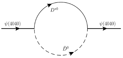
Figure 1: Example of one-loop contribution. Here the case of $D^{\ast 0}$ and $\bar{D}^{0}$ is shown.

The spectral function is connected to the imaginary part of the propagator introduced above as

$$d_{\psi}(m)=\frac{2m}{\pi}\left|\operatorname{Im}\Delta_{\psi}(p^{2}=m^{2})\right|\text{ .}$$ (18)

The quantity $d_{\psi}(m)\mathrm{dm}$ determines the probability that the state $\psi(4040)$ has a mass between $m$ and $m+\mathrm{dm}$. It must fulfill the normalization condition

$$\int\limits_{0}^{\infty}d_{\psi}(m)\mathrm{dm}=1\text{ .}$$ (19)

The validity of the normalization is a crucial feature of our study, since it guarantees unitarity [33]. It is a consequence of our theoretical approach (for a detailed mathematical proof of its validity, see Ref. [34]). Note, in Eq. (19) the integration is up to $m\rightarrow\infty$ (hence, $k\rightarrow\infty,$ see Eq. (8)). In practice, we shall verify numerically that Eq. (19) is fulfilled (we do so by integrating up to $10$ GeV, far above the region of interest of about 4 GeV).

In addition, the partial spectral functions read:

$$d_{\psi\rightarrow DD}(m) =\frac{2m}{\pi}\left|\Delta_{\psi}(m^{2})\right|^{2}m\Gamma_{\psi(4040)\rightarrow DD}(m)\text{ ,}$$ (20)

$$d_{\psi\rightarrow D_{s}^{+}D_{s}^{-}}(m) =\frac{2m}{\pi}\left|\Delta_{\psi}(m^{2})\right|^{2}m\Gamma_{\psi(4040)\rightarrow D_{s}D_{s}}(m)\text{ ,}$$ (21)

$$d_{\psi\rightarrow DD^{\ast}}(m) =\frac{2m}{\pi}\left|\Delta_{\psi}(m^{2})\right|^{2}m\Gamma_{\psi(4040)\rightarrow DD^{\ast}}(m)\text{ ,}$$ (22)

$$d_{\psi\rightarrow D_{s}^{\ast}D_{s}}(m) =\frac{2m}{\pi}\left|\Delta_{\psi}(m^{2})\right|^{2}m\Gamma_{\psi(4040)\rightarrow D_{s}^{\ast}D_{s}}(m)\text{ ,}$$ (23)

$$d_{\psi\rightarrow D^{\ast}D^{\ast}}(m) =\frac{2m}{\pi}\left|\Delta_{\psi}(m^{2})\right|^{2}m\Gamma_{\psi(4040)\rightarrow D^{\ast}D^{\ast}}(m)\text{ .}$$ (24)

For instance, $d_{\psi\rightarrow DD^{\ast}}(m)\mathrm{dm}$ is the probability that the resonance $\psi(4040)$ has a mass between $m$ and $m+\mathrm{dm}$ and decays in the channel $DD^{\ast}$ [35]. Similar interpretations hold for all other channels. These quantities are physically interesting since they emerge when different channels are studied; if, for instance, the process $e^{+}e^{-}\rightarrow DD^{\ast}$ is considered, the corresponding cross section is proportional to $d_{\psi\rightarrow DD^{\ast}}(m)$.

2.2 Determination of the parameters

Our model contains five free parameters: the three coupling constants $g_{\psi DD}$, $g_{\psi D^{\ast}D}$, $g_{\psi D^{\ast}D^{\ast}}$ entering Eqs. (2), (3), and (4), the bare mass of the vector state $M_{\psi}$ entering in the propagator (11), and the energy scale (cutoff) $\Lambda$ included in Eq. (9) or Eq. (10).

We proceed as follows: first, we fix the value of $\Lambda$ in the range $0.4$-$0.6$ GeV. Then, in order to determine the coupling constants three experimental values are needed. We use the following measured ratios of branching fractions reported in PDG [5] (see also Refs. [13, 36, 37, 38]):

$$\left.\frac{\mathcal{B}(\psi(4040)\rightarrow D\bar{D})}{\mathcal{B}(\psi(4040)\rightarrow D^{\ast}\bar{D})}\right|_{\exp}=0.24\pm 0.05\pm 0.12\text{ ,}$$ (25)

$$\left.\frac{\mathcal{B}(\psi(4040)\rightarrow D^{\ast}\bar{D}^{\ast})}{\mathcal{B}(\psi(4040)\rightarrow D^{\ast}\bar{D})}\right|_{\exp}=0.18\pm 0.14\pm 0.03\text{ ,}$$ (26)

where the first error is statistical and the second is systematic. Moreover, we employ the experimental value of the total width of the $\psi(4040)$ resonance PDG [5]

$$\Gamma_{\psi(4040)}^{\text{tot,exp}}=80\pm 10\hskip 5.69046pt\text{MeV .}$$ (27)

The vector state $\psi(4040)$ decays into various two-body final states. The decay channels contributing mostly to its total decay width are: $DD$, $D_{s}D_{s}$, $D^{\ast}D$, $D_{s}^{\ast}D_{s}$ and $D^{\ast}D^{\ast}$. The corresponding theoretical expression for the total decay width of $\psi(4040)$ state is given by

$$\Gamma_{\psi(4040)}^{\text{tot,theory}}=\Gamma_{\psi(4040)\rightarrow DD}^{\text{on}\hskip 2.84544pt\text{shell}}+\Gamma_{\psi(4040)\rightarrow D_{s}D_{s}}^{\text{on}\hskip 2.84544pt\text{shell}}+\Gamma_{\psi(4040)\rightarrow D^{\ast}D}^{\text{on}\hskip 2.84544pt\text{shell}}+\Gamma_{\psi(4040)\rightarrow D_{s}^{\ast}D_{s}}^{\text{on}\hskip 2.84544pt\text{shell}}+\Gamma_{\psi(4040)\rightarrow D^{\ast}D^{\ast}}^{\text{on}\hskip 2.84544pt\text{shell}}\text{ ,}$$ (28)

where “on-shell” means that the physical PDG mass $m=4.04$ GeV is employed.

Finally, the coupling constants $g_{\psi DD}$, $g_{\psi D^{\ast}D}$ and $g_{\psi D^{\ast}D^{\ast}}$ as well as their errors are obtained upon minimizing the $\chi^{2}$ function $F_{E}$ depending on all this three parameters:

$$F_{E}(g_{\psi DD},g_{\psi D^{\ast}D},g_{\psi D^{\ast}D^{\ast}}) =\left(\frac{\frac{\Gamma_{\psi\rightarrow DD}^{theory}(g_{\psi DD})}{\Gamma_{\psi\rightarrow D^{\ast}D}^{theory}(g_{\psi D^{\ast}D})}-\left.\frac{\mathcal{B}(\psi(4040)\rightarrow D\bar{D})}{\mathcal{B}(\psi(4040)\rightarrow D^{\ast}\bar{D})}\right|_{\exp}}{\delta\left.\frac{\mathcal{B}(\psi(4040)\rightarrow D\bar{D})}{\mathcal{B}(\psi(4040)\rightarrow D^{\ast}\bar{D})}\right|_{\exp}}\right)^{2}+$$

$$\left(\frac{\frac{\Gamma_{\psi\rightarrow D^{\ast}D^{\ast}}^{theory}(g_{\psi D^{\ast}D^{\ast}})}{\Gamma_{\psi\rightarrow D^{\ast}D}^{theory}(g_{\psi D^{\ast}D})}-\left.\frac{\mathcal{B}(\psi(4040)\rightarrow D^{\ast}\bar{D}^{\ast})}{\mathcal{B}(\psi(4040)\rightarrow D^{\ast}\bar{D})}\right|_{\exp}}{\delta\left.\frac{\mathcal{B}(\psi(4040)\rightarrow D^{\ast}\bar{D}^{\ast})}{\mathcal{B}(\psi(4040)\rightarrow D^{\ast}\bar{D})}\right|_{\exp}}\right)^{2} +\left(\frac{\Gamma_{\psi(4040)}^{tot,theory}(g_{\psi DD},g_{\psi D^{\ast}D},g_{\psi D^{\ast}D^{\ast}})-\Gamma_{\psi(4040)}^{tot,exp}}{\delta\Gamma_{\psi(4040)}^{tot,exp}}\right)^{2}$$ (29)

The bare mass $M_{\psi}$ was fixed under the requirement that the maximum of the spectral function corresponds to the nominal mass of $\psi(4040)$, hence to $4.04$ GeV.

The numerical values of $g_{\psi DD}$, $g_{\psi D^{\ast}D}$, $g_{\psi D^{\ast}D^{\ast}}$ and of bare mass $M_{\psi}$ are reported in Tab. 1 in Sec. 3.1 for given values of the cutoff $\Lambda$. As expected, $g_{\psi D^{\ast}D}$, $g_{\psi D^{\ast}D^{\ast}}$ depend rather mildly on $\Lambda$, but $g_{\psi DD}$ quite strongly. However, the decay width into $DD$ is very small and affects only slightly the overall picture. For completeness, we report in Appendix A also the partial decay widths for various choices of the cutoff and for different form factors. While the results are basically compatible with each other, future experimental determination of the channel $\psi(4040)\rightarrow D_{s}^{+}D_{s}^{-}$ would be very helpful to constrain our model.

3 Results

In this section we show the results and comment on them. First, in Sec. 3.1 we concentrate on the form of the full spectral function (as well as the partial ones into $DD$, $D^{\ast}D$, $D^{\ast}D^{\ast}$ channels) of the resonance $\psi(4040)$. Moreover we determine the position of the pole(s) in the complex plane. Then, in Sec. 3.2 we present the discussion of the important process $e^{+}e^{-}\rightarrow J/\psi\pi^{+}\pi^{-}$ and the possible generation of a peak for $Y(4008)$.

3.1 Spectral function and pole positions

Since scattering data have still quite large errors, it is not yet possible to determine the value of $\Lambda$ through a fit. Moreover, such a fit would also need to include an unknown background contribution. This is why $\Lambda$ has been varied in a quite large range in Table 1, in which the positions of the poles have also been reported. As already mentioned in the introduction, we always find two poles in the complex plane, one corresponding to the maximum of the spectral function and an additional dynamically generated one. For $\Lambda$ up to $\sim 0.5$ GeV similar results are obtained, but for larger values the second pole (even if always present) appears at higher values. We have also tested values larger than $0.6$ GeV, but they do not generate satisfactory results. (This outcome is in agreement with the results of Sec. 3.2 and Appendix B, see later on).

In the following, we choose for the numerical value $\Lambda=0.42,$ since it generates a pole whose imaginary part is $40$ MeV, then $\Gamma_{\psi(4040)}^{\text{pole }}=80$ MeV. We then use this value for illustration and for the presentation of the plots. (Yet, it should not be considered as a sharp value for the cutoff). The spectral function $d_{\psi}(m)$ defined in Eq. (18) is shown in Fig. 2.a together with a standard Breit-Wigner function peaked at $4.04$ GeV and with a width of $80$ MeV, which serves for comparison.

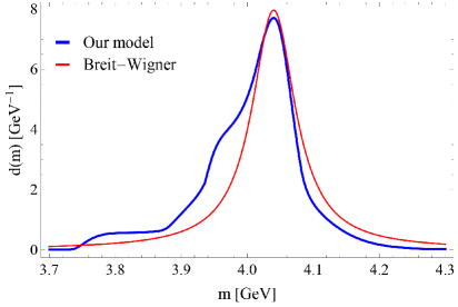
a)

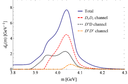
b)

Figure 2: Panel (a) presents the shape of the spectral function of the resonance $\psi(4040)$ of Eq. (18) (blue line) with comparison to the standard Breit-Wigner form (red line). Panel (b) presents the partial spectral functions for $D_{s}D_{s}$, $D^{\ast}D$ and $D^{\ast}D^{\ast}$ channels (This channels are described by Eq. (14), Eq. (15) and Eq. (16)). The corresponding parameters are presented in Table 1.

Only one single peak close to $4.04$ GeV corresponding to the standard seed $\bar{c}c$ state is present. While the Breit-Wigner function approximates quite well the spectral function close to the peak, sizable deviations close to $3.9$ GeV are present. This is due to an enhancement in the energy region below $4$ GeV, which is generated by meson-meson loops.

In Fig. 2.b we present the contributions of individual channels ($DD$, $D^{\ast}D$ and $D^{\ast}D^{\ast}$) to the total spectral function. The $D^{\ast}D$ channel turns out to be the most important for the deformation on the l.h.s. of the spectral function. In the complex plane we found two poles: one for $4.053-0.039$ $i$ GeV, corresponding to $\psi(4040)$ resonance, and one for $3.934-0.030$ $i$ GeV. Thus, even if only one single seed state identified with $\psi(4040)$ was included into the calculations, two poles naturally emerge.

At a first sight, it is tempting to identify the additional pole with the controversial state $Y(4008).$ Moreover, a look at Table 1 shows that a second additional pole always exists, and up to values of about $0.5$ GeV the dynamically generated pole is not far from $4$ GeV. However, care is needed for the following reasons: the pole width of the additional state is too small when compared to the experimental value (about $200$ MeV), but it should be stressed that a direct comparison of this pole width and the experiment is misleading, since very different reactions were measured, see later on. If the enhancement in Fig. 1 is real, it should be visible in the cross-section of the channel $e^{+}e^{-}\rightarrow\psi(4040)\rightarrow D^{\ast}D,$ which is proportional to $d_{\psi\rightarrow DD^{\ast}}(m)$ (see Fig. 1.b); presently, the data have too large errors to resolve such a complicated structure. Quite importantly, the state $Y(4008)$ has been observed in the ISR reaction $e^{+}e^{-}\rightarrow\gamma e^{+}e^{-}\rightarrow\gamma\pi^{+}\pi^{-}J/\psi$ and not in the $DD^{\ast}$ channel, see next section for the discussion of this important point.

	Gaussian form factor		Dipolar form factor
$\Lambda$	Parameters	Pole(s) [GeV]	Parameters	Pole(s) [GeV]
0.4	$g_{\psi DD}=48.8\pm 4.6$	$\bullet\hskip 8.5359pt(4.052\pm 0.003)$	$g_{\psi DD}=25.4\pm 5.0$	$\bullet\hskip 8.5359pt(4.058\pm 0.019)$
	$g_{\psi D^{*}D}=3.60\pm 0.95$	$\hskip 8.5359pt-i(0.035\pm 0.005)$	$g_{\psi D^{*}D}=3.50\pm 0.58$	$\hskip 8.5359pt-i(0.050\pm 0.014)$
	$g_{\psi D^{*}D^{*}}=1.65\pm 0.86$	$\blacklozenge\hskip 8.5359pt(3.936\pm 0.005)$	$g_{\psi D^{*}D^{*}}=1.93\pm 0.89$	$\blacklozenge\hskip 8.5359pt(3.941\pm 0.003)$
	$M_{\psi}=4.00$	$\hskip 8.5359pt-i(0.022\pm 0.001)$	$M_{\psi}=4.02$	$\hskip 8.5359pt-i(0.045\pm 0.010)$
0.42	$g_{\psi DD}=39.8\pm 5.0$	$\bullet\hskip 8.5359pt(4.053\pm 0.004)$	$g_{\psi DD}=21.7\pm 4.4$	$\bullet\hskip 8.5359pt(4.062\pm 0.023)$
	$g_{\psi D^{*}D}=3.44\pm 0.80$	$\hskip 8.5359pt-i(0.039\pm 0.009)$	$g_{\psi D^{*}D}=3.06\pm 0.49$	$\hskip 8.5359pt-i(0.056\pm 0.011)$
	$g_{\psi D^{*}D^{*}}=1.85\pm 0.93$	$\blacklozenge\hskip 8.5359pt(3.934\pm 0.006)$	$g_{\psi D^{*}D^{*}}=1.94\pm 0.89$	$\blacklozenge\hskip 8.5359pt(3.942\pm 0.004)$
	$M_{\psi}=4.01$	$\hskip 8.5359pt-i(0.030\pm 0.001)$	$M_{\psi}=4.03$	$\hskip 8.5359pt-i(0.052\pm 0.010)$
0.45	$g_{\psi DD}=29.9\pm 5.0$	$\bullet\hskip 8.5359pt(4.055\pm 0.005)$	$g_{\psi DD}=17.4\pm 3.8$	$\bullet\hskip 8.5359pt(4.070\pm 0.027)$
	$g_{\psi D^{*}D}=3.14\pm 0.61$	$\hskip 8.5359pt-i(0.047\pm 0.018)$	$g_{\psi D^{*}D}=2.57\pm 0.38$	$\hskip 8.5359pt-i(0.066\pm 0.008)$
	$g_{\psi D^{*}D^{*}}=2.07\pm 0.99$	$\blacklozenge\hskip 8.5359pt(3.928\pm 0.008)$	$g_{\psi D^{*}D^{*}}=1.97\pm 0.89$	$\blacklozenge\hskip 8.5359pt(3.943\pm 0.006)$
	$M_{\psi}=4.02$	$\hskip 8.5359pt-i(0.042\pm 0.002)$	$M_{\psi}=4.04$	$\hskip 8.5359pt-i(0.064\pm 0.011)$
0.5	$g_{\psi DD}=19.5\pm 4.2$	$\bullet\hskip 8.5359pt(4.055\pm 0.009)$	$g_{\psi DD}=12.6\pm 3.0$	$\bullet\hskip 8.5359pt(4.087\pm 0.033)$
	$g_{\psi D^{*}D}=2.64\pm 0.39$	$\hskip 8.5359pt-i(0.066\pm 0.054)$	$g_{\psi D^{*}D}=2.02\pm 0.27$	$\hskip 8.5359pt-i(0.083\pm 0.006)$
	$g_{\psi D^{*}D^{*}}=2.3\pm 1.0$	$\blacklozenge\hskip 8.5359pt(3.918\pm 0.007)$	$g_{\psi D^{*}D^{*}}=2.02\pm 0.89$	$\blacklozenge\hskip 8.5359pt(3.943\pm 0.011)$
	$M_{\psi}=4.04$	$\hskip 8.5359pt-i(0.063\pm 0.004)$	$M_{\psi}=4.05$	$\hskip 8.5359pt-i(0.085\pm 0.014)$
0.6	$g_{\psi DD}=10.4\pm 2.7$	$\bullet\hskip 8.5359pt(4.025\pm 0.015)$	$g_{\psi DD}=7.4\pm 2.0$	$\bullet\hskip 8.5359pt(4.032\pm 0.019)$
	$g_{\psi D^{*}D}=1.95\pm 0.22$	$\hskip 8.5359pt-i(0.041\pm 0.031)$	$g_{\psi D^{*}D}=1.44\pm 0.16$	$\hskip 8.5359pt-i(0.035\pm 0.020)$
	$g_{\psi D^{*}D^{*}}=2.3\pm 1.0$	$\blacklozenge\hskip 8.5359pt(4.056\pm 0.017)$	$g_{\psi D^{*}D^{*}}=2.09\pm 0.90$	$\blacklozenge\hskip 8.5359pt(4.056\pm 0.023)$
	$M_{\psi}=4.07$	$\hskip 8.5359pt-i(0.032\pm 0.007)$	$M_{\psi}=4.08$	$\hskip 8.5359pt-i(0.029\pm 0.006)$

Table 1: Position of the poles in the complex plane for different parameters used in the model. The coupling constants $g_{\psi DD}$ and $g_{\psi D^{\ast}D^{\ast}}$ are dimensionless, $g_{\psi D^{\ast}D}$ has dimensions GeV^-1, $\Lambda$ and $M_{\psi}$ are in GeV.

Next, we perform a large-$N_{c}$ study of the resonance $\psi(4040)$ (where $N_{c}$ refers to the number of colors in QCD). To this end, we introduce the scaling parameter $\lambda\in(0,1)$, linked to $N_{c}$ as $\lambda=3/N_{c}$, and consider the scaling of the coupling constants as [39]

$$g_{\psi DD}\rightarrow\sqrt{\lambda}g_{\psi DD}\text{ , }g_{\psi D^{\ast}D}\rightarrow\sqrt{\lambda}g_{\psi D^{\ast}D}\text{ , }g_{\psi D^{\ast}D^{\ast}}\rightarrow\sqrt{\lambda}g_{\psi D^{\ast}D^{\ast}}\text{ }.$$ (30)

Clearly, by setting $\lambda=1$, we reobtain our physical results. In the opposite limiting case, $\lambda=0$, the spectral function reduced to a delta function centered in the seed mass, $\delta(m-M_{\psi})$. In Fig. 3 we test the intermediate values $\lambda=0.8,0.6$ and $0.4$ for both the spectral function and the positions of the poles (for the latter, $\lambda=0.5$ is also shown).

a)

b)

Figure 3: Study of the changing of the spectral function (panel a) and pole movement in the complex plane (panel b) for different values of $\lambda$. The used parameters for the plots are: $g_{\psi DD}=39.84$, $g_{\psi D^{\ast}D}=3.44$ GeV^-1, $g_{\psi D^{\ast}D^{\ast}}=1.85$, $M_{\psi}=4.007$ GeV and Gaussian form factor $F_{\Lambda}$ with $\Lambda=0.42$ GeV.

The large-$N_{c}$ study shows that for smaller $\lambda$ (hence, larger $N_{c}$), the left enhancement in the spectral function becomes smaller and finally disappears, while the spectral function becomes narrower. For what concerns the pole trajectory, the seed pole corresponding to $\psi(4040)$ resonance moves towards to real energy axis, while the additional companion pole moves away from it. This behavior confirm that the resonance $\psi(4040)$ is a conventional $q\bar{q}$ meson while the second pole is dynamically generated.

As a last point, we comment on mixing with other vector state, in particular with the closest quarkonium state $\psi(4160).$ By studying the mix propagator (see Refs. [40, 41] for some formal equation), we tested how the spectral function of $\psi(4040)$ changes when taking into account the processes $\psi(4040)\rightarrow DD^{\ast}$ $\rightarrow\psi(4160)\rightarrow DD^{\ast}\rightarrow\psi(4040)$ (this is so because $\psi(4160)$ also couples to $DD^{*}$; analogous processes with  $DD$ and $D^{\ast}D^{\ast}$ are possible). The spectral function of $\psi(4040)$ turns out to be only slightly affected in the region of interest, thus the results here presented would hold also in the enlarged scenario in which more $\bar{c}c$ states are considered.

3.2 Decay into $J/\psi\pi^{+}\pi^{-}$

An important decay channel, in which various $Y$ states have been observed, among which the $Y(4008)$ state is one, is the $e^{+}e^{-}\rightarrow\gamma J/\psi\pi^{+}\pi^{-}$ decay, where the photon $\gamma$ comes from ISR. Hence, the reaction may be recasted into two steps: $e^{+}e^{-}\rightarrow\gamma\left(e^{+}e^{-}\right)_{\text{off-shell}}$ and $\left(e^{+}e^{-}\right)_{\text{off-shell}}\rightarrow J/\psi\pi^{+}\pi.\$

Since the very same fundamental process is involved, for simplicity we consider in the following the process $e^{+}e^{-}\rightarrow J/\psi\pi^{+}\pi^{-}$ (we thus ignore that the electron-positron pair is off-shell). In particular, we are interested in the case in which $\psi(4040)$ is an intermediate state of the reaction

$$e^{+}e^{-}\rightarrow\psi(4040)\rightarrow J/\psi\pi^{+}\pi^{-}\text{ .}$$ (31)

There are basically two ways in which this process can take place. The first one involves the emission of two gluons

$$\psi(4040)\equiv c\bar{c}\rightarrow c\bar{c}+gg\rightarrow J/\psi+f_{0}(500)\rightarrow J/\psi+\pi^{+}\pi^{-}$$ (32)

The choice of $f_{0}(500)$ (see [42] for a review) as an intermediate state is motivated by the fact that it is the lightest quantum state with quantum numbers of the vacuum and is in the right kinematic region ($f_{0}(980)$ is at the border, $f_{0}(1370)$ already too heavy). Nevertheless, one can repeat the very same discussion by considering different $f_{0}$ states. This decay mode can be modelled by

$$\mathcal{L}_{\psi jf_{0}}^{direct}=g_{\psi jf_{0}}^{direct}\psi_{\mu}j^{\mu}f_{0}\text{ ,}$$ (33)

where $j^{\mu}$ is the field corresponding to the $J/\psi$ and $f_{0}$ to $f_{0}(500).$ This term would generate a peak at $4.04$ GeV, which has not been seen experimentally (in fact, this would be a “standard” decay of $\psi(4040)$ peaked at its Breit-Wigner mass). It means that $g_{\psi jf_{0}}^{direct}$ should be quite small. We will neglect this channel in the following.

There is, however, a second mechanism

$$\psi(4040)\rightarrow DD^{\ast}\rightarrow J/\psi+f_{0}(500)\rightarrow J/\psi+\pi^{+}\pi^{-},$$ (34)

where the additional vertex is represented by the following four-body interaction

$$\mathcal{L}_{DD^{\ast}jf_{0}}=\lambda_{DD^{\ast}jf_{0}}\left[\partial^{\mu}D^{\ast+\nu}D^{-}+\partial^{\mu}D^{\ast 0\nu}\bar{D}^{0}\right]j_{\mu\nu}f_{0}\text{ ,}$$ (35)

where $j_{\mu\nu}=\partial_{\mu}j_{\nu}-\partial_{\nu}j_{\mu}.$

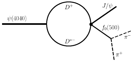
Figure 4: Schematic diagram of the decay $\psi(4040)\rightarrow\pi^{+}\pi^{-}J/\psi$ via $D^{+}D^{\ast-}$ loop.

The spectral function in the channel $J/\psi\pi^{+}\pi^{-}$ reads

$$d_{\psi(4040)\rightarrow J/\psi\pi^{+}\pi^{-}}(m)=\frac{2m}{\pi}\left|\Delta_{\psi}(m^{2})\right|^{2}m\Gamma_{\psi(4040)\rightarrow J/\psi\pi^{+}\pi^{-}}(m)$$ (36)

where

$$\Gamma_{\psi(4040)\rightarrow J/\psi f_{0}(500)}(m)$$

$$=\left|g_{\psi jf_{0}}^{direct}+\lambda_{DD^{\ast}jf_{0}}g_{DD^{\ast}}\left[\Sigma_{D^{0}D^{\ast 0}}(m^{2})+\Sigma_{D^{+}D^{\ast-}}(m^{2})\right]\right|^{2}\frac{k}{8\pi m^{2}}\left(3+\frac{k^{2}}{m_{J/\psi}^{2}}\right)e^{-2\frac{k^{2}}{\Lambda^{2}}}\text{ .}$$ (37)

with $k\equiv k(m,m_{J/\psi},m_{f_{0}(500)}).$ It is then clear that the $DD^{\ast}$ loop, together with the Lagrangian $\mathcal{L}_{DD^{\ast}jf_{0}}$ of Eq. (35), generates a mass-dependent coupling for the channel $\psi(4040)\rightarrow J/\psi f_{0}(500)$.

In general, this decay is small, since both mechanisms are small [they are suppressed (at least) as $1/N_{c}^{3/2}$ in the large-$N_{c}$ limit], yet the second mechanism is expected to be dominant in our case. Namely, the seed state $\psi(4040)$ couples strongly to $D^{\ast}D$ (this is the dominant decay mode). Moreover, the real part of the $DD^{\ast}$ loops, depicted in Fig. 5.a, has a pronounced peak at $m_{D}+m_{D^{\ast}}$ at about $3.9$ GeV. The transition $D^{\ast}D\rightarrow J/\psi f_{0}(500)$ via the Lagrangian $\mathcal{L}_{DD^{\ast}jf_{0}}$ is rather natural, since it implies a redistribution of already existing quarks. Moreover, $f_{0}(500)$ couples strongly to $\bar{u}u$ and $\bar{d}d.$ Hence, in first approximation we shall neglect $g_{\psi jf_{0}}^{direct}$ in the following.

Summarizing, in Eq. (36) the product of two functions is present: $\left|\Delta_{\psi}(m^{2})\right|^{2},$ peaked at $4.04$ GeV, and $\Gamma_{\psi(4040)\rightarrow J/\psi f_{0}(500)}(m),$ peaked at $3.9$ GeV. Of course, other channels, such as $DD,$ would also couple $J/\psi f_{0}(500)$, but (i) the coupling of $\psi(4040)$ to $DD$ is sizably smaller and (ii) the function $\left|\Sigma_{DD}(m^{2})\right|^{2}$ is peaked at the $DD$ threshold, hence the overlap with $\left|\Delta_{\psi}(m^{2})\right|^{2}$ is negligible.

a)

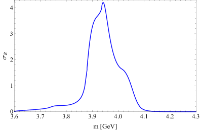
b)

Figure 5: Left panel: $\operatorname{Re}\Sigma_{D^{0\ast}D^{0\ast}}$ and $\operatorname{Re}\Sigma_{D^{+\ast}D^{-\ast}}$ as function of $m.$ Both of them have a peak at about $3.9$ GeV. Right panel: Plot of the (normalized) cross-section $\sigma_{R}(m)$ of the channel $e^{+}e^{-}\rightarrow\psi(4040)\rightarrow J/\psi\pi^{+}\pi^{-}$ deifned in Eq. (39). A deformed and broad structure with a peak at about 3.95 GeV is visible.

For $\sqrt{s}$ in the region of interest, we have

$$\sigma_{e^{+}e^{-}\rightarrow\psi(4040)\rightarrow J/\psi\pi^{+}\pi^{-}}\left(m\right)=\frac{2\pi}{m}g_{\psi e^{+}e^{-}}^{2}d_{\psi(4040)\rightarrow J/\psi\pi^{+}\pi^{-}}(m)\text{ .}$$ (38)

In Fig. 5.b we plot

$$\sigma_{R}(m)=\frac{\sigma_{e^{+}e^{-}\rightarrow\psi(4040)\rightarrow J/\psi\pi^{+}\pi^{-}}\left(m\right)}{\sigma_{e^{+}e^{-}\rightarrow\psi(4040)\rightarrow J/\psi\pi^{+}\pi^{-}}\left(m=m_{D^{0}}+m_{D^{\ast 0}}\right)}.$$ (39)

(In this way, the dependence on the unknown coupling $\lambda_{DD^{\ast}jf_{0}}$ cancels and $\sigma_{R}(m_{D^{0}}+m_{D^{\ast 0}})=1$). The resulting form is quite peculiar and is definitely not a simple Breit-Wigner peak. If the experimental accuracy is not high enough, one may identify this signal as a broad resonance whose peak is centered at about $4$ GeV. Thus, we suggest that the ‘state’ $Y(4008)$ is a manifestation of the standard state $\psi(4040),$ which arises due to the decay into $J/\psi\pi^{+}\pi^{-}$ through the nearby $DD^{\ast}$ loop. It is important to stress that this conclusion is independent of the presence of a dynamically generated pole and its precise position, but it is a consequence of the strong coupling to $DD^{\ast}$ and the fact that the  $DD^{\ast}$ threshold is not far from the peak of $\psi(4040)$.

This mechanism for the generation of the state $Y(4008)$ does not necessarily correspond to a resonance. Moreover, the width of the dynamical pole is not related to the width of the signal of Fig. 5.b. In Appendix B we also present the results for variations of the parameters, and for a cutoff up to $0.5$ GeV a very similar outcome is obtained.

4 Summary and discussion

We studied the energy region close to the resonance $\psi(4040)$ in the framework of a QFT effective model. We evaluated its spectral function and found that, besides the expected resonance pole of $\psi(4040)$ (corresponding to peak in the spectral function and to the underlying seed $c\bar{c}$ state), an additional companion pole (no peak, but an enhancement in the spectral function) emerges naturally within our approach (see Table 1). Illustrative result in agreement with phenomenology are: $4.053-i0.039$ GeV for the seed state $\psi(4040)$ and $3.934-i0.030$ GeV for the enhancement. A large-$N_{c}$ study confirms that $\psi(4040)$ resonance is predominantly a charm-anticharm state, while the second pole is dynamically generated by meson-meson quantum fluctuations.

The pole itself cannot be directly associated to the $Y(4008).\$Namely, this pole would be mostly visible in a two-peak structure of the cross-section $e^{+}e^{-}\rightarrow\psi(4040)\rightarrow DD^{\ast}$ (whose data precision is not good enough). Yet, the chain $e^{+}e^{-}\rightarrow\psi(4040)\rightarrow DD^{\ast}\rightarrow J/\psi+f_{0}(500)\rightarrow J/\psi\pi^{+}\pi^{-}$is quite promising: the $DD^{\ast}$ loop generates a peak at about $3.9$ GeV in the cross-section. The strong coupling of $\psi(4040)$ to $DD^{\ast}$ and the overlap of the $DD^{\ast}$-loop function with the modulus square of the propagator are responsible for a quite broad peak in the corresponding spectral function, which can be identified with $Y(4008)$. The important point is that the existence of an additional pole corresponding to $Y(4008)$ is possible (and indeed it does exist for the parameters of our model) but is actually not necessary for the process that we describe. The very same mechanism can be also investigated in the future in other channels, as for instance in connection with the states $Y(4260)$ and $\psi(4160)$.

Acknowledgements The authors thank S. Coito for useful discussions. M.P. and F.G. acknowledge financial support from the Polish National Science Centre (NCN) through the OPUS project no. 2015/17/B/ST2/01625. P. K. were supported by the Hungarian OTKA fund K109462 and by the ExtreMe Matter Institute EMMI at the GSI Helmholtzzentrum fur Schwerionenforschung, Darmstadt, Germany.

Appendix A Decay widths on shell

Here we present the results for the on-shell decay widths for both form factors and for different values of the cutoff, respectively. Even if the qualitative picture does not change much, one observes non-negligible variations of the partial decay widths as function of the cutoff $\Lambda.$ In the future, a better determination of the decay $\psi(4040)$ into $D_{s}^{+}D_{s}^{-}$ (presently only seen) would constitute a useful constraint on our model.

		Partial decay width [MeV]
$\mathbf{\Lambda}$ [GeV]	Decay channel	Gaussian form factor	Dipolar form factor
	$DD$	$4.24\pm 0.80$	$8.8\pm 3.5$
	$D_{s}D_{s}$	$55\pm 10$	$28\pm 11$
0.4	$D^{*}D$	$17.7\pm 9.3$	$37\pm 12$
	$D^{*}_{s}D_{s}$	$0$	$0$
	$D^{*}D^{*}$	$3.2_{-3.2}^{+3.3}$	$6.6\pm 6.1$
	$DD$	$5.6\pm 1.4$	$9.2\pm 3.8$
	$D_{s}D_{s}$	$47\pm 12$	$26\pm 10$
0.42	$D^{*}D$	$23\pm 11$	$38\pm 12$
	$D^{*}_{s}D_{s}$	$0$	$0$
	$D^{*}D^{*}$	$4.2^{+4.3}_{-4.2}$	$6.9\pm 6.3$
	$DD$	$7.5\pm 2.5$	$9.8\pm 4.2$
	$D_{s}D_{s}$	$35\pm 12$	$22.2\pm 9.6$
0.45	$D^{*}D$	$31\pm 12$	$41\pm 12$
	$D^{*}_{s}D_{s}$	$0$	$0$
	$D^{*}D^{*}$	$5.7\pm 5.4$	$7.3\pm 6.6$
	$DD$	$9.8\pm 4.2$	$10.7\pm 5.0$
	$D_{s}D_{s}$	$22.2\pm 9.6$	$17.0\pm 8.0$
0.5	$D^{*}D$	$41\pm 12$	$44\pm 12$
	$D^{*}_{s}D_{s}$	$0$	$0$
	$D^{*}D^{*}$	$7.3\pm 6.6$	$8.0\pm 7.1$
	$DD$	$11.8\pm 6.2$	$11.9\pm 6.3$
	$D_{s}D_{s}$	$10.4\pm 5.4$	$9.6\pm 5.1$
0.6	$D^{*}D$	$49\pm 11$	$50\pm 11$
	$D^{*}_{s}D_{s}$	$0$	$0$
	$D^{*}D^{*}$	$8.8\pm 7.6$	$8.9\pm 7.7$

Table 2: Partial decay widths on-shell for both types of form factor and different values of $\Lambda$ parameter.

Appendix B Decay into $J/\psi\pi^{+}\pi^{-}$ - variations of the parameter $\Lambda$

As it was discussed in the paper, the decay of $\psi(4040)$ into $J/\psi\pi^{+}\pi^{-}$ via $DD^{\ast}$ loops generates a sizable peak in the cross-section in the energy region close to $4$ GeV. This is an important aspect of our theoretical framework, thus we present in Fig. 6 how the results of the cross-section of Eq. (39) depend on the different values of cutoff.

Figure 6: Study of the cross-section ratio of Eq. (39) upon changing the value of cutoff parameter.

When $\Lambda$ varies in the range from $0.38$ up to (at most) $0.5$ GeV one observes a broad peak at about $3.95$ GeV. For $\Lambda=0.5$ one has actually a quite broad structure, but the peak is already at bout 4.04 GeV. For larger values of $\Lambda$, there is a single peak close to $4.04$ GeV which corresponds to standard $c\bar{c}$ seed state $\psi(4040)$. Hence, for the generation of a signal resembling $Y(4008)$ the value of $\Lambda$ should not exceed $0.5$ GeV.

References

- [1] N. Brambilla et al., “Heavy quarkonium: progress, puzzles, and opportunities,” Eur. Phys. J. C 71 (2011) 1534 doi:10.1140/epjc/s10052-010-1534-9 [arXiv:1010.5827 [hep-ph]].
- [2] H. X. Chen, W. Chen, X. Liu and S. L. Zhu, “The hidden-charm pentaquark and tetraquark states,” Phys. Rept. 639 (2016) 1 doi:10.1016/j.physrep.2016.05.004 [arXiv:1601.02092 [hep-ph]].
- [3] A. Esposito, A. L. Guerrieri, F. Piccinini, A. Pilloni and A. D. Polosa, “Four-Quark Hadrons: an Updated Review,” Int. J. Mod. Phys. A 30 (2015) 1530002 doi:10.1142/S0217751X15300021 [arXiv:1411.5997 [hep-ph]].
- [4] M. Nielsen, F. S. Navarra and S. H. Lee, “New Charmonium States in QCD Sum Rules: A Concise Review,” Phys. Rept. 497 (2010) 41 doi:10.1016/j.physrep.2010.07.005 [arXiv:0911.1958 [hep-ph]].
- [5] M. Tanabashi et al. (Particle Data Group), Phys. Rev. D 98, 030001 (2018) doi:10.1103/PhysRevD.98.030001
- [6] S. Godfrey and N. Isgur, “Mesons in a Relativized Quark Model with Chromodynamics,” Phys. Rev. D 32 (1985) 189. doi:10.1103/PhysRevD.32.189
- [7] E. Eichten, K. Gottfried, T. Kinoshita, K. D. Lane and T. M. Yan, “Charmonium: The Model”, Phys. Rev. D 17 (1978) 3090 Erratum: [Phys. Rev. D 21 (1980) 313]. doi:10.1103/PhysRevD.17.3090, 10.1103/physrevd.21.313.2 E. Eichten, K. Gottfried, T. Kinoshita, K. D. Lane and T. M. Yan, “Charmonium: Comparison with Experiment”, Phys. Rev. D 21 (1980) 203. doi:10.1103/PhysRevD.21.203 E. Eichten, K. Gottfried, T. Kinoshita, K. D. Lane and T. M. Yan, Phys. Rev. Lett. 36 (1976) 500. doi:10.1103/PhysRevLett.36.500
- [8] J. Segovia, D. R. Entem, F. Fernandez and E. Hernandez, “Constituent quark model description of charmonium phenomenology,” Int. J. Mod. Phys. E 22 (2013) 1330026 doi:10.1142/S0218301313300269 [arXiv:1309.6926 [hep-ph]].
- [9] P. G. Ortega, J. Segovia, D. R. Entem and F. Fernández, “Charmonium resonances in the 3.9 GeV/ energy region and the puzzle,” Phys. Lett. B 778 (2018) 1 doi:10.1016/j.physletb.2018.01.005 [arXiv:1706.02639 [hep-ph]].
- [10] C. Z. Yuan et al. [Belle Collaboration], “Measurement of e+ e- — pi+ pi- J/psi cross-section via initial state radiation at Belle,” Phys. Rev. Lett. 99 (2007) 182004 doi:10.1103/PhysRevLett.99.182004 [arXiv:0707.2541 [hep-ex]].
- [11] Z. Q. Liu et al. [Belle Collaboration], “Study of and Observation of a Charged Charmoniumlike State at Belle,” Phys. Rev. Lett. 110 (2013) 252002 doi:10.1103/PhysRevLett.110.252002 [arXiv:1304.0121 [hep-ex]].
- [12] X. Y. Gao, C. P. Shen and C. Z. Yuan, “Resonant parameters of the ,” Phys. Rev. D 95 (2017) no.9, 092007 doi:10.1103/PhysRevD.95.092007 [arXiv:1703.10351 [hep-ex]].
- [13] B. Aubert et al. [BaBar Collaboration], “Exclusive Initial-State-Radiation Production of the D anti-D, D* anti-D*, and D* anti-D* Systems,” Phys. Rev. D 79 (2009) 092001 doi:10.1103/PhysRevD.79.092001 [arXiv:0903.1597 [hep-ex]].
- [14] M. Ablikim et al. [BESIII Collaboration], “Precise measurement of the cross section at center-of-mass energies from 3.77 to 4.60 GeV,” Phys. Rev. Lett. 118 (2017) no.9, 092001 doi:10.1103/PhysRevLett.118.092001 [arXiv:1611.01317 [hep-ex]].
- [15] X. Liu, “Understanding the newly observed Y(4008) by Belle,” Eur. Phys. J. C 54 (2008) 471 doi:10.1140/epjc/s10052-008-0551-4 [arXiv:0708.4167 [hep-ph]].
- [16] W. Xie, L. Q. Mo, P. Wang and S. R. Cotanch, “Coulomb gauge model for hidden charm tetraquarks,” Phys. Lett. B 725 (2013) 148 doi:10.1016/j.physletb.2013.07.003 [arXiv:1302.5737 [hep-ph]].
- [17] G. J. Ding, “Bound States of the Heavy Flavor Vector Mesons and Y(4008) and Z+(1)(4050),” Phys. Rev. D 80 (2009) 034005 doi:10.1103/PhysRevD.80.034005 [arXiv:0905.1188 [hep-ph]].
- [18] L. Maiani, F. Piccinini, A. D. Polosa and V. Riquer, “The Z(4430) and a New Paradigm for Spin Interactions in Tetraquarks,” Phys. Rev. D 89 (2014) 114010 doi:10.1103/PhysRevD.89.114010 [arXiv:1405.1551 [hep-ph]].
- [19] P. Zhou, C. R. Deng and J. L. Ping, “Identification of Y (4008), Y (4140), Y (4260), and Y (4360) as Tetraquark States,” Chin. Phys. Lett. 32 (2015) no.10, 101201. doi:10.1088/0256-307X/32/10/101201
- [20] D. Y. Chen, X. Liu, X. Q. Li and H. W. Ke, “Unified Fano-like interference picture for charmoniumlike states Y(4008), Y(4260) and Y(4360),” Phys. Rev. D 93 (2016) 014011 doi:10.1103/PhysRevD.93.014011 [arXiv:1512.04157 [hep-ph]].
- [21] B. Q. Li and K. T. Chao, “Higher Charmonia and X,Y,Z states with Screened Potential,” Phys. Rev. D 79 (2009) 094004 doi:10.1103/PhysRevD.79.094004 [arXiv:0903.5506 [hep-ph]].
- [22] L. J. Chen, D. D. Ye and A. Zhang, “Is possibly a state?,” Eur. Phys. J. C 74 (2014) no.8, 3031 doi:10.1140/epjc/s10052-014-3031-z [arXiv:1402.5470 [hep-ph]].
- [23] E. van Beveren, T. A. Rijken, K. Metzger, C. Dullemond, G. Rupp and J. E. Ribeiro, “A Low Lying Scalar Meson Nonet in a Unitarized Meson Model,” Z. Phys. C 30 (1986) 615 doi:10.1007/BF01571811 [arXiv:0710.4067 [hep-ph]].
- [24] N. A. Tornqvist, “Understanding the scalar meson q anti-q nonet,” Z. Phys. C 68 (1995) 647 doi:10.1007/BF01565264 [hep-ph/9504372].
- [25] M. Boglione and M. R. Pennington, “Dynamical generation of scalar mesons,” Phys. Rev. D 65 (2002) 114010 doi:10.1103/PhysRevD.65.114010 [hep-ph/0203149].
- [26] T. Wolkanowski, F. Giacosa and D. H. Rischke, “ revisited,” Phys. Rev. D 93 (2016) no.1, 014002 doi:10.1103/PhysRevD.93.014002 [arXiv:1508.00372 [hep-ph]].
- [27] T. Wolkanowski, M. Soltysiak and F. Giacosa, “ as a companion pole of ,” Nucl. Phys. B 909 (2016) 418 . doi:10.1016/j.nuclphysb.2016.05.025 [arXiv:1512.01071 [hep-ph]].
- [28] S. Coito and F. Giacosa, “Line-shape and poles of the ,” arXiv:1712.00969 [hep-ph]. S. Coito and F. Giacosa, “Formation and Deformation of the ,” Acta Phys. Polon. Supp. 10 (2017) 1049 doi:10.5506/APhysPolBSupp.10.1049 [arXiv:1708.02041 [hep-ph]].
- [29] J. Terning, Phys. Rev. D 44 (1991) 887. G. V. Efimov and M. A. Ivanov, “The Quark confinement model of hadrons,” Bristol, UK: IOP (1993) 177 p. Y. V. Burdanov, G. V. Efimov, S. N. Nedelko and S. A. Solunin, Phys. Rev. D 54 (1996) 4483 [arXiv:hep-ph/9601344]. A. Faessler, T. Gutsche, M. A. Ivanov, V. E. Lyubovitskij and P. Wang, Phys. Rev. D 68 (2003) 014011 [arXiv:hep-ph/0304031]. F. Giacosa, T. Gutsche and A. Faessler, Phys. Rev. C 71 (2005) 025202 [arXiv:hep-ph/0408085].
- [30] M. Soltysiak and F. Giacosa, “A covariant nonlocal Lagrangian for the description of the scalar kaonic sector,” Acta Phys. Polon. Supp. 9 (2016) 467 doi:10.5506/APhysPolBSupp.9.467 [arXiv:1607.01593 [hep-ph]].
- [31] E. S. Ackleh, T. Barnes and E. S. Swanson, “On the mechanism of open flavor strong decays,’Phys. Rev. D 54 (1996) 6811 doi:10.1103/PhysRevD.54.6811 [hep-ph/9604355].
- [32] Z. G. Luo, X. L. Chen and X. Liu, “B(s1)(5830) and B*(s2)(5840),” Phys. Rev. D 79 (2009) 074020 doi:10.1103/PhysRevD.79.074020 [arXiv:0901.0505 [hep-ph]].
- [33] F. Giacosa and G. Pagliara, “On the spectral functions of scalar mesons,” Phys. Rev. C 76 (2007) 065204 doi:10.1103/PhysRevC.76.065204 [arXiv:0707.3594 [hep-ph]].
- [34] F. Giacosa and G. Pagliara, “Spectral function of a scalar boson coupled to fermions,” Phys. Rev. D 88 (2013) no.2, 025010 doi:10.1103/PhysRevD.88.025010 [arXiv:1210.4192 [hep-ph]].
- [35] F. Giacosa, “Non-exponential decay in quantum field theory and in quantum mechanics: the case of two (or more) decay channels,” Found. Phys. 42 (2012) 1262 doi:10.1007/s10701-012-9667-3 [arXiv:1110.5923 [nucl-th]].
- [36] X. L. Wang et al. [Belle Collaboration], “Observation of and decay into ηJ/,” Phys. Rev. D 87 (2013) no.5, 051101 doi:10.1103/PhysRevD.87.051101 [arXiv:1210.7550 [hep-ex]].
- [37] M. N. Anwar, Y. Lu and B. S. Zou, “Modeling Charmonium- Decays of Higher Charmonia,” Phys. Rev. D 95 (2017) no.11, 114031 doi:10.1103/PhysRevD.95.114031 [arXiv:1612.05396 [hep-ph]].
- [38] T. E. Coan et al. [CLEO Collaboration], “Charmonium decays of Y(4260), psi(4160) and psi(4040),” Phys. Rev. Lett. 96 (2006) 162003 doi:10.1103/PhysRevLett.96.162003 [hep-ex/0602034].
- [39] E. Witten, “Baryons in the 1/n Expansion,” Nucl. Phys. B 160 (1979) 57. doi:10.1016/0550-3213(79)90232-3
- [40] G. V. Baryshevskii, V. I. Lyuboshitz, M .I. Podgorerskii, Nonorthogonal quasisationary states, Soviet Physics JETP, Vol. 30, no. 1, January 1970.
- [41] N.N. Achasov and G.N. Shestakov, Line shape of in , Phys. Rev. D 86, 114013 (2012) doi:10.1103/PhysRevD.86.114013 [arXiv:1208.4240 [hep-ph]].
- [42] J. R. Pelaez, “From controversy to precision on the sigma meson: a review on the status of the non-ordinary resonance,” Phys. Rept. 658 (2016) 1 doi:10.1016/j.physrep.2016.09.001 [arXiv:1510.00653 [hep-ph]].