Low temperature scattering with the R-matrix method: the Morse potential

Abstract

Experiments are starting to probe collisions and chemical reactions between atoms and molecules at ultra-low temperatures. We have developed a new theoretical procedure for studying these collisions using the R-matrix method. Here this method is tested for the atom – atom collisions described by a Morse potential. Analytic solutions for continuum states of the Morse potential are derived and compared with numerical results computed using an R-matrix method where the inner region wavefunctions are obtained using a standard nuclear motion algorithm. Results are given for eigenphases and scattering lengths. Excellent agreement is obtained in all cases. Progress in developing a general procedure for treating ultra-low energy reactive and non-reactive collisions is discussed.

1 Introduction

The ability to perform very low-energy collisions between heavy particles is leading to a quiet revolution at the border between atomic physics and experimental quantum chemistry [1]. Studies of reactive and non-reactive collisions at temperatures very significantly below 1 K are starting to probe processes which are not easily resolved at higher temperatures. These experiments study chemical reactions and scattering at the quantum scattering limit where, asymptotically, only a few partial waves contribute [2].

To address these problems theoretically requires the development of new computational techniques. Recently, we proposed adapting R-matrix theory to the study of ultra-low energy reactive and non-reactive, heavy-particle collisions [3]. R-matrix theory involves the division of space into an inner region encompassing the whole collision complex and an outer region where species involved in the scattering can be separately identified. Procedures based on the computable R-matrix method have proved outstandingly successful for the study of electron collisions with atoms and molecules [4, 5], and are increasingly being adopted in other areas [6]. In the computable R-matrix method, the Schrödinger equation for the restricted inner region is solved once and for all for each scattering symmetry, independent of the precise scattering energy. For heavy particle scattering this procedure is particularly appropriate for reactive or non-reactive collisions which occur over deep potential energy wells. Thus, for example, H + H₂ collisions do not occur over a deep well as the H₃ system is only weakly bound [7], while collisions between H⁺ + H₂ occur over the deep well of the H${}_{3}^{+}$ potential energy surface [8].

Strongly bound systems with deep potential energy wells support many bound states. Even the very lowest continuum states which are associated with ultra-low energy scattering feel the effect of these many bound states which lie below them in energy. The result is that even the lowest scattering state has a complicated wavefunction which couples many channels which are asymptotically closed. It is well-known that this situation leads to a plethora of quasibound states, or resonances, in the near-dissociation region [9, 10, 11, 12, 13]. Use of the R-matrix method allows the region of the deep potential well to be treated using variational nuclear motion programs which are capable of giving highly accurate results for energy-independent problems with complicated wavefunctions [14]. It is then only necessary to treat a few partial waves in the energy-dependent outer region. In this region it may be necessary to propagate solutions to very large interparticle separations [15] and to scan over the many energies necessary to characterise narrow resonances.

At present we are in the process of developing a heavy particle R-matrix scattering code, RmatReact, based on the use of a variety of variational nuclear motion codes in the inner region [16, 17, 18, 19, 20]. Doing this involves developing computational procedures which extend methods of the solutions into the continuum [12, 21, 13]. In particular, the problem must be solved within a finite region and, critically, use basis functions which give reliable amplitudes at the R-matrix boundary. These amplitudes, and the associated inner region energies, are used to construct the scattering energy-dependent R-matrix which links the inner and outer regions [3].

In this paper we report on tests we have performed using our methodology for the Morse oscillator potential. Section 2 gives an overview of the general theory while Section 3 demonstrates that the scattering problem can be solved analytically for a Morse oscillator potential. This allows the rigorous assessment of our numerical procedures, which are discussed in Section 4. Results are given in Section 5, and conclusions and some pointers to our future work are given in the final Section.

2 Theory: The RmatReact method

The theory behind the RmatReact method has been discussed extensively [3, 4, 5], and much of this explanation derives from those discussions. The general principle behind the method is the partitioning of space into an inner and outer region, dependent on the reaction coordinate, as discussed above.

In the case of two atoms colliding there is only one reaction coordinate: the internuclear distance $r$. A point $r=a_{0}$ is defined such that any internuclear distance lower than that is the inner region and any distance larger is the outer region.

Within the inner region, the system is treated as a bound diatom, and the eigenenergies and eigenfunctions of the radial Schrödinger equation with the Morse potential can be determined using software built for nuclear motion calculations. Because the eigenfunctions and values refer to the bound states, they are independent of scattering energy. Likewise, in the outer region, the system is treated as a pair of weakly interacting, unbound atoms. Each atom will have associated atomic channels describing its quantum state.

The inner region was solved in this work using a discrete variable representation (DVR) [22] grid method based on the Lobatto shape functions, which have the property of always having a point defined on both boundaries of the grid. Manolopoulos and Wyatt [23, 24] pioneered the use of these functions for scattering problems. Lobatto shape functions [25] can be used to obtain simple expressions for the components of the Hamiltonian matrix, making it computationally efficient to diagonalise whilst avoiding much of the expensive integration usually involved in constructing a Hamiltonian matrix. Once the inner region has been solved to obtain a diagonalised Hamiltonian matrix, a matrix known as the R-matrix, can be constructed on the boundary $a_{0}$. The R-matrix is constructed from the scattering energy, $E$, the bound eigenenergies, and the values of the eigenfunctions on the boundary $a_{0}$, known as the surface amplitudes.

For a given angular momentum quantum number $J$, if the $m^{\rm{th}}$ surface amplitude associated with the $i^{\rm{th}}$ atomic channel is defined as $w_{im}^{J}(a_{0})$, the $m^{\rm{th}}$ eigenenergy is defined as $E_{m}^{J}$, and the scattering wavefunction for atomic channel $i$ is defined to be $F_{i}^{J}(r,E)$, then the R-matrix has two equivalent definitions at $a_{0}$:

$$F_{i}^{J}(a_{0},E)=\sum_{j=1}^{N_{\rm{ch}}^{J}}a_{0}R_{ij}^{J}(a_{0},E)\frac{dF_{j}^{J}(r,E)}{dr}\bigg{|}_{r=a_{0}},$$ (1)

$$R_{ij}^{J}(a_{0},E)=\frac{\hbar^{2}}{2\mu a_{0}}\sum_{m=1}^{N}\frac{w_{im}^{J}(a_{0})w_{jm}^{J}(a_{0})}{E_{m}^{J}-E},$$ (2)

where the sum in Eq. (1) is over the $N_{\rm{ch}}^{J}$ atomic channels for a given value of $J$ considered in the scattering event, and the sum in Eq. (2) is over the $N$ solutions to the Schrödinger equation within an atomic channel.

In the $J=0$, single channel case considered in this work, $i=j$ and Eq. (1) reduces down to a single term, $N_{\rm{ch}}=1$, and the single R-matrix element is defined as $R(a_{0},E)$. Furthermore, $w_{im}^{J}(a_{0})$ becomes a single surface amplitude, and the sum is over the $N$ surface amplitudes.

As Eq. (1) suggests, the R-matrix can be thought of as the ‘log-derivative’ of the channel function $F^{J}(r,E)$, which is an outer region function. However Eq. (2) shows that the R-matrix can be constructed as a sum over the eigenfunctions and energies of the inner region. The fact that these inner and outer region definitions of the R-matrix are equivalent is what gives the R-matrix method its value: information about the energy-independent inner region provide the starting point for obtaining scattering information.

In the outer region, it is assumed that the potential is small and slowly varying, compared to the deep wells of the inner region. As such, it is possible to use methods which iteratively solve the Schrödinger equations over finite distances to propagate the R-matrix from the boundary at $a_{0}$ to an asymptotic distance $a_{p}$. At $a_{p}$, the potential is assumed to be zero. In this work, the propagation method due to Walker and Light [26, 4] is used.

For the single-channel, the propagation algorithm takes as its input the R-matrix element at the inner region boundary, $R(a_{0},E)$, and produces the R-matrix element at the asymptotic distance, $R(a_{p},E)$. To produce the value of the R-matrix at the outer region point $a_{s}$, $R_{s}(a_{s},E)$, the iteration equation takes as its input the value of the R-matrix at $a_{s-1}$, $R_{s-1}(a_{s-1},E)$, and has the form:

$$R_{s}=\frac{-1}{a_{s}\lambda_{s}}\left(\frac{1}{\tan(\lambda_{s}\Delta a)}+\frac{2}{\sin(2\lambda_{s}\Delta a)}\left(a_{s-1}R_{s-1}\lambda_{s}\tan(\lambda_{s}\Delta a)-1\right)^{-1}\right),$$ (3)

where $\Delta a=a_{s}-a_{s-1}$, and

$$\lambda_{s}^{2}=\frac{2\mu}{\hbar^{2}}\left(E-V(a_{s})\right).$$ (4)

At the asymptotic distance $a_{p}$, the R-matrix is used to construct the K-matrix using the equation [4]:

$$K_{ij}^{J}(k)=-\left(\frac{s^{J}(kr)-R_{ij}^{J}(a_{p},E)krs^{J^{\prime}}(kr)}{c^{J}(kr)+R_{ij}^{J}(a_{p},E)krc^{J^{\prime}}(kr)}\right),$$ (5)

where

$$s^{\nu}(x)=xj^{\nu}(x)$$ (6a)

$$c^{\nu}(x)=-xy^{\nu}(x),$$ (6b)

where $j^{\nu}(x)$ is the Spherical Bessel Function of the First Kind, $y^{\nu}(x)$ is the Spherical Bessel Function of the Second Kind, and $s^{J^{\prime}}(x)$ and $c^{J^{\prime}}(x)$ are the derivatives with respect to x of $s^{J}(x)$ and $c^{J}(x)$ respectively.

In the single-channel, Eq. (5) reduces to

$$K(k)=\frac{R(a_{p},E)kr-\tan{kr}}{1+R(a_{p},E)kr\tan{kr}}.$$ (7)

The inner, outer and asymptotic regions are illustrated in Fig. (1).

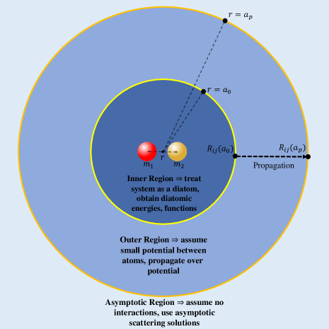
Figure 1: Schematic outlining the partitioning of space into an inner, outer and asymptotic region in the R-matrix method.

3 Analytic Scattering in Morse Oscillators

3.1 Morse Oscillator Solutions

When there is no angular momentum and hence no centrifugal term, the Morse potential for a diatom as a function of the internuclear distance $r$ has the algebraic form:

$$V(r)=D_{e}\left(\left(1-e^{-a_{\rm{Morse}}(r-r_{e})}\right)^{2}-1\right),$$ (8)

where $D_{e}$ is the well depth (assuming the zero of potential energy is placed at the dissociation energy), $r_{e}$ is the equilibrium position, or position of the well minimum, and $a_{\rm{Morse}}$ is a scaling parameter (the so-called Morse parameter) affecting the shape of the well.

The analytic eigenfunctions and eigenenergies of the Schrödinger equation with a Morse potential are well known. For the radial time-independent Schrödinger equation

$$\left(-\frac{\hbar^{2}}{2m}\frac{d^{2}}{dr^{2}}+D_{e}e^{-2a_{\rm{Morse}}(r-r_{e})}-2D_{e}e^{-a_{\rm{Morse}}(r-r_{e})}\right)\Psi_{n}=E_{n}\Psi_{n},$$ (9)

the bound eigenenergies $E_{n}$ and eigenfunctions $\Psi_{n}$ are given by [27]:

$$E_{n}^{\rm Morse}=-D_{e}+2a_{\rm{Morse}}\sqrt{\frac{D_{e}\hbar^{2}}{2\mu}}\left(n+\frac{1}{2}\right)-\frac{1}{4D_{e}}\left(2a_{\rm{Morse}}\sqrt{\frac{D_{e}\hbar^{2}}{2\mu}}\left(n+\frac{1}{2}\right)\right)^{2},$$ (10)

and

$$\Psi_{n}^{\rm Morse}=N_{n}z^{\left(1/(a_{\rm{Morse}}r_{0})-n-1/2\right)}\exp{\left(\frac{-z}{2}\right)}L_{n}^{\left(2/(a_{\rm{Morse}}r_{0})-2n-1\right)}(z),$$ (11)

where $L_{n}^{(\alpha)}(z)$ is the $n^{\rm th}$ associated Laguerre polynomial, and $N_{n}$ is a normalising factor given by

$$N_{n}=\left(\frac{\left(\frac{2}{a_{\rm{Morse}}r_{0}}-2n-1\right)a_{\rm{Morse}}\Gamma\left(n+1\right)}{\Gamma\left(\frac{2}{a_{\rm{Morse}}r_{0}}-n\right)}\right)^{\frac{1}{2}},$$ (12)

where $\Gamma(x)$ is the standard Gamma function.

3.2 Scattering Observables

It is possible to derive analytic scattering observables for a quantum scattering event involving the Morse oscillator potential energy curve because the time-independent Schrödinger equation with a Morse potential is analytically soluble.

Similar to Eq. (9), for a scattering event between particles with reduced mass $\mu$ with energy $E$ interacting over a Morse potential, the radial wavefunction $\Psi(r)$ is given by the time-independent radial Schrödinger equation:

$$\left(-\frac{\hbar^{2}}{2\mu}\frac{d^{2}}{dr^{2}}+D_{e}e^{-2a_{\rm{Morse}}(r-r_{e})}-2D_{e}e^{-a_{\rm{Morse}}(r-r_{e})}\right)\psi=E\psi.$$ (13)

By defining

$$k=\sqrt{\frac{2\mu E}{\hbar^{2}}},$$ (14)

one constraint that may be placed on $\psi(r)$ is that in the no-potential limit it must behave like the wavefunction of a free particle, i.e. it must be a plane wave. Likewise, this means that in the infinite distance limit where the potential’s strength tends to zero, the wavefunction must be sinusoidal such that:

$$\lim_{r\to\infty}\psi(r)=\sin(kr+\delta(k)),$$ (15)

where $\delta(k)$ is defined to be the phase shift (also known as the eigenphase) induced in the particle by its interaction with the potential.

Furthermore, by defining

$$r_{0}=\sqrt{\frac{\hbar^{2}}{2\mu D_{e}}},$$ (16)

$$z(r)=\frac{2}{a_{\rm{Morse}}r_{0}}e^{-a(r-r_{e})},$$ (17)

and

$$\Phi(z)=z^{\frac{1}{2}}\psi(z),$$ (18)

then it can be shown [28] that Eq. (13) can be re-written as

$$\frac{d^{2}\Phi}{dz^{2}}+\left(-\frac{1}{4}+\frac{1}{a_{\rm{Morse}}r_{0}z}+\frac{\frac{1}{4}+\left(\frac{k}{a_{\rm{Morse}}}\right)^{2}}{z^{2}}\right)\Phi(z)=0.$$ (19)

In this form, the equation is equivalent to the well-known Whittaker equation, whose solutions are the Whittaker functions. There are two linearly independent solutions to Eq. (19):

$$\psi_{\pm}(z)=e^{-z/2}z^{\pm ik/a_{\rm{Morse}}}{}_{1}F_{1}\left(\frac{1}{2}-\frac{1}{a_{\rm{Morse}}r_{0}}\pm\frac{ik}{a_{\rm{Morse}}},1\pm\frac{2ik}{a_{\rm{Morse}}};z\right),$$ (20)

where ${}_{1}F_{1}(x,y;z)$ is the Kummer confluent hypergeometric function of the first kind, and the $\psi_{\pm}(z)$ functions represent incoming and outgoing waves.

Using the results for the analytic scattering wavefunctions of the Morse potential in Eq. (20), it is possible to construct an analytic equation for the eigenphase $\delta(k)$ associated with scattering with the Morse potential. The eigenphase of the scattering event is desired because it can be used to generate other observables such as the cross section and scattering length.

The derivation below follows that of Rawitscher et al. [28] and Selg [29, 30].

The general solution $\psi(r)$ to Eq. (13) can be written in terms of the two solutions to Eq. (19), which are given by Eq. (20), such that:

$$\psi(r)=C_{+}\psi_{+}(r)+C_{-}\psi_{-}(r),$$ (21)

where $C_{\pm}$ are two constants.

There are two boundary conditions on $\psi(r)$ that can be used to obtain an expression for the eigenphase. Firstly, the asymptotic radial function must vanish at $r=0$, such that $\psi(0)=0$. This fact can be used to express one of the $C_{\pm}$ coefficients in terms of the other. Secondly the $r\to\infty$ asymptotic limit is given by Eq. (15). As $r\to\infty$, $z\to 0$. This means that due to a property of the Kummer confluent hypergeometric functions, both hypergeometric functions tend to $1$ as $r\to\infty$.

The S-matrix can be defined in the $r\to\infty$ limit as the negative of the ratio of the coefficients of the outgoing plane wave component of the asymptotic radial wavefunction to the incoming plane wave component [4].

Then, by defining $z_{0}$ such that

$$z(r=0)=z_{0}=\frac{2}{a_{\rm{Morse}}r_{0}}e^{ar_{e}},$$ (22)

the following expression can be obtained:

$$\left(\frac{z}{z_{0}}\right)^{\pm\frac{ik}{a_{\rm{Morse}}}}=e^{\mp ikr}.$$ (23)

Using the boundary conditions and Eq. (23), one can obtain an expression for the ratio of the coefficients of $\psi_{\pm}$ in this limit, and hence one can obtain an analytic expression for the S-matrix:

$$S(k)=\lim_{r\to\infty}\frac{C_{+}}{C_{-}}=\frac{{}_{1}F_{1}\left(\frac{1}{2}-\frac{1}{a_{\rm{Morse}}r_{0}}+\frac{ik}{a_{\rm{Morse}}},1+\frac{2ik}{a_{\rm{Morse}}};z_{0}\right)}{{}_{1}F_{1}\left(\frac{1}{2}-\frac{1}{a_{\rm{Morse}}r_{0}}-\frac{ik}{a_{\rm{Morse}}},1-\frac{2ik}{a_{\rm{Morse}}};z_{0}\right)}.$$ (24)

Besides Eq. (15), another way of defining the eigenphase is as the argument of the S-matrix, such that:

$$S(k)=e^{2i\delta(k)}.$$ (25)

Note that the factor of $2$ in the exponent is arbitrary, and other authors define it differently, depending on whether the eigenphase is defined as the argument of the S-matrix (as in [29]), or as the arctangent of the K-matrix, which is equivalent to defining the eigenphase to be half of the argument of the S-matrix (as in this work, and Ref. [28]).

The analytic expression for the eigenphase is then given by:

$$\delta(k)=\frac{1}{2}\arg\left(\frac{{}_{1}F_{1}\left(\frac{1}{2}-\frac{1}{a_{\rm{Morse}}r_{0}}+\frac{ik}{a_{\rm{Morse}}},1+\frac{2ik}{a_{\rm{Morse}}};z_{0}\right)}{{}_{1}F_{1}\left(\frac{1}{2}-\frac{1}{a_{\rm{Morse}}r_{0}}-\frac{ik}{a_{\rm{Morse}}},1-\frac{2ik}{a_{\rm{Morse}}};z_{0}\right)}\right).$$ (26)

Once the eigenphase has been obtained for a given Morse potential, then many scattering observables can be derived, including the K-matrix, and the T-matrix (also known as the transition matrix):

$$K(k)=\tan{\delta(k)},$$ (27)

$$S(k)=\frac{1-iK(k)}{1+iK(k)},$$ (28)

$$T(k)=S(k)-1.$$ (29)

Note that other authors use different definitions of the T-matrix such as the negative of its definition given here.

The total cross section at a given energy, $\sigma_{\rm tot}(k)$, which is the integral of the differential cross section over all solid angles, can be obtained from the eigenphase:

$$\sigma_{\rm tot}(k)=\frac{4\pi}{k^{2}}\sin^{2}(\delta(k)).$$ (30)

Finally the scattering length, $A$, and the effective range, $r_{\rm eff}$, are characteristic length scales associated with low-energy scattering. $A$ is defined as the limit

$$A=\lim_{k\to 0}\left(\frac{-\tan(\delta(k))}{k}\right),$$ (31)

for the $J=0$, s-wave (lowest energy) eigenphase [4]. The scattering length can be thought of as the low-energy $k\rightarrow 0$ limit of the gradient of the eigenphase. The effective range can be analytically determined through an integral over all space of the difference between the zero-energy scattering wavefunction, and the zero-energy potential-free scattering wavefunction [31]. It can be thought of as a length parameter which measures the overall effect the potential has on the scattering event, since it is defined by the difference between scattering in the cases with and without a potential. As such, calling it the effective range of the potential is natural.

One way of obtaining these two quantities from the eigenphase is by taking a Taylor expansion of the eigenphase close to zero scattering energy [4]:

$$k\cot{\delta(k)}=\frac{-1}{A}+\frac{1}{2}r_{\rm{eff}}k^{2}+O(k^{4}).$$ (32)

4 Method

4.1 Potentials Investigated

The main Morse potential used in this work is presented in Fig. (2). This Morse potential uses parameters with reduced mass of $\mu=33.71525621$ Da (and a value of $\hbar$ obtained from Qiang and Dong [32]). The value for $\mu$ was chosen for numerical convenience when testing the algorithm, as it meant that $\hbar^{2}/2\mu$ had a value of $0.5$ to seven decimal places in the units of $\rm{cm}^{-1}$ and Å used in this work. The specific value used for $a_{\rm{Morse}}$ was chosen such that the ground state eigenenergy was 90 $\rm{cm}^{-1}$ to six decimal places, for ease of comparison. The values of $D_{e}$ and $r_{e}$ used in this work were chosen in analogy with the $\rm{Ar}_{2}$ dimer, which is currently being used to investigate the application of this method to more sophisticated potentials. The analytic eigenenergies were generated from these parameters and Eq. (10).

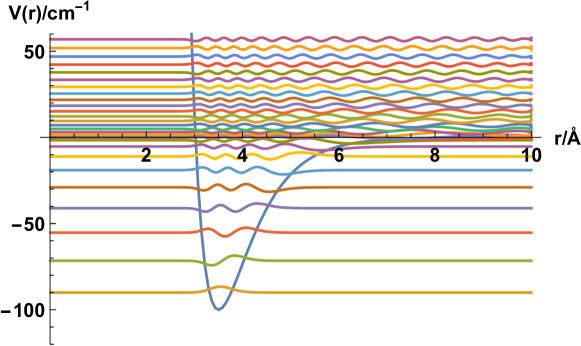
Figure 2: A Morse oscillator potential energy curve for an $\rm{Ar}_{2}$-like potential with $D_{e}=100$ $\rm{cm}^{-1}$, $r_{e}=3.5$ Å, $a_{\rm{Morse}}=1.451455517$ Å^-1. Wavefunctions of the vibrational bound states are also shown at their associated eigenenergies, along with with the continuum states between $0$ and $60$ $\rm{cm}^{-1}$ . The bound and continuum states were generated by solving the Schrödinger equation with $\mu=33.71525621$ Da with an R-matrix method with a boundary of $10$ Å.

Other Morse potentials were tested, notably several obtained from [33] for actual diatoms: LiH, $\rm{H}_{2}$, HCl, and CO. Fig. (3) shows one of these potentials: LiH. In this paper, we present only results for the Morse potential shown in Fig. (2). Similar numerical behaviour was observed for all of the potentials tested, however.

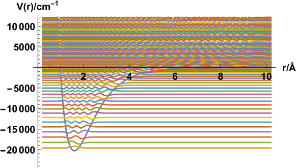
Figure 3: Morse oscillator potential and states for LiH. Parameters used are $D_{e}=20287.62581$ $\rm{cm}^{-1}$, $r_{e}=1.5956$ Å, $a_{\rm{Morse}}=1.128$ Å^-1 [33]. The states were generated by solving the Schrödinger equation with $\mu=0.8801221$ Da [33] with an R-matrix method with a boundary of $10$ Å.

4.2 Numerical Details

The R-matrix method was used to generate scattering results, including the eigenphase and the scattering length, for the single-channel, $J=0$ Morse oscillator potential. These results are compared with the analytic results quoted above.

In the construction of the R-matrix, the inner region bound system was solved numerically to generate the bound eigenenergies and radial eigenfunctions of two particles interacting over a Morse potential well. To generate the numeric results, $N=200$ grid points and eigenfunctions were used to obtain the inner region eigenenergies (and amplitudes) using the Lobatto shape functions DVR method outlined in section 2. The inner region was defined to range from $r_{\rm{min}}=0.01$Å to $a_{0}=10.0$Å.

The R-matrix was then constructed on the boundary and propagated to an asymptotic radius. For the results presented in the following, the propagation was performed from $a_{0}=10.0$ Å to $a_{p}=25.0$ Å, with $N_{\rm{prop}}=2500$ iterations of the propagation equation over a uniform grid. The propagated R-matrix was then used to construct the eigenphase for the $J=0$ Morse scattering event.

To explore the low-energy behaviour of the numeric method, the analytic and numeric eigenphases were used to generate the scattering length and effective range. This was done by fitting the low-energy plot to the form given in Eq. (32) using Mathematica’s FindFit function over the lower scattering energy range $k=0.0004$ Å to $k=0.001$ Å. (This is equivalent to $E=8.0\times 10^{-8}$ $\rm{cm}^{-1}$ to $E=5.0\times 10^{-7}$ $\rm{cm}^{-1}$ for this system.)

5 Results

5.1 Comparison between analytic and numerical RmatReact results

Figure 4: The same Morse oscillator potential as in Fig. (2). Energy levels of the continuum states generated by the R-matrix below below $60$ $\rm{cm}^{-1}$ are coloured differently to the vibrational bound states in order to distinguish the states close to dissociation from the states just above dissociation. The R-matrix inner region boundary, $a_{0}=10$ Å, is also highlighted.

The numerical and analytic results for the eigenenergies are presented in Table 1. For low-lying states whose wavefunctions are essentially completely contained in the inner region, the agreement between the two methods is excellent. The final two states are more diffuse, as seen in Fig. (2), and hence they are more likely to have significant amplitude outside the inner region. Due to this, the inner region solution energies lies slightly below the true answer.

Table 1: Comparison of the analytic and numeric bound eigenenergies of the Morse diatomic system for vibrational energy levels $n=0$ to $9$. The relative error refers to the difference between each level’s numeric and analytic values, divided by the analytic value (analytic minus numeric, divided by analytic).

$n$	Analytic / $\rm{cm}^{-1}$	R-matrix / $\rm{cm}^{-1}$	Relative error
$0$	$-90.000000$	$-90.000000$	$1.73\times 10^{-12}$
$1$	$-71.580042$	$-71.580042$	$4.59\times 10^{-11}$
$2$	$-55.266807$	$-55.266807$	$1.30\times 10^{-11}$
$3$	$-41.060295$	$-41.060295$	$1.82\times 10^{-11}$
$4$	$-28.960506$	$-28.960506$	$5.73\times 10^{-12}$
$5$	$-18.967441$	$-18.967441$	$1.33\times 10^{-12}$
$6$	$-11.081099$	$-11.081099$	$3.25\times 10^{-12}$
$7$	$-5.3014807$	$-5.3014807$	$-6.42\times 10^{-12}$
$8$	$-1.6285853$	$-1.6286033$	$-0.000011$
$9$	$-0.062413189$	$-0.094633937$	$-0.516$

Figure 5 compares the RmatReact numerical eigenphase to the analytic solution for the eigenphase given by Eq. (26) over the scattering energy range of $0.001$ to $0.1$ $\rm{cm}^{-1}$ ($0.00144$ to $0.144$ K). The root mean square difference between the analytic and numeric results is approximately $4.6\times 10^{-5}$ radians, which is small.

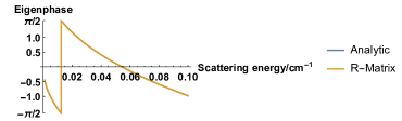
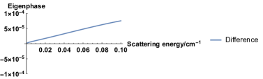
Figure 5: Upper plot: eigenphase (in radians) for a scattering event for the Morse potential of Fig. 2 calculated both analytically and using R-matrix methodology. The two lines overlap. Lower plot: difference (analytic $-$ R-matrix) in eigenphase (in radians) between the two methods.

Analytic and numerical results for scattering length and effective range are presented in Table 2. Again the results given by the two methods are very similar.

Table 2: Table of comparisons for the analytic and numeric scattering length and effective range. The relative error refers to the difference between each quantity’s numeric and analytic values divided by the analytic value (analytic minus numeric, divided by analytic).

	Analytic/Å	R-matrix/Å	Relative error
Scattering Length	$10.166078$	$10.166133$	$-5.34\times 10^{-6}$
Effective Range	$1.6537298$	$1.6667562$	$-0.00788$

5.2 Numerical Parameters

To investigate the accuracy of the R-matrix method in comparison to the analytic results, the numerical parameters used in the algorithm were varied and the resultant error was plotted. The seven numerical parameters which the method relies on are summarised in Table 3.

To encapsulate all of the information in the lower plot of Fig. (5) in one number, the error metric used was the root mean square deviation (RMSD) between the eigenphase, $\delta(E)$ calculated using the R-matrix method ($\delta_{\rm{num}}(E)$) and the analytic eigenphase ($\delta_{\rm{ana}}(E)$). The eigenphase was calculated for $100$ equally spaced scattering energy values between $0.001$ and $0.1$ $\rm{cm}^{-1}$. The error characteristic, the RMSD, was then calculated using:

$$\delta_{\rm{RMSD}}=\sum_{i=1}^{100}\sqrt{\frac{(\delta_{\rm{ana}}(E_{i})-\delta_{\rm{num}}(E_{i}))^{2}}{100}}.$$ (33)

A version of this error metric which involved (numerically) integrating the squared difference over the energy range was tested, and found to give the same results as merely sampling over $100$ equally spaced points in the energy range. Plotting $\delta_{\rm{RMSD}}$ as a function of different error parameters facilitated the assessment of the numerical stability of the method. These plots can be found in Fig. (6). For all of the plots in Fig. (6), $r_{\rm{min}}$ was kept constant at $0.01$Å.

Table 3: Table of numerical parameters

Symbol	Definition	Units
$N$	Number of inner region states and grid points	Unitless
$N_{\rm{prop}}$	Number of propagation points	Unitless
$r_{\rm{min}}$	Start of inner region	$\rm{\AA}$
$a_{0}$	End of inner region and start of propagation	$\rm{\AA}$
$a_{p}$	End of propagation	$\rm{\AA}$
$\Delta r$	$\frac{a_{0}-r_{\rm{min}}}{N-1}$ Average inner region grid spacing	$\rm{\AA}$
$\Delta r_{\rm{prop}}$	$\frac{a_{p}-a_{0}}{N-1}$ Average propagator grid spacing	$\rm{\AA}$

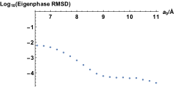
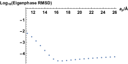
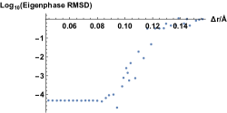
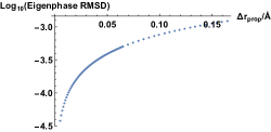
Figure 6: Top left: The log of the RMSD of the eigenphase plotted against $a_{0}$ between $6.5$Å and $11$Å. The other parameters were held constant at $N=200$, $N_{\rm{prop}}=2500$, $r_{\rm{prop}}=25$Å.
Top right: The log of the RMSD of the eigenphase plotted against $a_{p}$ between $11$Å and $26$Å. The other parameters were held constant at $N=200$, $N_{\rm{prop}}=2500$, $a_{0}=10$Å.
Middle left: The log of the RMSD of the eigenphase plotted against $N$ between $20$ and $220$. The other parameters were held constant at $N_{\rm{prop}}=2500$, $a_{0}=10$Å, $r_{\rm{prop}}=25$Å.
Middle right: The log of the RMSD of the eigenphase plotted against $N_{\rm{prop}}$ between $500$ and $2500$. The other parameters were held constant at $N=200$, $a_{0}=10$Å, $r_{\rm{prop}}=25$Å.
Bottom left: The log of the RMSD of the eigenphase plotted against $\Delta r$ between $0.0445982$Å and $0.156094$Å. $N$ was allowed to vary between $223$ and $63$ to vary $\Delta r$. The other parameters were held constant at $a_{0}=10$Å, $N_{\rm{prop}}=2500$, $r_{\rm{prop}}=25$.
Bottom right: The log of the RMSD of the eigenphase plotted against $\Delta r_{\rm{prop}}$ between $0.005$Å and $0.164835$Å. $N_{\rm{prop}}$ was allowed to vary between $3000$ and $90$ to vary $\Delta r_{\rm{prop}}$. The other parameters were held constant at $N=200$, $a_{0}=10$Å, $r_{\rm{prop}}=25$.

When varying $a_{0}$, any $a_{0}$ value above approximately $9$ Å appears to produce converged results where the error changes very little. This is likely because a value of $a_{0}$ which is too small cannot accurately ‘capture’ all of the bound states of the potential well. Since the final bound state is of the order $10^{-2}$ $\rm{cm}^{-1}$ in depth, $V(a_{0})$ must be approximately of that order for the state to be found by the method.

When varying $a_{p}$, any value above $16$ Å appears to produce converged results; however, the error increases slightly as $a_{p}$ is extended beyond $16$ Å. This is likely due to $\Delta r_{\rm{prop}}$ increasing as $N_{\rm{prop}}$ is held constant, which decreases the accuracy of the approximations made in the propagator method.

When varying $N$ and $\Delta r$ (where $\Delta r$ is increased by decreasing $N$ and vice-versa), there is a clear point where increasing $N$ further has no effect, but where decreasing $N$ even slightly significantly increases the error. This suggests that the method is converging on a solution once the grid spacing is sufficiently small, as is common in numerical integration techniques. This further suggests that this solution’s RMSD from the analytic solution is approximately $10^{-4}$.

Finally, when varying $N_{\rm{prop}}$ and $\Delta r_{\rm{prop}}$, the method appears to produce results with very low error for all values of $N_{\rm{prop}}$ and $\Delta r_{\rm{prop}}$ tested, with only slight variation in the error recorded. This suggests that it is possible to propagate the R-matrix using very few, very wide steps and still produce accurate results. However, this may be a consequence of using as the test potential the Morse oscillator potential, since it decreases exponentially with distance and thus varies very little in the outer region. More relatistic potentials are longer-range and multipolar in nature at large $r$, so narrower steps may be needed in the propagation.

6 Conclusions and outlook

We clearly demonstrate that we can obtain excellent results using our R-matrix implementation for low-energy scattering within a Morse oscillator potential. Asymptotically this potential decays exponentially, which makes it unlike physical potentials, which have a much longer range. Physical potentials decay as $r^{-n}$, where $n$ is a positive integer.

The next step is to implement DVR shape functions into variational nuclear motion codes to facilitate the calculation of boundary amplitudes within these codes. This been done for the general diatomic code Duo [16] and triatomic code DVR3D [17]. The diatomic problems for which tests have been run so far all involve a single asymptotic channel, which makes R-matrix propagation straightforward. In general this will not be true and it will be necessary to consider multichannel problems. To address this issue we have successfully performed propagations with a general code originally designed for electron – atom problems [34]. This code now needs generalising to provide automated resonance fitting [35, 36] and bound state finding [37] features.

We intend to use this new methodology on physical problems, and to create a generalisation of the R-matrix formalism to allow the explicit treatment of reactive processes. We have conducted preliminary tests similar to the ones presented here on more accurate Ar – Ar potentials with multipolar long-range expansions, for which the leading term is $n=6$, and also obtained excellent results. All of these results will be reported elsewhere.

References

- [1] B.K. Stuhl, M.T. Hummon, J. Ye, Annu. Rev. Phys. Chem. 65, 501 (2014). 10.1146/annurev-physchem-040513-103744
- [2] G. Quemener, P.S. Julienne, Chem. Rev. 112, 4949 (2012)
- [3] J. Tennyson, L.K. McKemmish, T. Rivlin, Faraday Discuss. 195, 31 (2016). 10.1039/c6fd00110f
- [4] P.G. Burke, R-Matrix Theory of Atomic Collisions: Application to Atomic, Molecular and Optical Processes, vol. 61 (Springer Science & Business Media, 2011)
- [5] J. Tennyson, Phys. Rep. 491, 29 (2010)
- [6] P. Descouvemont, D. Baye, Reports on progress in physics 73, 036301 (2010)
- [7] J. Tennyson, Chem. Phys. Lett. 86, 181 (1982)
- [8] O.L. Polyansky, A. Alijah, N.F. Zobov, I.I. Mizus, R. Ovsyannikov, J. Tennyson, T. Szidarovszky, A.G. Császár, Phil. Trans. Royal Soc. London A 370, 5014 (2012)
- [9] A. Carrington, I.R. McNab, Acc. Chem. Res. 22, 218 (1989). 10.1021/ar00162a004
- [10] M. Mayle, G. Quemener, B.P. Ruzic, J.L. Bohn, Phys. Rev. A 87, 012709 (2013). 10.1103/PhysRevA.87.012709
- [11] N.F. Zobov, S.V. Shirin, L. Lodi, B.C. Silva, J. Tennyson, A.G. Császár, O.L. Polyansky, Chem. Phys. Lett. 507, 48 (2011)
- [12] T. Szidarovszky, A.G. Csaszar, Mol. Phys. 111, 2131 (2013). 10.1080/00268976.2013.793831
- [13] B.C. Silva, P. Barletta, J.J. Munro, J. Tennyson, J. Chem. Phys. 128, 244312 (2008)
- [14] M. Pavanello, L. Adamowicz, A. Alijah, N.F. Zobov, I.I. Mizus, O.L. Polyansky, J. Tennyson, T. Szidarovszky, A.G. Császár, M. Berg, A. Petrignani, A. Wolf, Phys. Rev. Lett. 108, 023002 (2012)
- [15] M. Lara, P.G. Jambrina, F.J. Aoiz, J.M. Launay, J. Chem. Phys. 143, 204305 (2015). 10.1063/1.4936144
- [16] S.N. Yurchenko, L. Lodi, J. Tennyson, A.V. Stolyarov, Comput. Phys. Commun. 202, 262 (2016). 10.1016/j.cpc.2015.12.021
- [17] J. Tennyson, M.A. Kostin, P. Barletta, G.J. Harris, O.L. Polyansky, J. Ramanlal, N.F. Zobov, Comput. Phys. Commun. 163, 85 (2004)
- [18] I.N. Kozin, M.M. Law, J. Tennyson, J.M. Hutson, Comput. Phys. Commun. 163, 117 (2004)
- [19] S. Yurchenko, P. Jensen, W. Thiel, J. Chem. Phys. 71, 281 (2004)
- [20] S. Yurchenko, P. Jensen, W. Thiel, J. Chem. Phys. 90, 333 (2010)
- [21] H.Y. Mussa, J. Tennyson, Comput. Phys. Commun. 128, 434 (2000)
- [22] J.C. Light, T. Carrington, Adv. Chem. Phys. 114, 263 (2000). 10.1002/9780470141731.ch4
- [23] D. Manolopoulos, in Numerical Grid Methods and Their Application to Schrödinger’s Equation (Springer, 1993), pp. 57–68
- [24] D. Manolopoulos, R. Wyatt, Chem. Phys. Lett. 152, 23 (1988)
- [25] E.W. Weisstein. Lobatto quadrature From MathWorld—A Wolfram Web Resource. URL “url–http://mathworld.wolfram.com/LobattoQuadrature.html˝. Last visited on 22/11/16
- [26] R.B. Walker, J.C. Light, Ann. Rev. Phys. Chem. 31, 401 (1980). 10.1146/annurev.pc.31.100180.002153
- [27] P.M. Morse, Phys. Rev. 34, 57 (1929)
- [28] G. Rawitscher, C. Merow, M. Nguyen, I. Simbotin, Am. J. Phys. 70, 935 (2002)
- [29] M. Selg, Proceedings of the Estonian Academy of Sciences 65, 267 (2016)
- [30] M. Selg, J. Chem. Phys. 136, 114113 (2012)
- [31] H. Bethe, Phys. Rev. 76, 38 (1949)
- [32] P.J. Mohr, B.N. Taylor, D.B. Newell, J. Phys. Chem. Ref. Data 84, 1527 (2012)
- [33] W.C. Qiang, S.H. Dong, Phys. Letts. A 363, 169 (2007)
- [34] V.M. Burke, C.J. Noble, Computer Phys. Comm. 85, 471 (1995)
- [35] J. Tennyson, C.J. Noble, Comput. Phys. Commun. 33, 421 (1984)
- [36] D.A. Little, J. Tennyson, M. Plummer, A. Sunderland, Comput. Phys. Commun. 215, 137 (2017). 10.1016/j.cpc.2017.01.005
- [37] B.K. Sarpal, S.E. Branchett, J. Tennyson, L.A. Morgan, J. Phys. B: At. Mol. Opt. Phys. 24, 3685 (1991)