Crossover between tricritical and Lifshitz points in pyrochlore FeF₃

Abstract

Pyrochlore FeF₃ (pyr-FeF₃) is a Heisenberg anti-ferromagnetic (AF) with a magnetic susceptibility deviating from the Curie-Weiss law, even at the room temperature. This compound shows a transition to a long-range ordered state with all-in all-out (AIAO) spin configuration. The critical properties of this transition have remained a matter of dispute. In this work, to gain more insight into the critical properties of pyr-FeF₃, using ab initio density functional theory (DFT), we obtain spin Hamiltonian of this material under the relative volume change with respect to the experimental volume ($\frac{\Delta V}{V_{0}}$) from $-0.2$ to $0.2$. We show that the relevant terms in the spin Hamiltonians are the AF exchange up to third neighbors, the nearest neighbor bi-quadratic and the direct Dyzaloshinski-Moriya (DM) interactions and find how these coupling constants vary under the volume change. Then we study the effect of volume change on the finite temperature critical behavior, using classical Monte Carlo (MC) simulation. We show that the spin system undergoes a weakly first order transition to AIAO at small volumes which turns to a second order transition close to the experimental structure. However, increasing $\frac{\Delta V}{V_{0}}$ to $\sim 0.2$, systems shows a transition to a modular spin structure. This finding suggests the existence of a Lifshitz point in pyr-FeF₃ and may explain the unusual critical exponents observed for this compound.

I introduction

During the past few years, curious behavior of geometric frustrated pyrochlores have been a topic of constant significance due to their interesting peculiar physics Zhou et al. (2017); Petit et al. (2016); Ramirez (1994); Henelius et al. (2016); Fåk et al. (2012); Gardner et al. (2010); Sohn et al. (2017); Zhang et al. (2017); Ueda et al. (2012); Sadeghi et al. (2015); Lacroix et al. (2011). Geometrically frustrated pyrochlore is a three-dimensional lattice consisting of corner-sharing tetrahedra in which the magnetic ions are placed on the corner of each tetrahedron, mostly with anti-ferromagnetic interaction between nearest neighbors. In these systems, magnetic properties deviate from conventional magnetic systems, in a sense that magnetic moments do not tend to form a long range ordering even at the temperatures much below the Curie-Weiss temperature ($\Theta_{\mathrm{CW}}$). The reason for such a strange behavior is in the geometry of the system where the local energy optimization does not tend to a unique global minimum, which gives rise to an extensive ground state degeneracy. As a result, geometrically frustrated materials have been found to exhibit a wealth of exotic ground states and behaviors such as spin glassSingh and Lee (2012), spin ice Bramwell and Gingras (2001) or even spin liquidSavary and Balents (2017). pyr-FeF₃ is an anti-ferromagnet Heisenberg pyrochlore which shows a transition to a long range ordered state at a temperature much smaller than its Curie-Weiss temperature and its susceptibility also deviates from the Curie-Weiss law even at room temperature Ferey et al. (1986). The structure of pyr-FeF₃ is faced-center cubic with space group Fd3̄m, where Fe atoms occupy the 16c (0,0,0) sites and fluorine the 48f (x, 1/8, 1/8) sites Pape and Ferey (1986). Indeed, the Fe atoms reside on the corners of each tetrahedron while each fluorine lays in a position between any two irons but not exactly on the edge, henceforth giving rise to a 142.3^∘ Fe-F-Fe bond angle. The experimental values for the lattice parameter and internal parameter (x) (which determines the Fe-F-Fe bond angle) are 19.511 (a.u.) and 0.3104(5), respectivelyPape and Ferey (1986). Experimental resultsCalage et al. (1987) (Mössbauer experiments) show that the transition temperature is about 20 K where, below this temperature, the Fe magnetic moments point toward or out of the tetrahedron centers, that is the so called all-in/all-out (AIAO) ordering. Another interesting peculiarity of pyr-FeF₃ is the universality class of its transition to ALAO, measured by the order parameter exponent $\beta\sim 0.18\pm 0.02$ Reimers et al. (1992) which deviates from the known universalities such as Ising ($\beta\approx 1/3$), Heisenberg ($\beta\approx 1/3$) or the tricritical point ($\beta=1/4$). In Ref. [Sadeghi et al., 2015], using ab initio method based on density functional theory (DFT), we proposed a spin Hamiltonian for pyr-FeF₃ in its experimental structure. The dominant terms in the spin Hamiltonian were found to be the nearest neighbor AF Heisenberg, positive bi-quadratic and direct Dyzaloshinskii-Moriya (DM) interactions. The classical Monte Carlo (MC) simulation of this Hamiltonian reveals a transition to the ALAO state at the critical temperature $T_{C}=20$K and the value of the order parameter critical exponent was evaluated as $\beta=0.18\pm 0.02$ in agreement with the neutron scattering experimentsReimers et al. (1990). It has also been shown that the systems enters in a Coulomb phase state for a wide temperature range from $20$K to $\sim 100$K. The anomalous critical exponent observed for pyr-FeF₃, suggests that this compound in its experimental structure might be located near a multi-critical point. If so, a relatively little change in the parameters of the Hamiltonian may change the critical behavior of the system. Since, the magnetic exchange couplings are highly sensitive to the magnetic ion distances and the bond angles, the variation of the spin Hamiltonian parameters can be calculated as a function of volume change in a way that all the symmetries of the lattice are preserved. Based on this motivation, we aim to shed light on the critical properties of pyr-FeF₃ by obtaining its spin Hamiltonian in the presence of hydrostatic positive (negative) pressure through decreasing (increasing) its volume at the ambient pressure. Experimentally, the change in the volume can also be done through chemical pressure which means the substitution of some elements in a given compound by smaller (positive pressure) or larger (negative pressure) elements  Hallas et al. (2014). Once the spin Hamiltonian is found, for each volume change the finite temperature critical behavior of the system can be investigated by the classical MC simulation.

The paper is organized as the following. Section II gives the details of DFT method and MC simulation. In section III, the structural variations under pressure, the resulting spin Hamiltonian for each volume change and the corresponding critical properties at finite temperature are discussed and finally, the end of this paper is devoted to the conclusion.

II Computational methods

In this paper, we employ Density Functional Theory (DFT) to construct an effective spin model Hamiltonian ($H_{spin}$) for pyr-FeF₃. The methods of calculation for different terms of spin Hamiltonian have been reported in Ref.[Sadeghi et al., 2015]. To this end, We use the FLEUR FLEURgroup (full-potential augmented plane wave (FLAPW) basis sets code). The exchange and correlation effects are considered using Perdew Burke Ernzerhof (PBE) functional from generalized gradient approximation (GGA) Perdew et al. (1996). To improve electron-electron repulsion, we employ Hubbard correction within GGA+$U$ approximation. For the anisotropic spin Hamiltonian term (the Dzyaloshinskii-Moriya (DM) and the single-ion interactions Sadeghi et al. (2015)), spin-orbit coupling effects are considered (GGA+$U$+SOC). Brillouin zone integrations are performed using $4\times 4\times 4$ k-points sampling for the conventional unit-cell (64 atoms) to calculate the Heisenberg exchange coupling constants and $6\times 6\times 6$ k-points sampling for primitive cell (16 atoms) for calculating the DM, single-ion and bi-quadratic couplings. We use 2.0 and 1.35 (a.u.) for the Muffin-tin radius of Fe and F atoms, respectively and optimized $k_{\mathrm{max}}=4.2\,(\mathrm{a.u.})^{-1}$ for cutoff energy. Monte Carlo simulations are performed to find the critical properties of $H_{spin}$, using the replica exchange methodHukushima and Nemoto (1996). We use three-dimensional lattices consisting of $N\times L^{3}$ spins, where $L$ is the linear size of the simulation cell, which in this work we take $L=4,5,6,7,8,9,10,11$. For thermal equilibrium, we use $10^{6}$ Monte Carlo steps (MCS) per spin in each temperature and $10^{6}$ MCS for data collection. To reduce the correlation between the successive data, measurements are done after skipping 10 MCS.

III Results and Discussion

III.1 Structural geometry under pressure

It is known that in GGA+$U$ calculations, $U$ plays an important role, especially in magnetic properties. we use $U=3$eV and the Hund coupling $J_{H}=1$eV. We show that choosing these values for the on-site Coulomb repulsion give rise to reasonable results for the magnetic properties of pyr-FeF₃ in its experimental structure at the ambient pressure.

In this section, we consider the effect of volume change on the structural geometry in GGA+$U$ calculation. At each volume, we optimized the internal parameter ($x$) to find the minimum total energy of the system. The results show that as the volume decreases the optimized $x$ also increases, meaning that the Fe atoms in the lattice get closer to each other i.e. Fe-F-Fe bond angle and Fe-F bond distance become smaller. Fig. 1 shows the variations of the bond angle (Fe-F-Fe) and the bond distance (Fe-F) with respect to the fractional volume change. According to the Kanamori-Goodenough rule Kanamori (1959); Goodenough (1955), the larger bond angle (120-180) can lead to the anti-ferromagnetic exchange interaction between nearest neighbors, however, different bond distance has a more crucial effect on the strength of exchange interaction. So, at smaller lattice volumes, we expect to have stronger exchange interaction due to the shorter inter-ionic distance (see Fig. 1).

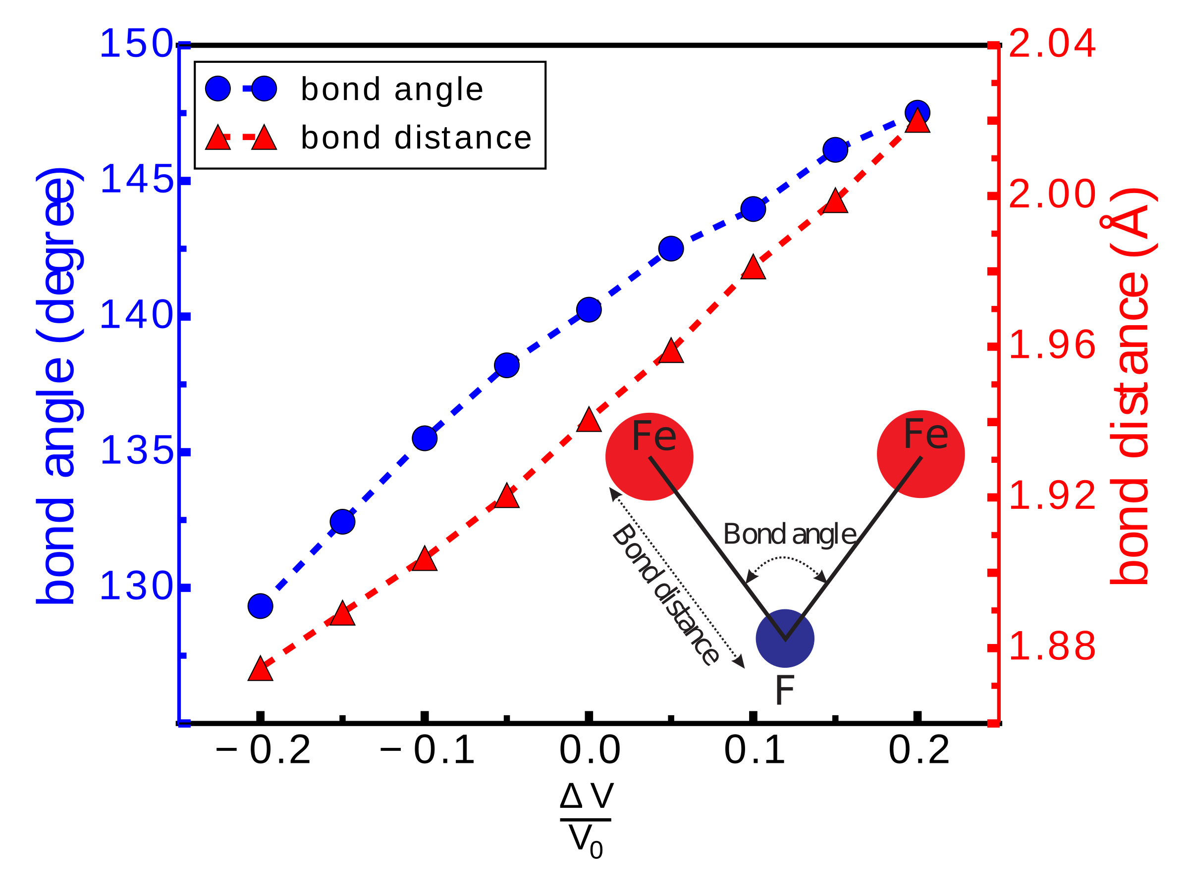
Figure 1: (Color online) The GGA+$U$ result for the variations of the Fe-F-Fe bond angle and Fe-F bond distance in pyr-FeF₃ versus the fractional volume change $\frac{\Delta V}{V_{0}}$. $V_{0}$ denotes the unit cell volume of the experimental structure.

III.2 Spin Hamiltonian

Now we proceed to derive an effective Hamiltonian to find the ground state and also the finite temperature properties of pyr-FeF₃. We define a model spin Hamiltonian that contains several spin-spin interactions, like Heisenberg, bi-quadratic, single-ion and direct Dzyaloshinskii-Moriya (DM) interactions:

$$\begin{split}H_{\rm{spin}}=\sum_{i\neq j}J_{ij}(\vec{S_{i}}\cdot\vec{S_{j}})+B\sum_{\rm n.n}(\vec{S_{i}}\cdot\vec{S_{j}})^{2}\\ +D\sum_{\rm n.n}\hat{D}_{ij}\cdot(\vec{S_{i}}\times\vec{S_{j}})+\Delta\sum_{i}(\vec{S_{i}}\cdot\vec{d_{i}})^{2}\end{split}$$ (1)

where $\vec{S_{i}}$ denotes a unit vector, $(J_{1},J_{2},J_{3a},J_{3b})$ are the Heisenberg couplings constants up to third neighbors (we assume $J_{3b}=0$, see Fig. 2), $B$ is the bi-quadratic coupling constant between the nearest neighbors, $D$ and $\Delta$ denote the strengths of DM and single-ion anisotropy, respectively. The unit vectors $\hat{D}_{ij}$ denote the directions of the direct DM vectors in pyrochlore Elhajal et al. (2005) . We estimate the Heisenberg coupling constants by mapping the collinear spin-polarized DFT total energies to the spin Hamiltonian (1), while for the bi-quadratic, DM and single-ion parameters we used the total energies obtained by the non-collinear spin-polarized DFT.

Figure 2: (Color online) pyr-FeF₃ structure with its corner-shared tetrahedrons in the cubic unit cell. Orange and gray spheres are $Fe^{3+}$ and $F^{-}$ ions, respectively. Different neighbors for Heisenberg interactions ($J_{1},J_{2},J_{3a},J_{3b}$) have been shown.

Fig. 3 shows the variations of $J_{1},J_{2}$ and $J_{3a}$ with respect to the fractional relative changes in the unit cell volume $\frac{\Delta V}{V_{0}}$, where $V_{0}$ denotes the unit cell volume of the experimental structure. This figure shows that the first and second neighbor Heisenberg coupling constants $J_{1}$ and $J_{2}$ rapidly decreases by increasing the volume, while the variation of $J_{3a}$ versus $\frac{\Delta V}{V_{0}}$ is much slower.

Figure 3: (Color online) Heisenberg coupling constants $J_{1},J_{2}$ and $J_{3a}$ versus the fractional change in the unit cell volume, $\frac{\Delta V}{V_{0}}$. $V_{0}$ denotes the unit cell volume of the experimental structure.

Figure 4: (Color online) Variation of nearest neighbor bi-quadratic coupling $B$ and the DM coupling versus the fractional change in the unit cell volume, $\frac{\Delta V}{V_{0}}$. $V_{0}$ denotes the unit cell volume of the experimental structure.

Figure 5: (Color online) AIAO order parameter versus temperature for $\frac{\Delta V}{V_{0}}=-0.2,0.0,0.15$. The data are obtained by the MC simulations on the lattices with $L=10$.

Fig. 4 illustrates the dependence of the $B$ and $D$ coupling constants on the fractional volumes changes, showing also the rapid fall of both interactions by increasing the unit cell volume. Interestingly, these results show the sign change of the bi-quadratic coupling from positive to negative at $\frac{\Delta V}{V_{0}}\sim 0.15$. Our calculations for the strength of single ion anisotropy ($\Delta$) results that in all the unit cell volumes its value is an order of magnitude less than $B$ and $D$, so we can neglect this term.

III.3 Monte Carlo simulations

In this section, we represent the MC results of the spin Hamiltonian (1) with the coupling constants obtained for the fractional volume changes $\frac{\Delta V}{V_{0}}=-0.2,-0.15,-0.1,-0.05,0.0,0.05,0.1,0.15,0.2$. We observe a phase transition to the all-in all-out (AIAO) long range order for $-0.2\leq\frac{\Delta V}{V_{0}}\leq 0.15$. This can be seen in Fig. 5, where the temperature behavior of the AIAO order parameter define by $m_{n}=(\sum^{4}_{i=1}S^{i}\cdot d^{i})/N$ ( with $d^{i}$ being denoted the four local cubic [111] directions and $N=4L^{3}$ the total number of spins) is plotted for $\frac{\Delta V}{V_{0}}=-0.2,0.0,0.15$ in the lattices with the linear size $L=10$. The AIAO ordering vanishes for $\frac{\Delta V}{V_{0}}=0.2$, however, we find a phase transition for this case and we will later discuss on its detail. The transition temperature $T_{C}$ decreases by increasing the volume from $\sim 50$K for $\frac{\Delta V}{V_{0}}=-0.2$ to $\sim 4$K for $\frac{\Delta V}{V_{0}}=0.2$ (see Tab.LABEL:tab1). The values of $T_{C}$ are estimated from location of the peaks in the specific heat exhibited in Fig.6. The last column in Table. LABEL:tab1 shows the values of Curie-Weiss temperature ($\Theta_{{\rm CW}}$) estimated by the linear extrapolation of the inverse susceptibility in the temperature interval $300$K to $400$K (Fig.7). Interestingly, the dependence of transition temperature to the ratio of the DM coupling to $J_{1}$ $(D/J_{1})$ is found to be linear as shown in Fig. 8.

Table 1: Critical and Curie-Weiss temperatures for different fractional volume changes.

$\frac{\Delta V}{V_{0}}$	$T_{C}({\rm K})$	$\Theta_{CW}({\rm K})$
0.20	$\sim 4$	$-725$
0.15	$\sim 7$	$-814$
0.10	$\sim 11$	$-881$
0.05	$\sim 16$	$-912$
0.00	$\sim 21$	$-973$
-0.05	$\sim 26$	$-1082$
-0.10	$\sim 33$	$-1136$
-0.15	$\sim 41$	$-1194$
-0.20	$\sim 50$	$-1221$

Figure 6: (Color online) Specific heat versus temperature for $\frac{\Delta V}{V_{0}}=-0.2,0.0,0.2$. The data are obtained by the MC simulations on the lattices with $L=10$.

Figure 7: (Color online) Temperature dependence of the inverse susceptibility for $\frac{\Delta V}{V_{0}}=-0.2,0.0,0.2$. The data are obtained by the MC simulations on the lattices with $L=10$. The dashed lines represent the linear fits to the inverse susceptibility in the temperature range $300$K to $400$K, where the Curie law holds. The Curie-Weiss temperatures are obtained by the intersection of the dashed lines and the T axis.

Figure 8: (Color online) Transition temperature $T_{C}$ versus $D/J_{1}$.

Figure 9: (Color online) The scaling behavior of the minimum of Binder forth energy cumulant $U_{{\rm min}}$ versus $L^{-3}$ for $\frac{\Delta V}{V_{0}}=-0.05,0.0,0.05$. The dashed lines are obtained by fitting Eq.3 to the data.

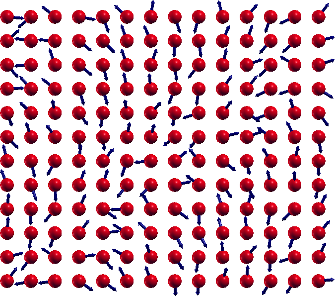
Figure 10: (Color online) A two dimensional of spin snapshot for $\frac{\Delta V}{V_{0}}=0.2$ obtained by MC simulation at $T=0.5$K for a lattice of linear size $L=10$.

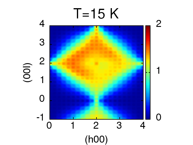
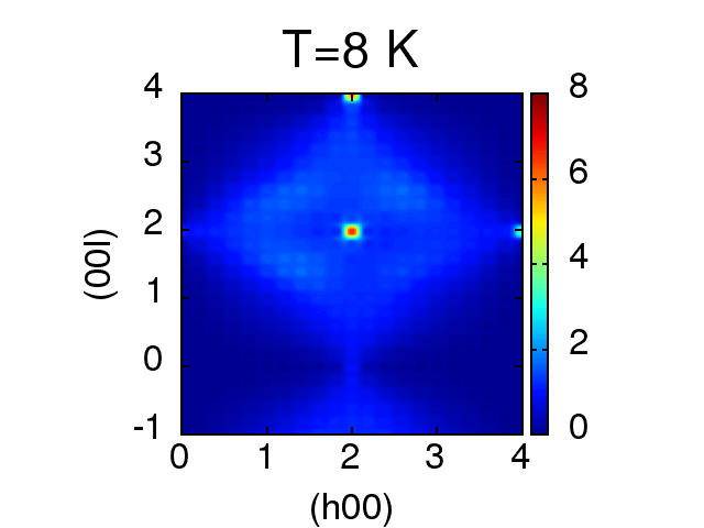
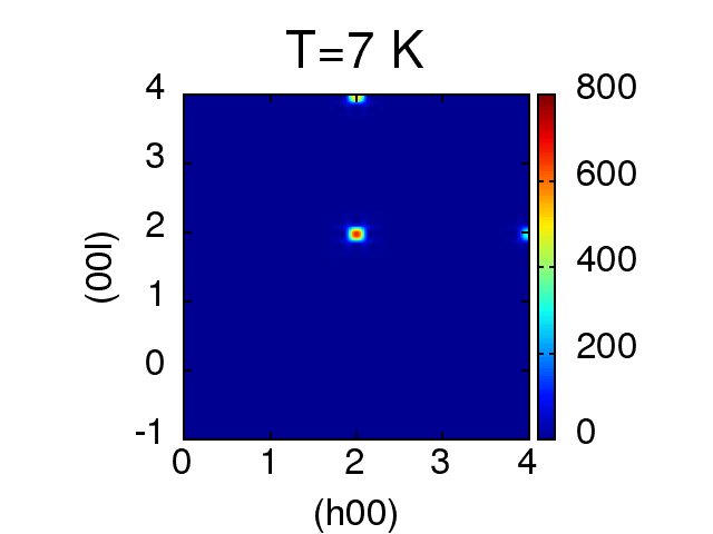
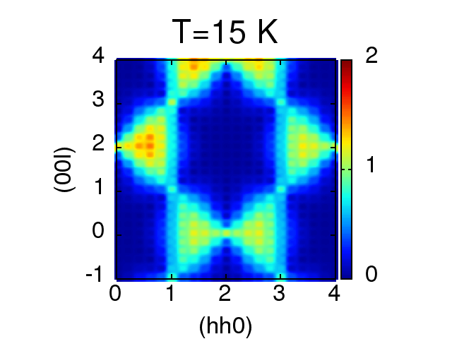
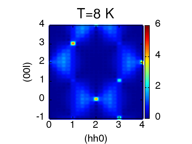
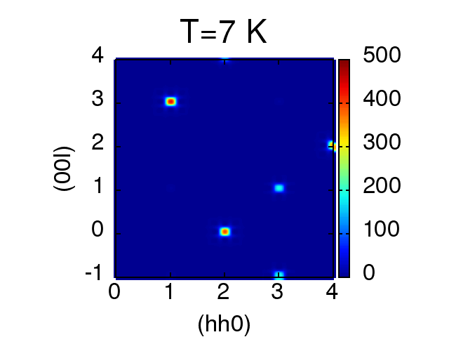
Figure 11: (Color online) The density plot of elastic neutron scattering structure function obtained by MC simulation for $\frac{\Delta V}{V_{0}}=0.15$ at $T=15,8,7$K in a lattice of linear size $L=10$ in (top) : (h0l) planes and (Bottom): (hhl) planes.

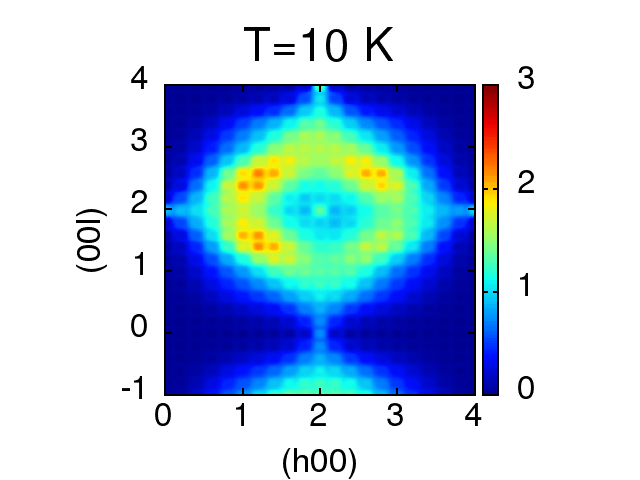
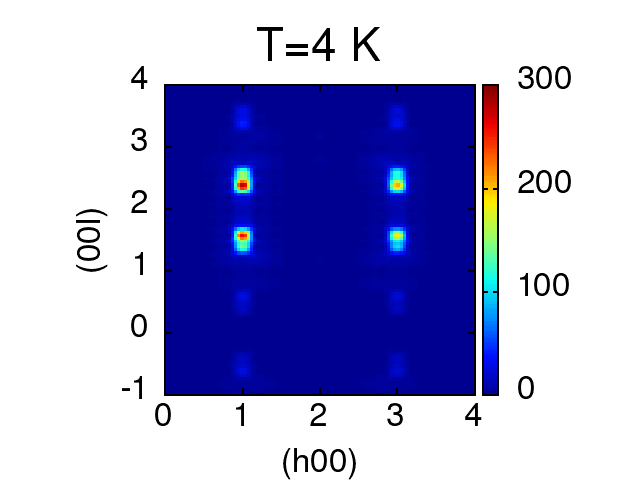
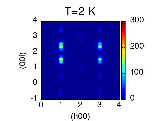
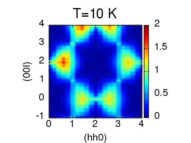
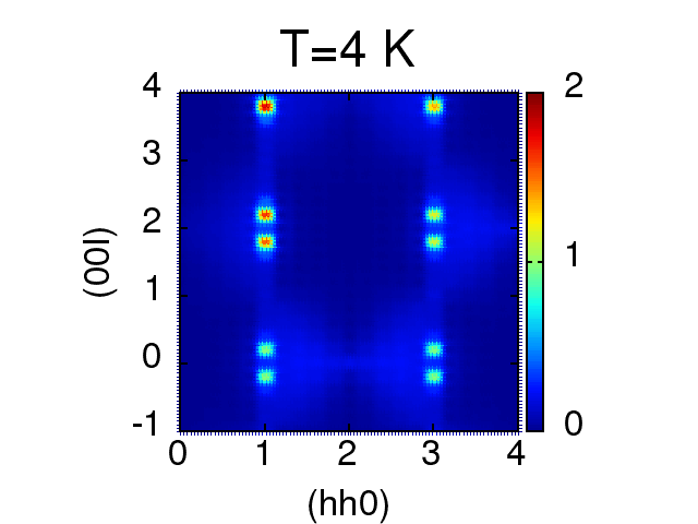
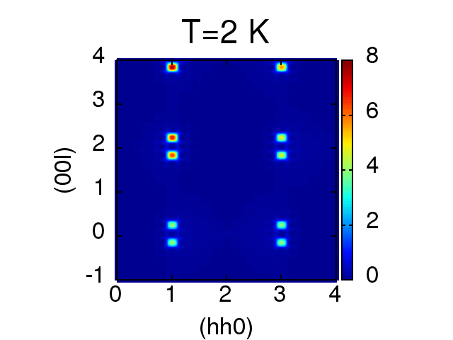
Figure 12: (Color online) The density plot of elastic neutron scattering structure function obtained by MC simulation for $\frac{\Delta V}{V_{0}}=0.2$ at $T=10,4,2$K in a lattice of linear size $L=10$ in (top) : (h0l) planes and (Bottom):(hhl) planes.

The order of transition is determined by the Binder forth energy cumulant given by

$$U(T)=1-\frac{1}{3}\frac{\langle E^{4}\rangle}{\langle E^{2}\rangle^{2}},$$ (2)

in which $E$ is the total energy calculated by MC. For each lattice size, $U(T)$ shows a minimum at the transition temperature depending on the size of the lattice. The value of these minima in three dimensions obeys the following scaling behavior Binder (1981)

$$U_{\rm min}(L)=U^{*}+AL^{-3}+BL^{-6}+O(L^{-9}),$$ (3)

in which $U^{*}$ is the asymptotic value of the minimum of $U(T)$ in the thermodynamic limit. It has been proved Binder (1981) that $U^{*}=2/3$ for the continuous transitions, while for the first order transitions $U^{*}<2/3$. Fig. 9 illustrates the scaling of Binder cumulant minima versus $L^{-3}$ for $\frac{\Delta V}{V_{0}}=-0.05,0.0,0.05$. These results indicate that the order transition changes from first to second at $\frac{\Delta V}{V_{0}}\sim 0.0$. This result suggests that pyr-FeF₃ at the ambient conditions locates in the vicinity of a tricritical point.

Now, we discuss the case of $\frac{\Delta V}{V_{0}}=0.2$. As anticipated, at this volume the system does not exhibit the transition to the AIAO state, however the system undergoes a second order phase transition at $T\sim 4$K. A two dimensional of spin snapshot at $T=0.5$K is illustrated in Fig. 10, showing that the magnetic ground state in this case is spin modulated. To gain more insight into the magnetic ground states of the system we calculate the elastic neutron scattering structure function defined by

$$\begin{split}S(\mathbf{q})=&\sum_{i;j}\langle(\mathbf{S}_{i}-\frac{\mathbf{S}_{i}\bm{\cdot}\mathbf{q}}{\mathbf{q}\bm{\cdot}\mathbf{q}}\mathbf{q})\bm{\cdot}(\mathbf{S}_{j}-\frac{\mathbf{S}_{j}\bm{\cdot}\mathbf{q}}{\mathbf{q}\bm{\cdot}\mathbf{q}}\mathbf{q})\rangle\\ &\exp[i\mathbf{q}\bm{\cdot}(\mathbf{R}_{i}-\mathbf{R}_{j})].\end{split}$$ (4)

The density plots of $S(\mathbf{q})$ for the fractional volume changes $0.15$ and $0.2$ are shown in Figs. 11 and 12, respectively. Both figures show the pinch point structure for $T>T_{C}$ which is a peculiarity of the Coulomb phase in the Hiesenberg antiferromagnets in the pyrochlore lattice. For $\frac{\Delta V}{V_{0}}=0.15$, at $T<T_{C}$ Bragg peaks appears at some pinch points, i.e. $(202),(220),(113)$ which are correspondent to the AIAO spin ordering Sadeghi et al. (2015). However, for $\frac{\Delta V}{V_{0}}=0.2$, the Bragg peaks grow at some non-integer wave vectors, which indicates the transition to a spin modulated state.

III.4 critical exponents

We use the finite-size scaling theoryFisher and Barber (1972); Landau (1976) to find the critical exponents for the second order transitions. The singular parts of the thermodynamic quantities such as, order parameter, AIAO susceptibility and the specific heat are given by

$$m_{n}(t,L) \sim L^{-{\beta}/{\nu}}{\cal F}(tL^{1/\nu})$$ (5)

$$\chi(t,L) \sim L^{\gamma/\nu}{\cal K}(tL^{1/\nu})$$ (6)

$$c(t,L) \sim L^{\alpha/\nu}{\cal C}(tL^{1/\nu}),$$ (7)

where $t=\frac{T_{C}-T}{T_{C}}$ denotes the reduced temperature and $L$ is linear lattice size. The relation between these three exponents are given by the Rushbrooke law Kadanoff et al. (1967) as $\alpha+2\beta+\gamma=2$. Finite-size scaling of the AIAO order parameter for the fractional volume changes $0.0$ and $0.15$ are shown in Fig. 13. This figure clearly shows the data collapse of the different lattice sizes ($L=8,9,10,11$) by choosing $\beta=0.18\pm 0.02$ and $\nu=0.54\pm 0.03$ for $\frac{\Delta V}{V}=0$ and $\beta=0.2\pm 0.02$ and $\nu=0.57\pm 0.06$ for $\frac{\Delta V}{V}=0.15$.

Figure 13: (Color online) Finite-size scaling of the order parameter for (Left)$\frac{\Delta V}{V_{0}}=0$ and (Right) $\frac{\Delta V}{V_{0}}=0.15$.

Figure 14: (Color online) Logarithm of the peaks of specific heat and AIAO susceptibility versus log of the linear size of the lattice ($L=4,5,6,7,8,9,10,11$) for (Top)$\frac{\Delta V}{V_{0}}=0$ and (Bottom) $\frac{\Delta V}{V_{0}}=0.15$.

To obtain the critical exponents $\alpha$ and $\gamma$, we plot the peaks of the specific heat and AIAO susceptibility versus lattice size in log-log scale (see Fig. 14). The best linear fits to these data give rise to $\alpha/\nu=0.89\pm 0.03$ and $\gamma/\nu=1.94\pm 0.01$ for $\frac{\Delta V}{V_{0}}=0.0$ ($\alpha=0.48\pm 0.05$, $\gamma=1.05\pm 0.06$) and $\alpha/\nu=0.85\pm 0.03$ and $\gamma/\nu=1.68\pm 0.09$ for $\frac{\Delta V}{V_{0}}=0.15$ ($\alpha=0.48\pm 0.06$, $\gamma=0.96\pm 0.1$) . It can be easily checked that the calculated exponents $\alpha,\beta$ and $\gamma$ satisfy the Rushbrooke relation in the statistical errors ($\alpha+2\beta+\gamma=1.92+\pm 0.15$ for $\frac{\Delta V}{V_{0}}=0.0$ and $\alpha+2\beta+\gamma=1.85+\pm 0.2$ for $\frac{\Delta V}{V_{0}}=0.15$), moreover, both transitions are in the same universality class. While the exponents $\alpha$ and $\gamma$ are close to the tricritical values ($\alpha=1/2,\gamma=1$), the exponent $\beta$ deviates from the tricritical value $1/4$ which could be due to the closeness of the Lifshitz and tricirtical points in the parameter space of the Hamiltonian. Interestingly, MC results for the Lifshitz point in the antiferromagnetic next to nearest neighbor Ising (ANNNI) model, have given $\beta\sim 0.2$ Selke (1988); Kaski and Selke (1985).

In summery, using DFT calculations we found a spin Hamiltonian for pyr-FeF₃ with different volumes, including a set of coupling constants, i.e. the AF Heisenberg exchange up to the third neighbor, the nearest neighbor bi-quadratic and direct DM interaction. The variation of the coupling constants as the function of volume change are in a way that the spin system shows a first order transition to AIAO for negative volume change with respect to the experimental structure. For the positive volume change we observed a second order transition to AIAO state up to fractional volume change $0.15$, hence suggesting that the spin Hamiltonian corresponding to the experimental structure locates close to a tricritical point. At larger volume changes the system undergoes a transition to a non-uniform spin modulated state. The reason for not having transition to AIAO state for $\frac{\Delta V}{V_{0}}>0.15$ is the sign change of the bi-quadratic coupling ($B$) from positive to negative at $\frac{\Delta V}{V_{0}}\sim 0.15$. In the case that both $B$ and the DM coupling are positive, they cooperate to stabilize the AIAO state at low temperatures Sadeghi et al. (2015). However, when $B$ is negative, this term encourages the collinear state while the DM interaction favors the AIAO, hence the competition between these two gives rise to a modular state. As the conclusion the spin system at $\frac{\Delta V}{V_{0}}=0.15$ is located at the vicinity of a Lifshitz point. Therefore the deviation of the order parameter exponent $\beta$ from the tricritical value can be understood as the crossover from the tricritical point to a nearby lifshitz point.