Does the bottomonium counterpart of $X(3872)$ exist?

Abstract

A narrow line shape peak at about 10615 MeV, just above the threshold in the $B\bar{B}^{*}$ channel, which can be regarded as the signal of bottomonium counterpart of $X(3872)$, $X_{b}$, is predicted by using the extended Friedrichs scheme. Though a virtual state is found at about 10593 MeV in this scheme, we point out that the peak is contributed mainly by the coupling form factor, which comes from the convolution of the interaction term and meson wave functions including the one from $\chi_{b1}(4P)$, but not mainly by the virtual-state pole. In this picture, the reason why $X_{b}$ signal is not observed in the $\Upsilon\pi^{+}\pi^{-}$ and $\Upsilon\pi^{+}\pi^{-}\pi^{0}$ channels can also be understood. The $\chi_{b1}(4P)$ mass and width are found to be about 10771 MeV and 6 MeV, respectively and a dynamically generated broad resonance is also found with its mass and width at about 10672 MeV and 78 MeV, respectively. The line shapes of these two states are also affected by the form factor effect. Thus, this study also emphasizes the importance of the structure of the wave functions of high radial excitations in the analysis of the line shapes, and provides a caveat that some signals may be generated from the structures of the form factors rather than from poles.

Discoveries of the near-threshold exotic states, $X(3872)$ Choi et al. (2003), $Z_{c}$’s Ablikim et al. (2013, 2014), and $Z_{b}$’s Bondar et al. (2012), especially the extremely narrow $X(3872)$, challenge the predictions of the quark model and different models are proposed to understand their masses, as reviewed in Refs. Guo et al. (2018); Chen et al. (2016); Lebed et al. (2017); Esposito et al. (2017). Hadronic molecular states of $D\bar{D}^{*}$ bounded by the long-range force of one pion exchange (OPE), were the first choice of the explanation of these states, proposed even before these states were observed Törnqvist (1991). This idea is generalized from the understanding of the deuteron in the triplet $np$ system Weinberg (1963, 1965). However, this picture meets problems in explaining the production process in hard $p\bar{p}$ collision Acosta et al. (2004); Abazov et al. (2004); Aaij et al. (2012); Bignamini et al. (2009) and the large $\gamma\psi^{\prime}$ decay rate. Another promising approach is to consider the $X(3872)$ as dynamically generated by coupling the $\chi_{c1}(2P)$ and the opened $D\bar{D}^{*}$ continuum Braaten and Lu (2007); Coito et al. (2013); Zhou and Xiao (2017, 2018), which may avoid both problems, and such a picture has attracted more and more interest in the community.

In the bottomonium sector, the $Z_{c}$ counterpart $Z_{b}$’s have already been found, but the bottomonium counterpart of $X(3872)$, dubbed the $X_{b}$ Hou (2006), is still absent in the experimental explorations. The searches for the $X_{b}$ in $\Upsilon\pi^{+}\pi^{-}$ by CMS and ATLAS Chatrchyan et al. (2013); Aad et al. (2015), and in $\Upsilon\pi^{+}\pi^{-}\pi^{0}$ by Belle He et al. (2014) both gave negative results. These results call for a reliable theoretical explanation, and further suggestions of better searching channels are helpful to save the experimental efforts. In the literature, the OPE mechanism was also used in the bottomonium sector and predicts a binding energy of about 42 MeV for the $B\bar{B}^{*}+B^{*}\bar{B}$ system of $J^{PC}=1^{++}$ Tornqvist (1994); Swanson (2006), which means that the bound state is located at about 10562 MeV. The existence of a bound state around the $B\bar{B}^{*}$ threshold was also qualitatively predicted by considering the isospin exchange mechanism in Ref.Karliner and Rosner (2015). In Ref. Karliner and Rosner (2015), the possible mixing between $\chi_{b1}(3P)$ and $X_{b}$ is also discussed. These predictions in the literature all assume the $X_{b}$ to be a bound state of $B\bar{B}^{*}$ by OPE. However, as stated in the previous paragraph, experiments exhibit that the $X(3872)$ contains both $\chi_{c1}(2P)$ and $D\bar{D}^{*}$ components. Thus, to have the same production mechanism as in $X(3872)$, it is more reasonable to couple $\chi_{b1}(4P)$, the nearest $1^{++}$ bottomonium state above the $B\bar{B}^{*}$ threshold, to the opened continua $B\bar{B}^{*}$ and $B^{*}\bar{B}^{*}$.

Motivated by this consideration, we investigate this problem using the extended Friedrichs scheme Xiao and Zhou (2017, 2017, 2016) proposed by us in recent years. The basic idea is as follows. The well-accepted Godfrey-Isgur (GI) model Godfrey and Isgur (1985) can produce the hadron spectra very well below the open-flavor thresholds but cannot describe the states above the threshold well because it does not include the interactions between the hadron states. The Friedrichs model Friedrichs (1948) is an exactly solvable model that couples discrete states and the continuum states, which can be used to take into account the interactions between hadrons. The interactions could not only shift the discrete-state pole to the complex energy plane but also dynamically generate other states. Thus, using the GI’s meson spectra as the inputs and using the widely used quark pair creation (QPC) model to describe the interactions, the Friedrichs model provides a way to incorporate the corrections from formerly neglected interactions in the GI model. This scheme was successfully used in describing the first excited charmonium states with only one free parameter, $\gamma$, the quark pair creation strength. In particular, it generates $X(3872)$ at the experimental value automatically and its wave function can be used to understand the isospin-breaking effects of $X(3872)$ decaying into $J/\psi\pi^{+}\pi^{-}$ and $J/\psi\pi^{+}\pi^{-}\pi^{0}$ Zhou and Xiao (2017, 2018), while the line shape of $D\bar{D}^{*}$ in the $B\to D\bar{D}^{*}K$ process could be reproduced well at the same time. Here, in parallel to the situation in $X(3872)$, using the same $\gamma$ parameter as in the charmonium cases, we couple the $\chi_{b1}(4P)$ to $B\bar{B}^{*}+B^{*}\bar{B}$ and $B^{*}\bar{B}^{*}$ continuum states, and a few interesting results are found as follows. We find that a virtual state is dynamically generated below the $B\bar{B}^{*}$ threshold and the line shape of the $B\bar{B}^{*}$ scattering has a peak structure just above the threshold, which seems to indicate that there is an $X_{b}$ virtual state generating a peak structure. However, by careful analysis, we will show that this peak structure is not contributed mainly by the virtual state but by the form factor in the amplitude. It is reasonable that the form factor which comes from the convolution of the meson wave functions and interaction terms may have nontrivial structures if higher radial excitations with several nodes in the wave functions are included. This picture may also explain why the peak is not seen in the OZI suppressed $\Upsilon\pi^{+}\pi^{-}$ and $\Upsilon\pi^{+}\pi^{-}\pi^{0}$ decay channels. We also show that the line shape of another dynamically generated broad resonance and magnitude of the line shape of a narrow resonance which is originated from the $\chi_{b1}(4P)$ are also largely affected by the structures of the form factors. These results show that when high radial excitations are involved, the effect of the meson structure is important and may even generate peak signals.

Let us first introduce the theoretical background. By extending the well-known Friedrichs model Friedrichs (1948) to the angular momentum eigenstates and restricting it to a specific total angular momentum, the interaction between a discrete state $|0\rangle$ with a bare energy eigenvalue $m_{0}$, and some continuum two-particle states $|E;n,SL\rangle$, where $E$ is the bare energy eigenvalue in the center of mass system (cms) and $n,S$ and $L$ denote the species, total spin and total orbital angular momentum, respectively, can be expressed as a Hamiltonian as Xiao and Zhou (2017, 2017)

$$H= m_{0}|0\rangle\langle 0|+\sum_{n,S,L}\int_{E_{th,n}}^{\infty}\mathrm{d}E\,E|E;n,SL\rangle\langle E;n,SL|\,$$

$$+ \sum_{n,S,L}\int_{E_{th,n}}^{\infty}\mathrm{d}Ef^{n}_{SL}(E)|0\rangle\langle E;n,SL|+H.c.$$ (1)

where ${E_{th,n}}$ is the threshold energy of the $n$th continuum and $f^{n}_{SL}(E)$ represents the coupling form factor of the bare discrete state and the $n$th continuum state. The general eigenvalue problem of Eq. (Does the bottomonium counterpart of $X(3872)$ exist?) could be exactly solved. The bound state, virtual state, and resonance state are determined by the zero points on different Riemann sheets of the inverse of the resolvent, $\eta(z)$, defined as

$$\eta(z)=z-m_{0}-\sum_{n,S,L}\int_{E_{th,n}}^{\infty}\frac{|f^{n}_{SL}(E)|^{2}}{z-E}\mathrm{d}E\,.$$ (2)

Every continuum integral will contribute a discontinuity for the $\eta(z)$ function and doubles the number of Riemann sheets. For example, in a two-channel case, there are two thresholds, $a_{1}$ and $a_{2}$. The physical region between $a_{1}$ and $a_{2}$ is attached to the second sheet, and the physical region above $a_{2}$ is attached to the third Riemann sheet.The zero points of $\eta(z)$ on the unphysical Riemann sheets will be the poles for the $S$ matrix, which represent the generalized eigenstates with complex eigenvalues for the full Hamiltonian, which have rigorous mathematical definition in the rigged Hilbert space Bohm and Gadella (1989); Civitarese and Gadella (2004). The wave functions of such generalized eigenstates could be explicitly written down Xiao and Zhou (2017, 2017) and the scattering matrix element of the initial and final continuum states (the subscripts $i$ and $f$ include their total spin $S$ and angular momentum $L$) could be expressed as

$$S_{fi}(E,E^{\prime})=\delta(E-E^{\prime})\Big{(}\delta_{fi}-2\pi i\frac{f_{i}(E){f_{f}}^{*}(E)}{\eta^{+}(E)}\Big{)},$$ (3)

In general, only the poles on the Riemann sheets closest to the physical region will significantly contribute to the observables such as the cross sections or scattering amplitudes.

A simple method to describe the interaction between one-meson and two-meson continuum states is the QPC model Micu (1969); Blundell and Godfrey (1996), in which the transition operator $T$ of the $A\to BC$ process is defined as

$$T =-3\gamma\sum_{m}\langle 1m1-m|00\rangle\int\mathrm{d}^{3}\vec{p_{3}}\mathrm{d}^{3}\vec{p_{4}}\delta^{3}(\vec{p_{3}}+\vec{p_{4}})$$ (4)

$$\mathcal{Y}_{1}^{m}(\frac{\vec{p_{3}}-\vec{p_{4}}}{2})\chi_{1-m}^{34}\phi_{0}^{34}\omega_{0}^{34}b_{3}^{\dagger}(\vec{p_{3}})d_{4}^{\dagger}(\vec{p_{4}}),$$

describing the process of a quark-antiquark pair being generated by the $b^{\dagger}_{3}$ and $d^{\dagger}_{4}$ creation operators from the vacuum. $\phi_{0}^{34}=(u\bar{u}+d\bar{d}+s\bar{s})/\sqrt{3}$ is the $SU(3)$ flavor wave function for the quark-antiquark pair. $\chi^{34}_{1-m}$ and $\omega^{34}_{0}$ are the spin wave function and the color wave function, respectively. $\mathcal{Y}_{1}^{m}$ is the solid harmonic function. $\gamma$ parametrizes the production strength of the quark-antiquark pair from the vacuum. By the standard derivation and partial wave decomposition one can obtain $f_{SL}(E)$, the coupling form factor between $|A\rangle$ and $|BC\rangle$ in the Friedrichs model Zhou and Xiao (2017).

When the wave functions and the masses of the bare states are given, the form factor $f_{SL}(E)$ can be obtained, and thus, from Eq. (3), the scattering amplitudes of the particular channels can be obtained and the bound states, virtual states or resonant states could be solved from $\eta^{n\mathrm{th}\ \mathrm{sheet}}(z)=0$ on the $n$th Riemann sheet. The $G(z)\equiv f_{i}(z)f_{f}^{*}(z)$ in Eq. (3) will be called the residue function in the following.

We will use the GI model to supply the wave functions and the mass of the bare state, because it has been proved globally successful in predicting meson states below the open-flavor thresholds. The predicted mass of $\chi_{b1}(4P)$ by GI is about 10790 MeV. Since the $B\bar{B}^{*}$ channel threshold is about 10604 MeV and the $B^{*}\bar{B}^{*}$ channel opens above 10649 MeV, it is natural to conjecture that the $\chi_{b1}(4P)$ state will couple to the open $B^{0}\bar{B}^{0*}+H.c.$, $B^{+}\bar{B}^{-*}+H.c.$, and $B^{0*}\bar{B}^{0*}+B^{+*}\bar{B}^{-*}$ channels.

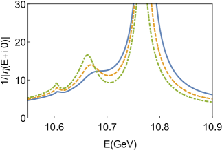
Figure 1: $|\frac{1}{\eta(E+i0)}|$ on the real axis with $\gamma=4.0$(solid line ), 4.9(dashed line), and 5.6(dot-dashed line), respectively.

The wave functions of $B$, $B^{*}$, and $\chi_{b1}(4P)$ could be obtained from the GI model with all the model parameters fixed at their original values Godfrey and Isgur (1985). Then, the only undetermined parameter in our calculation, $\gamma$, is chosen at about $\gamma=4.0$, where the $X(3872)$ and the first excited charmonium states could be reproduced simultaneously Zhou and Xiao (2017, 2018). By solving the zero points of $\eta(z)$, three states are found near the physical region: a virtual-state pole on the second Riemann sheet below the $B\bar{B}^{*}$ threshold at $z_{v}=10593$ MeV, a pair of conjugate poles at $z_{R1}=10771\pm 3i$ MeV on the third Riemann sheet and another pair of third-sheet conjugate poles at $z_{R2}=10672\pm 39i$ MeV. From the curves of $|\frac{1}{\eta({E+i0})}|$ in Fig.1, one can see that the virtual-state pole contributes a small cusp at the $B\bar{B}^{*}$ threshold, while the other two states contribute two peaks around the corresponding energies.

Figure 2: The trajectories of poles on the complex energy plane as $\gamma$ increases. $I$, $II$, and $III$ denote the sheet numbers of the poles as described in the text. Left: $z_{v}$, $z_{R1}$, and $z_{R2}$ with both $B\bar{B}^{*}$ and $B^{*}\bar{B}^{*}$ continua. Right: $z_{R2}^{\prime}$ poles with only the $B^{*}\bar{B}^{*}$.

The origins of these poles could be revealed by tracking their pole trajectories along with the change of $\gamma$, as indicated in Fig. 2. As $\gamma$ becomes smaller, the virtual-state pole $z_{v}$ moves down towards negative infinity on the real axis, remaining as a virtual state. Conversely, if $\gamma$ is turned larger, the virtual state will move up along the real axis and reach the threshold at $\gamma\simeq 8.5$, and then it will come up to the first sheet becoming a bound state. This kind of behavior is the typical behavior for dynamically generated states in $S$ wave with attractive interaction Xiao and Zhou (2016). Therefore, the state can be viewed as dynamically generated mainly from the $S$-wave interaction between the bare $\chi_{b1}(4P)$ state and $B\bar{B}^{*}$ continuum.

Similarly, one could find that $z_{R1}$ is originated from the bare $\chi_{c1}(4P)$ state by turning down the $\gamma$ parameter. $z_{R2}$ is a dynamically generated state mainly from the coupling between $\chi_{b1}(4P)$ and the $B^{*}\bar{B}^{*}$ continuum. This can be demonstrated by switching off only the interaction with the $B\bar{B}^{*}$. Then there is only one cut with two Riemann sheets. As $\gamma$ increases, the $z_{R2}^{\prime}$ poles, which correspond to the third-sheet $z_{R2}$ poles in the two-continuum case, will move towards the $B^{*}\bar{B}^{*}$ threshold, merge at the threshold, and then become a bound-state pole and a virtual-state pole, as shown in the right figure in Fig. 2. This is a typical behavior for dynamically generated states in higher partial waves. Turning on the interaction with $B\bar{B}^{*}$ only modifies this behavior as shown in the left one in Fig. 2. Therefore, we conclude that the $z_{R2}$ is mainly generated from the interaction between $\chi_{b1}(4P)$ and $B^{*}\bar{B}^{*}$. The two dynamically generated states $z_{R2}$ and $z_{v}$ behave differently, because the $S$-wave interaction plays a crucial role in the formation of $z_{v}$ and the $D$-wave interaction is responsible for the formation of $z_{R2}$.

The physical observables are the cross sections, which are related to the continuum scattering amplitudes defined in Eq. (3). The modulus of $B\bar{B}^{*}$ scattering amplitude $|T_{B\bar{B}^{*}\rightarrow B\bar{B}^{*}}|^{2}$ exhibits a very narrow peak in the line shape just above the threshold, as shown in Fig. 3. If this peak is able to be observed in the experiments and its line shape is crudely fitted with a Breit-Wigner formula, it will be concluded that there is a state with a mass about 10615 MeV and a width about 15 MeV by a rough estimation. However, as we have shown, there is no such a zero point of the resolvent function and one can hardly imagine that the virtual state at $z_{v}$, about $10$ MeV below the threshold on the second sheet, can generate such a narrow structure near the threshold. In fact, this line shape peak is mainly contributed by the residue function in Eq. (3), i.e. the $\sum_{SL}|f^{n}_{SL}(E)|^{2}$ terms, but not by the virtual state. This statement can be clarified by comparing the $|1/\eta|$ behavior in Fig. 1 and the residue function behavior in Fig.3. Even when $\gamma$ is increased to about $5.6$ and the virtual-state pole moves to 10600 MeV, its contribution to the threshold enhancement for $|1/\eta|$ is still not significant as shown in Fig. 1. Only if $\gamma$ is tuned up to 8.0, about twice of the original 4.0, when the virtual state comes fairly close to the $B\bar{B}^{*}$ threshold, will its contribution be significant. However, the residue function behavior shown in Fig.3 presents a peak just around the one in $|T|^{2}$. Since the coupling function $f^{n}_{SL}(E)$ in the residue function is obtained from the QPC model, it comes from the convolution of three meson wave functions and the interactions. For mesons with high radial quantum number, such as $\chi_{b1}(4P)$ here, it is well known that there would be several nodes in the radial wave function of the mesons. Therefore, the wavy structures in the residue functions like in $B\bar{B}^{*}$ scattering in Fig. 3 are closely related to the structures in the wave functions of high radial excitations.

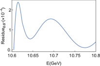
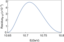
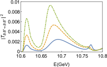
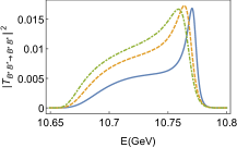
Figure 3: The residue functions of $B\bar{B}^{*}$(left) and $B^{*}\bar{B}^{*}$(right) are shown in the first row. The absolute square of scattering amplitudes of $B\bar{B}^{*}$ and $B^{*}\bar{B}^{*}$ with $\gamma=4.0$(solid), 4.9(dashed line), and 5.6(dot-dashed line ), respectively, are shown in the second row.

In the $B^{*}\bar{B}^{*}$ scattering, $z_{R2}$ and the residue function together will contribute a bump structure, which also appears in the $B\bar{B}^{*}$ scattering. The residue function also plays a role in this structure. The $z_{R2}$ has a broad width of about $78$ MeV at $\gamma=4.0$, which is expected to be a very mild structure. In $B\bar{B}^{*}$ the bump structure around this state is much more obvious than in $B^{*}\bar{B}^{*}$. This is because its position is in a sharply rising part of the residue function in $B\bar{B}^{*}$, being closer to the maximum of the bump in the residue function than in $B^{*}\bar{B}^{*}$, and also because position of the valley of the residue function comes below $z_{R1}$ in $B\bar{B}^{*}$. Thus, this bump structure gets its shape much more from the residue function than from the pole, which can easily be seen by comparing Figs. 1 and 3. Even though the $z_{R1}$ state is a very narrow state which receives less influence from the residue function, a careful observation shows that in the $B\bar{B}^{*}$ channel the position of $\chi_{b1}(4P)$ state is just inside the valley of residue function, and as a result, its maximum contribution in $|T|^{2}$ is comparable to the maximum of the $z_{R2}$ bump, while in $B^{*}\bar{B}^{*}$, its peak is rather sharper and higher compared to the mild structure from $z_{R2}$. This effect is similar to the situation in the $\Upsilon(5S)$ decay Torres-Rincon and Llanes-Estrada (2010)

We also choose another set of meson wave functions, the simple harmonic oscillator functions with the rms radii from the GI model, and found that the line shape structures are almost the same and the above picture is also unchanged.

In this picture, the absence of the $X_{b}$ signal in the $\Upsilon\pi\pi$ channel by CMS and ATLAS Chatrchyan et al. (2013); Aad et al. (2015) and in $\Upsilon\pi\pi\pi$ by Belle He et al. (2014) could be understood. Take the latter for example. If we suppose that the three pions come from $\omega$  and the lower $\Upsilon\omega$ channel is open but coupled weakly, the second-sheet virtual pole will move to the third and fourth sheets, with its mass below the $B\bar{B}^{*}$ threshold. This pole would not affect $1/|\eta|$ significantly in the physical region which is attached to the second sheet below the $B\bar{B}^{*}$ threshold and to the third sheet above the threshold. The residue function of the $\chi_{b1}(4P)$ to $\Upsilon\omega$ is OZI suppressed, and thus, any structure would not be easily observed. So, we suggest further experimental searches could pay more attention to the $B\bar{B}^{*}$ channel, which could be achieved when the SuperKeKB energy is increased Kou et al. (2018).

In summary, we utilize the extended Friedrichs scheme with the wave functions and spectrum from the GI model as input to study the pole structure of $B\bar{B}^{*}$ and $B^{*}\bar{B}^{*}$ scatterings by coupling $\chi_{b1}(4P)$ to $B\bar{B}^{*}$ and $B^{*}\bar{B}^{*}$. It is for the first time that a line shape peak related to the $X_{b}$, at about 10615 MeV, is generated just above the $B\bar{B}^{*}$ threshold and at the same time the $X(3872)$ can be described well in one consistent scheme. In comparison, the tetraquark model could predict an $X_{b}$ state above the $B\bar{B}^{*}$ threshold but cannot describe the mass for $X(3872)$ well Ali et al. (2017). In addition, we have shown that it is the residue functions in the amplitude, which are related to the wave functions of the mesons, rather than the dynamically generated virtual state that contribute to the $X_{b}$ peak dominantly. Our picture could also explain the absence of $X_{b}$ signal evidence in the experiments Chatrchyan et al. (2013); He et al. (2014). A dynamically generated resonance pole is also found at $10672\pm 39i$ MeV and the $\chi_{c1}(4P)$ at $10771\pm 3i$ MeV. The line shapes of these resonances are also affected by the residue functions. In particular, the relative magnitude of the peak generated by the narrow resonance $\chi_{b1}(4P)$ is suppressed by a valley of the residue function. This kind of phenomenon may be a general cause for a state to behave differently in different channels when the form factors are different. In principle, the wave function of a high radial excitation state has a few node structures, and, after being convoluted with the interaction Hamiltonian it may finally cause additional structures of the line shape. This effect is independent of the model chosen in this paper. Thus, the wave functions with higher radial quantum numbers may result in more structures in the line shape. This kind of phenomenon is more or less a model-independent one and should be paid attention to in the theoretical analysis of the line shape data. In comparison, in the effective field theory (EFT) approach, the states are assumed to have no internal structures and the information of the form factors is absorbed into the coupling constants. Therefore, the EFT approach must go to higher orders to reproduce the nontrivial behaviors of the form factors or must include some form factors inserted by hand without any solid theoretical ground, which may constrain the effectiveness of the theory.