Tracking Rydberg atoms with Bose-Einstein Condensates

Abstract

We propose to track position and velocity of mobile Rydberg excited impurity atoms through the elastic interactions of the Rydberg electron with a host condensate. Tracks first occur in the condensate phase, but are then naturally converted to features in the condensate density or momentum distribution. The condensate thus acts analogous to the cloud or bubble chambers in the early days of elementary particle physics. The technique will be useful for exploring Rydberg-Rydberg scattering, rare inelastic processes involving the Rydberg impurities, coherence in Rydberg motion and forces exerted by the condensate on the impurities. Our simulations show that resolvable tracks can be generated within the immersed Rydberg life time and condensate heating is under control. Finally we demonstrate the utility of this Rydberg tracking technique to study ionizing Rydberg collisions or angular momentum changing interactions with the condensate.

I Introduction

Tracking particle motion has helped to advance physics for centuries, in developing Newtonian mechanics, understanding Brownian motion and, more recently, unravelling the standard model of elementary particle physics. Tracks allowed the deduction of fundamental theories through studying the deflection of trajectories by conservative and frictional forces. They further indicate decay products and give clues on particle life-times via track lengths. Early examples of tracking devices were the bubble chamber Glaser (1952) and cloud chamber Gupta and Ghosh (1946), in which an energetic particle leaves an optically visible mark of its passing through interaction with the chamber medium. These devices were later replaced by wire chambers Kleinknecht (1982) and recently silicon detectors Garcia-Sciveres and Wermes (2018).

In ultra-cold atomic physics, about 25 orders of magnitude below the particle physics energy scales, experiments can dope Bose-Einstein condensates (BECs) with impurities such as ions Schmid et al. (2010) or Rydberg atoms Balewski et al. (2013); Schlagmüller et al. (2016); Teixeira et al. (2015). We show that the phase coherence of the BEC allows its use as a tracking instrument for Rydberg impurities, reminiscent of a bubble chamber in the early days of particle physics. Through elastic collisions of the Rydberg electrons with the condensate atoms, tracks are created in the density of the condensate that record Rydberg trajectories and can be detected by in-situ measurements Wilson et al. (2015); Gericke et al. (2008); Hau et al. (1998). Associated phase information also allows to infer Rydberg velocities, and could be read out by interference with a reference condensate Simsarian et al. (2000); Martin and Allen (2007); Meiser and Meystre (2005); Gati et al. (2006); Wang et al. (2005).

Tracking can first verify dipole-dipole and van-der-Waals (vdW) interactions Gallagher (1994); Singer et al. (2005); Weber et al. (2017) of Rydberg atoms, and then explore less well studied inelastic reactions that occur when ground-state atoms interact with Rydberg impurities in the ultracold regime Niederprüm et al. (2015); Balewski et al. (2013); Schlagmüller et al. (2016). While such reactions may somewhat limit BEC in tracking other Rydberg dynamics, they also provide the opportunity to study the timing and evolution during decay processes through the length and features of imprinted tracks.

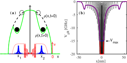
Figure 1: Sketch showing a one-dimensional cut through a Bose-Einstein condensate that is tracking two repelling Rydberg impurities (black $\bullet$). (a) Condensate density $\rho$ before (dashed black line) and after (solid green line) Rydberg motion, with corresponding phase signal (oscillating red line) and sketched Rydberg electron wave-functions (blue bottom near location $x_{1}$ and $x_{2}$). (b) Interaction potential ${V}_{\mbox{\!\! \scriptsize gR}}(\mathbf{R})$ (thin black line) between condensate atoms and a single Rydberg impurity at $x=0$, for principal quantum number $\nu=20$. The classical approximation $V_{c}$ (thick red line) averages over fast oscillations. We also employ the indicated cut-off ${V}_{\mbox{\!\! \scriptsize max}}$ (dotted blue line).

To demonstrate the feasibility of our ideas, we model up to five Rydberg excited atoms mutually interacting via van-der-Waals forces while embedded in a BEC. Rydberg atoms move as in Newton’s equations, while the BEC evolves according to the Gross-Pitaevskii equation including the effect of the impurity potentials Astrakharchik and Pitaevskii (2004); Mukherjee et al. (2015); Shukla et al. (2018). We show that for typical parameters, resolvable phase tracks are obtained within the effective Rydberg life-time Schlagmüller et al. (2016) and find that condensate heating during the tracking process is limited. The classical electron probability distribution in a Rydberg state turns out to be a helpful tool for modelling tracking. Finally we show that the technique can tackle measurements of Rydberg-Rydberg ionization distances and witness angular moment changing processes under realistic conditions.

This article is organized as follows: We introduce our model of a BEC interacting with Rydberg impurities in section II and discuss the basic effect of phase imprinting Mukherjee et al. (2015). We then show in section III that mobile impurities leave behind plenty of tracking information, both in condensate phase and velocity. These simulations benefited from an approximation based on the classical Rydberg electron probability distribution, which we discuss in section IV. We rule out that excess heating would be problematic for scenarios as discussed in section V, and highlight scenarios with detectable slowdown of the impurity by the background condensate in section VI. Applications of Rydberg tracking to the study of exotic atomic physics collisions are suggested in section VII before concluding.

II Interactions between Rydberg impurities and BEC

Consider a Bose-Einstein condensed gas of $N$ Rb⁸⁷ atoms with mass $m$ mostly in their ground state, among which ${N}_{\mbox{\!\! \scriptsize imp}}$ impurity atoms are excited to a Rydberg state $|\,{\Psi}\,\rangle=|\,{\nu s}\,\rangle$, with principal quantum number $\nu\gg 10$ and $l=0$ angular momentum. This is sketched for ${N}_{\mbox{\!\! \scriptsize imp}}=2$ in Fig. 1 (a). We denote the location of impurities with $\mathbf{x}_{n}$. As discussed in Middelkamp et al. (2007); Balewski et al. (2013); Mukherjee et al. (2015); Karpiuk et al. (2015); Shukla et al. (2018), we can then model the BEC in the presence of Rydberg impurities with the Gross-Pitaevskii equation (GPE):

$$i\hbar\frac{\partial}{\partial t}\phi(\mathbf{R})=\bigg{(}-\frac{\hbar^{2}}{2m}\boldsymbol{\nabla}^{2}+W(\mathbf{R})+g_{2D}|\phi(\mathbf{R})|^{2}$$

$$+\sum_{n}^{{N}_{\mbox{\!\! \scriptsize imp}}}V_{0}|\Psi(\mathbf{R}-\mathbf{x}_{n})|^{2}\bigg{)}\phi(\mathbf{R}),$$ (1)

where $\phi(\mathbf{R})$ is the condensate wave function and $W(\mathbf{R})=m\omega_{r}^{2}({x}^{2}+{y}^{2})/2$ describes a two-dimensional (2D) harmonic trap, $\mathbf{R}=[x,y]^{T}$. The third dimension is frozen through tight trapping $\omega_{z}^{2}\gg\omega_{r}$, see e.g. Verma et al. (2017) and Appendix A, hence $g_{2D}=g_{3D}/(\sqrt{2\pi}\sigma_{z})$ describes the effective strength of atomic collisions, where $g_{3D}=4\pi\hbar^{2}a_{s}/m$, with atom-atom s-wave scattering length $a_{s}$ and $\sigma_{z}=\sqrt{\hbar/m\omega_{z}}$.

To formally justify the simple 2D reduction with respect to the Rydberg-BEC interaction we require a scenario as shown in Fig. 2, with the condensate more tightly confined in the z-direction than the Rydberg orbital radius.

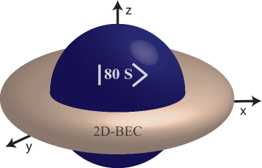
Figure 2: Sketch of Rydberg orbital with larger $z$ extension than the host BEC, justifying to take replace BEC-Rydberg interaction by a 2D cut at $z=0$ through the complete potential.

The last line in (1) represents interactions between the ground state condensate atoms and impurities due to elastic collisions of the Rydberg electron and condensate atoms Greene et al. (2000). The potential for a single impurity ${V}_{\mbox{\!\! \scriptsize gR,n}}(\mathbf{R})\equiv V_{0}|\Psi(\mathbf{R}-\mathbf{x}_{n})|^{2}$, is sketched in Fig. 1 (b). Its strength is set by $V_{0}=2\pi\hbar^{2}a_{e}/m_{e}$ containing the electron-atom scattering length $a_{e}=-16.04a_{0}$, where $a_{0}$ is the Bohr radius foo . The potential shape is set by the Rydberg electron density $|\Psi(\mathbf{R})|^{2}$, where $\Psi(\mathbf{R})=\mbox{$\langle\,{\mathbf{R}}\,|\,{\Psi}\,\rangle$}$.

To describe mobile Rydberg impurities, we couple Eq. (1) to Newton’s equations governing their motion

$$m\frac{\partial^{2}}{\partial t^{2}}\mathbf{x}_{n}=-\mathbf{\nabla_{\mathbf{x}_{n}}}\left[V_{RR}(\mathbf{X})+\bar{V}(\mathbf{x}_{n})\right],$$ (2)

where $V_{RR}(\mathbf{X})=\sum_{n>m}C_{6}(\nu)/|\mathbf{x}_{n}-\mathbf{x}_{m}|^{6}$ is the vdW interaction between Rydberg impurities, with dispersion coefficient $C_{6}$ taken from Singer et al. (2005), and $\mathbf{X}=[\mathbf{x}_{1},\dots,\mathbf{x}_{{N}_{\mbox{\!\! \scriptsize imp}}}]^{T}$ grouping all impurity positions. In addition, the $n^{th}$ impurity feels an effective potential $\bar{V}(\mathbf{x}_{n})=\int d^{2}\mathbf{R}\>\>V_{0}|\Psi(\mathbf{R}-\mathbf{x}_{n})|^{2}|\phi(\mathbf{R})|^{2}$ from the backaction of the condensate Astrakharchik and Pitaevskii (2004); Middelkamp et al. (2007); Shukla et al. (2018). See Appendix A for the 2D reduction.

Let us split the BEC wave function $\phi(\mathbf{R})=\sqrt{\rho(\mathbf{R})}e^{i\varphi(\mathbf{R})}$ into a real density $\rho$ and phase $\varphi$. Then, the initial effect of each impurity is to imprint a phase $\varphi\sim-{V}_{\mbox{\!\! \scriptsize gR,n}}(\mathbf{R})\Delta t/\hbar$, within a short time $\Delta t$ Dobrek et al. (1999); Mukherjee et al. (2015).

II.1 Velocity dependence of phase imprinting

Ignoring all energy contributions except BEC-impurity interaction, for a single impurity with trajectory $\mathbf{x}(t)=\mathbf{v}t$ the solution of Eq. (1) at time $t$ is given by $\phi(\mathbf{R},t)=\phi(\mathbf{R},0)\exp^{i\varphi(\mathbf{R},t)}$, where

$$\varphi(\mathbf{R},t)=-\int dt\>\>V_{0}|\Psi(\mathbf{R}-\mathbf{v}t)|^{2}/\hbar$$ (3)

is the phase imprinted by the moving Rydberg impurities at a location $\mathbf{R}$ in the BEC. Using the definition of a line-integral along the curve $\mathbf{R}^{\prime}=\mathbf{R}-\mathbf{v}t$, we can re-write this as

$$\varphi(\mathbf{R},t)=-\int_{\cal C}dl\>\>V_{0}|\Psi(\mathbf{R}^{\prime}(l))|^{2}/(|\mathbf{v}|\hbar),$$ (4)

where the curve ${\cal C}$ traces the trajectory of the location $\mathbf{R}$ as it moves through the Rydberg electron orbit $\Psi$ in the rest frame of the Rydberg atom. We show Eq. (4) to demonstrate two features: (i) the accumulated phase is a spatial average over $|\Psi|^{2}$ in the direction of motion. As we will show, this allows impurity tracking with the added practical benefit that oscillatory quantum features in Fig. 1 (b) are averaged, so that we can replace ${V}_{\mbox{\!\! \scriptsize gR,n}}(\mathbf{R})$ with a smoother classical approximation ${V}_{\mbox{\!\! \scriptsize c,n}}(\mathbf{R})$ as discussed in section IV. This simplification will be used shortly, in Fig. 3. (ii) The phase is proportional to $|\mathbf{v}|^{-1}$ for uniform motion, and thus contains velocity information.

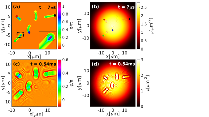
Figure 3: Tracking Rydberg atoms in a BEC through density or phase information. Five $\nu=80$ Rydberg excitations are in a ⁸⁷Rb BEC of $N=1500$ atoms in a $\omega_{r}/(2\pi)=4$ Hz pancake trap, with transverse strength $\omega_{z}/(2\pi)=1$ kHz. (a) Phase imprinted by Rydberg atoms after $t={\tau}_{\mbox{\!\! \scriptsize imp}}=7\mu$s. (b) The density signal at this time is weak. (c,d) Assuming impurities are removed at ${\tau}_{\mbox{\!\! \scriptsize imp}}$, BEC evolution (1) converts the phase signal into clear density signals on the longer time scale ${\tau}_{\mbox{\!\! \scriptsize mov}}=0.54$ ms. See also supplementary movie.

III Phase imprinting versus density modulation

Using XMDS Dennis et al. (2012, 2013), we have numerically solved the coupled system of GPE (1) and Newton’s equations (2) for a comparatively small 2D BEC cloud, with 3D peak density at the centre of $\rho_{0}=4.2\times 10^{18}$ m^-3. Five atoms are excited to $\nu=80$ Rydberg states and placed at $t=0$ initially on the inner starting points of the tracks evident in Fig. 3 (a) . The panel shows the condensate phase $\varphi(\mathbf{R})$. The final position of each atom after an imprinting time ${\tau}_{\mbox{\!\! \scriptsize imp}}=7\mu$s is shown by colored circles with size matching the Rydberg electron orbital radius ${r}_{\mbox{\!\! \scriptsize orb}}=3a_{0}\nu^{2}/2$. Atoms have repelled as in Teixeira et al. (2015), on time-scales very short compared to those typical for BECs. While tracks are clearly visible in the condensate phase, the effect on the density in panel (b) is almost negligible for times as short as ${\tau}_{\mbox{\!\! \scriptsize imp}}$, corresponding to the Raman-Nath regime Müller et al. (2008). The imprinted phase also carries velocity information, since it depends on how long a given location is visited by the impurity as discussed in Sec. II.1. This is shown in the inset of panel (a) for the initial atomic acceleration.

Interferometry can deduce a condensate phase pattern Simsarian et al. (2000); Martin and Allen (2007); Meiser and Meystre (2005); Gati et al. (2006); Wang et al. (2005), but is not commonly available. Fortunately, the phase tracks are converted into density tracks through motion of the ground-state atoms. These have received an initial impulse from the passing Rydberg impurity, causing motion on larger time scales ${\tau}_{\mbox{\!\! \scriptsize mov}}\approx 0.54$ms in panels (c,d). Hence density depressions with $84\%$ contrast appear on either side of the Rydberg track. These can be read out through in-situ density measurements Wilson et al. (2015); Gericke et al. (2008); Hau et al. (1998).

Tracking information is dominated by imprinting via the wide tails of the Rydberg electron density, between $x=10$ and $50$ nm in Fig. 1 (b). We thus cut the large central peak off at ${V}_{\mbox{\!\! \scriptsize max}}$ as shown in blue, to significantly ease simulations. Tracks were largely independent of this technical step, see Fig. 8.

IV Classical electron distribution

To deal with numerical challenges discussed in appendix B, for Fig. 3 we have replaced the potential based on the Rydberg electron wave function ${V}_{\mbox{\!\! \scriptsize gR,n}}(\mathbf{R})$, by one based on the corresponding classical probability density (CPD) Martín-Ruiz et al. (2013):

$$\rho^{\mbox{cl}}(\mathbf{R})=\frac{1}{8\pi^{2}R}\frac{1}{\sqrt{\epsilon^{2}b^{2}-(R-b)^{2}}},$$ (5)

where $R=|\mathbf{R}|$, $b=-k/2E$ is the semi-major axis for the elliptical electron orbit in a Coulomb field $U(\mathbf{R})=-k/{R}$ with $E$ the energy of the $\nu^{th}$ level and $\epsilon=\sqrt{1+2EL^{2}/m_{e}k^{2}}$ the eccentricity. Here $L$ is the angular momentum of the Rydberg state and $m_{e}$ is the mass of the electron.

Overall we thus employ the classical approximation to the Rydberg-BEC interaction potential given by:

$${V}_{\mbox{\!\! \scriptsize c,n}}(\mathbf{R})=V_{0}\begin{cases}\rho^{\mbox{cl}}(\mathbf{R})&R<{R}_{ct},\\ \rho^{Q}(\mathbf{R})&R\geq{R}_{ct}\end{cases},$$ (6)

which is sketched in Fig. 1 (b) as a red line. In (6), ${R}_{ct}=b(1+\epsilon)$ are the classical turning points.

The two potentials give almost identical results as shown for a Rydberg track in Fig. 4. It is created by a single impurity with velocity $v={0.7}$ m/s traversing a homogeneous 2D condensate (${\rho}_{\mbox{\!\! \scriptsize 3D}}=4.2\times 10^{18}m^{-3}$, $\omega_{z}/(2\pi)=1$ kHz). The difference between phases resulting from ${V}_{\mbox{\!\! \scriptsize gR,n}}(\mathbf{R})$ or $V_{c,n}(\mathbf{R})$ is small, see Fig. 4 (b).

This happens, since the motion of the Rydberg impurity causes a local segment of the condensate to feel a spatial average of the electron probability distribution along the direction of motion, see Sec. II.1. According to the correspondence principle, spatially averaging the oscillatory electron density yields the smooth classical probability distribution Martín-Ruiz et al. (2013).

Besides technical utility, this agreement indicates that Rydberg tracking could be used for explorations of the correspondence principle.

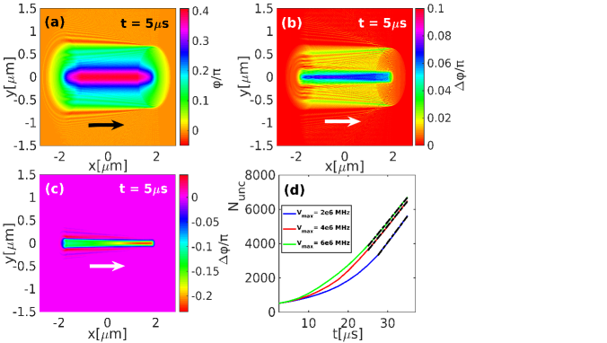
Figure 4: (a) Condensate phase after motion of a single mobile Rydberg impurity in a homogeneous background using the real potential $V_{gR}(\mathbf{R})$, thin black line in Fig. 1 (b). (b) The difference compared to the phases caused by the classical approximation $V_{c}(\mathbf{R})$, red line in Fig. 1 (b), is small. See also supplementary movie. (c) Modifying the potential cut-off only affects the less relevant central part of the track. We show the difference between phases resulting from ${V}_{\mbox{\!\! \scriptsize max}}=2$ MHz and $6$ MHz. (d) Number of un-condensed atoms ${N}_{\mbox{\!\! \scriptsize unc}}$, due to Rydberg impurity determined from the TWA for ${V}_{\mbox{\!\! \scriptsize max}}=2$ MHz, $4$ MHz and $6$ MHz (from bottom line to top line). Dashed lines match the linear rate equation $d{N}_{\mbox{\!\! \scriptsize unc}}/dt=\Gamma$, with $\Gamma\approx 280-300$ atoms$/\mu$s. In contrast, for Fig. 3, heating remains negligible.

V Condensate heating

Experiments report atom-loss and heating when sequentially exciting a large number of Rydberg impurities in a BEC Balewski et al. (2013) . Heating might potentially overwhelm the mechanical effects of Rydberg-BEC interactions that we focus on here. However we now show that heating is limited in our scenarios, since we consider substantially smaller number of Rydberg impurities and shorter times.

For this, we use models beyond the mean-field Eq. (1) using the truncated Wigner approximation (TWA) Steel et al. (1998); Sinatra et al. (2001, 2002); Wüster et al. (2007, 2008); Da̧browska-Wüster et al. (2009); Norrie et al. (2006a). In brief, this adds quantum fluctuations to the initial state of (1) by specific addition of random noise. Averaging over an ensemble of solutions, we can then extract the number of uncondensed atoms ${N}_{\mbox{\!\! \scriptsize unc}}$ from the noise statistics as discussed in the Appendix C. We expect the TWA to give reliable results for the short times ${\tau}_{\mbox{\!\! \scriptsize imp}}$ considered here Polkovnikov (2003).

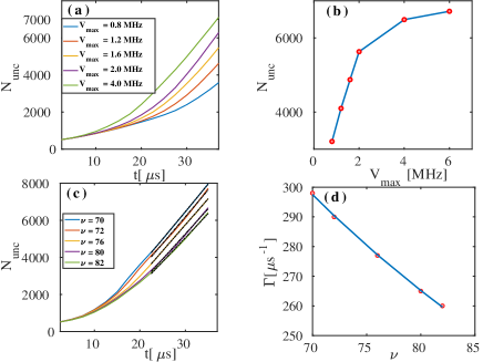
Figure 5: Incoherent response of host Bose-gas to mobile Rydberg impurity. (a) Uncondensed atom number ${N}_{\mbox{\!\! \scriptsize unc}}(t)$, starting from a vacuum state for different ${V}_{\mbox{\!\! \scriptsize max}}$. ${N}_{\mbox{\!\! \scriptsize unc}}$ is increasing for larger ${V}_{\mbox{\!\! \scriptsize max}}$ (from bottom line to top line). The initial total number in the simulation box was $N=70000$ atoms. (b) ${N}_{\mbox{\!\! \scriptsize unc}}(t_{0})$ at a fixed time $t_{0}=35$ $\mu$s as a function of ${V}_{\mbox{\!\! \scriptsize max}}$, showing saturation. (c) The heating actually decreased for increasing principal quantum number $\nu$ (from top line to bottom line). (d) Scaling of final heating rate $\Gamma$ with $\nu$, deduced from linear fits as shown by dashed lines in panel (c).

Under conditions of Fig. 3, we find that up to ${\tau}_{\mbox{\!\! \scriptsize imp}}=7$ $\mu$s while Rydberg atoms exist, they cause only $8$ atoms to become uncondensed. Heating would thus only become significant much later. Thus in Fig. 4d and Fig. 5 we rather show the heating for a single impurity with $v=0.03$m/s traversing a homogeneous 2D condensate ($\rho_{3D}=8.5\times 10^{21}m^{-3}$, $\omega_{z}/(2\pi)=1$kHz).

The uncondensed atom number, ${N}_{\mbox{\!\! \scriptsize unc}}(t)$, increases with time and then typically shows a linear trend after $t\approx 25\mu$s, as shown in Fig. 5a for different potential cut-offs ${V}_{\mbox{\!\! \scriptsize max}}$ at $\nu=80$. We also show in Fig. 5b that the increase in the cut-off ${V}_{\mbox{\!\! \scriptsize max}}$ led to a proportional increase in uncondensed atom number ${N}_{\mbox{\!\! \scriptsize unc}}\propto{V}_{\mbox{\!\! \scriptsize max}}$ at a fixed time ${N}_{\mbox{\!\! \scriptsize unc}}(t_{0})$ until this saturates, with mostly unchanged final heating rates.

The linear increase of ${N}_{\mbox{\!\! \scriptsize unc}}(t)$ at late times in (a) allows the definition of a (final) heating rate $\Gamma$ via

$$\frac{d{N}_{\mbox{\!\! \scriptsize unc}}}{dt}=\Gamma,$$ (7)

as fitted by dashed lines in panel (c) of Fig. 5. We finally show in Fig. 5d that asymptotic heating rates $\Gamma$ scale with the principal quantum number as $\Gamma\sim\nu^{-1}$.

For our 2D TWA calculations we employed $256\times 256$ spatial grid-points, $129\times 129$ Bogoliubov modes with noise and averaged over 30000 trajectories.

Experiments on heating by mobile Rydberg impurities may unravel incoherent versus coherent aspects of impurity-superfluid interactions, involving critical velocities Pethik and Smith (2002), frictional forces Sykes et al. (2009) or Cherenkov radiation Carusotto et al. (2006), all due to the creation of elementary excitations Suzuki (2014).

VI Detection of condensate backaction

We mainly focus on the phase and density tracks imparted by Rydberg impurities on the BEC, however Eq. (1) also includes a backaction of the BEC onto the Rydberg motion: the effective potential in Eq. (2) set by BEC density. This was negligible in Fig. 3 and hence disabled, but can become crucial for denser and smaller condensates (now $N=28000$ atoms with $\omega_{r}/(2\pi)=96$ Hz), shown in Fig. 6. There, just two impurities with $\nu=80$ are initially separated by $d=5.57$ $\mu$m, symmetrically placed on either side of the centre of the condensate, which has a Thomas-Fermi radius ${R}_{\mbox{\!\! \scriptsize TF}}=$ $8.21\mu$m. Rydberg atoms initially accelerate quickly to $v\approx 0.4$ m/s due to vdW repulsion. Once they leave the high density region of the condensate cloud, the attraction to ground-state atoms provided by the Rydberg electron results in an effective potential well $\bar{V}(\mathbf{x}_{n})$, significantly slowing down the Rydberg impurities as shown in panel (a).

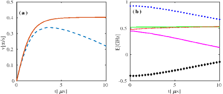
Figure 6: Backaction of condensate background onto dynamic Rydberg atoms. (a) Rydberg velocity as a function of time, with (dashed line) and without (solid line) condensate backaction. (b) Energies with backaction, showing conservation of the total energy ${E}_{\mbox{\!\! \scriptsize tot}}$ (green). Its components, are BEC energy (red dotted), impurity energy (dashed magenta) and BEC-Rydberg interaction energy ${E}_{\mbox{\!\! \scriptsize int}}$ (black $\diamond$). We also show ${E}_{\mbox{\!\! \scriptsize tot}}-{E}_{\mbox{\!\! \scriptsize int}}$ (blue $\bullet$).

Had we not included this force in the simulation, the total energy would not be conserved as shown in panel (b). This total energy of the complete system (Rydberg + BEC) is given by $E={E}_{\mbox{\!\! \scriptsize Ryd}}+{E}_{\mbox{\!\! \scriptsize BEC}}+{E}_{\mbox{\!\! \scriptsize int}}$. Here ${E}_{\mbox{\!\! \scriptsize Ryd}}$ is the total energy of the Rydberg impurities

$${E}_{\mbox{\!\! \scriptsize Ryd}} =V_{RR}(\mathbf{X})+\sum_{n}^{{N}_{\mbox{\!\! \scriptsize imp}}}\frac{1}{2}m\mathbf{v}_{n}^{2},$$ (8)

where $\mathbf{v}_{n}$ is the velocity of impurity $n$. The total energy of the BEC is given by the Gross-Pitaevskii energy functional,

$${E}_{\mbox{\!\! \scriptsize BEC}} =\int d^{2}\mathbf{R}\>\>\phi^{*}(\mathbf{R})\bigg{(}-\frac{\hbar^{2}}{2m}\boldsymbol{\nabla}^{2}+W(\mathbf{R})$$

$$+g_{2D}|\phi(\mathbf{R})|^{2}\bigg{)}\phi(\mathbf{R}).$$ (9)

The interaction energy due to Rydberg-BEC interaction potential ($V_{gR}$) is

$${E}_{\mbox{\!\! \scriptsize int}} =\sum_{n}\int d^{2}\mathbf{R}\>\>V_{0}|\Psi(\mathbf{R}-\mathbf{x}_{n})|^{2}|\phi(\mathbf{R})|^{2}.$$ (10)

The backaction effect in Fig. 6 should be observable in experiment, using tracking or conventional techniques.

VII Tracking Rydberg scattering processes

Figure 7: Condensate tracking of ultra cold Rydberg processes, see also movies: (a) top: Ionizing attractive collision of Rydberg atoms in states $|\,{\nu=80,l=2,m=2}\,\rangle$ for quantisation axis along $y$. We assume instant ionization at ${d}_{\mbox{\!\! \scriptsize ion}}=5$ $\mu$m and included ${\sigma}_{\mbox{\!\! \scriptsize opt}}=0.5$ $\mu$m optical resolution, see Appendix D. bottom: atoms in the same states but moving repulsively. (b) Angular momentum $l$-changing collision with a background atom from $l=0$ to $l^{\prime}=1$ at the white dashed line, clearly changing the character of the track.

Our simulation in Fig. 3 demonstrates that kinematic data of mobile Rydberg impurities can be viably extracted through their interaction with a host BEC, mimicking particle physics tracking techniques. Importantly, the required motional time ${\tau}_{\mbox{\!\! \scriptsize imp}}=7\mu$s is within the life-time $\tau\approx 40\mu$s$/{N}_{\mbox{\!\! \scriptsize imp}}$= $8\mu$s of all five atoms expected based on Schlagmüller et al. (2016) within the condensate. However at $t=7\mu$s we would already frequently expect to see a Rydberg atom that experienced an inelastic interaction with the BEC, such as a change of the angular momentum state of the atom Schlagmüller et al. (2016). Our technique now opens a window on such ultracold quantum dynamical processes. We demonstrate the tracking of two of these in Fig. 7. Panel (a) shows that terminating tracks allow us to infer the ionization distance ${d}_{\mbox{\!\! \scriptsize ion}}$ of two attractively interacting Rydberg atoms Li et al. (2005); Amthor et al. (2007); Viteau et al. (2008); Park et al. (2011) even with finite optical resolution. We have assumed an ${\cal E}\approx 1$ V/cm extraction field along $z$, such that the ionized electron would leave the BEC within $1$ ns. The panel also illustrates that the observed pattern could discriminate repulsive and attractive motion even for the same Rydberg states . Panel (b) shows the track of a single Rydberg atom which experiences an instantaneous angular momentum $l$-changing collision Schlagmüller et al. (2016) with a condensate atom at the indicated point. Since the imprinting signature depends on $l$ Karpiuk et al. (2015), we can infer the location of the event.

Such measurements can then help to develop theory for Rydberg-Rydberg ionization dynamics or angular momentum evolution in the presence of a continuous measurement, which is not fully established at this stage.

VIII Conclusions

Mobile Rydberg atoms can be tracked through density depressions they cause while passing through a BEC. Modelling this is greatly facilitated by approximating the Rydberg-BEC potential using the classical electron position distribution. On the short time scales required for the tracking, heating and inelastic decay are under control. We demonstrate that BEC based Rydberg tracking can help advance our understanding of ultracold quantum dynamical processes, such as ionization and state changing collisions. Other effects explorable may include phonon mediated Rydberg-Rydberg interactions Wang et al. (2015), damping of Rydberg motion Ostmann and Strunz (2017) and decoherence of multiple excitonic Born-Oppenheimer surfaces Wüster and Rost (2018). The latter can provide directed energy transport Wüster et al. (2010); Möbius et al. (2011) or conical intersections Wüster et al. (2011); K Leonhardt and S Wüster and J.-M. Rost (2014); Leonhardt et al. (2017). Tracking enables detection of such effects, and will introduce a well defined decoherence channel akin to the discussion of Wüster (2017).

All phenomena discussed here should remain qualitatively unchanged if the direct Rydberg-electron-BEC interaction is replaced with dressed impurity-BEC long range interactions discussed in Mukherjee et al. (2015). This turns the range of the imprinting potential and thus the width of tracks into a tuneable parameter.

Appendix A Dimensionality reduction for Gross-Pitaevskii equation

The main article employs a GPE in two spatial dimensions, which eases simulations and in an experiment would ease detection. Let us briefly discuss the approximations that allow the reduction of the 3D GPE to a 2D GPE. The evolution of BEC in the presence of a Rydberg impurity in 3D is governed by:

$$i\hbar\frac{\partial}{\partial t}\phi(\tilde{\mathbf{R}})=\bigg{(}-\frac{\hbar^{2}}{2m}\boldsymbol{\nabla}_{\tilde{\mathbf{R}}}^{2}+W(\tilde{\mathbf{R}})+g_{3D}|\phi(\tilde{\mathbf{R}})|^{2}$$

$$+\sum_{n}^{{N}_{\mbox{\!\! \scriptsize imp}}}V_{0}|\Psi(\tilde{\mathbf{R}}-\tilde{\mathbf{x}}_{n})|^{2}\bigg{)}\phi(\tilde{\mathbf{R}}),$$ (11)

where $W(\tilde{\mathbf{R}})=m(\omega_{r}^{2}(x^{2}+y^{2})+\omega_{z}^{2}z^{2})/2$ is the 3D harmonic potential and $\tilde{\mathbf{R}}=[x,y,z]^{T}$ is the 3D coordinate vector. We take $\omega_{z}\gg\omega_{r}$ and assume the wavefunction $\phi(\tilde{\mathbf{R}})$ factors into a part for the in plane coordinate ($\mathbf{R}=[x,y]^{T}$) and a part for the z-direction as, $\phi(\tilde{\mathbf{R}},t)=\phi(\mathbf{R},t)\phi(z)$. Importantly $\phi(z)$ is frozen in the harmonic oscillator ground state along $z$, normalized to unity. After multiplying by $\phi^{*}(z)$ and integrating (11) here along the $z$-direction we obtain Eq. (1) of the main article, which effectively describes a tightly trapped pancake BEC. We consider parameters for which $\sigma_{z}=0.3$ $\mu$m $<{r}_{\mbox{\!\! \scriptsize orb}}=0.6$ $\mu$m. We can thus assume the Rydberg wave-function does not vary significantly over the range of $z$ with non-vanishing BEC, see Fig. 2. Then, during the 3D$\rightarrow$2D reduction, we can approximate:

$$\int dz\>\>V_{0}|\Psi(\tilde{\mathbf{R}}-\mathbf{x}_{n})|^{2}|\phi(z)|^{2}$$ (12)

$$\approx\>\>V_{0}|\Psi(\mathbf{R}-\mathbf{x}_{n})|^{2}\int dz|\phi(z)|^{2}=V_{0}|\Psi(\mathbf{R}-\mathbf{x}_{n})|^{2}.$$

Effectively, in Eq. (12), we thus only use a 2D cut at $z=0$ through the effective potential ${V}_{\mbox{\!\! \scriptsize gR,n}}(\mathbf{R})$, as shown in Fig. 2.

Appendix B Quantum versus classical Rydberg electron probability distributions

The Rydberg-condensate interaction potential (${V}_{\mbox{\!\! \scriptsize gR}}$) contains a 2D cut of the quantum probability density (QPD), $\rho^{Q}(\mathbf{R})=|\Psi(|\mathbf{R}|)|^{2}$ (for a single impurity at $\mathbf{x}=0)$. Modelling the ensuing BEC dynamics encounters two major computational challenges: (i) Resolving the highly oscillatory Rydberg wave function in Fig. 1 (b) on nm scales, while spanning the whole host BEC of radius $\sim 20$ $\mu$m necessitates a very large number of discrete spatial points. (ii) At the same time, very short time steps are forced by large interaction energies ${\cal O}$(10 GHz) of ground-state and Rydberg atoms near the Rydberg core only. We tackle the former point (i) by replacing the QPD in Eq. (1) by the classical probability density (CPD) Martín-Ruiz et al. (2013) in Eq. (5).

The CPD becomes ill defined after the outer classical turning point ${R}_{ct}$, where ${R}_{ct}=b(1+\epsilon)$. Therefore, for $R>R_{ct}$ we revert from (5) back to the tail of the QPD for a smooth and well approximated distribution, as listed in Eq. (6).

We solve problem (ii) by using a high-energy cutoff at $|V(\mathbf{R})|={V}_{\mbox{\!\! \scriptsize max}}$. Due to the minor spatial extent of the potential region affected by the cut-off, its impact on our results is small. This is seen by comparing Fig. 8 here with Fig. 3 of the main article.

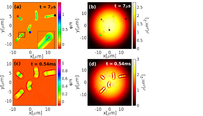
Figure 8: The same as Fig. 3 of the main article but using the cutoff ${V}_{\mbox{\!\! \scriptsize max}}=20$ MHz instead of $2$ MHz.

Appendix C Truncated Wigner approximation

After its introduction to BEC Steel et al. (1998); Sinatra et al. (2001, 2002) the TWA in a BEC context is described in many articles including the review Blakie et al. (2008). The central ingredient of the method is adding random noise to the initial state of the GPE, Eq. (1) of the main article, in order to provide an estimate for the effects of quantum depletion or thermal fluctuations beyond the mean field. We thus use the initial stochastic field

$$\alpha(\mathbf{R},0) =\phi_{0}+\sum_{k}[\eta_{k}u_{k}(\mathbf{R})-\eta^{*}_{k}v^{*}_{k}(\mathbf{R})]/\sqrt{2}.$$ (13)

with random complex Gaussian noises $\eta_{k}$ fulfilling $\overline{\eta_{k}\eta_{l}}=0$ and $\overline{\eta_{k}\eta^{*}_{l}}=\delta_{nl}$, where $\overline{\dots}\mbox{ }$ is a stochastic average. $u_{k}(\mathbf{R})$ and $v_{k}(\mathbf{R})$ are the usual (2D) Bogoliubov modes in a homogenous BEC with density $\rho=|\phi_{0}|^{2}$ Pethik and Smith (2002).

A different symbol $\alpha(\mathbf{R})$ has been chosen for the stochastic field compared to the mean field $\phi(\mathbf{R})$, to emphasise the difference in physical interpretation due to the presence of noise: The stochastic field now allows the approximate extraction of quantum correlations using the prescription

$$\frac{1}{2}\big{(}\langle\hat{\Psi}^{\dagger}(\mathbf{R}^{\prime})\hat{\Psi}(\mathbf{R})\rangle+\langle\hat{\Psi}(\mathbf{R})\hat{\Psi}^{\dagger}(\mathbf{R}^{\prime})\rangle\big{)}\rightarrow\overline{\alpha^{*}(\mathbf{R}^{\prime})\alpha(\mathbf{R})}$$ (14)

Using restricted basis commutators $\delta_{c}$ Norrie et al. (2006b); Norrie (2005), we can then extract the total atom density

$${n}_{\mbox{\!\! \scriptsize tot}}(\mathbf{R}) =\overline{|\alpha(\mathbf{R})|^{2}}-\frac{\delta_{c}}{2},$$ (15)

condensate density ${n}_{\mbox{\!\! \scriptsize cond}}(\mathbf{R})=\left|\overline{\alpha(\mathbf{R})}\right|^{2}$ and from these both the uncondensed density ${n}_{\mbox{\!\! \scriptsize unc}}(\mathbf{R})={n}_{\mbox{\!\! \scriptsize tot}}(\mathbf{R})-{n}_{\mbox{\!\! \scriptsize cond}}(\mathbf{R})$, see also Wüster et al. (2007, 2008); Da̧browska-Wüster et al. (2009). Uncondensed atom numbers as a measure of non-equilibrium“heating” referred to in the main article are finally ${N}_{\mbox{\!\! \scriptsize unc}}=\int d^{2}\mathbf{R}\>{n}_{\mbox{\!\! \scriptsize unc}}(\mathbf{R})$.

Appendix D Finite experimental resolution

To assess the feasibility to directly detect features presented here with in-situ condensate imaging Wilson et al. (2015); Gericke et al. (2008); Hau et al. (1998), we have calculated a density signal at finite resolution ${\rho}_{\mbox{\!\! \scriptsize sig}}(\mathbf{R})$ by convolution of density data with a Gaussian point spread function

$${\rho}_{\mbox{\!\! \scriptsize sig}}(\mathbf{R})={\cal N}\int d^{2}\mathbf{R^{\prime}}e^{-2(|\mathbf{R}-\mathbf{R^{\prime}}|^{2}/{\sigma}_{\mbox{\!\! \scriptsize\tiny opt}}^{2})}|\phi(\mathbf{R^{\prime}})|^{2},$$ (16)

where ${\sigma}_{\mbox{\!\! \scriptsize opt}}$ is the optical resolution and ${\cal N}$ normalizes the Gaussian to one.

Density tracks as shown in Fig. 3 of the main article can be seen with ${\sigma}_{\mbox{\!\! \scriptsize opt}}=0.5\mu$m, challenging but still above the diffraction limit. This is demonstrated in Fig. 9 here.

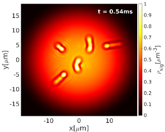
Figure 9: The same as Fig. 3d of the main article but assuming an optical resolution ${\sigma}_{\mbox{\!\! \scriptsize opt}}=0.5\mu m$ as used for Fig. 7 of the main article.

Since the trackable ultra cold dynamics processes in Fig. 7 of the main article were already shown with finite resolution, we included the raw simulation data in Fig. 10.

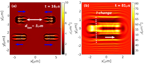
Figure 10: The same as Fig. 7 of the main article but without finite resolution effects.

References

- Glaser (1952) D. A. Glaser, Phys. Rev. 87, 665 (1952).
- Gupta and Ghosh (1946) N. N. D. Gupta and S. K. Ghosh, Rev. Mod. Phys. 18, 225 (1946).
- Kleinknecht (1982) K. Kleinknecht, Phys. Rep. 84, 85 (1982).
- Garcia-Sciveres and Wermes (2018) M. Garcia-Sciveres and N. Wermes, Reports on Progress in Physics 81, 066101 (2018).
- Schmid et al. (2010) S. Schmid, A. Härter, and J. H. Denschlag, Phys. Rev. Lett. 105, 133202 (2010).
- Balewski et al. (2013) J. B. Balewski, A. T. Krupp, A. Gaj, D. Peter, H. P. Büchler, R. Löw, S. Hofferberth, and T. Pfau, Nature 502, 664 (2013).
- Schlagmüller et al. (2016) M. Schlagmüller, T. C. Liebisch, F. Engel, K. S. Kleinbach, F. Böttcher, U. Hermann, K. M. Westphal, A. Gaj, R. Löw, S. Hofferberth, et al., Phys. Rev. X 6, 031020 (2016).
- Teixeira et al. (2015) R. C. Teixeira, C. Hermann-Avigliano, T. L. Nguyen, T. Cantat-Moltrecht, J. M. Raimond, S. Haroche, S. Gleyzes, and M. Brune, Phys. Rev. Lett. 115, 013001 (2015).
- Wilson et al. (2015) K. E. Wilson, Z. L. Newman, J. D. Lowney, and B. P. Anderson, Phys. Rev. A 91, 023621 (2015).
- Gericke et al. (2008) T. Gericke, P. Würtz, D. Reitz, T. Langen, and H. Ott, Nature Physics 4, 949 EP (2008).
- Hau et al. (1998) L. V. Hau, B. D. Busch, C. Liu, Z. Dutton, M. M. Burns, and J. A. Golovchenko, Phys. Rev. A 58, R54 (1998).
- Simsarian et al. (2000) J. E. Simsarian, J. Denschlag, M. Edwards, C. W. Clark, L. Deng, E. W. Hagley, K. Helmerson, S. L. Rolston, and W. D. Phillips, Phys. Rev. Lett. 85, 2040 (2000).
- Martin and Allen (2007) A. V. Martin and L. J. Allen, Phys. Rev. A 76, 053606 (2007).
- Meiser and Meystre (2005) D. Meiser and P. Meystre, Phys. Rev. A 72, 023605 (2005).
- Gati et al. (2006) R. Gati, B. Hemmerling, J. Fölling, M. Albiez, and M. K. Oberthaler, Phys. Rev. Lett. 96, 130404 (2006).
- Wang et al. (2005) Y.-J. Wang, D. Z. Anderson, V. M. Bright, E. A. Cornell, Q. Diot, T. Kishimoto, M. Prentiss, R. A. Saravanan, S. R. Segal, and S. Wu, Phys. Rev. Lett. 94, 090405 (2005).
- Gallagher (1994) T. F. Gallagher, Rydberg Atoms (Cambridge University Press, Cambridge, 1994).
- Singer et al. (2005) K. Singer, J. Stanojevic, M. Weidemüller, and R. Côté, J. Phys. B 38, S295 (2005).
- Weber et al. (2017) S. Weber, C. Tresp, H. Menke, A. Urvoy, O. Firstenberg, H. P. Büchler, and S. Hofferberth, J. Phys. B 50, 133001 (2017).
- Niederprüm et al. (2015) T. Niederprüm, O. Thomas, T. Manthey, T. M. Weber, and H. Ott, Phys. Rev. Lett. 115, 013003 (2015).
- Astrakharchik and Pitaevskii (2004) G. E. Astrakharchik and L. P. Pitaevskii, Phys. Rev. A 70, 013608 (2004).
- Mukherjee et al. (2015) R. Mukherjee, C. Ates, Weibin Li, and S. Wüster, Phys. Rev. Lett. 115, 040401 (2015).
- Shukla et al. (2018) V. Shukla, R. Pandit, and M. Brachet, Phys. Rev. A 97, 013627 (2018).
- Middelkamp et al. (2007) S. Middelkamp, I. Lesanovsky, and P. Schmelcher, Phys. Rev. A 76, 022507 (2007).
- Karpiuk et al. (2015) T. Karpiuk, M. Brewczyk, K. Ra̧żewski, A. Gaj, J. B. Balewski, A. T. Krupp, M. Schlagmüller, R. Löw, S. Hofferberth, and T. Pfau, New J. Phys. 17, 053046 (2015).
- Verma et al. (2017) G. Verma, U. D. Rapol, and R. Nath, Phys. Rev. A 95, 043618 (2017).
- Greene et al. (2000) C. H. Greene, A. S. Dickinson, and H. R. Sadeghpour, Phys. Rev. Lett. 85, 2458 (2000).
- (28) We neglect the dependence of on electron momentum for simplicity.
- Dobrek et al. (1999) Ł. Dobrek, M. Gajda, M. Lewenstein, K. Sengstock, G. Birkl, and W. Ertmer, Phys. Rev. A 60, R3381 (1999).
- Dennis et al. (2012) G. R. Dennis, J. J. Hope, and M. T. Johnsson (2012), http://www.xmds.org/.
- Dennis et al. (2013) G. R. Dennis, J. J. Hope, and M. T. Johnsson, Comput. Phys. Comm. 184, 201 (2013).
- Müller et al. (2008) H. Müller, S.-w. Chiow, and S. Chu, Phys. Rev. A 77, 023609 (2008).
- Martín-Ruiz et al. (2013) A. Martín-Ruiz, J. Bernal, A. Frank, and A. Carbajal-Dominguez, Journal of Modern Physics 4, 818 (2013).
- Steel et al. (1998) M. J. Steel, M. K. Olsen, L. I. Plimak, P. D. Drummond, S. M. Tan, M. J. Collett, D. F. Walls, and R. Graham, Phys. Rev. A 58, 4824 (1998).
- Sinatra et al. (2001) A. Sinatra, C. Lobo, and Y. Castin, Phys. Rev. Lett. 87, 210404 (2001).
- Sinatra et al. (2002) A. Sinatra, C. Lobo, and Y. Castin, J. Phys. B 35, 3599 (2002).
- Wüster et al. (2007) S. Wüster, B. J. Da̧browska-Wüster, A. S. Bradley, M. J. Davis, P. B. Blakie, J. J. Hope, and C. M. Savage, Phys. Rev. A 75, 043611 (2007).
- Wüster et al. (2008) S. Wüster, B. J. Da̧browska-Wüster, S. M. Scott, J. D. Close, and C. M. Savage, Phys. Rev. A 77, 023619 (2008).
- Da̧browska-Wüster et al. (2009) B. J. Da̧browska-Wüster, S. Wüster, and M. J. Davis, New J. Phys. 11, 053017 (2009).
- Norrie et al. (2006a) A. A. Norrie, R. J. Ballagh, C. W. Gardiner, and A. S. Bradley, Phys. Rev. A 73, 043618 (2006a).
- Polkovnikov (2003) A. Polkovnikov, Phys. Rev. A 68, 053604 (2003).
- Pethik and Smith (2002) C. J. Pethik and H. Smith, Bose-Einstein condensation in dilute gases (Cambridge University Press, 2002).
- Sykes et al. (2009) A. G. Sykes, M. J. Davis, and D. C. Roberts, Phys. Rev. Lett. 103, 085302 (2009).
- Carusotto et al. (2006) I. Carusotto, S. X. Hu, L. A. Collins, and A. Smerzi, Phys. Rev. Lett. 97, 260403 (2006).
- Suzuki (2014) J. Suzuki, Phys. A 397, 40 (2014).
- Li et al. (2005) W. Li, P. J. Tanner, and T. F. Gallagher, Phys. Rev. Lett. 94, 173001 (2005).
- Amthor et al. (2007) T. Amthor, M. Reetz-Lamour, S. Westermann, J. Denskat, and M. Weidemüller, Phys. Rev. Lett. 98, 023004 (2007).
- Viteau et al. (2008) M. Viteau, A. Chotia, D. Comparat, D. A. Tate, T. F. Gallagher, and P. Pillet, Phys. Rev. A 78, 040704 (2008).
- Park et al. (2011) H. Park, E. S. Shuman, and T. F. Gallagher, Phys. Rev. A 84, 052708 (2011).
- Wang et al. (2015) J. Wang, M. Gacesa, and R. Côté, Phys. Rev. Lett. 114, 243003 (2015).
- Ostmann and Strunz (2017) P. Ostmann and W. T. Strunz (2017), eprint https://arxiv.org/abs/1707.05257.
- Wüster and Rost (2018) S. Wüster and J. M. Rost, J. Phys. B 51, 032001 (2018).
- Wüster et al. (2010) S. Wüster, C. Ates, A. Eisfeld, and J. M. Rost, Phys. Rev. Lett. 105, 053004 (2010).
- Möbius et al. (2011) S. Möbius, S. Wüster, C. Ates, A. Eisfeld, and J. M. Rost, J. Phys. B 44, 184011 (2011).
- Wüster et al. (2011) S. Wüster, A. Eisfeld, and J. M. Rost, Phys. Rev. Lett. 106, 153002 (2011).
- K Leonhardt and S Wüster and J.-M. Rost (2014) K Leonhardt and S Wüster and J.-M. Rost, Phys. Rev. Lett. 113, 223001 (2014).
- Leonhardt et al. (2017) K. Leonhardt, S. Wüster, and J. M. Rost, J. Phys. B 50, 054001 (2017).
- Wüster (2017) S. Wüster, Phys. Rev. Lett. 119, 013001 (2017).
- Blakie et al. (2008) P. Blakie, A. Bradley, M. Davis, R. Ballagh, and C. Gardiner, Advances in Physics 57, 363 (2008).
- Norrie et al. (2006b) A. A. Norrie, R. J. Ballagh, and C. W. Gardiner, Phys. Rev. A 73, 043617 (2006b).
- Norrie (2005) A. A. Norrie, Ph.D. thesis, University of Otago (2005), URL http://www.physics.otago.ac.nz/nx/jdc/jdc-thesis-page.html.