Unique Metric for Health Analysis with Optimization of Clustering Activity and Cross Comparison of Results from Different Approach

Kumarjit Pathak Kumarjit.pathak@outlook.com Jitin Kapila Jitin.kapila@outlook.com Data Science Researchers, Bangalore, India

Abstract

In machine learning and data mining, Cluster analysis is one of the most widely used unsupervised learning technique. Philosophy of this algorithm is to find similar data items and group them together based on any distance function in multidimensional space. These methods are suitable for finding groups of data that behave in a coherent fashion. The perspective may vary for clustering i.e. the way we want to find similarity, some methods are based on distance such as K-Means technique and some are probability based, like GMM. Understanding prominent segment of data is always challenging as multidimension space does not allow us to have a look and feel of the distance or any visual context on the health of the clustering.

While explaining data using clusters, the major problem is to tell how many cluster are good enough to explain the data. Generally basic descriptive statistics are used to estimate cluster behaviour like scree plot, dendrogram etc. We propose a novel method to understand the cluster behaviour which can be used not only to find right number of clusters but can also be used to access the difference of health between different clustering methods on same data. Our technique would also help to also eliminate the noisy variables and optimize the clustering result.

1. Introduction

Unsupervised learning is part of machine learning, where the objective of the methods is to understand the patterns or classes without any supervision or pre-defined labels. Clustering techniques are few of the important methods to achieve these objectives. In last few decades there has been great momentum in using and advancing these methods to make sense from the data.

These methods proved to be a great tool for understanding and creating groups of coherent behaviours within the data. Immense business importance of these unsupervised techniques has helped this to become continuous research topic. It helps in identifying different customer cohorts based on different attributes and help companies to make the right targeting policy customized for each group of customers.

Seeking such sense from data in right fashion is one of the daunting task for statisticians and business users. Current practice to understand the similarity and dis-similarity between the clusters are heavily dependent on descriptive statistics like average, median and IQR etc.

It becomes even more challenging when statisticians try to compare different type of clustering methods and see which method is better than other.

In this paper we propose a novel approach which is not any clustering method specific and can be applied to all clustering methods. Our metric is only dependent on the number of observations.

The rest of paper is organised as follows. In section 2 we deep dive on literature survey. In Section 3 we propose our formulation. Section 4 explains the procedure in detail. Experiment and results are discussed in Section 5. Concluding remarks is mentioned in section 6.

2. Literature Review

Every clustering method has its own unique perspective towards the data. K-means and other distance-based methods look from distance similarity and closeness approximates in multidimensional space. Whereas methods like Gaussian Mixture Models (GMM) looks at populistic space similarity. This is summarized in Table- 1 which contains most used methods and underlying similarity reference they use to understand the data segments.

Table 1: Clusering methods and measures

Underlying Measure	Clustering Method
Distances / Similarities	K-Means and variants, Hierarchical Clustering, Kernel PCA, Local Linear Embeddings, ISOMAPS, t-SNE, etc.
Probability	Latent Dirichlet Allocation, Gaussian Mixture Models, Probabilistic Trees, etc
Information / Criterion	Birch, Self-Organizing Feature Map, Density linkage-based methods (DBSCAN and variants), NMF-EM, etc.

A detailed view on these ar given by Xu and Wunsch (2005) and Berkhin (2002).

There has been great deal of work done in assessing different measures by O. Arbelaitz (2013), H. Chouikhi (2015), H. Meroufel (2017) and J. Hamalainen (2017). Most of these measures are readily available for experimentation. Though being statistically sound they are all based on certain assumptions about the clustering method being used. We postulate a methodology invariant technique to compare cluster health. Broadly existing cluster evaluation can be defined on following criterions:

1.

Different Clustering algorithms
2.

Data or types of Data on which Clustering is being applied
3.

Boundary definitions given by Clustering method
4.

Pre-supposed class similarity or Class based behaviour within Cluster
5.

Repeatability of Experiments
6.

Explainability of Clusters

Different Clustering algorithmss:

Different clustering methods are defined by its similarity measurement methodologies. Different methods use different underlying measures to access the data coherence and hence evaluation and comparison of the intra-cluster health does not have a common base. Often different methods of clustering contradict with each other. This is a challenge to compare a distance-based clustering output vs a probability-based clustering. For example, A cluster with very small within-cluster distance in k-Means can have absolute dissimilarity of grouping in GMM and may not fall in the same bucket. In this case if statistician needs to take a decision which clustering is better for grouping is a real challenge. There is no direct method to access this yet. It becomes very specific to data, domain knowledge and objective of clustering

Data or types of Data on which Clustering is being applied:

Data can be in varied formats. While most methods accept mixed data formats (Categorical and numeric), it is always a decision of statistician to make data have business sense.

Boundary definitions given by Clustering method:

The main task of clustering is to group or segregate the data in a way where it explains certain common behaviour within clusters. To access that, following measures are currently available based on our literature review , including work from M. K. Pakhira (2004):

1)

Silhoutte Index
2)

Davies - Bouldin Index
3)

Dunn Index
4)

Partition Coefficient
5)

Separation Index
6)

Xie - Benie Index
7)

Ratkowsky - Lance ratio
8)

Goodman - Kruskal Gamma
9)

Hubert - Levin (C - Index)
10)

Krzanowski - Lai Index
11)

Pakhira - Bandyopadhyay - Maulik(PBM)
12)

Wemmert - Gancarsk Index
13)

Ray - Turi Index

Though these extensive measures are there but being very subjective to clustering method. This act as the short comings and hence cannot be used to access cross cluster comparison.

Pre-supposed class similarity or Class based behaviour within Cluster:

Like boundary definitions, class-based comprehension has been another significant way evaluation metrics are being used to understand clusters. Though assessing cluster, based on predefined labels or class is not ideal, as it defeats the whole purpose of unsupervised learning. But still these labels are good to explain the behaviour of cluster which remain outside or unconsumed in clustering activity. One good way to use this is leave a categorical variable out of clustering methods and compare all approaches of clustering based on this left out variable or variable set. Few of these metrics are:

1)

Accuracy
2)

F-measure
3)

Normalized Mutual Information
4)

Rand Index
5)

Alternative Dunn Index
6)

Fowlkes - Mallows Index
7)

Dice Index
8)

V - Measure
9)

Entropy and Purity

Repeatability of Experiments:

Another way to access clusters is to see whether same group of data occurs consistently within a cluster repeatedly. This behaviour is only possible when the data is coherent and shows relations with the label and not grouped by mere randomness in data. This is often evaluated by cross validation and re-iterations. The major problem of such evaluation is that one might need to calibrate the cluster group as “cluster name”, which may vary over iterations and hence changes during iterations may not be comparable. This becomes tedious when number of cluster increases and data in not actually less coherent.

Explainability of Clusters:

The main purpose of this type of evaluation is to make “sense” of clusters. This evaluation is more business driven than statistical. Explainable clusters are difficult to find but if found they might have a huge impact on analysis of data. There is no standard method for such evaluation and it majority of times depends on domain knowledge and manual comprehension.

From all the above study few things that can be noted for defining a “good” $metric$ or a concrete clustering criterio for cluster evalutions should posses following properties:

1)

Should be invariant of method of clustering
2)

Should be invariant of data type used to do clustering
3)

Have capability to explain each variable used to do clustering
4)

Should be evaluatable from external data / labels / classes
5)

Should not be affected by different “name” of cluster and represents true internal behaviour of cluster on data
6)

Should be independent of any underlying measures used in clustering
7)

Have consistence to repeated experiments

Considering above points, we propose a method that systematically comprehends clusters. These points provide us with the basic principles / conditions that metric should fulfil to cater the needs of unbiased cluster evaluations.

3. Method

Our method creates a distribution of different quantile of each variable vs each cluster. This multidimensional matrix is consumed for deriving our metric for cluster health.

To understanding cluster behaviour, one might need to consider on how much does the cluster groups each variable, and at same time it is very important to understand how much data can be explained by the clusters. Considering this we propose score $S_{v}$ for $k$ cluster w.r.t to variable $v$ as :

S_{v}^{k}=\frac{N_{v}^{k}}{max(l,k)}\ast ln(\frac{N_{d}}{l*k})

(1)

where first part of eqn. (1) is called the $seggregation\ factor$ and second part is called $explaination\ factor$ . The theory behind this formulation is, that every cluster should be able to bucket / group / comprehend each variable in a specific range of it’s value which idealistically should be different in any other cluster for the same variable.

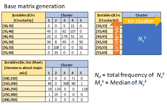
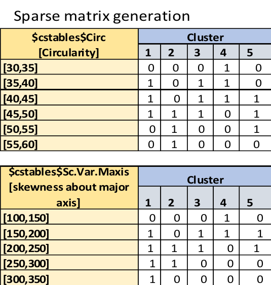
When we draw a cross-tab between unique interval of values of a variable and k number of clusters we expect, Nd to be fill the matrices in such a fashion that cross tab matrix $M_{v}^{k}$ has( $k$ = number of cluster , $v$ = the variable under consideration) only diagonal values. The maximum number of diagonal values possible is $max(l,k)$ [ $l$ = number of interval range considered for a variable, $k$ = number of clusters being evaluated]. Aiming to relax this segregation assumption (diagonal distribution of range vs cluster), we consider the values which are greater than $median(M_{v}^{k})$ of the frequency from the matrix generated as segregated values and take sum of such instances in $M_{v}^{k}$ .

The ratio of segregated instances by least possible instances gives us segregation factor. The reason for using $median(M_{v}^{k})$ and not any other measure is that, other measures are usually influenced by the range and mere occurrence of values in $M_{v}^{k}$ . Hence, median being the robust for the situation. The places where values are less than median can be used to identify observations which are having kind of outlier behaviour within the dataset. Following equation gives us the formula of getting segregated instances in $M_{v}^{k}$ .

Refer to caption — Figure 1: Crosstab Base Matrix for 2 variable examples

N_{v}^{k}=\displaystyle\sum_{x=1}^{l\ast k}\begin{cases}1&\text{ if }x>median(M_{v}^{k})\\ 0&\text{ if }x<=median(M_{v}^{k})\end{cases}

(2)

As for $explaination\ factor$ , $N_{d}$ observations has to be filled in $l\ast k$ places. The log ration of this defines how much of data can be eplained by this combination of clusters and variables.

Since unique values of varible is being used, in our experiments taking histogram of continuous varibles gave better results. Hence it is adviced to be use histogram bucketing for calculating cluster score for continuous variables.

Summation of $S_{v}^{k}$ for all variables gives us the score of cluster method on the data. As one can observe both parts of eqn. (1) are monotonous in nature hence the multiplication wil also lead to monotonous behaviour. This is can be well observed in experiments and results section.

4. Procedure

The $Algorithm1$ describes the procedure for calculating scores for the clusters

__________________________________________

Algorithm 1:: Cluster Score

__________________________________________

Data : $T_{d}$ is training data with $M$ variables and $N_{d}$ observtions,

Inputs: $k$ number of clusters

Output: $Cluster\ Score\ S^{k}$

Begin

for $v$ in $M$

if $v$ is Numeric

${v}^{\prime}=histogram(v)$ or $decile(v)$

$\mathbf{M_{v}^{k}}\ =$ Cross tab of $v^{\prime}$ with $k$ clusters

$\mathbf{N_{v}^{k}}:=$ Compute segregated instances using $M_{v}^{k}$ from Eqn. (2)

else if $v$ is Categorical / Ordinal

$\mathbf{M_{v}^{k}}\ =$ Cross tab of $v$ with $k$ clusters

$\mathbf{N_{v}^{k}}:=$ Compute segregated instances using $M_{v}^{k}$ from Eqn. (2)

end if;

$\mathbf{S_{v}^{k}}:=$ Compute cluster metric using $N_{v}^{k},\ l,\ k,\ N_{d}$ from Eqn. (1)

end;

$\mathbf{S^{k}}=\sum_{v=1}^{M}S_{v}^{k}$

End

__________________________________________

Since this method is non-parametric in nature, it is capable to understand the internal boundaries which are drawn from different cluster sizes and methods. Individual variable-cluster score Svk can be used to assess the quality of segregation made by cluster on that variable. Hence for drawing conclusion about clusters, one can almost always look for variables with low scores. Owing to this property this also helps in finding influential variables without using dependent / target variable.

This formulation adheres to all the points mentioned to be a “good” $metric$ , as explained below:

1)

The $metric$ calculation is invariant of datatype.
2)

Individual $S_{m}^{k}$ can be used to see which variable is being explained more than others for finding similarity.
3)

We can calculate same score for all variables that are not used for clustering and since this is not dependent on data, it is cross comparable.
4)

For the $metric$ , order dose not matter. Hence makes it viable even if the “name” of cluster changes.
5)

The $metric$ makes no assumption about underlying measures and hence, is invariant for different clustering methods.
6)

Owing to cross-tab behaviour the repeatability is assured, as the data is not going to change / or need to be re-calculated based on cluster method.

Also pertaining to business uses, practitioner can artificially weigh each variable to deduce the net score for clusters. These weights just need to be multiplied to individual scores to get the weighted scores. Number of bins / breaks in histogram for numeric variable can be kept constant or coarse bucketing can be used to bin each variable. In our experiment we observed, coarse buckets for individual variable yields better results.

One by product of this method is when $M_{v}^{k}$ calculated, clusters and observations with outlier behaviour can be extracted and its cross-feature influence can be estimated. This might be very helpful in analysis of fraud detection, anomaly detections and other rare event occurrence problems.

5. Experminetal Results

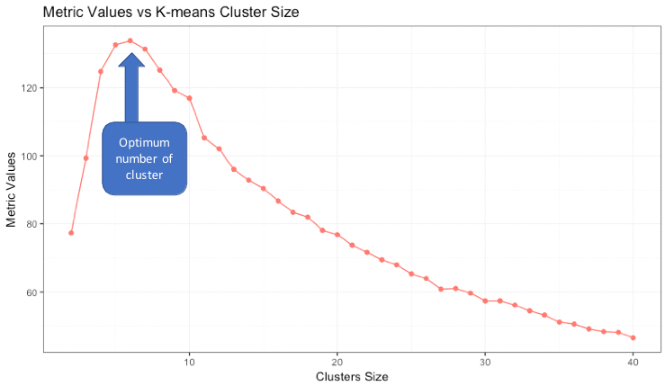
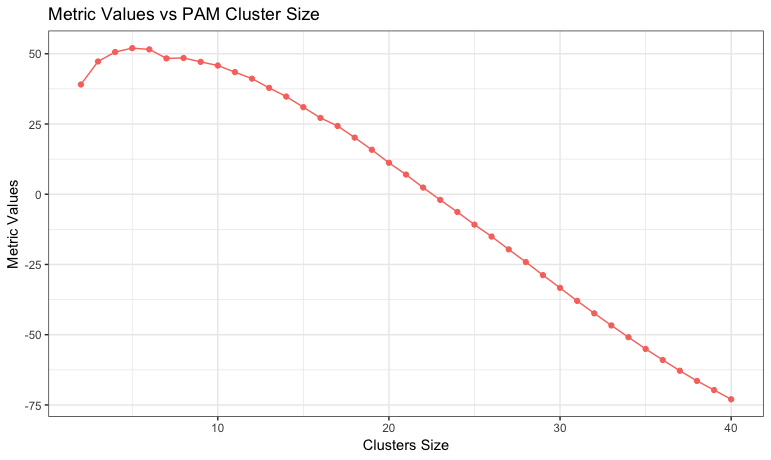
Showcased the capability of the metric with reference to understanding optimum number of cluster based on Vehicle Silhouettes data. We have run experiments with other datasets as well and the results are really encouraging and deterministic. If we look at Figure-3, for K-Means at close to 6 cluster our metric showcase highest seperation and high sparcity of results. Where as for PAM it comes to 5 Clusters as seen in Figure - 4.

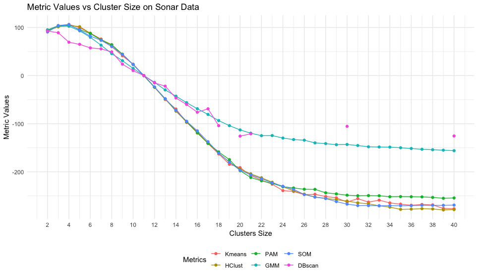
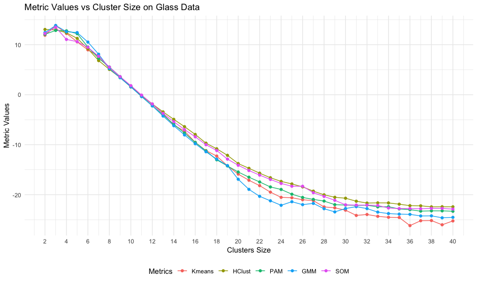
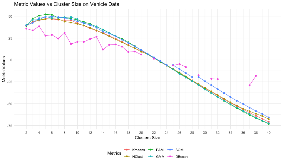
Figuer-5 showcase the evaluation comparison of different clustering techniques and how the metric value can help to compare them all with common reference point.

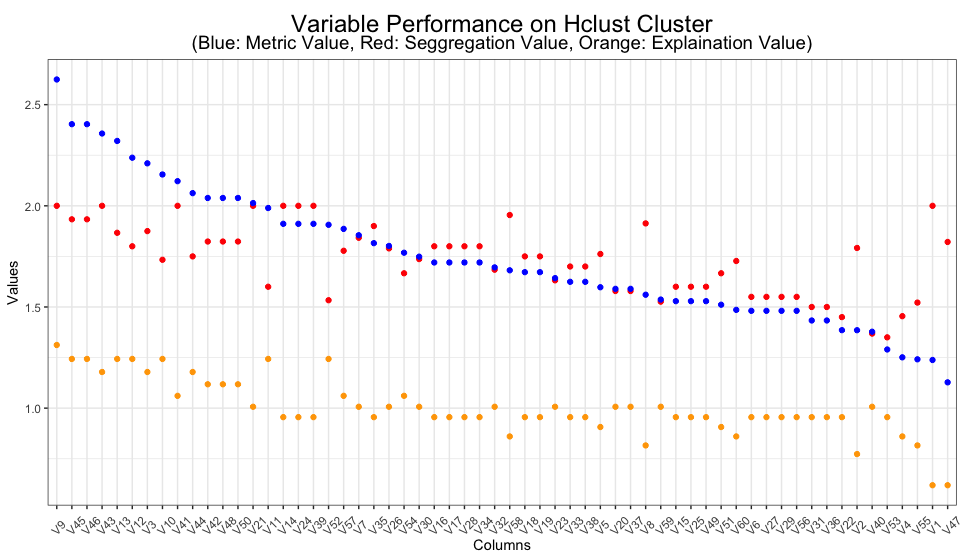
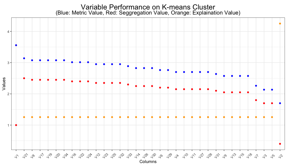
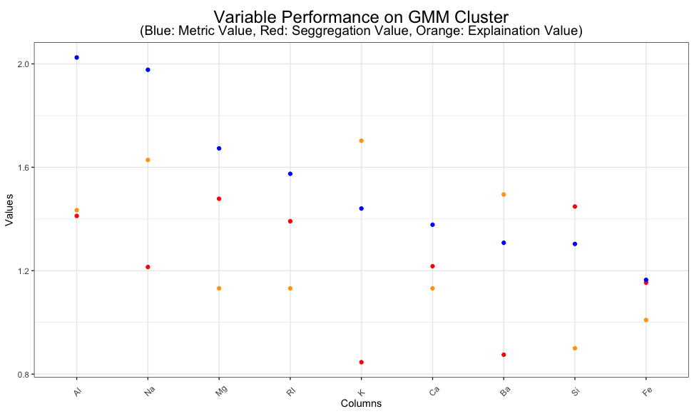
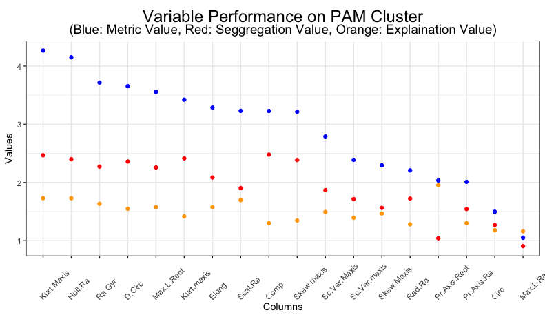
As mentioned earlier our metric also helps to find th right features for clustering. This is depicted on the Figure-6. Blue dots refers to the metric value, Orange indicates the explanation factor and Red dots represents the seggregation factors. This can help statistician to take informend decision on the cluster health and what all variables can be considered for clustering.

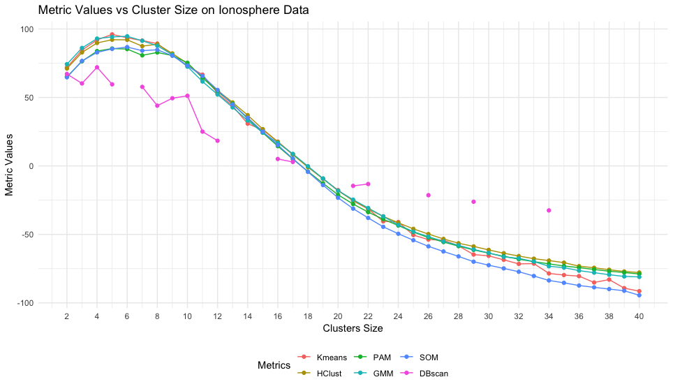
Further analysis on other data set are depeicted on Appendix-1.

6. Conclusion and Future Scope

In this paper we have proposed a new $metric$ to estimate the cluster behaviour from a non-parametric which is not based on any assumptions about clustering method. We also showed how this $metric$ can act as tools for the statisticians for making more sense from the data. The plots in our experiments not only helps in understand the cluster behaviour but can also be very insightful in rare event modelling.

There is a possibility to explore and extend this $metric$ in classification and value estimation modelling. If applied in such scenario, this can be implemented as loss function for linear and non-linear methods so that proper segmentation of data can be achieved.

References

Berkhin, Pavel. 2002. “Survey of Clustering Data Mining Techniques.”

H. Chouikhi, N. Ghazzali, M. Charrad. 2015. “A Comparison Study of Clustering Validity Indices.” Global Summit on Computer Information Technology (GSCIT) and IEEE, 1–4. https://doi.org/10.1109/GSCIT.2015.7353330.

H. Meroufel, N. Farhi, H. Mahi. 2017. “Comparative Study Between Validity Indices to Obtain the Optimal Cluster.” International Journal of Computer Electrical Engineering 9 (1): 1–8. https://doi.org/10.17706/ijcee.2017.9.1.343-350.

J. Hamalainen, T. Karkkainen, S. Jauhiainen. 2017. “Comparison of Internal Clustering Validation Indices for Prototype-Based Clustering.” MDPI Algorithms Articles, 1–14. https://doi.org/10.3390/a10030105.

M. K. Pakhira, U. Maulik, S. Bandyopadhyay. 2004. “Validity Index for Crisp and Fuzzy Clusters.” Pattern Recognition 37 (3): 487–501. https://doi.org/10.1016/j.patcog.2003.06.005.

O. Arbelaitz, J. Muguerza, I. Gurrutxaga. 2013. “An Extensive Comparative Study of Cluster Validity Indices.” Pattern Recognition 46 (1): 243–56. https://doi.org/10.1016/j.patcog.2012.07.021.

Xu, Rui, and D. Wunsch. 2005. “Survey of Clustering Algorithms.” IEEE Transactions on Neural Networks 16 (3): 645–78. https://doi.org/10.1109/TNN.2005.845141.

Unique Metric for Health Analysis with Optimization of Clustering Activity and Cross Comparison of Results from Different Approach

Abstract

Appendix A Appendix: Analysis on other Standard Data