Noisy Tug of War games for the $\mathbf{p}$-Laplacian: ${\mathbf{1<p<{\boldsymbol{\infty}}}}$

Abstract.

We propose a new finite difference approximation to the Dirichlet problem for the homogeneous $\mathbf{p}$-Laplace equation posed on an $N$-dimensional domain, in connection with the Tug of War games with noise. Our game and the related mean-value expansion that we develop, superposes the “deterministic averages” “$\frac{1}{2}(\inf+\sup)$” taken over balls, with the “stochastic averages” “$\fint$”, taken over $N$-dimensional ellipsoids whose aspect ratio depends on $N,\mathbf{p}$ and whose orientations span all directions while determining $\inf/\sup$. We show that the unique solutions $u_{\epsilon}$ of the related dynamic programming principle are automatically continuous for continuous boundary data, and coincide with the well-defined game values. Our game has thus the min-max property: the order of supremizing the outcomes over strategies of one player and infimizing over strategies of their opponent, is immaterial. We further show that domains satisfying the exterior corkscrew condition are game regular in this context, i.e. the family $\{u_{\epsilon}\}_{\epsilon\to 0}$ converges uniformly to the unique viscosity solution of the Dirichlet problem.

1. Introduction

In this paper, we study the finite difference approximations to the Dirichlet problem for the homogeneous $\mathrm{\bf p}$-Laplace equation $\Delta_{\mathrm{\bf p}}u=0$, posed on an $N$-dimensional domain, in connection to the dynamic programming principles of the so-called Tug of War games with noise.

It is a well known fact that for $u\in\mathcal{C}^{2}(\mathbb{R}^{N})$ there holds the following mean value expansion:

$$\fint_{B(x,r)}u(y)~{}\mbox{d}y=u(x)+\frac{r^{2}}{2(N+2)}\Delta u(x)+o(r^{2})\qquad\mbox{as }\;r\to 0+.$$

Indeed, an equivalent condition for harmonicity $\Delta u=0$ is the mean value property, and thus $\Delta u(x)$ provides the second-order offset from the satisfaction of this property. When we replace $B(x,r)$ by an ellipse $E(x,r;\alpha,\nu)=x+\{y\in\mathbb{R}^{N};~{}\langle y,\nu\rangle^{2}+\alpha^{2}|y-\langle y,\nu\rangle\nu|^{2}<\alpha^{2}r^{2}\}$ with the radius $r$, the aspect ratio $\alpha>0$ and oriented along some given unit vector $\nu$, we obtain:

$$\fint_{E(x,r;\alpha,\nu)}u(y)~{}\mbox{d}y=u(x)+\frac{r^{2}}{2(N+2)}\Big{(}\Delta u(x)+(\alpha^{2}-1)\langle\nabla^{2}u(x):\nu^{\otimes 2}\rangle\Big{)}+o(r^{2}).$$ (1.1)

Recalling the interpolation:

$$\Delta_{\mathrm{\bf p}}u=|\nabla u|^{\mathrm{\bf p}-2}\big{(}\Delta u+(\mathrm{\bf p}-2)\Delta_{\infty}u\big{)},$$ (1.2)

the formula (1.1) becomes: $\fint_{E(x,r;\alpha,\nu)}u(y)~{}\mbox{d}y=u(x)+\frac{r^{2}|\nabla u|^{2-\mathrm{\bf p}}}{2(N+2)}\Delta_{\mathrm{\bf p}}u(x)+o(r^{2}),$ for the choice $\alpha=\sqrt{\mathrm{\bf p}-1}$ and $\nu=\frac{\nabla u(x)}{|\nabla u(x)|}$. To obtain the mean value expansion where the left hand side averaging does not require the knowledge of $\nabla u(x)$ and allows for the identification of a $\mathrm{\bf p}$-harmonic function that is a priori only continuous, we need to, in a sense, additionally average over all equally probable vectors $\nu$. This can be carried out by superposing:

• the deterministic average “$\frac{1}{2}(\inf+\sup)$”, with

• the stochastic average “$\fint$”, taken over appropriate ellipses $E$ whose aspect ratio depends on $N,\mathrm{\bf p}$ and whose orientations $\nu$ span all directions while determining $\inf/\sup$ in (i).

In fact, such construction can be made precise (see Theorem 2.1), leading to the expansion:

$$\begin{split}\frac{1}{2}\Big{(}\inf_{z\in B(x,r)}+\sup_{z\in B(x,r)}\Big{)}&\fint_{\begin{minipage}{125.19194pt} $E\big{(}z,\gamma_{\mathrm{\bf p}}r,\alpha_{\mathrm{\bf p}}(\big{|}\frac{z-x}{r}\big{|}),\frac{z-x}{|z-x|}\big{)}$\end{minipage}}u(y)~{}\mbox{d}y\\ &\qquad\qquad\qquad\qquad=u(x)+\frac{\gamma_{\mathrm{\bf p}}^{2}r^{2}|\nabla u|^{\mathrm{\bf p}-2}}{2(N+2)}\Delta_{\mathrm{\bf p}}u(x)+o(r^{2}),\end{split}$$ (1.3)

with $\gamma_{\mathrm{\bf p}}$ that is a fixed stochastic sampling radius factor, and with $\alpha_{\mathrm{\bf p}}$ that is the aspect ratio in radial function of the deterministically chosen position $z\in B(x,r)$. The value of $\alpha_{\mathrm{\bf p}}$ varies quadratically from $1$ at the center of $B(x,r)$ to $a_{\mathrm{\bf p}}$ at its boundary, where $a_{\mathrm{\bf p}}$ and $\gamma_{\mathrm{\bf p}}$ satisfy the compatibility condition $\frac{N+2}{\gamma_{\mathrm{\bf p}}^{2}}+a_{\mathrm{\bf p}}^{2}=\mathrm{\bf p}-1$.

We will be concerned with the mean value expansions of the form (1.3), in connection with the specific Tug of War games with noise. This connection has been displayed in [11] by Peres and Scheffield, based on another interpolation property of $\Delta_{\mathrm{\bf p}}$:

$$\Delta_{\mathrm{\bf p}}u=|\nabla u|^{\mathrm{\bf p}-2}\Big{(}|\nabla u|\Delta_{1}u+(\mathrm{\bf p}-1)\Delta_{\infty}u\Big{)},$$ (1.4)

which has first appeared (in the context of the applications of $\Delta_{\mathrm{\bf p}}$ to image recognition) in [5]. Indeed, the construction in [11] interpolates from: (i) the $1$-Laplace operator $\Delta_{1}$ corresponding to the motion by curvature game studied by Kohn and Serfaty [6], to (ii) the $\infty$-Laplacian $\Delta_{\infty}$ corresponding to the pure Tug of War studied by Peres, Schramm, Scheffield and Wilson [10]. We remark that if one uses (1.2) instead of (1.4), one is lead to the games studied by Manfredi, Parviainen and Rossi [8], that interpolate from: $\Delta_{2}$ (classically corresponding [2] to Brownian motion), to $\Delta_{\infty}$; this approach however poses a limitation on the exponents $\mathrm{\bf p}\in[2,\infty)$.

The original game presented in [11] was a two-player, zero-sum game, stipulating that at each turn, position of the token is shifted by some vector $\sigma$ within the prescribed radius $r=\epsilon>0$, by a player who has won the coin toss, which is followed by a further update of the position by a random “noise vector”. The noise vector is uniformly distributed on the codimension-$2$ sphere, centered at the current position, contained within the hyperplane that is orthogonal to the last player’s move $\sigma$, and with radius proportional to $|\sigma|$ with factor $\gamma=\sqrt{\frac{N-1}{\mathrm{\bf p}-1}}$. We again interpret that $\gamma$ interpolates from: (i) $+\infty$ at the critical exponent $\mathrm{\bf p}=1$ that corresponds to choosing a direction line and subsequently determining its orientation, to (ii) $0$ at the critical exponent $\mathrm{\bf p}=\infty$ that corresponds to not adding the random noise at all.

In this paper we utilize the full $N$-dimensional sampling on ellipses $E$, rather than on spheres. Together with another modification taking into account the boundary data $F$, we achieve that the solutions of the dynamic programming principle at each scale $\epsilon>0$ are automatically continuous (in fact, they inherit the regularity of $F$) and coincide with the well-defined game values. The game stops almost surely under the additional compatibility condition, displayed in (4.2), on the scaling factors $\gamma_{\mathrm{\bf p}}$ and $a_{\mathrm{\bf p}}$ this condition is viable for any $\mathrm{\bf p}\in(1,\infty)$. Our game has then the min-max property: the order of supremizing the outcomes over strategies of one player and infimizing over strategies of his opponent, is immaterial.

This point has been left unanswered in the case of the game in [11], where the regularity (even measurability) of the possibly distinct game values was not clear. We also point out that in [1], the authors presented a variant of the [11] game where the deterministic / stochastic sampling takes place, respectively on: $(N-1)$-dimensional spheres, and $(N-1)$-dimensional balls within the orthogonal hyperplanes. They obtain the min-max property and continuity of solutions to the mean value expansion in their setting, albeit at the expense of much more complicated analysis, passing through measurable construction and comparison to game values. In our case the uniqueness and continuity follow directly, much like in the linear $\mathrm{\bf p}=2$ case where the $N$-dimensional averaging guarantees smoothness of harmonic functions.

1.1. The content and structure of the paper

In section 2, Theorem 2.1, we prove the validity of our main mean value expansion (1.3). In the following remarks we show how other expansions (with a wider range of exponents, with sampling set degenerating at the boundary, or pertaining to the [11] codimension-$2$ sampling) arise in the same analytical context.

In Theorem 3.1 in section 3, we obtain the existence, uniqueness and regularity of solutions $u_{\epsilon}$ to the dynamic programming principle (3.1) at each sampling scale $\epsilon$, that can be seen as a finite difference approximation to the $\mathrm{\bf p}$-Laplace Dirichlet problem with continuous boundary data $F$. In particular, each $u_{\epsilon}$ is continuous up to the boundary, where it assumes the values of $F$. Then, in Theorem 3.4 we show that in case $F$ is already a restriction of a $\mathrm{\bf p}$-harmonic function with non-vanishing gradient, the corresponding family $\{u_{\epsilon}\}_{\epsilon\to 0}$ uniformly converges to $F$ at the rate that is of first order in $\epsilon$. Our proof uses an analytical argument and it is based on the observation that for $s$ sufficiently large, the mapping $x\mapsto|x|^{s}$ yields the variation that pushes the $\mathrm{\bf p}$-harmonic function $F$ into the region of $\mathrm{\bf p}$-subharmonicity. In the linear case $\mathrm{\bf p}=2$, the quadratic correction $s=2$ suffices, otherwise we give a lower bound (3.8) for the admissible exponents $s=s(\mathrm{\bf p},N,F)$.

In section 4, we develop the probability setting for the Tug of War game modelled on (1.3) and (3.1). In Lemma 4.1 we show that the game stops almost surely if the scaling factors $\gamma_{\mathrm{\bf p}},a_{\mathrm{\bf p}}$ are chosen appropriately. Then in Theorem 4.2, using a classical martingale argument, we prove that our game has a value, coinciding with the unique, continuous solution $u_{\epsilon}$.

In section 5 we address convergence of the family $\{u_{\epsilon}\}_{\epsilon\to 0}$. In view of its equiboundedness, it suffices to prove equicontinuity. We first observe, in Theorem 5.1, that this property is equivalent to the seemingly weaker property of equicontinuity at the boundary. Again, our argument is analytical rather than probabilistic, based on the translation and well-posedness of (3.1). We then define the game regularity of the boundary points, which turns out to be a notion equivalent to the aforementioned boundary equicontinuity. Definition 5.2, Lemma 5.4 and Theorem 5.5 mimic the parallel statements in [11]. We further prove in Theorem 7.2 that any limit of a converging sequence in $\{u_{\epsilon}\}_{\epsilon\to 0}$ must be the viscosity solution to the $\mathrm{\bf p}$-harmonic equation with boundary data $F$. By uniqueness of such solutions, we obtain the uniform convergence of the entire family $\{u_{\epsilon}\}_{\epsilon\to 0}$ in case of the game regular boundary.

In section 6 we show that domains that satisfy the exterior corkscrew condition are game regular. The proof in Theorem 6.2 is based on the concatenating strategies technique and the annulus walk estimate taken from [11]. We expand the proofs and carefully provide the details omitted in [11], for the benefit of the reader less familiar with the probability techniques.

Finally, let us mention that similar results and approximations, together with their game-theoretical interpretation, can be also developed in other contexts, such as: the obstacle problems, nonlinear potential theory in Heisenberg group (or in other subriemannian geometries), Tug of War on graphs, the non-homogeneous problems, problems with non-constant coefficient $\mathrm{\bf p}$, and the fully nonlinear case of $\Delta_{\infty}$.

1.2. Notation for the $\mathrm{\bf p}$-Laplacian

Let $\mathcal{D}\subset\mathbb{R}^{N}$ be an open, bounded, connected set. Given $\mathrm{\bf p}\in(1,\infty)$, consider the following Dirichlet integral:

$$\mathcal{I}_{\mathrm{\bf p}}(u)=\int_{\mathcal{D}}|\nabla u(x)|^{\mathrm{\bf p}}~{}~{}\mbox{d}x\qquad\mbox{for all }~{}u\in W^{1,\mathrm{\bf p}}(\mathcal{D}),$$

that we want to minimize among all functions $u$ subject to some given boundary data. The condition for the vanishing of the first variation of $\mathcal{I}_{\mathrm{\bf p}}$, assuming sufficient regularity of $u$ so that the divergence theorem may be used, takes the form:

$$\int_{\mathcal{D}}\eta\,\mathrm{div}\big{(}|\nabla u|^{\mathrm{\bf p}-2}\nabla u\big{)}~{}\mbox{d}x=0\qquad\mbox{for all }\eta\in\mathcal{C}_{c}^{\infty}(\mathcal{D}),$$

which, by the fundamental theorem of Calculus of Variations, yields:

$$\Delta_{\mathrm{\bf p}}u=\mathrm{div}\Big{(}|\nabla u|^{\mathrm{\bf p}-2}\nabla u\Big{)}=0\quad\mbox{in }\mathcal{D}.$$ (1.5)

The operator in (1.5) is called the $\mathrm{\bf p}$-Laplacian, the partial differential equation (1.5) is called the $\mathrm{\bf p}$-harmonic equation and its solution $u$ is a $\mathrm{\bf p}$-harmonic function. It is not hard to compute:

$$\begin{split}\Delta_{\mathrm{\bf p}}u&=|\nabla u|^{\mathrm{\bf p}-2}\Delta u+\left\langle\nabla\big{(}|\nabla u|^{\mathrm{\bf p}-2}\big{)},\nabla u\right\rangle=|\nabla u|^{\mathrm{\bf p}-2}\Big{(}\Delta u+(\mathrm{\bf p}-2)\Big{\langle}\nabla^{2}u:\Big{(}\frac{\nabla u}{|\nabla u|}\Big{)}^{\otimes 2}\Big{\rangle}\Big{)},\end{split}$$

which is precisely (1.2). The second term in parentheses is called the $\infty$-Laplacian:

$$\Delta_{\infty}u=\Big{\langle}\nabla^{2}u:\Big{(}\frac{\nabla u}{|\nabla u|}\Big{)}^{\otimes 2}\Big{\rangle}.$$

The notation above refers to taking the scalar (Frobenius) product of the $N\times N$ matrix $\nabla^{2}u$ with the rank-1 matrix: $\big{(}\frac{\nabla u}{|\nabla u|}\big{)}^{\otimes 2}=\frac{\nabla u}{|\nabla u|}\otimes\frac{\nabla u}{|\nabla u|}=\big{(}\frac{\nabla u}{|\nabla u|}\big{)}\big{(}\frac{\nabla u}{|\nabla u|}\big{)}^{T}$. Using the scalar product of vectors notation, this is equivalent to writing: $\Delta_{\infty}u=\big{\langle}\nabla^{2}u\frac{\nabla u}{|\nabla u|},\frac{\nabla u}{|\nabla u|}\big{\rangle}$.

Applying (1.2) to the effect that $\Delta_{1}u=|\nabla u|^{-1}\big{(}\Delta u-\Delta_{\infty}u\big{)}$ and introducing it in (1.2) again, yields (1.4). Likewise, for every $1<\mathrm{\bf p}<\mathrm{\bf q}<\mathrm{\bf s}<\infty$ there holds:

$$(\mathrm{\bf s}-\mathrm{\bf q})|\nabla u|^{2-\mathrm{\bf p}}\Delta_{\mathrm{\bf p}}u=(\mathrm{\bf s}-\mathrm{\bf p})|\nabla u|^{2-\mathrm{\bf q}}\Delta_{\mathrm{\bf q}}u+(\mathrm{\bf p}-\mathrm{\bf q})|\nabla u|^{2-\mathrm{\bf s}}\Delta_{\mathrm{\bf s}}u.$$

1.3. Acknowledgments

The author is grateful to Yuval Peres for discussions about Tug of War games. Support by the NSF grant DMS-1613153 is acknowledged.

2. A mean value expansion for $\Delta_{\mathrm{\bf p}}$

For $\rho,\alpha>0$ and a unit vector $\nu\in\mathbb{R}^{N}$, we denote by $E(0,\rho;\alpha,\nu)$ the ellipse centered at $0$, with radius $\rho$, and with aspect ratio $\alpha$ oriented along $\nu$, namely:

$$E(0,\rho;\alpha,\nu)=\big{\{}y\in\mathbb{R}^{N};~{}\frac{\langle y,\nu\rangle^{2}}{\alpha^{2}}+|y-\langle y,\nu\rangle\nu|^{2}<\rho^{2}\big{\}}.$$

For $x\in\mathbb{R}^{N}$, we have the translated ellipse:

$$E(x,\rho;\alpha,\nu)=x+E(0,\rho;\alpha,\nu).$$

Note that, when $\nu=0$, this formula also makes sense and returns the ball $E(x,\rho;\alpha,0)=B(x,\rho)$ centered at $x$ and with radius $\rho$.

Given a continuous function $u:\mathbb{R}^{N}\to\mathbb{R}$, define the averaging operator:

$$\begin{split}\mathcal{A}\big{(}u;\rho,\alpha,\nu\big{)}(x)&=\fint_{E(x,\rho;\alpha,\nu)}u(y)~{}\mbox{d}y=\fint_{B(0,1)}u\big{(}x+\rho y+\rho(\alpha-1)\langle y,\nu\rangle\nu\big{)}~{}\mbox{d}y.\end{split}$$

In what follows, we will often use the above linear change of variables:

$$B(0,1)\ni y\mapsto\rho\alpha\langle y,\nu\rangle\nu+\rho\big{(}y-\langle y,\nu\rangle\nu\big{)}\in E(0,\rho;\alpha,\nu).$$

Theorem 2.1.

Given $\mathrm{\bf p}\in(1,\infty)$, fix any pair of scaling factors $\gamma_{\mathrm{\bf p}},a_{\mathrm{\bf p}}>0$ such that:

$$\frac{N+2}{\gamma_{\mathrm{\bf p}}^{2}}+a_{\mathrm{\bf p}}^{2}=\mathrm{\bf p}-1.$$ (2.1)

Let $u\in\mathcal{C}^{2}(\mathbb{R}^{N})$. Then, for every $x_{0}\in\mathbb{R}^{N}$ such that $\nabla u(x_{0})\neq 0$, we have:

$$\begin{split}\frac{1}{2}\Big{(}\inf_{x\in B(x_{0},r)}+&\sup_{x\in B(x_{0},r)}\Big{)}\mathcal{A}\Big{(}u;\gamma_{\mathrm{\bf p}}r,1+(a_{\mathrm{\bf p}}-1)\frac{|x-x_{0}|^{2}}{r^{2}},\frac{x-x_{0}}{|x-x_{0}|}\Big{)}(x)\\ &\quad=u(x_{0})+\frac{\gamma_{\mathrm{\bf p}}^{2}r^{2}}{2(N+2)}|\nabla u(x_{0})|^{2-\mathrm{\bf p}}\Delta_{\mathrm{\bf p}}u(x_{0})+o(r^{2})\qquad\mbox{ as }\;r\to 0+.\end{split}$$ (2.2)

The coefficient in the rate of convergence $o(r^{2})$ depends only on $\mathrm{\bf p}$, $N$, $\gamma_{\mathrm{\bf p}}$ and (in increasing manner) on $|\nabla u(x_{0})|$, $|\nabla^{2}u(x_{0})|$ and the modulus of continuity of $\nabla^{2}u$ at $x_{0}$.

The expression in the left hand side of the formula (2.2) should be understood as the deterministic average $\frac{1}{2}(\inf+\sup)$, on the ball $B(x_{0},r)$, of the function $x\mapsto f_{u}(x;x_{0},r)$ in:

$$\begin{split}f_{u}(x;x_{0},r)&=\mathcal{A}\Big{(}u;\gamma r,1+(a-1)\frac{|x-x_{0}|^{2}}{r^{2}},\frac{x-x_{0}}{|x-x_{0}|}\Big{)}(x)\\ &=\fint_{B(0,1)}u\big{(}x+\gamma ry+\frac{\gamma(a-1)}{r}\langle y,x-x_{0}\rangle(x-x_{0})\big{)}~{}\mbox{d}y,\end{split}$$ (2.3)

where $\gamma=\gamma_{\mathrm{\bf p}}$ and $a=a_{\mathrm{\bf p}}$. We will frequently use the notation:

$$S_{r}u(x_{0})=\frac{1}{2}\Big{(}\inf_{x\in B(x_{0},r)}+\sup_{x\in B(x_{0},r)}\Big{)}f_{u}(x;x_{0},r).$$ (2.4)

For each $x\in B(x_{0},r)$ the integral quantity in (2.3) returns the average of $u$ on the $N$-dimensional ellipse centered at $x$, with radius $\gamma r$, and with aspect ratio $\frac{r^{2}+(a-1)|x-x_{0}|^{2}}{r^{2}}$ along the orientation vector $\frac{x-x_{0}}{|x-x_{0}|}$. Equivalently, writing $x=x_{0}+ry$, the value $f_{u}(x;x_{0},r)$ is the average of $u$ on the scaled ellipse $x_{0}+rE\big{(}y,\gamma;1+(a-1)|y|^{2},\frac{y}{|y|}\big{)}$. Since the aspect ratio changes smoothly from $1$ to $a$ as $|x-x_{0}|$ decreases from $0$ to $r$, the said ellipse coincides with the ball $B(x_{0},\gamma r)$ at $x=x_{0}$ and it interpolates as $|x-x_{0}|\to r-$, to $E\big{(}x,\gamma r;a,\frac{x-x_{0}}{|x-x_{0}|}\big{)}.$

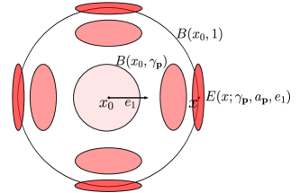
Figure 1. The sampling ellipses in the expansion (2.2), when $r=1$.

Proof of Theorem 2.1.

1. We fix $\gamma,a>0$ and consider the Taylor expansion of $u$ at a given $x\in B(x_{0},\rho)$ under the second integral in (2.3). Observe that the first order increments are linear in $y$, hence they integrate to $0$ on $B(0,1)$. These increments are of order $r$ and we get:

$$\begin{split}&f_{u}(x;~{}x_{0},r)\\ &=u(x)+\frac{1}{2}\Big{\langle}\nabla^{2}u(x):\fint_{B(0,1)}\Big{(}\gamma ry+\frac{\gamma(a-1)}{r}\langle y,x-x_{0}\rangle(x-x_{0})\Big{)}^{\otimes 2}~{}\mbox{d}y\Big{\rangle}+o(r^{2})\\ &=u(x)+\frac{\gamma^{2}}{2}\Big{\langle}\nabla^{2}u(x):r^{2}\fint_{B(0,1)}y^{\otimes 2}~{}\mbox{d}y+2(a-1)\fint_{B(0,1)}\langle y,x-x_{0}\rangle y~{}\mbox{d}y\otimes(x-x_{0})\\ &\qquad\qquad\qquad\qquad\qquad+\frac{(a-1)^{2}}{r^{2}}\Big{(}\fint_{B(0,1)}\langle y,x-x_{0}\rangle^{2}~{}\mbox{d}y\Big{)}(x-x_{0})^{\otimes 2}\Big{\rangle}+o(r^{2}).\end{split}$$ (2.5)

Recall now that:

$$\fint_{B(0,1)}y^{\otimes 2}~{}\mbox{d}y=\Big{(}\fint_{B(0,1)}y_{1}^{2}~{}\mbox{d}y\Big{)}Id_{N}=\frac{1}{N+2}Id_{N}.$$

Consequently, (2.5) becomes:

$$\begin{split}f_{u}(x;x_{0},r)&=u(x)+\frac{\gamma^{2}r^{2}}{2(N+2)}\Delta u(x)\\ &\quad+\frac{\gamma^{2}(a-1)}{2}\Big{(}\frac{2}{N+2}+\frac{(a-1)|x-x_{0}|^{2}}{r^{2}(N+2)}\Big{)}\big{\langle}\nabla^{2}u(x):(x-x_{0})^{\otimes 2}\big{\rangle}+o(r^{2})\\ &=\bar{f}_{u}(x;x_{0},r)+o(r^{2}),\end{split}$$

where a further Taylor expansion of $u$ at $x_{0}$ gives:

$$\begin{split}\bar{f}_{u}(x;x_{0},r)=u(x_{0})&+\langle\nabla u(x_{0}),x-x_{0}\rangle+\frac{\gamma^{2}r^{2}}{2(N+2)}\Delta u(x_{0})\\ &+\Big{(}\frac{1}{2}+\frac{\gamma^{2}(a-1)}{2}\Big{(}\frac{2}{N+2}+\frac{(a-1)|x-x_{0}|^{2}}{r^{2}(N+2)}\Big{)}\Big{)}\big{\langle}\nabla^{2}u(x_{0}):(x-x_{0})^{\otimes 2}\big{\rangle}.\end{split}$$

The left hand side of (2.2) thus satisfies:

$$\begin{split}\frac{1}{2}\Big{(}\inf_{x\in B(x_{0},r)}&f_{u}(x;x_{0},r)+\sup_{x\in B(x_{0},r)}f_{u}(x;x_{0},r)\Big{)}\\ &=\frac{1}{2}\Big{(}\inf_{x\in B(x_{0},r)}\bar{f}_{u}(x;x_{0},r)+\sup_{x\in B(x_{0},r)}\bar{f}_{u}(x;x_{0},r)\Big{)}+o(r^{2}),\end{split}$$ (2.6)

Since on $B(x_{0},r)$ we have: $\bar{f}_{u}(x;x_{0},r)=u(x_{0})+\langle\nabla u(x_{0}),x-x_{0}\rangle+O(r^{2})$, the assumption $\nabla u(x_{0})\neq 0$ implies that the continuous function $\bar{f}_{u}(\cdot\;;x_{0},r)$ attains its extrema on the boundary $\partial B(x_{0},r)$, provided that $r$ is sufficiently small. This reasoning justifies that $\bar{f}_{u}$ in (2.6) may be replaced by the quadratic polynomial function:

$$\begin{split}\bar{\bar{f}}_{u}(x;x_{0},r)=u(x_{0})&+\frac{\gamma^{2}r^{2}}{2(N+2)}\Delta u(x_{0})+\langle\nabla u(x_{0}),x-x_{0}\rangle\\ &+\Big{(}\frac{1}{2}+\frac{\gamma^{2}(a^{2}-1)}{2(N+2)}\Big{)}\big{\langle}\nabla^{2}u(x_{0}):(x-x_{0})^{\otimes 2}\big{\rangle}.\end{split}$$

2. We now argue that $\bar{\bar{f}}_{u}$ attains its extrema on $\bar{B}(x_{0},r)$, up to error $O(r^{3})$ whenever $r$ is sufficiently small, precisely at the opposite boundary points $x_{0}+r\frac{\nabla u(x_{0})}{|\nabla u(x_{0})|}$ and $x_{0}-r\frac{\nabla u(x_{0})}{|\nabla u(x_{0})|}$. We recall the adequate argument from [11], for the convenience of the reader. After translating and rescaling, it suffices to investigate the extrema on $\bar{B}(0,1)$, of the functions:

$$g_{r}(x)=\langle a,x\rangle+r\langle A:x^{\otimes 2}\rangle,$$

where $a\in\mathbb{R}^{N}$ is of unit length and $A\in\mathbb{R}^{N\times N}_{\mathrm{sym}}$. Fix a small $r>0$ and let $x_{max}\in\partial B(0,1)$ be a maximizer of $g_{r}$. Writing $g_{r}(x_{max})\geq g_{r}(a)$, we obtain:

$$\begin{split}\langle a,x_{max}\rangle&\geq 1+r\big{\langle}A:a^{\otimes 2}-x_{max}^{\otimes 2}\big{\rangle}\\ &\geq 1-r|A|\big{|}a^{\otimes 2}-x_{max}^{\otimes 2}\big{|}\geq 1-2r|A||a-x_{max}|.\end{split}$$

Thus there holds: $|a-x_{max}|^{2}=2-2\langle a,x_{max}\rangle\leq 4r|A||a-x_{max}|$, and so finally:

$$|a-x_{max}|\leq 4r|A|.$$

Since $\langle a,x_{max}\rangle\leq 1$, we conclude that:

$$\begin{split}0\leq g_{r}(x_{max})-g_{r}(a)&=\langle a,x_{max}-a\rangle+r\big{\langle}A:x_{max}^{\otimes 2}-a^{\otimes 2}\big{\rangle}\\ &\leq r\big{\langle}A:x_{max}^{\otimes 2}-a^{\otimes 2}\big{\rangle}\leq 2r|A||a-x_{max}|\leq 8r^{2}|A|^{2}.\end{split}$$

Likewise, for a minimizer $x_{min}$ we have: $0\geq g_{r}(x_{min})-g_{r}(-a)\geq-8r^{2}|A|^{2}$. It follows that:

$$\begin{split}\big{|}\frac{1}{2}\big{(}g_{r}(x_{min})+&g_{r}(x_{max})\big{)}-\frac{1}{2}\big{(}g_{r}(-a)+g_{r}(a)\big{)}\big{|}\leq 8r^{2}|A|^{2},\end{split}$$

which proves the claim for the unscaled functions $\bar{\bar{f}}_{u}$.

3. We now observe that for $\gamma=\gamma_{\mathrm{\bf p}}$, $a=a_{\mathrm{\bf p}}$ satisfying (2.1), there holds:

$$\begin{split}\frac{1}{2}\Big{(}&\inf_{x\in B(x_{0},r)}\bar{\bar{f}}_{u}(x;x_{0},r)+\sup_{x\in B(x_{0},r)}\bar{\bar{f}}_{u}(x;x_{0},r)\Big{)}\\ &=u(x_{0})+\frac{\gamma^{2}r^{2}}{2(N+2)}\Delta u(x_{0})+r^{2}\Big{(}\frac{1}{2}+\frac{\gamma^{2}(a^{2}-1)}{2(N+2)}\Big{)}\Delta_{\infty}u(x_{0})+O(r^{3})\\ &=u(x_{0})+\frac{\gamma^{2}r^{2}}{2(N+2)}\Big{(}\Delta u(x_{0})+\Big{(}\frac{N+2}{\gamma^{2}}+a^{2}-1\Big{)}\Delta_{\infty}u(x_{0})\Big{)}+O(r^{3})\\ &=u(x_{0})+\frac{\gamma_{\mathrm{\bf p}}^{2}r^{2}}{2(N+2)}\Big{(}\Delta u(x_{0})+(\mathrm{\bf p}-2)\Delta_{\infty}u(x_{0})\Big{)}+O(r^{3})\\ &=u(x_{0})+\gamma_{\mathrm{\bf p}}^{2}r^{2}\frac{|\nabla u(x_{0})|^{2-\mathrm{\bf p}}}{2(N+2)}\Delta_{\mathrm{\bf p}}u(x_{0})+O(r^{3}),\end{split}$$ (2.7)

where in the last step we used (1.2). This completes the proof in view of (2.6).   

Remark 2.2.

A few heuristic observations are in order. When $\mathrm{\bf p}\to\infty$, one can take $a_{\mathrm{\bf p}}=1$ and $\gamma_{\mathrm{\bf p}}\sim 0$ in (2.1), whereas (2.2) is linked to the following well-known expansion and to the absolutely minimizing Lipschitz extension property of the infinitely harmonic functions:

$$\frac{1}{2}\Big{(}\inf_{B(x_{0},r)}u+\sup_{B(x_{0},r)}u\Big{)}=u(x_{0})+\frac{r^{2}}{2}\Delta_{\infty}u(x_{0})+o(r^{2}).$$

When $\mathrm{\bf p}=2$, then choosing $a_{\mathrm{\bf p}}=1$ and $\gamma_{\mathrm{\bf p}}\sim\infty$ corresponds to taking both stochastic and deterministic averages on balls, whose radii have ratio $\sim\infty$. Equivalently, one may average stochastically on $B(x_{0},r)$ and deterministically on $B(x_{0},0)\sim\{x_{0}\}$, consistently with another familiar expansion:

$$\mathcal{A}\big{(}u;r,1,0\big{)}(x_{0})=\fint_{B(x_{0},r)}u(y)~{}\mbox{d}y=u(x_{0})+\frac{r^{2}}{2(N+2)}\Delta_{2}u(x_{0})+o(r^{2}).$$

On the other hand, when $\mathrm{\bf p}\to 1+$, then there must be $a_{\mathrm{\bf p}}\to 0+$ and the critical choice $a_{\mathrm{\bf p}}=0$ is the only one valid for every $\mathrm{\bf p}\in(1,\infty)$. It corresponds to varying the aspect ratio along the radius of $B(x_{0},r)$ from $1$ to $0$ rather than to $a_{\mathrm{\bf p}}>0$, and taking the stochastic averaging domains to be the corresponding ellipses:

$$E\big{(}x,\gamma r;1-\frac{|x-x_{0}|^{2}}{r^{2}},\frac{x-x_{0}}{|x-x_{0}|}\big{)},$$

whose radius $\gamma r$ is scaled by the factor $\gamma=\sqrt{\frac{N+2}{\mathrm{\bf p}-1}}$. At $x=x_{0}$, the ellipse above coincides with the ball $B(x_{0},\gamma r)$, whereas as $|x-x_{0}|\to r-$ it degenerates to the $(N-1)$-dimensional ball:

$$E\big{(}x,\gamma r;0,\frac{x-x_{0}}{|x-x_{0}|}\big{)}=x+\Big{\{}y\in\mathbb{R}^{N};~{}\langle y,x-x_{0}\rangle=0\mbox{ and }|y|<r\sqrt{\frac{N+2}{\mathrm{\bf p}-1}}\;\Big{\}}.$$

The resulting mean value expansion is then:

$$\begin{split}\frac{1}{2}\Big{(}\inf_{x\in B(x_{0},r)}+&\sup_{x\in B(x_{0},r)}\Big{)}\mathcal{A}\big{(}u;\gamma r,1-\frac{|x-x_{0}|^{2}}{r^{2}},\frac{x-x_{0}}{|x-x_{0}|}\big{)}(x)\\ &\quad=u(x_{0})+\frac{r^{2}}{2(\mathrm{\bf p}-1)}|\nabla u(x_{0})|^{2-\mathrm{\bf p}}\Delta_{\mathrm{\bf p}}u(x_{0})+o(r^{2}).\end{split}$$ (2.8)

Remark 2.3.

In [11], instead of averaging on an $N$-dimensional ellipse, the average is taken on the $(N-2)$-dimensional sphere centered at $x$, with some radius $\gamma|x-x_{0}|$, and contained within the hyperplane perpendicular to $x-x_{0}$. The radius of the sphere thus increases linearly from $0$ to $\gamma r$ with a factor $\gamma>0$, as $|x-x_{0}|$ varies from $0$ to $r$. This corresponds to evaluating on $B(x_{0},r)$ the deterministic averages of:

$$f_{u}(x;x_{0},r)=\fint_{\partial B^{N-1}(0,1)}u\big{(}x+\gamma|x-x_{0}|R(x)y\big{)}~{}\mbox{d}y.$$

Here, $R(x)\in SO(N)$ is such that $R(x)e_{N}=\frac{x-x_{0}}{|x-x_{0}|}$, and $\partial B^{N-1}(0,1)$ stands for the $(N-2)$-dimensional sphere of unit radius, viewed as a subset of $\mathbb{R}^{N}$ contained in the subspace $\mathbb{R}^{N-1}$ orthogonal to $e_{N}$. Note that $x\mapsto R(x)$ can be only locally defined as a $\mathcal{C}^{2}$ function. However, the argument as in the proof of Theorem 2.1, can still be applied to get:

$$\begin{split}f_{u}(x;x_{0},r)&=u(x)+\frac{1}{2}\Big{\langle}\nabla^{2}u(x):\gamma^{2}|x-x_{0}|^{2}\fint_{\partial B^{N-1}(0,1)}\big{(}R(x)y\big{)}^{\otimes 2}~{}\mbox{d}y\Big{\rangle}+o(r^{2})\\ &=u(x)+\frac{\gamma^{2}}{2(N-1)}\Big{(}|x-x_{0}|^{2}\Delta u(x)-\big{\langle}\nabla^{2}u(x):(x-x_{0})^{\otimes 2}\big{\rangle}\Big{)}+o(r^{2})\\ &=u(x_{0})+\langle\nabla u(x_{0}),x-x_{0}\rangle+\frac{\gamma^{2}}{2(N-1)}|x-x_{0}|^{2}\Delta u(x_{0})\\ &\qquad\quad\;\;\,+\Big{(}\frac{1}{2}-\frac{\gamma^{2}}{2(N-1)}\Big{)}\big{\langle}\nabla^{2}u(x_{0}):(x-x_{0})^{\otimes 2}\big{\rangle}+o(r^{2})\end{split}$$

where we used the general formula $\fint_{\partial B^{d}(0,1)}y^{\otimes 2}~{}\mbox{d}y=\frac{1}{d}\fint_{\partial B^{d}(0,1)}|y|^{2}~{}\mbox{d}yId_{d}=\frac{1}{d}Id_{d}$, so that:

$$\fint_{\partial B^{N-1}(0,1)}\big{(}R(x)y\big{)}^{\otimes 2}~{}\mbox{d}y=\frac{1}{N-1}R(x)\big{(}Id_{N}-e_{N}^{\otimes 2}\big{)}R(x)^{T}=\frac{1}{N-1}\Big{(}Id_{N}-\big{(}\frac{x-x_{0}}{|x-x_{0}|}\big{)}^{\otimes 2}\Big{)}.$$

Calling $\bar{\bar{f}}_{u}$ the polynomial:

$$\begin{split}\bar{\bar{f}}_{u}(x;x_{0},r)=&~{}u(x_{0})+\langle\nabla u(x_{0}),x-x_{0}\rangle\\ &+\Big{\langle}\frac{\gamma^{2}}{2(N-1)}\Delta u(x_{0})Id_{N}+\Big{(}\frac{1}{2}-\frac{\gamma^{2}}{2(N-1)}\Big{)}\nabla^{2}u(x_{0}):(x-x_{0})^{\otimes 2}\Big{\rangle},\end{split}$$

the claim in Step 2 of proof of Theorem 2.1 yields:

$$\begin{split}\frac{1}{2}\Big{(}&\inf_{x\in B(x_{0},r)}\bar{\bar{f}}_{u}(x;x_{0},r)+\sup_{x\in B(x_{0},r)}\bar{\bar{f}}_{u}(x;x_{0},r)\Big{)}\\ &=u(x_{0})+\frac{\gamma^{2}r^{2}}{2(N-1)}\Big{(}\Delta u(x_{0})+\Big{(}\frac{N-1}{\gamma^{2}}-1\Big{)}\Delta_{\infty}u(x_{0})\Big{)}+O(r^{3}).\end{split}$$

Clearly, there holds $\frac{N-1}{\gamma^{2}}-1=\mathrm{\bf p}-2$, precisely for the scaling factor $\gamma=\sqrt{\frac{N-1}{\mathrm{\bf p}-1}}$ as in [11]. In this case, we get the mean value expansion with the same coefficient as in (2.8):

$$\begin{split}\frac{1}{2}\Big{(}\inf_{x\in B(x_{0},r)}+&\sup_{x\in B(x_{0},r)}\Big{)}f_{u}(x;x_{0},r)\\ &\quad=u(x_{0})+\frac{r^{2}}{2(\mathrm{\bf p}-1)}|\nabla u(x_{0})|^{2-\mathrm{\bf p}}\Delta_{\mathrm{\bf p}}u(x_{0})+o(r^{2}).\end{split}$$ (2.9)

3. The dynamic programming principle and the first convergence theorem

Let $\mathcal{D}\subset\mathbb{R}^{N}$ be an open, bounded, connected domain and let $F\in\mathcal{C}(\mathbb{R}^{N})$ be a bounded data function. Given $\gamma_{\mathrm{\bf p}},a_{\mathrm{\bf p}}>0$ as in (2.1), recall the definition of $S_{r}$ in (2.4). We then have:

Theorem 3.1.

For every $\epsilon\in(0,1)$ there exists a unique Borel, bounded function $u:\mathbb{R}^{N}\to\mathbb{R}$ (denoted further by $u_{\epsilon}$), automatically continuous, such that:

$$u(x)=d_{\epsilon}(x)S_{\epsilon}u(x)+\big{(}1-d_{\epsilon}(x)\big{)}F(x)\qquad\mbox{ for all }\;x\in\mathbb{R}^{N},$$ (3.1)

where the scaled distance function $d_{\epsilon}:\mathbb{R}^{N}\to[0,1]$ is given by:

$$d_{\epsilon}(x)=\frac{1}{\epsilon}\min\big{\{}\epsilon,\mathrm{dist}\big{(}x,\mathbb{R}^{N}\setminus\mathcal{D}\big{)}\big{\}}.$$

The solution operator to (3.1) is monotone, i.e. if $F\leq\bar{F}$ then the corresponding solutions satisfy: $u_{\epsilon}\leq\bar{u}_{\epsilon}$. Moreover $\|u\|_{\mathcal{C}(\mathbb{R}^{N})}\leq\|F\|_{\mathcal{C}(\mathbb{R}^{N})}$.

Proof.

1. The solution $u$ of (3.1) is a fixed point of the operator $T_{\epsilon}v=d_{\epsilon}S_{\epsilon}v+(1-d_{\epsilon})F$. Recall that:

$$\begin{split}&(S_{\epsilon}v)(x)=\frac{1}{2}\Big{(}\inf_{z\in B(0,1)}+\sup_{z\in B(0,1)}\Big{)}f_{v}(x+\epsilon z;x,\epsilon)\\ &\mbox{where: }\quad f_{v}(x+\epsilon z;x,\epsilon)=\fint_{x+\epsilon E(z,\gamma_{\mathrm{\bf p}};1+(a_{\mathrm{\bf p}}-1)|z|^{2},\frac{z}{|z|})}v(w)~{}\mbox{d}w.\end{split}$$ (3.2)

Observe that for a fixed $\epsilon$ and $x$, and given a bounded Borel function $v:\mathbb{R}^{N}\to\mathbb{R}$, the average $f_{v}$ is continuous in $z\in\bar{B}(0,1)$. In view of continuity of the weight $d_{\epsilon}$ and the data $F$, it is not hard to conclude that both $T_{\epsilon},S_{\epsilon}$ likewise return a bounded continuous function, so in particular the solution to (3.1) is automatically continuous. We further note that $S_{\epsilon}$ and $T_{\epsilon}$ are monotone, namely: $S_{\epsilon}v\leq S_{\epsilon}\bar{v}$ and $T_{\epsilon}v\leq T_{\epsilon}\bar{v}$ if $v\leq\bar{v}$.

The solution $u$ of (3.1) is obtained as the limit of iterations $u_{n+1}=T_{\epsilon}u_{n}$, where we set $u_{0}\equiv const\leq\inf F$. Since $u_{1}=T_{\epsilon}u_{0}\geq u_{0}$ on $\mathbb{R}^{N}$, by monotonicity of $T_{\epsilon}$, the sequence $\{u_{n}\}_{n=0}^{\infty}$ is nondecreasing. It is also bounded (by $\|F\|_{\mathcal{C}(\mathbb{R}^{N})}$) and thus it converges pointwise to a (bounded, Borel) limit $u:\mathbb{R}^{N}\to\mathbb{R}$. Observe now that:

$$\begin{split}|T_{\epsilon}u_{n}(x)&-T_{\epsilon}u(x)|\leq|S_{\epsilon}u_{n}(x)-S_{\epsilon}u(x)|\\ &\leq\sup_{z\in B(0,1)}\fint_{x+\epsilon E(z,\gamma_{\mathrm{\bf p}};1+(a_{\mathrm{\bf p}}-1)|z|^{2},\frac{z}{|z|})}|u_{n}-u|(w)~{}\mbox{d}w\leq C_{\epsilon}\int_{\mathcal{D}}|u_{n}-u|(w)~{}\mbox{d}w,\end{split}$$ (3.3)

where $C_{\epsilon}$ is the lower bound on the volume of the sampling ellipses. By the monotone convergence theorem, it follows that the right hand side in (3.3) converges to $0$ as $n\to\infty$. Consequently, $u=T_{\epsilon}u$, proving existence of solutions to (3.1).

2. We now show uniqueness. If $u,\bar{u}$ both solve (3.1), then define $M=\sup_{x\in\mathbb{R}^{N}}|u(x)-\bar{u}(x)|=\sup_{x\in\mathcal{D}}|u(x)-\bar{u}(x)|$ and consider any maximizer $x_{0}\in\mathcal{D}$, where $|u(x_{0})-\bar{u}(x_{0})|=M$. By the same bound in (3.3) it follows that:

$$M=|u(x_{0})-\bar{u}(x_{0})|=d_{\epsilon}(x_{0})|S_{\epsilon}u(x_{0})-S_{\epsilon}\bar{u}(x_{0})|\leq\sup_{z\in B(0,1)}f_{|u-\bar{u}|}(x+\epsilon z;x,\epsilon)\leq M,$$

yielding in particular $\fint_{B(x_{0},\gamma_{\mathrm{\bf p}}\epsilon)}|u-\bar{u}|(w)~{}\mbox{d}w=M$. Consequently, $B(x_{0},\gamma_{\mathrm{\bf p}}\epsilon)\subset D_{M}=\{|u-\bar{u}|=M\}$ and hence the set $D_{M}$ is open in $\mathbb{R}^{N}$. Since $D_{M}$ is obviously closed and nonempty, there must be $D_{M}=\mathbb{R}^{N}$ and since $u-\bar{u}=0$ on $\mathbb{R}^{N}\setminus\mathcal{D}$, it follows that $M=0$. Thus $u=\bar{u}$, proving the claim. Finally, we remark that the monotonicity of $S_{\epsilon}$ yields the monotonicity of the solution operator to (3.1).   

Remark 3.2.

It follows from (3.3) that the sequence $\{u_{n}\}_{n=1}^{\infty}$ in the proof of Theorem 3.1 converges to $u=u_{\epsilon}$ uniformly. In fact, the iteration procedure $u_{n+1}=Tu_{n}$ started by any bounded and continuous function $u_{0}$ converges uniformly to the uniquely given $u_{\epsilon}$. We further remark that if $F$ is Lipschitz continuous then $u_{\epsilon}$ is likewise Lipschitz, with Lipschitz constant depending (in nondecreasing manner) on the following quantities: $1/\epsilon$, $\|F\|_{\mathcal{C}(\partial\mathcal{D})}$ and the Lipschitz constant of $F_{\mid\partial\mathcal{D}}$.

Remark 3.3.

If we replace $d_{\epsilon}$ in Theorem 3.1 by the indicator function $\chi_{\mathcal{D}}$, the resulting solutions to (3.1) will in general be discontinuous, regardless of the regularity of $F$. The classical Ascoli-Arzelà theorem could not be thus used in this setting for the proof of convegence of $\{u_{\epsilon}\}_{\epsilon\to 0}$. It would still be possible, however, to obtain the asymptotic regularity and prove the uniform convergence (see section 5) by analyzing the dependence of variation of $u_{\epsilon}$ on $\epsilon$. Another possible interpolation weight in (3.1) is: $\tilde{d}_{\epsilon}(x)=\frac{1}{\epsilon}\min\big{\{}\epsilon,\mathrm{dist}\big{(}x,(\mathbb{R}^{N}\setminus\mathcal{D})+\bar{B}_{\epsilon}(0)\big{)}\big{\}}$, which varies from $0$ to $1$ on the $(\epsilon,2\epsilon)$ boundary layer, rather than the layer $(0,\epsilon)$. All results in this work remain valid with $\tilde{d}_{\epsilon}$, whereas the advantage of such a choice is that the resulting game stopping position always takes place in $\mathcal{D}$.

We prove the following first convergence result. Our argument will be analytical, although a probabilistic proof is possible as well, based on the interpretation of $u_{\epsilon}$ in Theorem 4.2.

Theorem 3.4.

Let $F\in\mathcal{C}^{2}(\mathbb{R}^{N})$ be a bounded data function that satisfies on some open set $U$, compactly containing $\mathcal{D}$:

$$\Delta_{\mathrm{\bf p}}F=0\quad\mbox{ and }\quad\nabla F\neq 0\qquad\mbox{in }\;U.$$ (3.4)

Then the solutions $u_{\epsilon}$ of (3.1) converge to $F$ uniformly in $\mathbb{R}^{N}$, namely:

$$\|u_{\epsilon}-F\|_{\mathcal{C}(\mathcal{D})}\leq C\epsilon\qquad\mbox{ as }\;\epsilon\to 0,$$ (3.5)

with a constant $C$ depending on $F$, $U$, $\mathcal{D}$ and $\mathrm{\bf p}$, but not on $\epsilon$.

Proof.

1. We first note that since $u_{\epsilon}=F$ on $\mathbb{R}^{N}\setminus\mathcal{D}$ by construction, (3.5) indeed implies the uniform convergence of $u_{\epsilon}$ in $\mathbb{R}^{N}$. Also, by translating $\mathcal{D}$ if necessary, we may without loss of generality assume that $B(0,1)\cap U=\emptyset$.

We now show that there exists $s\geq 2$ and $\hat{\epsilon}>0$ such that the following functions:

$$v_{\epsilon}(x)=F(x)+\epsilon|x|^{s}$$

satisfy, for every $\epsilon\in(0,\hat{\epsilon})$:

$$\nabla v_{\epsilon}\neq 0\quad\mbox{ and }\quad\Delta_{\mathrm{\bf p}}v_{\epsilon}\geq\epsilon s\cdot|\nabla{v_{\epsilon}}|^{{\mathrm{\bf p}}-2}\quad\mbox{ in }\;\bar{\mathcal{D}}.$$ (3.6)

Observe first the following direct formulas:

$$\begin{split}&\nabla|x|^{s}=s|x|^{s-2}x,\qquad\nabla^{2}|x|^{s}=s(s-2)|x|^{s-4}x^{\otimes 2}+s|x|^{s-2}Id_{N},\\ &\Delta|x|^{s}=s(s-2+N)|x|^{s-2}.\end{split}$$

Fix $x\in\bar{\mathcal{D}}$ and denote $a=\nabla v_{\epsilon}(x)$ and $b=\nabla F(x)$. Then, by (3.4) we have:

$$\begin{split}\Delta_{\mathrm{\bf p}}v_{\epsilon}(x)&=|\nabla v_{\epsilon}(x)|^{\mathrm{\bf p}-2}\Bigg{(}\epsilon\Delta|x|^{s}+(\mathrm{\bf p}-2)\epsilon\Big{\langle}\nabla^{2}|x|^{s}:\big{(}\frac{a}{|a|}\big{)}^{\otimes 2}\Big{\rangle}\\ &\qquad\qquad\qquad\qquad\qquad+(\mathrm{\bf p}-2)\Big{\langle}\nabla^{2}F(x):\big{(}\frac{a}{|a|}\big{)}^{\otimes 2}-\big{(}\frac{b}{|b|}\big{)}^{\otimes 2}\Big{\rangle}\Bigg{)}\\ &\geq|\nabla v_{\epsilon}(x)|^{\mathrm{\bf p}-2}\epsilon s|x|^{s-2}\Bigg{(}s-2+N+(\mathrm{\bf p}-2)\Big{(}1-\frac{4|\nabla^{2}F(x)|}{|\nabla F(x)|}|x|\Big{)}\Bigg{)}.\end{split}$$ (3.7)

Above, we have also used the bound:

$$\Big{\langle}\nabla^{2}|x|^{s}:\big{(}\frac{a}{|a|}\big{)}^{\otimes 2}\Big{\rangle}=s(s-2)|x|^{s-2}\Big{\langle}\frac{a}{|a|},\frac{x}{|x|}\Big{\rangle}^{2}+s|x|^{s-2}\geq s|x|^{s-2},$$

together with the straightforward estimate: $\big{|}\big{(}\frac{a}{|a|}\big{)}^{\otimes 2}-\big{(}\frac{b}{|b|}\big{)}^{\otimes 2}\big{|}\leq 4\frac{|a-b|}{|b|}.$ The claim (3.6) hence follows by fixing a large exponent $s$ that satisfies:

$${s\geq 3-N+|\mathrm{\bf p}-2|\cdot\max_{y\in\bar{\mathcal{D}}}\Big{\{}4|y|\frac{|\nabla^{2}F(y)|}{|\nabla F(y)|}}\Big{\}},$$ (3.8)

so that the quantity in the last line parentheses in (3.7) is greater than $1$, and further taking $\epsilon>0$ small enough to have: $\min_{\bar{\mathcal{D}}}|\nabla v_{\epsilon}|>0$.

2. We claim that $s$ and $\hat{\epsilon}$ in step 1 can further be chosen in a way that for all $\epsilon\in(0,\hat{\epsilon})$:

$$v_{\epsilon}\leq S_{\epsilon}v_{\epsilon}\quad\text{in}\,\,\bar{\mathcal{D}}.$$ (3.9)

Indeed, a careful analysis of the remainder terms in the expansion (2.2) reveals that:

$$v_{\epsilon}(x)-S_{\epsilon}v_{\epsilon}(x)=-\frac{\epsilon^{2}}{\mathrm{\bf p}-1}|\nabla{v}_{\epsilon}(x)|^{2-\mathrm{\bf p}}\Delta_{\mathrm{\bf p}}v_{\epsilon}(x)+R_{2}(\epsilon,s),$$ (3.10)

where:

$$|R_{2}(\epsilon,s)|\leq C_{\mathrm{\bf p}}\epsilon^{2}\displaystyle{\mbox{osc}_{B(x,(1+\gamma_{p})\epsilon)}}|\nabla^{2}v_{\epsilon}|+C\epsilon^{3}.$$

Above, we denoted by $C_{\mathrm{\bf p}}$ a constant depending only on $\mathrm{\bf p}$, whereas $C$ is a constant depending only $|\nabla{v_{\epsilon}}|$ and $|\nabla^{2}v_{\epsilon}|$, that remain uniformly bounded for small $\epsilon$. Since $v_{\epsilon}$ is the sum of the smooth on $U$ function $x\mapsto\epsilon|x|^{s}$, and a $\mathrm{\bf p}$-harmonic function $F$ that is also smooth in virtue of its non vanishing gradient (this is a classical result [9]), we obtain that (3.10) and (3.6) imply (3.9) for $s$ sufficiently large and taking $\epsilon$ appropriately small.

3. Let $A$ be a compact set in: $\mathcal{D}\subset A\subset U$. Fix $\epsilon\in(0,\hat{\epsilon})$ and for each $x\in A$ consider:

$$\phi_{\epsilon}(x)=v_{\epsilon}(x)-u_{\epsilon}(x)=F(x)-u_{\epsilon}(x)+\epsilon|x|^{s}.$$

By (3.9) and (3.1) we get:

$$\begin{split}\phi_{\epsilon}(x)&=d_{\epsilon}(x)(v_{\epsilon}(x)-S_{\epsilon}u_{\epsilon}(x))+(1-d_{\epsilon}(x))(v_{\epsilon}(x)-F(x))\\ &\leq d_{\epsilon}(x)(S_{\epsilon}v_{\epsilon}(x)-S_{\epsilon}u_{\epsilon}(x))+(1-d_{\epsilon}(x))(v_{\epsilon}(x)-F(x))\\ &\leq d_{\epsilon}(x)\sup_{y\in B(0,1)}f_{\phi_{\epsilon}}\big{(}x+\epsilon y,x,\epsilon\big{)}+(1-d_{\epsilon}(x))\big{(}v_{\epsilon}(x)-F(x)\big{)}.\end{split}$$ (3.11)

Define:

$$M_{\epsilon}=\max_{A}\phi_{\epsilon}.$$

We claim that there exists $x_{0}\in A$ with $d_{\epsilon}(x_{0})<1$ and such that $\phi_{\epsilon}(x_{0})=M_{\epsilon}$. To prove the claim, define $\mathcal{D}^{\epsilon}=\big{\{}x\in\mathcal{D};~{}\mbox{dist}(x,\partial\mathcal{D})\geq\epsilon\}$. We can assume that the closed set $\mathcal{D}^{\epsilon}\cap\{\phi_{\epsilon}=M_{\epsilon}\}$ is nonempty; otherwise the claim would be obvious. Let $\mathcal{D}_{0}^{\epsilon}$ be a nonempty connected component of $\mathcal{D}^{\epsilon}$ and denote $\mathcal{D}_{M}^{\epsilon}=\mathcal{D}_{0}^{\epsilon}\cap\{\phi_{\epsilon}=M_{\epsilon}\}$. Clearly, $\mathcal{D}_{M}^{\epsilon}$ is closed in $\mathcal{D}_{0}^{\epsilon}$; we now show that it is also open. Let $x\in\mathcal{D}_{M}^{\epsilon}$. Since $d_{\epsilon}(x)=1$ from (3.11) it follows that:

$$M_{\epsilon}=\phi_{\epsilon}(x)\leq\sup_{y\in B(x,\epsilon)}\mathcal{A}\Big{(}\phi_{\epsilon};\gamma_{\mathrm{\bf p}}\epsilon+(a_{\mathrm{\bf p}}-1)\frac{|y-x|^{2}}{\epsilon^{2}},\frac{y-x}{|y-x|}\Big{)}(y)\leq M_{\epsilon}.$$

Consequently, $\phi_{\epsilon}\equiv M_{\epsilon}$ in $B(x,\gamma_{\mathrm{\bf p}}\epsilon)$ and thus we obtain the openness of $\mathcal{D}_{M}^{\epsilon}$ in $\mathcal{D}_{0}^{\epsilon}$. In particular, $\mathcal{D}_{M}^{\epsilon}$ contains a point $\bar{x}\in\partial\mathcal{D}^{\epsilon}$. Repeating the previous argument for $\bar{x}$ results in $\phi_{\epsilon}\equiv M_{\epsilon}$ in $B(\bar{x},\gamma_{\mathrm{\bf p}}\epsilon)$, proving the claim.

4. We now complete the proof of Theorem 3.4 by deducing a bound on $M_{\epsilon}$. If $M_{\epsilon}=\phi_{\epsilon}(x_{0})$ for some $x_{0}\in\bar{\mathcal{D}}$ with $d_{\epsilon}(x_{0})<1$, then (3.11) yields: $M_{\epsilon}=\phi_{\epsilon}(x_{0})\leq d_{\epsilon}(x_{0})M_{\epsilon}+(1-d_{\epsilon}(x_{0}))\big{(}v_{\epsilon}(x_{0})-F(x_{0})\big{)},$ which implies:

$$M_{\epsilon}\leq v_{\epsilon}(x_{0})-F(x_{0})=\epsilon|x_{0}|^{s}.$$

On the other hand, if $M_{\epsilon}=\phi_{\epsilon}(x_{0})$ for some $x_{0}\in A\setminus\mathcal{D}$, then $d_{\epsilon}(x_{0})=0$, hence likewise: $M_{\epsilon}=\phi_{\epsilon}(x_{0})=v_{\epsilon}(x_{0})-F(x_{0})=\epsilon|x_{0}|^{s}.$ In either case:

$$\max_{\bar{\mathcal{D}}}(u-u_{\epsilon})\leq\max_{\bar{\mathcal{D}}}\phi_{\epsilon}+C\epsilon\leq 2C\epsilon$$

where $C=\max_{x\in V}|x|^{s}$ is independent of $\epsilon$. A symmetric argument applied to $-u$ after noting that $(-u)_{\epsilon}=-u_{\epsilon}$ gives: $\min_{\bar{\mathcal{D}}}(u-u_{\epsilon})\geq-2C\epsilon$. The proof is done.   

4. The random Tug of War game modelled on (2.2)

We now develop the probability setting related to the expansion (2.2).

1. Let $\Omega_{1}=B(0,1)\times\{1,2\}\times(0,1)$ and define:

$$\begin{split}\Omega=(\Omega_{1})^{\mathbb{N}}=\big{\{}&\omega=\{(w_{i},s_{i},t_{i})\}_{i=1}^{\infty};~{}w_{i}\in B(0,1),~{}s_{i}\in\{1,2\},~{}t_{i}\in(0,1)~{}~{}\mbox{ for all }i\in\mathbb{N}\big{\}}.\end{split}$$

The probability space $(\Omega,\mathcal{F},\mathbb{P})$ is given as the countable product of $(\Omega_{1},\mathcal{F}_{1},\mathbb{P}_{1})$. Here, $\mathcal{F}_{1}$ is the smallest $\sigma$-algebra containing all products $D\times S\times B$ where $D\subset B(0,1)\subset\mathbb{R}^{N}$ and $B\subset(0,1)$ are Borel, and $S\subset\{1,2\}$. The measure $\mathbb{P}_{1}$ is the product of: the normalised Lebesgue measure on $B(0,1)$, the uniform counting measure on $\{1,2\}$ and the Lebesgue measure on $(0,1)$:

$$\mathbb{P}_{1}(D\times S\times B)=\frac{|D|}{|B(0,1)|}\cdot\frac{|S|}{2}\cdot|B|.$$

For each $n\in\mathbb{N}$, the probability space $(\Omega_{n},\mathcal{F}_{n},\mathbb{P}_{n})$ is the product of $n$ copies of $(\Omega_{1},\mathcal{F}_{1},\mathbb{P}_{1})$. The $\sigma$-algebra $\mathcal{F}_{n}$ is always identified with the sub-$\sigma$-algebra of $\mathcal{F}$, consisting of sets $A\times\prod_{i=n+1}^{\infty}\Omega_{1}$ for all $A\in\mathcal{F}_{n}$. The sequence $\{\mathcal{F}_{n}\}_{n=0}^{\infty}$ where $\mathcal{F}_{0}=\{\emptyset,\Omega\}$, is a filtration of $\mathcal{F}$.

2. Given are two families of functions $\sigma_{I}=\{\sigma_{I}^{n}\}_{n=0}^{\infty}$ and $\sigma_{II}=\{\sigma_{II}^{n}\}_{n=0}^{\infty}$, defined on the corresponding spaces of “finite histories” $H_{n}=\mathbb{R}^{N}\times(\mathbb{R}^{N}\times\Omega_{1})^{n}$:

$$\sigma_{I}^{n},\sigma_{II}^{n}:H_{n}\to B(0,1)\subset\mathbb{R}^{N},$$

assumed to be measurable with respect to the (target) Borel $\sigma$-algebra in $B(0,1)$ and the (domain) product $\sigma$-algebra on $H_{n}$. For every $x_{0}\in\mathbb{R}^{N}$ and $\epsilon\in(0,1)$ we recursively define:

$$\big{\{}X_{n}^{\epsilon,x_{0},\sigma_{I},\sigma_{II}}:\Omega\to\mathbb{R}^{N}\big{\}}_{n=0}^{\infty}.$$

For simplicity of notation, we often suppress some of the superscripts $\epsilon,x_{0},\sigma_{I},\sigma_{II}$ and write $X_{n}$ (or $X_{n}^{x_{0}}$, or $X_{n}^{\sigma_{I},\sigma_{II}}$, etc) instead of $X_{n}^{\epsilon,x_{0},\sigma_{I},\sigma_{II}}$, if no ambiguity arises. Let:

$$\begin{split}&\,X_{0}\equiv x_{0},\\ &\,X_{n}\big{(}(w_{1},s_{1},t_{1}),\ldots,(w_{n},s_{n},t_{n})\big{)}\\ &\quad=x_{n-1}+\left\{\begin{array}[]{ll}\epsilon\Big{(}\sigma_{I}^{n-1}(h_{n-1})+\gamma_{\mathrm{\bf p}}w_{n}+\gamma_{\mathrm{\bf p}}(a_{\mathrm{\bf p}}-1)\langle w_{n},\sigma_{I}^{n-1}(h_{n-1})\rangle\sigma_{I}^{n-1}(h_{n-1})\Big{)}&\mbox{for }s_{n}=1\vspace{1mm}\\ \epsilon\Big{(}\sigma_{II}^{n-1}(h_{n-1})+\gamma_{\mathrm{\bf p}}w_{n}+\gamma_{\mathrm{\bf p}}(a_{\mathrm{\bf p}}-1)\langle w_{n},\sigma_{II}^{n-1}(h_{n-1})\rangle\sigma_{II}^{n-1}(h_{n-1})\Big{)}&\mbox{for }s_{n}=2,\end{array}\right.\\ &\mbox{ where }~{}~{}x_{n-1}=X_{n-1}\big{(}(w_{1},s_{1},t_{1}),\ldots,(w_{n-1},s_{n-1},t_{n-1})\big{)}\\ &\mbox{ and }~{}~{}~{}h_{n-1}=\big{(}x_{0},(x_{1},w_{1},s_{1},t_{1}),\ldots,(x_{n-1},w_{n-1},s_{n-1},t_{n-1})\big{)}\in H_{n-1}.\end{split}$$ (4.1)

In this “game”, the position $x_{n-1}$ is first advanced (deterministically) according to the two players’ “strategies” $\sigma_{I}$ and $\sigma_{II}$ by a shift $\epsilon y\in B(0,{\epsilon})$, and then (randomly) uniformly by a further shift in the ellipse $\epsilon E\big{(}0,\gamma_{\mathrm{\bf p}};1+(a_{\mathrm{\bf p}}-1)|y|^{2},\frac{y}{|y|}\big{)}$. The deterministic shifts are activated by the value of the equally probable outcomes: $s_{n}=1$ activates $\sigma_{I}$ and $s_{n}=2$ activates $\sigma_{II}$.

3. The auxiliary variables $t_{n}\in(0,1)$ serve as a threshold for reading the eventual value from the prescribed boundary data. Let $\mathcal{D}\subset\mathbb{R}^{N}$ be an open, bounded and connected set. Define the random variable $\tau^{\epsilon,x_{0},\sigma_{I},\sigma_{II}}:\Omega\to\mathbb{N}\cup\{\infty\}$ in:

$$\tau^{\epsilon,x_{0},\sigma_{I},\sigma_{II}}\big{(}(w_{1},s_{1},t_{1}),(w_{2},s_{2},t_{2}),\ldots\big{)}=\min\big{\{}n\geq 1;~{}t_{n}>d_{\epsilon}(x_{n-1})\big{\}},$$

where:

$$d_{\epsilon}(x)=\frac{1}{\epsilon}\min\big{\{}\epsilon,\mbox{dist}(x,\mathbb{R}^{N}\setminus\mathcal{D})\big{\}}$$

is the scaled distance from the complement of $\mathcal{D}$. As before, we drop the superscripts and write $\tau$ instead of $\tau^{\epsilon,x_{0},\sigma_{I},\sigma_{II}}$ if there is no ambiguity. Our “game” is thus terminated, with probability $1-d_{\epsilon}(x_{n-1})$, whenever the position $x_{n-1}$ reaches the $\epsilon$-neighbourhood of $\partial\mathcal{D}$.

Lemma 4.1.

If the scaling factors $a_{\mathrm{\bf p}},\gamma_{\mathrm{\bf p}}>0$ in (2.1) satisfy:

$$a_{\mathrm{\bf p}}\leq 1\;\mbox{ and }\;\gamma_{\mathrm{\bf p}}a_{\mathrm{\bf p}}>1\qquad\mbox{ or }\qquad a_{\mathrm{\bf p}}\geq 1\;\mbox{ and }\;\gamma_{\mathrm{\bf p}}>1,$$ (4.2)

then $\tau$ is a stopping time relative to the filtration $\{\mathcal{F}_{n}\}_{n=0}^{\infty}$, namely: $\mathbb{P}(\tau<\infty)=1$. Further, for any $\mathrm{\bf p}\in(1,\infty)$ there exist positive $a_{\mathrm{\bf p}},\gamma_{\mathrm{\bf p}}$ with (2.1) and (4.2).

Proof.

Let $a_{\mathrm{\bf p}}\leq 1$ and $\gamma_{\mathrm{\bf p}}a_{\mathrm{\bf p}}>1$. Then, for some $\beta>0$, there also holds: $\gamma_{\mathrm{\bf p}}(a_{\mathrm{\bf p}}-\beta)>1$. Define an open set of “advancing random shifts”:

$$D_{adv}=\big{\{}w\in B(0,1);~{}\langle w,e_{1}\rangle>1-\beta\big{\}}.$$

For every $\sigma\in B(0,1)$ and every $w\in D_{adv}$ we have:

$$\gamma_{\mathrm{\bf p}}\big{\langle}w+(a_{\mathrm{\bf p}}-1)\langle w,\sigma\rangle\sigma,e_{1}\big{\rangle}\geq\gamma_{\mathrm{\bf p}}\big{(}\langle w,e_{1}\rangle+a_{\mathrm{\bf p}}-1\big{)}>\gamma_{\mathrm{\bf p}}(a_{\mathrm{\bf p}}-\beta).$$

Since $\mathcal{D}$ is bounded, the above estimate implies existence of $n\geq 1$ (depending on $\epsilon$) such that for all initial points $x_{0}\in\mathcal{D}$ and all deterministic shifts $\{\sigma^{i}\in B(0,1)\}_{i=1}^{n}$ there holds:

$$x_{0}+\epsilon\sum_{i=1}^{n}\big{(}\sigma^{i}+\gamma_{\mathrm{\bf p}}w_{i}+\gamma_{\mathrm{\bf p}}(a_{\mathrm{\bf p}}-1)\langle w_{i},\sigma^{i}\rangle\sigma^{i}\big{)}\not\in\mathcal{D}\qquad\mbox{ for all }\;\{w_{i}\in D_{adv}\}_{i=1}^{n}.$$

In conclusion:

$$\mathbb{P}(\tau\leq n)\geq\mathbb{P}_{n}\Big{(}\big{(}D_{adv}\times\{1,2\}\times(0,1)\big{)}^{n}\Big{)}=\Big{(}\frac{|D_{adv}|}{|B(0,1)|}\Big{)}^{n}=\eta>0$$

and so $\mathbb{P}(\tau>kn)\leq(1-\eta)^{k}$ for all $k\in\mathbb{N}$, yielding: $\mathbb{P}(\tau=\infty)=\lim_{k\to\infty}\mathbb{P}(\tau>kn)=0$.

The proof proceeds similarly when $a_{\mathrm{\bf p}}\geq 1$ and $\gamma_{\mathrm{\bf p}}>1$. Fix $\bar{\beta}>0$ such that $\gamma_{\mathrm{\bf p}}(1-\bar{\beta})>1$ and define $D_{adv}$ as before, for an appropriately small $0<\beta\ll\bar{\beta}$, ensuring that:

$$\gamma_{\mathrm{\bf p}}\big{\langle}w+(a_{\mathrm{\bf p}}-1)\langle w,\sigma\rangle\sigma,e_{1}\big{\rangle}\geq\gamma_{\mathrm{\bf p}}\big{(}\langle w,e_{1}\rangle-(a_{\mathrm{\bf p}}-1)\sqrt{2\beta}\big{)}>\gamma_{\mathrm{\bf p}}(1-\bar{\beta})$$

for every $\sigma\in B(0,1)$ and every $w\in D_{adv}$. Again, after at most $\Big{\lceil}\frac{\mbox{diam}\;\mathcal{D}}{\epsilon(\gamma_{\mathrm{\bf p}}(1-\bar{\beta})-1)}\Big{\rceil}$ shifts, the token will leave the domain $\mathcal{D}$ (unless it is stopped earlier) and the game will be terminated.

It remains to prove existence of $\gamma_{\mathrm{\bf p}},a_{p}>0$ satisfying (2.1) and (4.2). We observe that the viability of $a_{\mathrm{\bf p}}\leq 1$, $\gamma_{\mathrm{\bf p}}a_{\mathrm{\bf p}}>1$ is equivalent to: $\frac{1}{\gamma_{\mathrm{\bf p}}^{2}}<\mathrm{\bf p}-1-\frac{N+2}{\gamma_{\mathrm{\bf p}}^{2}}\leq 1$ and further to: $\frac{\mathrm{\bf p}-2}{N+2}\leq\frac{1}{\gamma_{\mathrm{\bf p}}^{2}}<\frac{\mathrm{\bf p}-1}{N+3}$, which allows for choosing $\gamma_{\mathrm{\bf p}}$ (and $a_{\mathrm{\bf p}}$) for $\mathrm{\bf p}<N+4$. On the other hand, viability of $a_{\mathrm{\bf p}}\geq 1$, $\gamma_{\mathrm{\bf p}}>1$ is equivalent to: $\gamma_{\mathrm{\bf p}}^{2}>1$ and $\mathrm{\bf p}-1-\frac{N+2}{\gamma_{\mathrm{\bf p}}^{2}}\geq 1$, that is: $\frac{1}{\gamma_{\mathrm{\bf p}}^{2}}<\min\big{\{}1,\frac{\mathrm{\bf p}-2}{N+2}\big{\}}$, yielding existence of $\gamma_{\mathrm{\bf p}},a_{\mathrm{\bf p}}$ for $\mathrm{\bf p}>2$.   

4. From now on, we will work under the additional requirement (4.2). In our “game”, the first “player” collects from his opponent the payoff given by the data $F$ at the stopping position. The incentive of the collecting “player” to maximize the outcome and of the disbursing “player” to minimize it, leads to the definition of the two game values below.

Let $F:\mathbb{R}^{N}\to\mathbb{R}$ be a countinuous function. Then we have:

$$\begin{split}&u_{I}^{\epsilon}(x)=\sup_{\sigma_{I}}\inf_{\sigma_{II}}\mathbb{E}\Big{[}F\circ\big{(}X^{\epsilon,x,\sigma_{I},\sigma_{II}}\big{)}_{\tau^{\epsilon,x,\sigma_{I},\sigma_{II}}-1}\Big{]},\\ &u_{II}^{\epsilon}(x)=\inf_{\sigma_{II}}\sup_{\sigma_{I}}\mathbb{E}\Big{[}F\circ\big{(}X^{\epsilon,x,\sigma_{I},\sigma_{II}}\big{)}_{\tau^{\epsilon,x,\sigma_{I},\sigma_{II}}-1}\Big{]}.\end{split}$$ (4.3)

The main result in Theorem 4.2 will show that $u_{I}^{\epsilon}=u_{II}^{\epsilon}\in\mathcal{C}(\mathbb{R}^{N})$ coincide with the unique solution to the dynamic programming principle in section 3, modelled on the expansion (2.2). It is also clear that $u_{I,II}^{\epsilon}$ depend only on the values of $F$ in the $\epsilon$-neighbourhood of $\partial\mathcal{D}$. In section 5 we will prove that as $\epsilon\to 0$, the uniform limit of $u_{I,II}^{\epsilon}$ that depends only on $F_{\mid\partial\mathcal{D}}$, is $\mathrm{\bf p}$-harmonic in $\mathcal{D}$ and attains $F$ on $\partial\mathcal{D}$, provided that $\partial\mathcal{D}$ is regular.

Theorem 4.2.

For every $\epsilon\in(0,1)$, let $u_{I}^{\epsilon}$, $u_{II}^{\epsilon}$ be as in (4.3) and $u_{\epsilon}$ as in Theorem 3.1. Then:

$$u_{I}^{\epsilon}=u_{\epsilon}=u_{II}^{\epsilon}.$$

Proof.

1. We drop the sub/superscript $\epsilon$ to ease the notation. To show that $u_{II}\leq u$, fix $x_{0}\in\mathbb{R}^{N}$ and $\eta>0$. We first observe that there exists a strategy $\sigma_{0,II}$ where $\sigma_{0,II}^{n}(h_{n})=\sigma_{0,II}^{n}(x_{n})$ satisfies for every $n\geq 0$ and $h_{n}\in H_{n}$:

$$f_{u}(x_{n}+\epsilon\sigma_{0,II}^{n}(x_{n});x_{n},\epsilon)\leq\inf_{z\in B(0,1)}f_{u}(x_{n}+\epsilon z;x_{n},\epsilon)+\frac{\eta}{2^{n+1}}$$ (4.4)

Indeed, using the continuity of (2.3), we note that there exists $\delta>0$ such that:

$$\big{|}\inf_{z\in B(0,1)}f_{u}(x+\epsilon z;x,\epsilon)-\inf_{z\in B(0,1)}f_{u}(\bar{x}+\epsilon z;\bar{x},\epsilon)\big{|}<\frac{\eta}{2^{n+2}}\quad\mbox{for all }\;|x-\bar{x}|<\delta.$$

Let $\{B(x_{i},\delta)\}_{i=1}^{\infty}$ be a locally finite covering of $\mathbb{R}^{N}$. For each $i=1\ldots\infty$, choose $z_{i}\in B(0,1)$ satisfying: $|\inf_{z\in B(01)}f_{u}(x_{i}+\epsilon z;x_{i},\epsilon)-f_{u}(x_{i}+\epsilon z_{i};x_{i},\epsilon)|<\frac{\eta}{2^{n+2}}$. Finally, define:

$$\sigma^{n}_{0,II}(x)=z_{i}\quad\mbox{for }\;x\in B(x_{i},\delta)\setminus\bigcup_{j=1}^{i-1}B(x_{j},\delta).$$

The piecewise constant function $\sigma^{n}_{0,II}$ is obviously Borel and it satisfies (4.4).

2. Fix a strategy $\sigma_{I}$ and consider the following sequence of random variables $M_{n}:\Omega\to\mathbb{R}$:

$$M_{n}=(u\circ X_{n})\mathbbm{1}_{\tau>n}+(F\circ X_{\tau-1})\mathbbm{1}_{\tau\leq n}+\frac{\eta}{2^{n}}.$$

We show that $\{M_{n}\}_{n=0}^{\infty}$ is a supermartingale with respect to the filtration $\{\mathcal{F}_{n}\}_{n=0}^{\infty}$. Clearly:

$$\begin{split}\mathbb{E}\big{(}M_{n}\mid\mathcal{F}_{n-1}\big{)}=~{}&\mathbb{E}\big{(}(u\circ X_{n})\mathbbm{1}_{\tau>n}\mid\mathcal{F}_{n-1}\big{)}+\mathbb{E}\big{(}(F\circ X_{n-1})\mathbbm{1}_{\tau=n}\mid\mathcal{F}_{n-1}\big{)}\\ &+\mathbb{E}\big{(}(F\circ X_{\tau-1})\mathbbm{1}_{\tau<n}\mid\mathcal{F}_{n-1}\big{)}+\frac{\eta}{2^{n}}\qquad\mbox{a.s.}\end{split}$$ (4.5)

We readily observe that: $\mathbb{E}\big{(}(F\circ X_{\tau-1})\mathbbm{1}_{\tau<n}\mid\mathcal{F}_{n-1}\big{)}=(F\circ X_{\tau-1})\mathbbm{1}_{\tau<n}$. Further, writing $\mathbbm{1}_{\tau=n}=\mathbbm{1}_{\tau\geq n}\mathbbm{1}_{t_{n}>d_{\epsilon}(x_{n-1})}$, it follows that:

$$\begin{split}\mathbb{E}\big{(}(F\circ X_{n-1})&\mathbbm{1}_{\tau=n}\mid\mathcal{F}_{n-1}\big{)}=\mathbb{E}\big{(}\mathbbm{1}_{t_{n}>d_{\epsilon}(x_{n-1})}\mid\mathcal{F}_{n-1}\big{)}\cdot(F\circ X_{n-1})\mathbbm{1}_{\tau\geq n}\\ &=\big{(}1-d_{\epsilon}(x_{n-1})\big{)}(F\circ X_{n-1})\mathbbm{1}_{\tau\geq n}\qquad\mbox{a.s.}\end{split}$$

Similarly, since $\mathbbm{1}_{\tau>n}=\mathbbm{1}_{\tau\geq n}\mathbbm{1}_{t_{n}\leq d_{\epsilon}(x_{n-1})}$, we get in view of (4.4):

$$\begin{split}\mathbb{E}&\big{(}(u\circ X_{n})\mathbbm{1}_{\tau>n}\mid\mathcal{F}_{n-1}\big{)}=\mathbb{E}\big{(}u\circ X_{n}\mid\mathcal{F}_{n-1}\big{)}\cdot d_{\epsilon}(x_{n-1})\mathbbm{1}_{\tau\geq n}\\ &=\int_{\Omega_{1}}u\circ X_{n}~{}\mbox{d}\mathbb{P}_{1}\cdot d_{\epsilon}(x_{n-1})\mathbbm{1}_{\tau\geq n}\\ &=\frac{1}{2}\bigg{(}\mathcal{A}\Big{(}u;\gamma_{\mathrm{\bf p}}\epsilon,1+(a_{\mathrm{\bf p}}-1)|\sigma^{n-1}_{I}|^{2},\frac{\sigma^{n-1}_{I}}{|\sigma^{n-1}_{I}|}\Big{)}(x_{n-1}+\epsilon\sigma_{I}^{n-1})\\ &\qquad\qquad+\mathcal{A}\Big{(}u;\gamma_{\mathrm{\bf p}}\epsilon,1+(a_{\mathrm{\bf p}}-1)|\sigma_{0,II}^{n-1}|^{2},\frac{\sigma^{n-1}_{0,II}}{|\sigma^{n-1}_{0,II}|}\Big{)}(x_{n-1}+\epsilon\sigma_{0,II}^{n-1})\bigg{)}\cdot d_{\epsilon}(x_{n-1})\mathbbm{1}_{\tau\geq n}\\ &\leq\big{(}S\circ X_{n-1}+\frac{\eta}{2^{n}}\big{)}d_{\epsilon}(x_{n-1})\mathbbm{1}_{\tau\geq n}\qquad\mbox{a.s.}\end{split}$$

Concluding, by (3.1) the decomposition (4.5) yields:

$$\begin{split}\mathbb{E}\big{(}M_{n}\mid\mathcal{F}_{n-1}\big{)}&\leq\Big{(}d_{\epsilon}(x_{n-1})\big{(}S\circ X_{n-1}\big{)}+(1-d_{\epsilon}(x_{n-1}))\big{(}F\circ X_{n-1}\big{)}\Big{)}\mathbbm{1}_{\tau\geq n}\\ &+(F\circ X_{\tau-1})\mathbbm{1}_{\tau\leq n-1}+\frac{\eta}{2^{n-1}}=M_{n-1}\qquad\mbox{a.s.}\end{split}$$

3. The supermartingale property of $\{M_{n}\}_{n=0}^{\infty}$ being established, we conclude that:

$$u(x_{0})+\eta=\mathbb{E}\big{[}M_{0}\big{]}\geq\mathbb{E}\big{[}M_{\tau}\big{]}=\mathbb{E}\big{[}F\circ X_{\tau-1}\big{]}+\frac{\eta}{2^{\tau}}.$$

Thus:

$$u_{II}(x_{0})\leq\sup_{\sigma_{I}}\mathbb{E}\big{[}F\circ(X^{\sigma_{I},\sigma_{II,0}})_{\tau-1}\big{]}\leq u(x_{0})+\eta.$$

As $\eta>0$ was arbitrary, we obtain the claimed comparison $u_{II}(x_{0})\leq u(x_{0})$. For the reverse inequality $u(x_{0})\leq u_{I}(x_{0})$, we use a symmetric argument, with an almost-maximizing strategy $\sigma_{0,I}$ and the resulting submartingale $\bar{M}_{n}=(u\circ X_{n})\mathbbm{1}_{\tau>n}+(F\circ X_{\tau-1})\mathbbm{1}_{\tau\leq n}-\frac{\eta}{2^{n}}$, along a given yet arbitrary strategy $\sigma_{II}$. The obvious estimate $u_{I}(x_{0})\leq u_{II}(x_{0})$ concludes the proof.   

5. Convergence of $u_{\epsilon}$ and game-regularity

Towards checking convergence of the family $\{u_{\epsilon}\}_{\epsilon\to 0}$, we first show that its equicontinuity is implied by the equicontinuity “at $\partial\mathcal{D}$”. This last property will be, in turn, implied by the “game-regularity” condition, which in the context of stochastic Tug of War games has been introduced in [11]. Below, we present an analytical proof. A probabilistic argument could be carried out as well, based on a game translation argument.

Let $\mathcal{D}\subset\mathbb{R}^{N}$ be an open, bounded, connected domain and let $F\in\mathcal{C}(\mathbb{R}^{N})$ be a bounded data function. We have the following:

Theorem 5.1.

Let $\{u_{\epsilon}\}_{\epsilon\to 0}$ be the family of solutions to (3.1). Assume that for every $\eta>0$ there exists $\delta>0$ and $\hat{\epsilon}\in(0,1)$ such that for all $\epsilon\in(0,\hat{\epsilon})$ there holds:

$$|u_{\epsilon}(y_{0})-u_{\epsilon}(x_{0})|\leq\eta\qquad\mbox{for all }\;y_{0}\in\mathcal{D},~{}x_{0}\in\partial\mathcal{D}\;\mbox{ satisfying }\;|x_{0}-y_{0}|\leq\delta.$$ (5.1)

Then the family $\{u_{\epsilon}\}_{\epsilon\to 0}$ is equicontinuous in $\bar{\mathcal{D}}$.

Proof.

For every small $\hat{\delta}>0$, define the open, bounded, connected set $\mathcal{D}^{\hat{\delta}}$ and the distance:

$$\mathcal{D}^{\hat{\delta}}=\big{\{}q\in\mathcal{D};~{}\mbox{dist}(q,\mathbb{R}^{N}\setminus\mathcal{D})>{\hat{\delta}}\big{\}}\quad\mbox{ and }\quad d^{\hat{\delta}}_{\epsilon}(q)=\frac{1}{\epsilon}\min\{\epsilon,\mbox{dist}(q,\mathbb{R}^{N}\setminus\mathcal{D}^{\hat{\delta}})\}.$$

Fix $\eta>0$. In view of (5.1) and since without loss of generality the data function $F$ is constant outside of some large bounded superset of $\mathcal{D}$ in $\mathbb{R}^{N}$, there exists $\hat{\delta}>0$ satisfying:

$$|u_{\epsilon}(x+z)-u_{\epsilon}(x)|\leq\eta\qquad\mbox{for all }\;x\in\mathbb{R}^{N}\setminus\mathcal{D}^{\hat{\delta}},~{}~{}|w|\leq\hat{\delta},~{}~{}\epsilon\in(0,\hat{\epsilon}).$$ (5.2)

Fix $x_{0},y_{0}\in\bar{\mathcal{D}}$ with $|x_{0}-y_{0}|\leq\frac{\hat{\delta}}{2}$ and let $\epsilon\in(0,\frac{\hat{\delta}}{2})$. Consider the following function $\tilde{u}_{\epsilon}\in\mathcal{C}(\mathbb{R}^{N})$:

$$\tilde{u}_{\epsilon}(x)=u_{\epsilon}(x-(x_{0}-y_{0}))+\eta.$$

Then, by (3.1) and recalling the definition of the principal averaging operator $S_{\epsilon}$, we get:

$$\begin{split}(S_{\epsilon}\tilde{u}_{\epsilon})(x)=(S_{\epsilon}u_{\epsilon})(x-(x_{0}-y_{0}))+\eta=u_{\epsilon}(x-(x_{0}-y_{0}))+\eta=\tilde{u}_{\epsilon}(x)\quad\mbox{for all }\;x\in\mathcal{D}^{\hat{\delta}}.\end{split}$$ (5.3)

because in $\mathcal{D}^{\hat{\delta}}$ there holds:

$$\mbox{dist}(x-(x_{0}-y_{0}),\mathbb{R}^{N}\setminus\mathcal{D})\geq\mbox{dist}(x,\mathbb{R}^{N}\setminus\mathcal{D})-|x_{0}-y_{0}|\geq{\hat{\delta}}-\frac{\hat{\delta}}{2}=\frac{\hat{\delta}}{2}>\epsilon.$$

It follows now from (5.3) that:

$$\begin{split}\tilde{u}_{\epsilon}=d_{\epsilon}^{\hat{\delta}}(S_{\epsilon}\tilde{u}_{\epsilon})+\big{(}1-d_{\epsilon}^{\hat{\delta}}\big{)}\tilde{u}_{\epsilon}\qquad\mbox{in }\;\mathbb{R}^{N}.\end{split}$$

On the other hand, $u_{\epsilon}$ itself similarly solves the same problem above, subject to its own data $u_{\epsilon}$ on $\mathbb{R}^{N}\setminus\mathcal{D}^{\hat{\delta}}$. Since for every $x\in\mathbb{R}^{N}\setminus\mathcal{D}^{\hat{\delta}}$ we have: $\tilde{u}_{\epsilon}(x)-u_{\epsilon}(x)=u_{\epsilon}(x-(x_{0}-y_{0}))-u_{\epsilon}(x)+\eta\geq 0$ in view of (5.2), the monotonicity property in Theorem 3.1 yields:

$$u_{\epsilon}\leq\tilde{u}_{\epsilon}\qquad\mbox{in }\;\mathbb{R}^{N}.$$

Thus, in particular: $u_{\epsilon}(x_{0})-u_{\epsilon}(y_{0})\leq\eta$. Exchanging $x_{0}$ with $y_{0}$ we get the opposite inequality, and hence $|u_{\epsilon}(x_{0})-u_{\epsilon}(y_{0})|\leq\eta$, establishing the claimed equicontinuity of $\{u_{\epsilon}\}_{\epsilon\to 0}$ in $\bar{\mathcal{D}}$.   

Following [11], we say that a point $x_{0}\in\partial\mathcal{D}$ is game-regular if, whenever the game starts near $x_{0}$, one of the “players” has a strategy for making the game terminate still near $x_{0}$, with high probability. More precisely:

Definition 5.2.

Consider the Tug of War game with noise in (4.1) and (4.3).

• We say that a point $x_{0}\in\partial\mathcal{D}$ is game-regular if for every $\eta,\delta>0$ there exist $\hat{\delta}\in(0,\delta)$ and $\hat{\epsilon}\in(0,1)$ such that the following holds. Fix $\epsilon\in(0,\hat{\epsilon})$ and $x\in B(x_{0},{\hat{\delta}})$; there exists then a strategy $\sigma_{0,I}$ with the property that for every strategy $\sigma_{II}$ we have:

  $$\mathbb{P}\big{(}(X^{\epsilon,x,\sigma_{0,I},\sigma_{II}})_{\tau-1}\in B(x_{0},\delta)\big{)}\geq 1-\eta.$$ (5.4)

• We say that $\mathcal{D}$ is game-regular if every boundary point $x_{0}\in\partial\mathcal{D}$ is game-regular.

Remark 5.3.

If condition (b) holds, then $\hat{\delta}$ and $\hat{\epsilon}$ in part (a) can be chosen independently of $x_{0}$. Also, game-regularity is symmetric with respect to $\sigma_{I}$ and $\sigma_{II}$.

Lemma 5.4.

Assume that for every bounded data $F\in\mathcal{C}(\mathbb{R}^{N})$, the family of solutions $\{u_{\epsilon}\}_{\epsilon\to 0}$ of (3.1) is equicontinuous in $\bar{\mathcal{D}}$. Then $\mathcal{D}$ is game-regular.

Proof.

Fix $x_{0}\in\partial\mathcal{D}$ and let $\eta,\delta\in(0,1)$. Define the data function: $F(x)=-\min\big{\{}1,|x-x_{0}|\big{\}}.$ By assumption and since $u_{\epsilon}(x_{0})=F(x_{0})=0$, there exists $\hat{\delta}\in(0,\delta)$ and $\hat{\epsilon}\in(0,1)$ such that:

$$|u_{\epsilon}(x)|<\eta\delta\;\;\;\mbox{ for all }\;x\in B(x_{0},{\hat{\delta}})\;\mbox{ and }\;\epsilon\in(0,\hat{\epsilon}).$$

Consequently:

$$\sup_{\sigma_{I}}\inf_{\sigma_{II}}\mathbb{E}\big{[}F\circ(X^{\epsilon,x})_{\tau-1}\big{]}=u_{I}^{\epsilon}(x)>-\eta\delta,$$

and thus there exists $\sigma_{0,I}$ with the property that: $\mathbb{E}\big{[}F\circ(X^{\epsilon,x,\sigma_{0,I},\sigma_{II}})_{\tau-1}\big{]}>-\eta\delta$ for every strategy $\sigma_{II}$. Then:

$$\mathbb{P}\big{(}X_{\tau-1}\not\in B(x_{0},\delta)\big{)}\leq-\frac{1}{\delta}\int_{\Omega}F(X_{\tau-1})~{}\mbox{d}\mathbb{P}<\eta,$$

proving (5.4) and hence game-regularity of $x_{0}$.   

Theorem 5.5.

Assume that $\mathcal{D}$ is game-regular. Then, for every bounded data $F\in\mathcal{C}(\mathbb{R}^{N})$, the family $\{u_{\epsilon}\}_{\epsilon\to 0}$ of solutions to (3.1) is equicontinuous in $\bar{\mathcal{D}}$.

Proof.

In virtue of Theorem 5.1 it is enough to validate the condition (5.1). To this end, fix $\eta>0$ and let $\delta>0$ be such that:

$$|F(x)-F(x_{0})|\leq\frac{\eta}{3}\;\;\mbox{ for all }\;\;x_{0}\in\partial\mathcal{D}\;\mbox{ and }\;x\in B(x_{0},\delta).$$ (5.5)

By Remark 5.3 and Definition 5.2, we may choose $\hat{\delta}\in(0,\delta)$ and $\hat{\epsilon}\in(0,\delta)$ such that for every $\epsilon\in(0,\hat{\epsilon})$, every $x_{0}\in\partial\mathcal{D}$ and every $x\in B(x_{0},{\hat{\delta}})$, there exists a strategy $\sigma_{0,II}$ with the property that for every $\sigma_{I}$ there holds:

$$\mathbb{P}\big{(}(X^{\epsilon,x,\sigma_{I},\sigma_{0,II}})_{\tau-1}\in B(x_{0},\delta)\big{)}\geq 1-\frac{\eta}{6\|F\|_{\mathcal{C}(\mathbb{R}^{N})+1}}.$$ (5.6)

Let $x_{0}\in\partial\mathcal{D}$ and $y_{0}\in\mathcal{D}$ satisfy $|x_{0}-y_{0}|\leq\hat{\delta}$. Then:

$$\begin{split}u_{\epsilon}(y_{0})-u_{\epsilon}(x_{0})&=u_{II}^{\epsilon}(y_{0})-F(x_{0})\leq\sup_{\sigma_{I}}\mathbb{E}\big{[}F\circ(X^{\epsilon,y_{0},\sigma_{I},\sigma_{0,II}})_{\tau-1}-F(x_{0})\big{]}\\ &\leq\mathbb{E}\big{[}F\circ(X^{\epsilon,y_{0},\sigma_{0,I},\sigma_{0,II}})_{\tau-1}-F(x_{0})\big{]}+\frac{\eta}{3},\end{split}$$

for some almost-supremizing strategy $\sigma_{0,I}$. Thus, by (5.5) and (5.6):

$$\begin{split}u_{\epsilon}(y_{0})-u_{\epsilon}(x_{0})&\leq\int_{\{X_{\tau-1}\in B(x_{0},\delta)\}}|F(X_{\tau-1})-F(x_{0})|~{}\mbox{d}\mathbb{P}\\ &\qquad\qquad+\int_{\{X_{\tau-1}\not\in B(x_{0},\delta)\}}|F(X_{\tau-1})-F(x_{0})|~{}\mbox{d}\mathbb{P}+\frac{\eta}{3}\\ &\leq\frac{\eta}{3}+2\|F\|_{\mathcal{C}(\mathbb{R}^{N})}\mathbb{P}\big{(}X_{\tau-1}\not\in B(x_{0},\delta)\big{)}+\frac{\eta}{3}\leq\eta.\end{split}$$

The remaining inequality $u_{\epsilon}(y_{0})-u_{\epsilon}(x_{0})>-\eta$ is obtained by a reverse argument.   

Remark 5.6.

We expect the family $\{u_{\epsilon}\}_{\epsilon\to 0}$ always to converge pointwise (regardless of the regularity of $\mathcal{D}$), to the limit function $u$ that coincides with Perron’s solution of the boundary value problem: $\Delta_{p}u=0$ in $\mathcal{D}$, $u=F$ on $\partial\mathcal{D}$. Condition (5.4), implying the uniform convergence and the resulting attainment of the boundary values $F$ by $u$, is expected to be equivalent with the Wiener regularity criterion [3]. These assertions may be proved directly in the harmonic case $\mathrm{\bf p}=2$, and they will be the subject of future work in the nonlinear setting $\mathrm{\bf p}\neq 2$.

6. The exterior corkscrew condition is sufficient for game-regularity

Definition 6.1.

We say that a given boundary point $x_{0}\in\partial\mathcal{D}$ satisfies the exterior corkscrew condition provided that there exists $\mu\in(0,1)$ such that for all sufficiently small $r>0$ there exists a ball $B(x,{\mu r})$ such that:

$$B(x,{\mu r})\subset B(x_{0},r)\setminus\bar{\mathcal{D}}.$$

The main result of this section is:

Theorem 6.2.

If $x_{0}\in\partial\mathcal{D}$ satisfies the exterior corkscrew condition, then $x_{0}$ is game-regular.

Towards the proof, we first recall a useful result on concatenating strategies, which proposes a condition equivalent to the game-regularity criterion in Definition 5.2 (a). This result has been proved with little detail in [11], we thus reprove it for the convenience of the reader. Let $\mathcal{D}\subset\mathbb{H}$ be an open, bounded, connected domain.

Theorem 6.3.

For a given $x_{0}\in\partial\mathcal{D}$, assume that there exists $\theta_{0}\in(0,1)$ such that for every $\delta>0$ there exists $\hat{\delta}\in(0,\delta)$ and $\hat{\epsilon}\in(0,1)$ with the following property. Fix $\epsilon\in(0,\hat{\epsilon})$ and choose an initial position $x_{0}\in B(x_{0},{\hat{\delta}})$; there exists a strategy $\sigma_{0,II}$ such that for every $\sigma_{I}$ we have:

$$\mathbb{P}\big{(}\exists n<\tau\quad X_{n}\not\in B(x_{0},\delta)\big{)}\leq\theta_{0}.$$ (6.1)

Then $x_{0}$ is game-regular.

Proof.

1. Under condition (6.1), construction of an optimal strategy realising the (arbitrarily small) threshold $\eta$ in (5.4) is carried out by concatenating the $m$ optimal strategies corresponding to the achievable threshold $\eta_{0}$, on $m$ concentric balls, where $(1-\eta_{0})^{m}=1-\theta_{0}^{m}\geq 1-\eta$.

Fix $\eta,\delta>0$. We want to find $\hat{\epsilon}$ and $\hat{\delta}$ such that (5.4) holds. Observe first that for $\theta_{0}\leq\eta$ the claim follows directly from (6.1). In the general case, let $m\in\{2,3,\ldots\}$ be such that:

$$\theta_{0}^{m}\leq\eta.$$ (6.2)

Below we inductively define the radii $\{\delta_{k}\}_{k=1}^{m}$, together with the quantities $\{\hat{\delta}(\delta_{k})\}_{k=1}^{m}$, $\{\hat{\epsilon}(\delta_{k})\}_{k=1}^{m}$ from the assumed condition (6.1). Namely, for every initial position in $B(x_{0},\hat{\delta}(\delta_{k}))$ in the Tug of War game with step less than $\hat{\epsilon}(\delta_{k})$, there exists a strategy $\sigma_{0,II,k}$ guaranteeing exiting $B(x_{0},{\delta_{k}})$ (before the process is stopped) with probability at most $\theta_{0}$. We set $\delta_{m}=\delta$ and find $\hat{\delta}(\delta_{m})\in(0,\delta)$ and $\hat{\epsilon}(\delta_{m})\in(0,1)$, with the indicated choice of the strategy $\sigma_{0,II,m}$. Decreasing the value of $\hat{\epsilon}(\delta_{m})$ if necessary, we then set:

$$\delta_{m-1}=\hat{\delta}(\delta_{m})-(1+\gamma_{\mathrm{\bf p}})\hat{\epsilon}(\delta_{m})>0.$$

Similarly, having constructed $\delta_{k}>0$, we find $\hat{\delta}(\delta_{k})\in(0,\delta_{k})$ and $\hat{\epsilon}(\delta_{k})\in(0,\hat{\epsilon}(\delta_{k+1}))$ and define:

$$\delta_{k-1}=\hat{\delta}(\delta_{k})-(1+\gamma_{\mathrm{\bf p}})\hat{\epsilon}(\delta_{k})>0.$$

Eventually, we call:

$$\hat{\delta}=\hat{\delta}(\delta_{1}),\qquad\hat{\epsilon}=\hat{\epsilon}(\delta_{1}).$$

To show that the condition of game-regularity at $x_{0}$ is satisfied, we will concatenate the strategies $\{\sigma_{0,II,k}\}_{k=1}^{m}$ by switching to $\sigma_{0,II,k+1}$ immediately after the token exits $B(x_{0},{\delta_{k}})\subset B(x_{0},{\hat{\delta}(\delta_{k+1})})$. This construction is carried out in the next step.

2. Fix $y_{0}\in B(x_{0},{\hat{\delta}})$ and let $\epsilon\in(0,\hat{\epsilon})$. Define the strategy $\sigma_{0,II}$:

$$\sigma_{0,II}^{n}=\sigma_{0,II}^{n}\big{(}x_{0},(x_{1},w_{1},s_{1},t_{1}),\ldots,(x_{n},w_{n},s_{n},t_{n})\big{)}\quad\mbox{ for all }\;n\geq 0,$$

separately in the following two cases.

Case 1. If $x_{k}\in B(x_{0},{\delta_{1}})$ for all $k\leq n$, then we set:

$$\sigma_{0,II}^{n}=\sigma_{0,II,1}^{n}\big{(}x_{0},(x_{1},w_{1},s_{1},t_{1}),\ldots,(x_{n},w_{n},s_{n},t_{n})\big{)}.$$

Case 2. Otherwise, define:

$$\begin{split}k&\doteq k(x_{0},x_{1},\ldots,x_{n})=\max\Big{\{}1\leq k\leq m-1;~{}\exists\;0\leq i\leq n~{}~{}q_{i}\not\in B_{\delta_{k}}(q_{0})\Big{\}}\\ i&\doteq\min\Big{\{}0\leq i\leq n;~{}q_{i}\not\in B(x_{0},{\delta_{k}})\Big{\}}.\end{split}$$

and set:

$$\sigma_{0,II}^{n}=\sigma_{0,II,k+1}^{n-i}\big{(}x_{i},(x_{i+1},w_{i+1},s_{i+1},t_{i+1}),\ldots,(x_{n},w_{n},s_{n},t_{n})\big{)}.$$

It is not hard to check that each $\sigma_{0,II}^{n}:H_{n}\to B(0,{1})\subset\mathbb{R}^{N}$ is Borel measurable, as required. Let $\sigma_{I}$ be now any opposing strategy. In the auxiliary Lemma 6.4 below we will show that:

$$\mathbb{P}\big{(}\exists n<\tau\quad X_{n}\not\in B(q_{0},{\delta_{k}})\big{)}\leq\theta_{0}\mathbb{P}\big{(}\exists n<\tau\quad X_{n}\not\in B(q_{0},{\delta_{k-1}})\big{)}\quad\mbox{for all }~{}~{}k=2\ldots m,$$ (6.3)

Consequently:

$$\begin{split}\mathbb{P}\big{(}\exists n<\tau\quad X_{n}\not\in B(q_{0},{\delta})\big{)}\leq\theta_{0}^{m-1}\mathbb{P}\big{(}\exists n\leq\tau\quad x_{n}\not\in B(q_{0},{\delta_{1}})\big{)}\leq\theta_{0}^{m},\end{split}$$

which yields the result by (6.2) and completes the proof.   

The inductive bound (6.3) is quite straightforward; we produce a precise argument for the sake of the reader less familiar with probabilistic arguments:

Lemma 6.4.

In the context of the proof of Theorem 6.3, we have (6.3).

Proof.

1. Denote:

$$\tilde{\Omega}=\big{\{}\exists n\leq\tau~{}~{}~{}X_{n}\not\in B(y_{0},{\delta_{k-1}})\big{\}}\subset\Omega.$$

Since: $\mathbb{P}\big{(}\exists n\leq\tau~{}~{}~{}X_{n}\not\in B(x_{0},{\delta_{k}})\big{)}\leq\mathbb{P}\big{(}\exists n\leq\tau~{}~{}~{}X_{n}\not\in B(x_{0},{\delta_{k-1}})\big{)}$, it follows that if $\mathbb{P}(\tilde{\Omega})=0$ then (6.3) holds trivially. For $\mathbb{P}(\tilde{\Omega})>0$, we define the probability space $(\tilde{\Omega},\tilde{\mathcal{F}},\tilde{\mathbb{P}})$ by:

$$\tilde{\mathcal{F}}=\big{\{}A\cap\tilde{\Omega};~{}~{}A\in\mathcal{F}\big{\}}\quad\mbox{ and }\quad\tilde{\mathbb{P}}(A)=\frac{\mathbb{P}(A)}{\mathbb{P}(\tilde{\Omega})}\;\;\;\mbox{ for all }\;A\in\tilde{\mathcal{F}}.$$

Define also the measurable space $(\Omega_{fin},\mathcal{F}_{fin})$, by setting $\Omega_{fin}=\bigcup_{n=1}^{\infty}\Omega_{n}$ and by taking $\mathcal{F}_{fin}$ to be the smallest $\sigma$-algebra containing $\bigcup_{n=1}^{\infty}\mathcal{F}_{n}$. Finally, consider the random variables:

$$\begin{split}&Y_{1}:\tilde{\Omega}\to\Omega_{fin}\qquad\quad Y_{1}\big{(}\{(w_{n},s_{n},t_{n})\}_{n=1}^{\infty}\big{)}=\{(w_{n},s_{n},t_{n})\}_{n=1}^{\tau_{k}}\\ &Y_{2}:\tilde{\Omega}\to\Omega\qquad\qquad Y_{2}\big{(}\{(w_{n},s_{n},t_{n})\}_{n=1}^{\infty}\big{)}=\{(w_{n},s_{n},t_{n})\}_{n=\tau_{k}+1}^{\infty},\end{split}$$

where $\tau_{k}$ is the following stopping time on $\tilde{\Omega}$:

$$\tau_{k}=\min\big{\{}n\geq 1;\quad X_{n}\not\in B(x_{0},{\delta_{k-1}})\big{\}}.$$

We claim that $Y_{1}$ and $Y_{2}$ are independent. Indeed, given $n,m\in\mathbb{N}$ and $A_{1}\in{\mathcal{F}}_{n},A_{2}\in{\mathcal{F}}_{m}$:

$$\begin{split}&{\mathbb{P}}\big{(}Y_{1}\in A_{1}\big{)}={\mathbb{P}}_{n}\Big{(}A_{1}\cap\{\tau_{k}=n\}\cap\bigcap_{i<n}\big{\{}t_{i}\leq d_{\epsilon}(x_{i-1})\big{\}}\Big{)},\\ &{\mathbb{P}}\big{(}Y_{2}\in A_{2}\big{)}={\mathbb{P}}(\tilde{\Omega})\cdot{\mathbb{P}}_{m}(A_{2})\\ &{\mathbb{P}}\big{(}\{Y_{1}\in A_{1}\}\cap\{Y_{2}\in A_{2}\}\big{)}={\mathbb{P}}_{n}\Big{(}A_{1}\cap\{\tau_{k}=n\}\cap\bigcap_{i<n}\big{\{}t_{i}\leq d_{\epsilon}(x_{i-1})\big{\}}\Big{)}\cdot{\mathbb{P}}_{m}(A_{2}).\end{split}$$

This implies the following property equivalent to the claimed independence:

$${\mathbb{P}}(\tilde{\Omega})\cdot{\mathbb{P}}\big{(}\{Y_{1}\in A_{1}\}\cap\{Y_{2}\in A_{2}\}\big{)}={\mathbb{P}}\big{(}Y_{1}\in A_{1}\big{)}\cdot{\mathbb{P}}\big{(}Y_{2}\in A_{2}\big{)}.$$

Consequently, Fubini’s theorem yields for every random variable $Z:\Omega_{fin}\times\Omega\to\bar{\mathbb{R}}_{+}$, that is measurable with respect to the product $\sigma$-algebra of $\mathcal{F}_{fin}$ and $\mathcal{F}$:

$$\int_{\tilde{\Omega}}Z\big{(}Y_{1}(\omega),Y_{2}(\omega)\big{)}~{}\mbox{d}\tilde{\mathbb{P}}(\omega)=\int_{\tilde{\Omega}}\int_{\tilde{\Omega}}Z\big{(}Y_{1}(\omega_{1}),Y_{2}(\omega_{2})\big{)}~{}\mbox{d}\tilde{\mathbb{P}}(\omega_{2})~{}\mbox{d}\tilde{\mathbb{P}}(\omega_{1}).$$ (6.4)

2. We now apply (6.4) to the indicator random variable:

$$Z\big{(}\{(w_{i},s_{i},t_{i})\}_{i=1}^{n},\{(w_{i},s_{i},t_{i})\}_{i=n+1}^{\infty}\big{)}=\mathbbm{1}_{\big{\{}\mbox{\small${\exists n\leq\tau\quad X_{n}(\{(w_{i},s_{i},t_{i})\}_{i=1}^{\infty})\not\in B(x_{0},{\delta_{k}})}$}\big{\}}},$$

to the effect that:

$${\mathbb{P}}\big{(}\exists n\leq\tau\quad X_{n}\not\in B(x_{0},{\delta_{k}})\big{)}=\int_{\tilde{\Omega}}f(\omega_{1})~{}\mbox{d}\tilde{\mathbb{P}}(\omega_{1}),$$ (6.5)

where for a given $\omega_{1}=\{(w_{n},s_{n},t_{n})\}_{n=1}^{\infty}\in\tilde{\Omega}$, the integrand function $f$ returns:

$$\begin{split}f(\omega_{1})&={\mathbb{P}}\Big{(}\{(\bar{w}_{n},\bar{s}_{n},\bar{t}_{n})\}_{n=1}^{\infty}\in\tilde{\Omega};\quad\exists n\leq\tau\quad X_{n}\big{(}\{(w_{i},s_{i},t_{i})\}_{i=1}^{\tau_{k}},\{(\bar{w}_{i},\bar{s}_{i},\bar{t}_{i})\}_{i=\tau_{k}+1}^{\infty}\big{)}\not\in B(x_{0},{\delta_{k}})\Big{)}\\ &={\mathbb{P}}\Big{(}\{(\bar{w}_{n},\bar{s}_{n},\bar{t}_{n})\}_{n=1}^{\infty}\in\tilde{\Omega};\quad\exists n\leq\tau\quad X_{n}^{x_{\tau_{k}},\sigma_{I},\sigma_{0,II,k}}\big{(}\{(\bar{w}_{i},\bar{s}_{i},\bar{t}_{i})\}_{i=\tau_{k}+1}^{\infty}\big{)}\not\in B(x_{0},{\delta_{k}})\Big{)}.\end{split}$$

Since $x_{\tau_{k}}\in B(x_{0},{\hat{\delta}(\delta_{k})})$, by (6.1) it follows that:

$$f(\omega_{1})={\mathbb{P}}\Big{(}\exists n\leq\tau\quad X_{n}^{x_{\tau_{k}},\sigma_{I},\sigma_{0,II,k}}\not\in B(x_{0},{\delta_{k}})\Big{)}\cdot{\mathbb{P}}(\tilde{\Omega})\leq\theta_{0}\cdot{\mathbb{P}}(\tilde{\Omega})$$

for $\tilde{\mathbb{P}}$-a.e. $\omega_{1}\in\tilde{\Omega}$. In conclusion, (6.5) implies (6.3) and completes the proof.   

The proof of game-regularity in Theorem 6.2 will be based on the concatenating strategies technique in the proof of Theorem 6.3 and the analysis of the annulus walk below. Namely, one needs to derive an estimate on the probability of exiting a given annular domain $\tilde{\mathcal{D}}$ through the external portion of its boundary. It follows [11] that when the ratio of the annulus thickness and the distance of the initial token position from the internal boundary is large enough, then this probability may be bounded by a universal constant $\theta_{0}<1$. When $\mathrm{\bf p}\geq N$, then $\theta_{0}$ converges to $0$ as the indicated ratio goes to $\infty$.

Theorem 6.5.

For given radii $0<R_{1}<R_{2}<R_{3}$, consider the annulus $\tilde{\mathcal{D}}=B(0,{R_{3}})\setminus\bar{B}(0,{R_{1}})\subset\mathbb{R}^{N}$. For every $\xi>0$, there exists $\hat{\epsilon}\in(0,1)$ depending on $R_{1},R_{2},R_{3}$ and $\xi,\mathrm{\bf p},N$, such that for every $x_{0}\in\tilde{\mathcal{D}}\cap B(0,{R_{2}})$ and every $\epsilon\in(0,\hat{\epsilon})$, there exists a strategy $\tilde{\sigma}_{0,II}$ with the property that for every strategy $\tilde{\sigma}_{I}$ there holds:

$$\mathbb{P}\Big{(}\tilde{X}_{\tilde{\tau}-1}\not\in\bar{B}(0,{R_{3}-\epsilon})\Big{)}\leq\frac{v(R_{2})-v(R_{1})}{v(R_{3})-v(R_{1})}+\xi.$$ (6.6)

Here, $v:(0,\infty)\to\mathbb{R}$ is given by:

$$v(t)=\left\{\begin{array}[]{ll}\displaystyle{\mathrm{sgn}(\mathrm{\bf p}-N)\,t^{\frac{\mathrm{\bf p}-N}{\mathrm{\bf p}-1}}}&\mbox{ for }\mathrm{\bf p}\neq N\\ \log t&\mbox{ for }\mathrm{\bf p}=N,\end{array}\right.$$ (6.7)

and $\{\tilde{X}_{n}=\tilde{X}_{n}^{\epsilon,x_{0},\tilde{\sigma}_{I},\tilde{\sigma}_{0,II}}\}_{n=0}^{\infty}$ and $\tilde{\tau}=\tilde{\tau}^{\epsilon,x_{0},\tilde{\sigma}_{I},\tilde{\sigma}_{0,II}}$ denote, as before, the random variables corresponding to positions and stopping time in the random Tug of War game on $\tilde{\mathcal{D}}$.

Proof.

Consider the radial function $u:\mathbb{R}^{N}\setminus\{0\}\to\mathbb{R}$ given by $u(x)=v(|x|)$, where $v$ is as in (6.7). Recall that:

$$\Delta_{\mathrm{\bf p}}u=0\quad\mbox{ and }\quad\nabla u\neq 0\qquad\mbox{ in }\,\,\mathbb{R}^{N}\setminus\{0\}.$$ (6.8)

Let $\tilde{u}_{\epsilon}$ be the family of solutions to (3.1) with the data $F$ provided by a smooth and bounded modification of $u$ outside of the annulus $B(,{2R_{3}})\setminus\bar{B}(0,\frac{R_{1}}{2})$. By Theorem 3.4, there exists a constant $C>0$, depending only on $\mathrm{\bf p},u$ and $\tilde{\mathcal{D}}$, such that:

$$\|\tilde{u}_{\epsilon}-u\|_{\mathcal{C}(\tilde{\mathcal{D}})}\leq C\epsilon\qquad\mbox{as }\;\epsilon\to 0.$$

For a given $x_{0}\in\tilde{\mathcal{D}}\cap B_{R_{2}}(0)$, there exists thus a strategy $\tilde{\sigma}_{0,II}$ so that for every $\tilde{\sigma}_{I}$ we have:

$$\mathbb{E}\big{[}u\circ(\tilde{X}^{\epsilon,x_{0},\tilde{\sigma}_{I},\tilde{\sigma}_{0,II}})_{\tilde{\tau}-1}\big{]}-u(x_{0})\leq 2C\epsilon.$$ (6.9)

We now estimate:

$$\begin{split}\mathbb{E}\big{[}u\circ\tilde{X}_{\tilde{\tau}-1}\big{]}-u(x_{0})&=\int_{\{\tilde{X}_{\tilde{\tau}-1}\not\in\bar{B}(0,R_{3}-\epsilon)\}}u(\tilde{X}_{\tilde{\tau}-1})~{}\mbox{d}\mathbb{P}+\int_{\{\tilde{X}_{\tilde{\tau}-1}\in B(0,{R_{1}+\epsilon})\}}u(\tilde{X}_{\tilde{\tau}-1})~{}\mbox{d}\mathbb{P}-u(x_{0})\\ &\geq\mathbb{P}\big{(}\tilde{X}_{\tilde{\tau}-1}\not\in\bar{B}(0,{R_{3}-\epsilon})\big{)}v\big{(}R_{3}-\epsilon\big{)}\\ &\qquad+\Big{(}1-\mathbb{P}\big{(}\tilde{X}_{\tilde{\tau}-1}\not\in\bar{B}(0,{R_{3}-\epsilon})\big{)}\Big{)}v\big{(}R_{1}-\gamma_{\mathrm{\bf p}}\epsilon\big{)}-v(R_{2}),\end{split}$$

where we used the fact that $v$ in (6.7) is an increasing function. Recalling (6.9), this implies:

$$\mathbb{P}\big{(}\tilde{X}_{\tilde{\tau}-1}\not\in\bar{B}(0,{R_{3}-\epsilon})\big{)}\leq\frac{v(R_{2})-v(R_{1}-\gamma_{\mathrm{\bf p}}\epsilon)+2C\epsilon}{v(R_{3}-\epsilon)-v(R_{1}-\gamma_{\mathrm{\bf p}}\epsilon)}.$$ (6.10)

The proof of (6.6) is now complete, by continuity of the right hand side with respect to $\epsilon$.   

By inspecting the quotient in the right hand side of (6.6) we obtain:

Corollary 6.6.

The function $v$ in (6.7) satisfies, for any fixed $0<R_{1}<R_{2}$:

• $~{}~{}~{}\displaystyle{\lim_{R_{3}\to\infty}\,\frac{v(R_{2})-v(R_{1})}{v(R_{3})-v(R_{1})}=\left\{\begin{array}[]{ll}\displaystyle{1-\Big{(}\frac{R_{2}}{R_{1}}\Big{)}^{\frac{\mathrm{\bf p}-N}{\mathrm{\bf p}-1}}}&\mbox{for }1<\mathrm{\bf p}<N\vspace{1mm}\\ 0&\mbox{for }\mathrm{\bf p}\geq N,\end{array}\right.\displaystyle}$

• $~{}~{}~{}\displaystyle{\lim_{M\to\infty}\,\frac{v(MR_{1})-v(R_{1})}{v(M^{2}R_{1})-v(R_{1})}=\left\{\begin{array}[]{ll}\displaystyle{\frac{1}{2}}&\mbox{for }\mathrm{\bf p}=N\vspace{1mm}\\ \,0&\mbox{for }\mathrm{\bf p}>N.\end{array}\right.\displaystyle}$

Consequently, the estimate (6.6) can be replaced by:

$$\mathbb{P}\big{(}\tilde{X}_{\tilde{\tau}-1}\not\in\bar{B}(0,{R_{3}-\epsilon})\big{)}\leq\theta_{0}$$ (6.11)

valid for any $\theta_{0}>1-\big{(}\frac{R_{2}}{R_{1}}\big{)}^{\frac{\mathrm{\bf p}-N}{\mathrm{\bf p}-1}}$ if $\mathrm{\bf p}\in(1,N)$, and any $\theta_{0}>0$ if $\mathrm{\bf p}\geq N$, upon choosing $R_{3}$ sufficiently large with respect to $R_{1}$ and $R_{2}$. Alternatively, when $\mathrm{\bf p}>N$, the same bound with arbitrarily small $\theta_{0}$ can be achieved by setting $R_{2}=MR_{1}$, $R_{3}=M^{2}R_{1}$, with $M$ large enough.

The results of Theorem 6.5 and Corollary 6.6 are invariant under scaling, i.e.:

Remark 6.7.

The bounds (6.6) and (6.11) remain true if we replace $R_{1},R_{2}$, $R_{3}$ by $rR_{1},rR_{2}$, $rR_{3}$, the domain $\tilde{\mathcal{D}}$ by $r\tilde{\mathcal{D}}$ and $\hat{\epsilon}$ by $r\hat{\epsilon}$, for any $r>0$.

Figure 2. Positions of the concentric balls $B(y_{0},\cdot)$ and $B(x_{0},\cdot)$ in the proof of Theorem 6.2.

Proof of Theorem 6.2.

With the help of Theorem 6.5, we will show that the assumption of Theorem 6.3 is satisfied, with probability $\theta_{0}<1$ depending only on $\mathrm{\bf p},N$ and $\mu\in(0,1)$ in Definition 6.1. Namely, set $R_{1}=1$, $R_{2}=\frac{2}{\mu}$ and $R_{3}>R_{2}$ according to Corollary 6.6 (a) in order to have $\theta_{0}=\theta_{0}(\mathrm{\bf p},N,R_{1},R_{2})<1$. Further, set $r=\frac{\delta}{2R_{3}}$ so that $rR_{2}=\frac{\delta}{\mu R_{3}}$. Using the corkscrew condition, we obtain:

$$B(y_{0},{2rR_{1}})\subset B(x_{0},\frac{\delta}{\mu R_{3}})\setminus\bar{\mathcal{D}},$$

for some $y_{0}\in\mathbb{R}^{N}$. In particular: $|x_{0}-y_{0}|<rR_{2}$, so $x_{0}\in B(y_{0},{rR_{2}})\setminus\bar{B}(y_{0},{2rR_{1}})$. It now easily follows that there exists $\hat{\delta}\in(0,\delta)$ with the property that:

$$B(x_{0},{\hat{\delta}})\subset B(y_{0},{rR_{2}})\setminus\bar{B}(y_{0},{2rR_{1}}).$$

Finally, we observe that $B(y_{0},{rR_{3}})\subset B(x_{0},\delta)$ because $rR_{3}+|x_{0}-y_{0}|<rR_{3}+rR_{2}<2rR_{3}=\delta$.

Let $\hat{\epsilon}/r>0$ be as in Theorem 6.5, applied to the annuli with radii $R_{1},R_{2},R_{3}$, in view of Remark 6.7. For a given $x\in B(x_{0},{\hat{\delta}})$ and $\epsilon\in(0,\hat{\epsilon})$, let $\tilde{\sigma}_{0,II}$ be the strategy ensuring validity of the bound (6.11) in the annulus walk on $y_{0}+\tilde{\mathcal{D}}.$ For a given strategy $\sigma_{I}$ there holds:

$$\begin{split}\Big{\{}\omega\in\Omega;~{}\exists n<\tau^{\epsilon,x,\sigma_{I},\sigma_{0,II}}&(\omega)\qquad X_{n}^{\epsilon,x,\sigma_{I},\sigma_{0,II}}(\omega)\not\in B(x_{0},\delta)\Big{\}}\\ &\subset\Big{\{}\omega\in\Omega;~{}\tilde{X}^{\epsilon,x,\tilde{\sigma}_{I},\tilde{\sigma}_{0,II}}_{\tilde{\tau}-1}(\omega)\not\in B(y_{0},{rR_{3}-\epsilon})\Big{\}}.\end{split}$$

The final claim follows by (6.11) and by applying Theorem 6.3.   

Remark 6.8.

Using Corollary 6.6 (b) one can show that every open, bounded domain $\mathcal{D}\subset\mathbb{R}^{N}$ is game-regular for $\mathrm{\bf p}>N$. The proof mimics the argument of [11] for the process based on the mean value expansion (2.9), so we omit it.

7. Uniqueness and identification of the limit in Theorem 5.5

Let $F\in\mathcal{C}(\mathbb{R}^{N})$ be a bounded data function and let $\mathcal{D}$ be open, bounded and game-regular. In virtue of Theorem 5.5 and the Ascoli-Arzela theorem, every sequence in the family $\{u_{\epsilon}\}_{\epsilon\to 0}$ of solutions to (3.1) has a further subsequence converging uniformly to some $u\in\mathcal{C}(\mathbb{R}^{N})$ and satisfying $u=F$ on $\mathbb{R}^{N}\setminus\mathcal{D}$. We will show that such limit $u$ is in fact unique.

Recall first the definition of the $\mathrm{\bf p}$-harmonic viscosity solution:

Definition 7.1.

We say that $u\in\mathcal{C}(\bar{\mathcal{D}})$ is a viscosity solution to the problem:

$$\Delta_{\mathrm{\bf p}}u=0\quad\mbox{in }\mathcal{D},\qquad u=F\quad\mbox{on }\partial\mathcal{D},$$ (7.1)

if the latter boundary condition holds and if:

• for every $x_{0}\in\mathcal{D}$ and every $\phi\in\mathcal{C}^{2}(\bar{\mathcal{D}})$ such that:

  $$\phi(x_{0})=u(x_{0}),\quad\phi<u~{}~{}\mbox{in }\bar{\mathcal{D}}\setminus\{x_{0}\}\quad\mbox{ and }\quad\nabla\phi(x_{0})\neq 0,$$ (7.2)

  there holds: $\Delta_{\mathrm{\bf p}}\phi(x_{0})\leq 0$,

• for every $x_{0}\in\mathcal{D}$ and every $\phi\in\mathcal{C}^{2}(\bar{\mathcal{D}})$ such that:

  $$\phi(x_{0})=u(x_{0}),\quad\phi>u~{}~{}\mbox{in }\bar{\mathcal{D}}\setminus\{x_{0}\}\quad\mbox{ and }\quad\nabla\phi(x_{0})\neq 0,$$

  there holds: $\Delta_{\mathrm{\bf p}}\phi(x_{0})\geq 0$.

Theorem 7.2.

Assume that the sequence $\{u_{\epsilon}\}_{\epsilon\in J,\epsilon\to 0}$ of solutions to (3.1) with a bounded data function $F\in\mathcal{C}(\mathbb{R}^{N})$, converges uniformly as $\epsilon\to 0$ to some limit $u\in\mathcal{C}(\mathbb{R}^{N})$. Then $u$ must be the viscosity solution to (7.1).

Proof.

1. Fix $x_{0}\in\mathcal{D}$ and let $\phi$ be a test function as in (7.2). We first claim that there exists a sequence $\{x_{\epsilon}\}_{\epsilon\in J}\in\mathcal{D}$, such that:

$$\lim_{\epsilon\to 0,\epsilon\in J}x_{\epsilon}=x_{0}\quad\mbox{ and }\quad u_{\epsilon}(x_{\epsilon})-\phi(x_{\epsilon})=\min_{\bar{\mathcal{D}}}\,(u_{\epsilon}-\phi).$$ (7.3)

To prove the above, for every $j\in\mathbb{N}$ define $\eta_{j}>0$ and $\epsilon_{j}>0$ such that:

$$\eta_{j}=\min_{\bar{\mathcal{D}}\setminus B(x_{0},{\frac{1}{j}})}(u-\phi)\qquad\mbox{and}\qquad\|u_{\epsilon}-u\|_{\mathcal{C}(\bar{\mathcal{D}})}\leq\frac{1}{2}\eta_{j}\quad\mbox{ for all }\epsilon\leq\epsilon_{j}.$$

Without loss of generality, the sequence $\{\epsilon_{j}\}_{j=1}^{\infty}$ is decreasing to $0$ as $j\to\infty$. Now, for $\epsilon\in(\epsilon_{j+1},\epsilon_{j}]\cap J$, let $x_{\epsilon}\in\bar{B}(x_{0},{\frac{1}{j}})$ satisfy:

$$u_{\epsilon}(q_{\epsilon})-\phi(q_{\epsilon})=\min_{\bar{B}(x_{0},{\frac{1}{j}})}(u_{\epsilon}-\phi).$$

Observing that the following bound is valid for every $q\in{\bar{\mathcal{D}}\setminus B(x_{0},{\frac{1}{j}})}$, proves (7.3):

$$\begin{split}u_{\epsilon}(q)-\phi(q)&\geq u(q)-\phi(q)-\|u_{\epsilon}-u\|_{\mathcal{C}(\bar{\mathcal{D}})}\geq\eta_{j}-\frac{1}{2}\eta_{j}\geq\|u_{\epsilon}-u\|_{\mathcal{C}(\bar{\mathcal{D}})}\\ &\geq u_{\epsilon}(q_{0})-\phi(q_{0})\geq\min_{\bar{B}(x_{0},{\frac{1}{j}})}(u_{\epsilon}-\phi).\end{split}$$

2. Since by (7.3) we have: $\phi(x)\leq u_{\epsilon}(x)+\big{(}\phi(x_{\epsilon})-u_{\epsilon}(x_{\epsilon})\big{)}$ for all $x\in\bar{\mathcal{D}}$, it follows that:

$$S_{\epsilon}\phi(x_{\epsilon})-\phi(x_{\epsilon})\leq S_{\epsilon}u(x_{\epsilon})+\big{(}\phi(x_{\epsilon})-u_{\epsilon}(x_{\epsilon})\big{)}-\phi(x_{\epsilon})=0,$$ (7.4)

for all $\epsilon$ small enough to guarantee that $d_{\epsilon}(x_{\epsilon})=1$. On the other hand, (2.2) yields:

$$S_{\epsilon}\phi(x_{\epsilon})-\phi(x_{\epsilon})=\frac{\epsilon^{2}}{\mathrm{\bf p}-1}|\nabla\phi(x_{\epsilon})|^{2-\mathrm{\bf p}}\Delta_{\mathrm{\bf p}}\phi(x_{\epsilon})+o(\epsilon^{2}),$$

for $\epsilon$ small enough to get $\nabla\phi(x_{\epsilon})\neq 0$. Combining the above with (7.4) gives:

$$\Delta_{\mathrm{\bf p}}\phi(x_{\epsilon})\leq o(1).$$

Passing to the limit with $\epsilon\to 0,\epsilon\in J$ establishes the desired inequality $\Delta_{\mathrm{\bf p}}\phi(x_{0})\leq 0$ and proves part (i) of Definition 7.1. The verification of part (ii) is done along the same lines.   

Since the viscosity solutions $u\in\mathcal{C}(\bar{\mathcal{D}})$ of (7.1) are unique (see a direct proof in [7, Appendix, Lemma 4.2]), in view of Theorem 7.2 and Theorem 5.5 we obtain:

Corollary 7.3.

Let $F\in\mathcal{C}(\mathbb{R}^{N})$ be a bounded data function and let $\mathcal{D}$ be open, bounded and game-regular. The family $\{u_{\epsilon}\}_{\epsilon\to 0}$ of solutions to (3.1) converges uniformly in $\bar{\mathcal{D}}$ to the unique viscosity solution of (7.1).

References

- [1] Arroyo, A., Heino, J. and Parvianinen, M., Tug-of-war games with varying probabilities and the normalized p(x)-Laplacian, Commun. Pure Appl. Anal. 16(3), 915–944, (2017).
- [2] Doob, J.L., Classical potential theory and its probabilistic counterpart, Springer-Verlag, New York, (1984).
- [3] Heinonen, J., Kilpeläinen, T. and Martio, O., Nonlinear potential theory of degenerate elliptic equations, Dover Publications, (2006).
- [4] Kallenberg, O., Foundations of modern probability, Probability and Its Applications, 2nd edition, Springer, (2002).
- [5] Kawohl, B., Variational versus PDE-based approaches in mathematical image processing, CRM Proceedings and Lecture Notes 44, 113–126, (2008).
- [6] Kohn, R.V. and Serfaty, S., A deterministic-control-based approach to motion by curvature, Comm. Pure Appl. Math. 59(3), 344–407, (2006).
- [7] Lewicka, M. and Manfredi, J.J., The obstacle problem for the p-Laplacian via Tug-of-War games, Probability Theory and Related Fields 167(1-2), 349–378, (2017).
- [8] Manfredi, J., Parviainen M., and Rossi J., On the definition and properties of p-harmonious functions, Ann. Sc. Norm. Super. Pisa Cl. Sci. 11(2), 215–241, (2012).
- [9] Morrey, C., Multiple integrals in the calculus of variations, Berlin-Heidelberg-New York: Springer-Verlag, (1966).
- [10] Peres, Y., Schramm, O., Sheffield, S. and Wilson, D., Tug-of-war and the infinity Laplacian, J. Amer. Math. Soc. 22, pp. 167–210, (2009).
- [11] Peres, Y. and Sheffield, S., Tug-of-war with noise: a game theoretic view of the p-Laplacian, Duke Math. J. 145(1), pp. 91–120, (2008).