Illusion of persistence in NBA 1995-2018 regular season data

Abstract

Among the sports fans beliefs about “hot hands” and “winning streaks” are widely spread, while the scientific debate about these effects is still ongoing. Recently in a paper by P.Ferreira [Physica A 500: 92–96] detrended fluctuation analysis was applied to the NBA teams’ win records. It was shown that 28 considered NBA teams exhibit persistence in the win record time series. In this paper we take the same data set and compare the obtained results against various random models. We find that the empirical results are consistent with the results obtained from various simple random models.

1 Introduction

Numerous sports fans as well as majority of professional players tend to believe in “hot hand” and “winning streak” phenomena. These terms refer to the belief that performance of a player or a team might become significantly better in comparison to their average[1, 2, 3]. During the last 3 decades there were significant number of attempts to find strong statistical evidence for these beliefs as well as to explain why do people believe in these phenomena [4, 3, 5]. Unsurprisingly most of the statistical approaches have failed to find any evidence for these beliefs and those that found evidence were shown to be inconclusive [6, 3, 7, 8]. While the cognitive psychologists tend to explain these beliefs by the inability to recognize that small samples are not a good representation of the population as whole [5, 4]. Though there are a few recent papers with criticism towards some of the most well established analyses in the field, e.g., in [9] it is argued that the analysis carried out in [2] suffers from selection bias and that after correcting for this bias the conclusions of the original analysis reverses: the evidence confirming “hot hand” phenomenon is found. There is still no consensus in the field and the debate on the apparently simple topic is still going on. Though at this time the majority of literature on the topic is dedicated to the individual performance in team sports (mostly basketball and baseball), the papers on the teams performance are significantly rarer.

In the last few decades the study of complex systems has developed variety of tools to detect various anomalous features inherent to complex systems. One of the thoroughly studied features of the complex systems is persistence, which is assumed to indicate the presence of memory in the time series. The “hot hand” and “winning streak” phenomena are exactly about the temporal persistence of good (or bad) results of a player or a team. Hence it is tempting to check whether sports time series exhibit such persistence. Detecting persistence could potentially serve as a proof for the existence of these phenomena as well as have other implications outside the scientific study. As in [8], we will also rely on methodology known as detrended fluctuations analysis (DFA), which is used to detect persistence in various time series. Using DFA technique it was shown that various economic, social and natural systems exhibit some degree of persistence [10, 11, 12, 13, 14, 15, 16, 17, 18, 19, 20]. Showing that sports time series also exhibit persistence could lead to a better forecasting in sports as well as better understanding of the persistence phenomenon in general. To supplement DFA results we also employ first passage time methodology as well as study autocorrelation functions (ACFs) of the series. The data itself invites the use of first passage time methodology as the lengths of the streaks are by definition identical to the first passage times, while ACFs is another way to explore persistence in the data series.

We have organized the paper as follows: in Section 2 we analyze the original data, in Section 3 we extend the previous analysis by considering the shuffled data as well as data generated by the random models, while conclusions are given in Section 4.

2 Analysis of the original data

As in [8] we have downloaded NBA team regular season (from 1995 to 2018) win records for $28$ NBA teams from landofbasketball.com website. We have excluded NOP (New Orleans Pelicans) and CHA (Charlotte Hornets/Bobcats) from the analysis, because these teams did not participate in some of the considered seasons. Yet the games NOP and CHA played against other teams are present in the other team records. Hence all $28$ teams under consideration have played $1838$ games. We have coded their victories as $+1$, losses as $-1$, while a single game between BOS (Boston Celtics) and IND (Indiana Pacers), which was cancelled due to Boston marathon bombings, was coded as $0$.

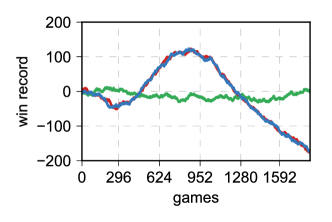
As an example of how the empirical series look like in Fig. 1 we have plotted win record series for SAC (Sacramento Kings). Additional curves in the figure show the examples of shuffled series. We will refer back to this figure when discussing shuffling algorithms in a more detail in the later sections of this paper.

Figure 1: (color online) Win record for SAC (red curve), single example of the fully shuffled win record for SAC (green curve) and single example of the in-season shuffled win record for SAC (blue curve).

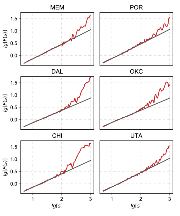
After running the original data through DFA, we have obtained results similar to those reported in [8]. We have found that $26$ of the $28$ teams exhibit persistent behavior as their $H>1/2$. Only DAL (Dallas Mavericks) and OKC (Oklahoma City Thunder/Seattle Supersonics) are within margin of error from $H=1/2$. For the detailed results see Table 1.

Table 1: Hurst exponents estimated for the win record time series of $28$ NBA teams in regular seasons 1995-2018

team	$H$	team	$H$	team	$H$
ATL	$0.5223\pm 0.0057$	IND	$0.528\pm 0.006$	PHI	$0.567\pm 0.005$
BKN	$0.5485\pm 0.0056$	LAC	$0.5455\pm 0.0057$	PHX	$0.5589\pm 0.0066$
BOS	$0.5311\pm 0.0067$	LAL	$0.5365\pm 0.0078$	POR	$0.5936\pm 0.0072$
CHI	$0.5456\pm 0.0077$	MEM	$0.5919\pm 0.0059$	SAC	$0.5242\pm 0.0073$
CLE	$0.561\pm 0.006$	MIA	$0.5771\pm 0.0083$	SAS	$0.5505\pm 0.0078$
DAL	$0.5016\pm 0.0051$	MIL	$0.5265\pm 0.0066$	TOR	$0.559\pm 0.005$
DEN	$0.5172\pm 0.006$	MIN	$0.5578\pm 0.0066$	UTA	$0.583\pm 0.007$
DET	$0.5186\pm 0.0073$	NYK	$0.5484\pm 0.0066$	WAS	$0.5354\pm 0.0065$
GSW	$0.5323\pm 0.0066$	OKC	$0.4960\pm 0.0051$
HOU	$0.5583\pm 0.0052$	ORL	$0.5687\pm 0.0068$

Note that for the most of the teams our $H$ estimates are smaller than those reported in [8]. This is because we have fitted $F\left(s\right)$ for $s\in\left[5,70\right]$, which is narrower interval than the one used in [8]. We prefer this narrower interval, because it is still comparatively broad (spans a bit over one order of magnitude) and the smallest $R^{2}$ over all teams in the data set is one of the largest obtained while considering other alternative intervals ($R^{2}=0.988$). $R^{2}$ reported in [8] is smaller which indicates that our fits are somewhat better. Also from a simple visual comparison it is pretty clear that the fits obtained in [8] are not very good (compare Fig. 2 in this paper and Fig. 1 in [8]). The slopes reported in [8] are somewhat larger than the ones reported by us, because their fitting interval is broader and includes $s>70$, while for the most of the teams $F\left(s\right)$ starts curve upwards for $s>70$, which inflates $H$ estimates. We believe that this curving upwards might indicate that there is another scaling regime, possibly related to the long-term decisions made on the season time scale ($82$ games). This curving upward might either be artifact observed due to the small sample size, or due to season-to-season persistence.

Figure 2: (color online) Quality of the fits, $F(s)\sim s^{H}$, provided by the reported Hurst exponents, Table 1, in the six selected cases: MEM and POR have the highest $H$ estimates, DAL and OKC have the lowest $H$ estimates, while CHI and UTA were used as examples in [8].

3 Checking the empirical results against random models

For small data sets, such as this one, estimation of the true underlying Hurst exponent using DFA (or other similar techniques) is not very reliable. E.g., in [21] MF-DFA, generalization of DFA, was used to estimate $H$ of synthetic series of various lengths, it was found that as small as $10^{4}$ points might be sufficient in some cases. [21] also lists numerous sophisticated bootstrap techniques, which preserve multifractal properties of the series. Yet our goals are simpler and for this paper it seems sufficient to use simple shuffling algorithms and also compare $H$ estimates against some simple random models. This section is dedicated to these tests. In all of the following tests our null hypothesis is that the data is neither persistent nor anti-persistent.

First of all let us shuffle all the games each team has played. This type of shuffling should remove persistence effects across all time scales. As can be seen in Fig. 1 the resulting shuffled win record series (green curve) is nothing alike the original series (red curve). We have shuffled team records $10^{4}$ times and have estimated $95\%$ confidence intervals (CIs) for what $H$ values could be reasonably expected to be obtained from a similar, yet non-persistent, series. If the estimated $H$ values are outside the obtained CIs, then for those cases we could reject the null hypothesis.

Table 2: Comparing $H$ estimates against CIs obtained from the fully shuffled data

Team	$H$	Shuffle CI	Reject the null?
ATL	$0.5223\pm 0.0057$	$[0.4667,0.5628]$	No
BKN	$0.5485\pm 0.0056$	$[0.4676,0.5640]$	No
BOS	$0.5311\pm 0.0067$	$[0.4675,0.5624]$	No
CHI	$0.5456\pm 0.0077$	$[0.4665,0.5639]$	No
CLE	$0.561\pm 0.006$	$[0.4657,0.5625]$	No
DAL	$0.5016\pm 0.0051$	$[0.4670,0.5630]$	No
DEN	$0.5172\pm 0.006$	$[0.4663,0.5637]$	No
DET	$0.5186\pm 0.0073$	$[0.4666,0.5637]$	No
GSW	$0.5323\pm 0.0066$	$[0.4673,0.5635]$	No
HOU	$0.5583\pm 0.0052$	$[0.4669,0.5626]$	No
IND	$0.528\pm 0.006$	$[0.4658,0.5640]$	No
LAC	$0.5455\pm 0.0057$	$[0.4661,0.5632]$	No
LAL	$0.5365\pm 0.0078$	$[0.4664,0.5640]$	No
MEM	$0.5919\pm 0.0059$	$[0.4675,0.5631]$	Yes
MIA	$0.5771\pm 0.0083$	$[0.4671,0.5631]$	Yes
MIL	$0.5265\pm 0.0066$	$[0.4660,0.5622]$	No
MIN	$0.5578\pm 0.0066$	$[0.4667,0.5633]$	No
NYK	$0.5484\pm 0.0066$	$[0.4672,0.5639]$	No
OKC	$0.4960\pm 0.0051$	$[0.4674,0.5630]$	No
ORL	$0.5687\pm 0.0068$	$[0.4674,0.5640]$	No
PHI	$0.567\pm 0.005$	$[0.4668,0.5635]$	No
PHX	$0.5589\pm 0.0066$	$[0.4658,0.5628]$	No
POR	$0.5936\pm 0.0072$	$[0.4674,0.5626]$	Yes
SAC	$0.5242\pm 0.0073$	$[0.4661,0.5639]$	No
SAS	$0.5505\pm 0.0078$	$[0.4684,0.5641]$	No
TOR	$0.559\pm 0.005$	$[0.4667,0.5627]$	No
UTA	$0.583\pm 0.007$	$[0.4676,0.5636]$	Yes
WAS	$0.5354\pm 0.0065$	$[0.4666,0.5631]$	No

As we can see in Table 2 we are able reject the null hypothesis in $4$ cases: for MEM (Vancouver/Memphis Grizzlies), MIA (Miami Heat), POR (Portland Trail Blazers) and UTA (Utah Jazz) the estimated $H$ is larger than would be expected if the series would be non-persistent. When analyzing $28$ cases under $5\%$ significance level we could reasonably expect to have $1$ or $2$ false rejections. Though these expectations do not account for the fact that the empirical series under consideration are not mutually independent, as a win for one team is a loss for another. In this context obtaining $4$ false rejections no longer seems unexpected. Thus we consider the obtained evidence questionable.

We can also check whether the streak lengths (first passage times) of the original and the shuffled series come from the different distributions. Note that for this test we use not the win record series (shown in Fig. 1), but the binary won-lost series. For the sake of consistency for this test we use only one shuffled time series per team. Here we use Kolmogorov-Smirnov test [22] with significance level $\alpha=0.05$. For the both winning and losing streaks we were able reject the null hypothesis (that the sets of streaks come from the same distribution) only for the winning streaks of MEM. As these results is within expected false rejection count, we consider the obtained evidence is negligible.

We can perform another test using the streak length distribution: whether the streak lengths from the original data are inconsistent with an independent randomness model. For this test we assume the following model: the team has probability $p_{w}$ to win each game independently of the other games and $p_{w}$ is estimated based on the overall win-loss record of the team. Once again here we have used only one randomly generated series. This time using Kolmogorov-Smirnov test ($\alpha=0.05$) we were able to reject the null hypothesis only for the winning streaks of LAL (Los Angeles Lakers). We consider this evidence to be negligible, as the rejection count is within the expected false rejection count.

This independent randomness model could be further simplified by ignoring the overall win-loss record (setting $p_{w}=0.5$ for all teams). But in this case the number of rejections is significantly higher: $4$ rejections for the winning streaks and $5$ rejections for the losing streaks. The increased rejection count is expected for the teams which won noticeably more or less than half of its games. What is striking is that the fully random model is consistent with records of the most teams, which could indicate that the technique is not sensitive enough to capture small differences in the probability to win a single game.

To further our discussion let us try a slightly different shuffling algorithm. This time let us shuffle the games inside the seasons, but preserve the ordering of the seasons. The in-season algorithm destroys the possible game-to-game persistence, but retains season-to-season persistence. An example of the series shuffled using this algorithm (blue curve) is shown in Fig. 1. As can be easily seen the blue curve repeats the general shape of the original (red) curve. Once again we have obtained $10^{4}$ shuffles and have estimated $95\%$ CIs for $H$ estimates. As we can see in Table 3 we are able to reject the null hypothesis in just two cases (POR and UTA). As these results is within expected false rejection count, we consider the obtained evidence is negligible.

Table 3: Comparing $H$ estimates against CIs obtained from the in-season shuffled data

team	$H$	In-season shuffle CI	Reject the null?
ATL	$0.5223\pm 0.0057$	$[0.4925,0.5825]$	No
BKN	$0.5485\pm 0.0056$	$[0.5067,0.5947]$	No
BOS	$0.5311\pm 0.0067$	$[0.5187,0.6043]$	No
CHI	$0.5456\pm 0.0077$	$[0.5284,0.6129]$	No
CLE	$0.561\pm 0.006$	$[0.5194,0.6056]$	No
DAL	$0.5016\pm 0.0051$	$[0.4773,0.5707]$	No
DEN	$0.5172\pm 0.006$	$[0.4916,0.5839]$	No
DET	$0.5186\pm 0.0073$	$[0.4834,0.5736]$	No
GSW	$0.5323\pm 0.0066$	$[0.4975,0.5859]$	No
HOU	$0.5583\pm 0.0052$	$[0.4968,0.5853]$	No
IND	$0.528\pm 0.006$	$[0.4853,0.5776]$	No
LAC	$0.5455\pm 0.0057$	$[0.4885,0.5835]$	No
LAL	$0.5365\pm 0.0078$	$[0.4910,0.5820]$	No
MEM	$0.5919\pm 0.0059$	$[0.4963,0.5867]$	No
MIA	$0.5771\pm 0.0083$	$[0.5125,0.5995]$	No
MIL	$0.5265\pm 0.0066$	$[0.4892,0.5793]$	No
MIN	$0.5578\pm 0.0066$	$[0.4881,0.5795]$	No
NYK	$0.5484\pm 0.0066$	$[0.4886,0.5800]$	No
OKC	$0.4960\pm 0.0051$	$[0.4917,0.5810]$	No
ORL	$0.5687\pm 0.0068$	$[0.4951,0.5858]$	No
PHI	$0.567\pm 0.005$	$[0.4995,0.5895]$	No
PHX	$0.5589\pm 0.0066$	$[0.5147,0.5994]$	No
POR	$0.5936\pm 0.0072$	$[0.4828,0.5768]$	Yes
SAC	$0.5242\pm 0.0073$	$[0.4752,0.5688]$	No
SAS	$0.5505\pm 0.0078$	$[0.5028,0.5899]$	No
TOR	$0.559\pm 0.005$	$[0.5000,0.5898]$	No
UTA	$0.583\pm 0.007$	$[0.4814,0.5744]$	Yes
WAS	$0.5354\pm 0.0065$	$[0.4893,0.5781]$	No

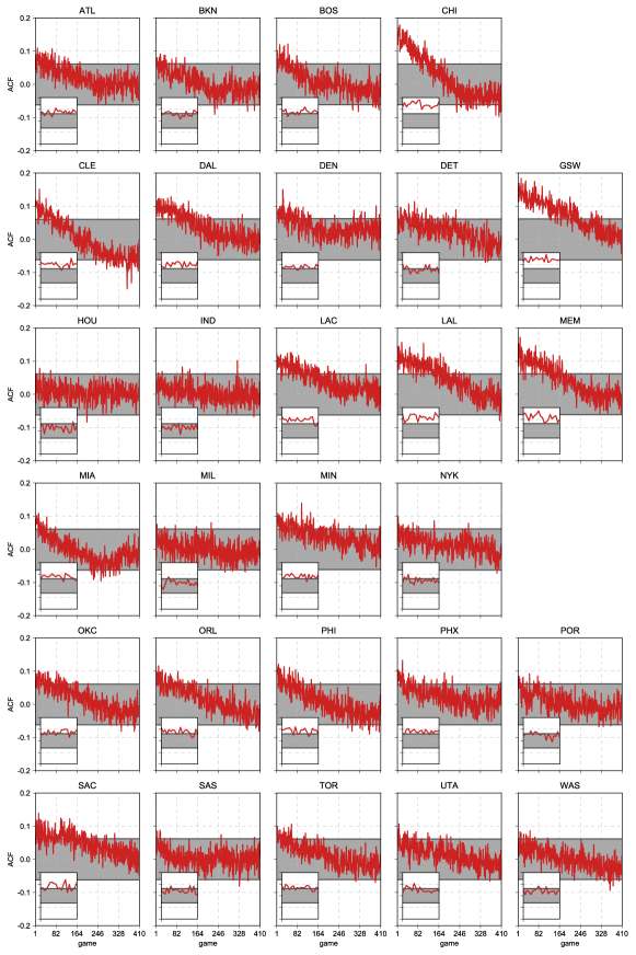
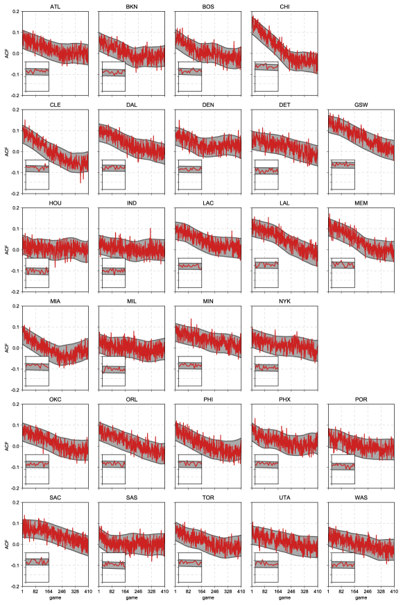
Another way to look at temporal persistence is to examine ACF of the series. In Fig. 3 we see that most of the teams have weakly positive ACFs for the lags up to $82$ games (one season). In quite a few cases, most notably CHI (Chicago Bulls) and GSW (Golden State Warrriors), the ACF is outside reasonably expected range (gray area) if the series would be random (comparison is made against the fully shuffled series). Yet the excess autocorrelation is well explained by taking season-to-season variations into account. In Fig. 4 the comparison is made against the in-season shuffled data and as one can see the empirical ACFs are now within the reasonably expected range (gray area).

Figure 3: (color online) Comparison between the autocorrelation functions of the empirical series (red curves) and the $95\%$ confidence intervals obtained by fully shuffling the respective empirical series (gray areas). Embedded subplots provide a zoom in on the x-axis (to $[1,20]$ games interval).

Figure 4: (color online) Comparison between the autocorrelation functions of the empirical series (red curves) and the $95\%$ confidence intervals obtained by shuffling the respective empirical series in-season (gray areas). Embedded subplots provide a zoom in on the x-axis (to $[1,20]$ games interval).

4 Conclusion

In our exploration of the NBA regular season data set from the period 1995-2018 we have not found enough evidence supporting the “winning streak” phenomenon. Although for the most of the teams we have obtained Hurst exponents larger than $0.5$ (these results are somewhat consistent with the ones reported in [8]), which would indicate the presence of persistence, these results are mostly consistent with the considered random models (full data shuffle, in-season data shuffle and independent randomness model) at significance level of $5\%$. It appears that the observed persistence is simply an illusion caused by the limited amount of data under consideration. Nevertheless DFA, as suggested by [8], seems to be an interesting tool to be applied to the sports time series and extensive application of it on a long time series could potentially provide arguments to the ongoing “hot hand” debate. Furthermore it seems that DFA could be also used to answer different question related to the different manegerial strategies teams use, e.g., in [19] it was examined whether religious practicies have impact on the baby birth times.

We have backed the results obtained using DFA technique by analyzing streak length distributions. Namely, using Kolmogorov-Smirnov test ($\alpha=0.05$), we were unable to find any evidence indicating that the empirical streak lengths would be inconsistent with the independent randomness model. These results also suggest that there is no evidence for the persistence in winning record, or the “winning streak”, phenomenon.

Analysis carried out using ACFs paints a more sophisticated picture. Empirical ACFs are not fully consistent with ACFs one would expect if there were no persistence. Yet these inconsistencies are well explained by retaining season-to-season variations. This would point to an obvious fact that long-term managerial decisions have an impact on team’s performance. While on the other hand short-term decisions and effects as “wining streaks” do not seem to have effects which would be inconsistent with random models.

Finally we would like to advise against gambling by relying on the persistence. Not only because we did not find sufficient evidence for the game-to-game persistence phenomenon in the NBA time series, but also because in the cases where persistence was detected (e.g., financial time series), there are still no reliable forecasting algorithms relying on the persistence alone. Gambling on the other hand could also influence the outcome of the games, but we would doubt if it had effect in as reputable league as NBA. It is likely that DFA or simple random models (similar to ones considered here) could be used to detect betting frauds in less reputable sports leagues.

We have made all of the scripts as well as the data, we have used in this analysis, freely available using GitHub [23].

References

- [1] T. Gilovich, “Judgmental biases in the world of sports.” in Cognitive sport psychology, W. F. Straub and J. M. Williams, Eds. Sport Science Associates, 1984.
- [2] T. Gilovich, R. Vallone, and A. Tversky, “The hot hand in basketball: On the misperception of random sequences,” Cognitive Psychology, vol. 17, pp. 295–314, 1985.
- [3] M. Bar-Eli, S. Avugos, and M. Raab, “Twenty years of hot hand research: Review and critique,” Psychology of Sport and Exercise, vol. 7, pp. 525–553, 2006.
- [4] P. Ayton and I. Fischer, “The hot hand fallacy and the gambler’s fallacy: Two faces of subjective randomness?” Memory & Cognition, vol. 32, no. 8, pp. 1369–1378, 2004.
- [5] D. L. Gilden and S. G. Wilson, “On the nature of streaks in signal detection,” Cognitive Psychology, vol. 28, pp. 17–64, 1995.
- [6] R. C. Vergin, “Winning streaks in sports and the mispeception of momentum,” Journal of Sport Behavior, vol. 23, no. 2, pp. 181–198, 2000.
- [7] B. Green and J. Zwiebel, “The hot-hand fallacy: Cognitve mistakes or equilibrium adjustments? Evidence from Major League Baseball,” in MIT Sloan Sports Analytics Conference 2016, 2016.
- [8] P. Ferreira, “What detrended fluctuation analysis can tell us about NBA,” Physica A, vol. 500, pp. 92–96, 2018. [Online]. Available: https://doi.org/10.1016/j.physa.2018.02.050
- [9] J. B. Miller and A. Sanjurjo, “Surprised by the gambler’s and hot hand fallacies? A truth in the law of small numbers,” IGIER Working Paper No. 552, 2016.
- [10] K. Ivanova and M. Ausloos, “Application of the detrended fluctuation analysis (DFA) method for describing cloud breaking,” Physica A, vol. 274, no. 1, pp. 349–354, 1999. [Online]. Available: http://www.sciencedirect.com/science/article/pii/S037843719900312X
- [11] J. W. Kantelhardt, E. Koscielny-Bunde, H. H. A. Rego, S. Havlin, and A. Bunde, “Detecting long-range correlations with detrended fluctuation analysis,” Physica A, vol. 295, no. 3, pp. 441–454, 2001. [Online]. Available: http://www.sciencedirect.com/science/article/pii/S0378437101001443
- [12] M. Ausloos and K. Ivanova, “Power-law correlations in the southern-oscillation-index fluctuations characterizing El Nino,” Physical Review E, vol. 63, p. 047201, 2001. [Online]. Available: https://link.aps.org/doi/10.1103/PhysRevE.63.047201
- [13] J. W. Kantelhardt, S. A. Zschiegner, E. Koscielny-Bunde, S. Havlin, A. Bunde, and H. E. Stanley, “Multifractal detrended fluctuation analysis of nonstationary time series,” Physica A, vol. 316, pp. 87–114, 2002.
- [14] M. Ausloos and K. Ivanova, “Multifractal nature of stock exchange prices,” Computer Physics Communications, vol. 147, pp. 582–585, 2002.
- [15] C. Peng, S. Buldyrev, S. Havlin, M. Simmons, H. E. Stanley, and A. Goldberger, “Mosaic organization of DNA nucleotides,” Physical Review E, vol. 49, pp. 1685–1689, 2004.
- [16] J. Kwapien, P. Oswiecimka, and S. Drozdz, “Components of multifractality in high-frequency stock returns,” Physica A, vol. 350, pp. 466–474, 2005.
- [17] G. Lim, S. Kim, H. Lee, K. Kim, and D.-I. Lee, “Multifractal detrended fluctuation analysis of derivative and spot markets,” Physica A, vol. 386, no. 1, pp. 259 – 266, 2007. [Online]. Available: http://www.sciencedirect.com/science/article/pii/S0378437107008138
- [18] Y.-H. Shao, G. F. Gu, Z.-Q. Jiang, W.-X. Zhou, and D. Sornette, “Comparing the performance of FA, DFA and DMA using different synthetic long-range correlated time series,” Scientific Reports, vol. 2, p. 835, 2012.
- [19] G. Rotundo, M. Ausloos, C. Herteliu, and B. Ileanu, “Hurst exponent of very long birth time series in XX century Romania. Social and religious aspects,” Physica A, vol. 429, pp. 109–117, 2015. [Online]. Available: http://www.sciencedirect.com/science/article/pii/S0378437115000989
- [20] J.-Y. Chiang, J.-W. Huang, L.-Y. Lin, C.-H. Chang, F.-Y. Chu, Y.-H. Lin, C.-K. Wu, J.-K. Lee, J.-J. Hwang, J.-L. Lin, and F.-T. Chiang, “Detrended Fluctuation Analysis of heart rate dynamics is an important prognostic factor in patients with end-stage renal disease receiving peritoneal dialysis,” PLOS ONE, vol. 11, no. 2, pp. 1–10, 02 2016.
- [21] S. Drozdz, J. Kwapien, P. Oswiecimka, and R. Rak, “Quantitative features of multifractal subtleties in time series,” European Physics Letters, vol. 88, p. 60003, 2009.
- [22] R. H. C. Lopes, Kolmogorov-Smirnov test. Springer, 2011, pp. 718–720. [Online]. Available: https://doi.org/10.1007/978-3-642-04898-2_326
- [23] A. Kononovicius, “Illusion of persistence in NBA 1995-2018 regular season data,” GitHub repository, 2018. [Online]. Available: https://github.com/akononovicius/