A New Look at T Tauri Star Forbidden Lines: MHD Driven Winds from the Inner Disk

Abstract

Magnetohydrodynamic (MHD) and photoevaporative winds are thought to play an important role in the evolution and dispersal of planet-forming disks. We report the first high-resolution ($\Delta v\sim$ 6  km s^-1) analysis of [S II] $\lambda$4068, [O I] $\lambda$5577, and [O I] $\lambda$6300 lines from a sample of 48 T Tauri stars. Following Simon et al. (2016), we decompose them into three kinematic components: a high-velocity component (HVC) associated with jets, and a low-velocity narrow (LVC-NC) and broad (LVC-BC) components. We confirm previous findings that many LVCs are blueshifted by more than 1.5  km s^-1  thus most likely trace a slow disk wind. We further show that the profiles of individual components are similar in the three lines. We find that most LVC-BC and NC line ratios are explained by thermally excited gas with temperatures between 5,000$-$10,000 K and electron densities $\sim 10^{7}-10^{8}$ cm^-3. The HVC ratios are better reproduced by shock models with a pre-shock H number density of $\sim 10^{6}-10^{7}$ cm^-3. Using these physical properties, we estimate $\dot{M}_{\rm wind}/\dot{M}_{\rm acc}$ for the LVC and $\dot{M}_{\rm jet}/\dot{M}_{\rm acc}$ for the HVC. In agreement with previous work, the mass carried out in jets is modest compared to the accretion rate. With the likely assumption that the NC wind height is larger than the BC, the LVC-BC $\dot{M}_{\rm wind}/\dot{M}_{\rm acc}$ is found to be higher than the LVC-NC. These results suggest that most of the mass loss occurs close to the central star, within a few au, through an MHD driven wind. Depending on the wind height, MHD winds might play a major role in the evolution of the disk mass.

1 Introduction

Circumstellar disks form as a result of angular momentum conservation during the protostellar core collapse (Shu, 1977) and play an important role both in star and planet formation. At early times, a significant fraction of the stellar mass is accreted through the disk and what is not accreted or dispersed via other mechanisms provide the raw material to build planets. As such it is important to understand how disks evolve and disperse.

In the current paradigm, there are three main stages of disk evolution and dispersal (e.g., Gorti et al. 2016, Ercolano & Pascucci 2017 for recent reviews). For most of the disk lifetime (Stage 1), evolution is primarily set by accretion. Beyond a fraction of the radius where the sound speed equals the local Keplerian orbital speed ($\sim 2$ au for $10^{4}$ K gas, and $\gtrsim 10-100$ au for $100-1,000$ K gas for a sun-like star) gas becomes unbound and a photoevaporative thermal wind can be established. When the disk accretion rate through this radius drops below the wind mass loss rate, photoevaporation limits the supply of gas to the inner disk, a gap is formed (Stage 2), and the inner disk drains onto the star on the local viscous timescale - of order 100,000 years. In the last stage (Stage 3), there is no accretion onto the star and the disk is rapidly cleared from inside-out by stellar high-energy photons directly irradiating the outer disk.

Although photoevaporative winds are believed to play an important role in disk dispersal, large scale jets/outflows, which contribute to significant mass loss at the earliest stages, are usually attributed to an origin in an MHD wind (e.g., Frank et al. 2014 for a recent review). Such winds can be effective in removing disk angular momentum and in facilitating accretion of disk gas onto the star (e.g., Pudritz et al. 2007; Shang et al. 2007).

Recently, significant theoretical effort has been devoted to understanding MHD disk winds and their relation to accretion and disk dispersal. It has long been realized that the inclusion of non-ideal MHD effects suppresses magnetorotational instability (MRI) turbulence (e.g., Gammie 1996) and recent numerical simulations show that even a weak net vertical magnetic field, which could be for example leftover from the earlier stage of cloud collapse, can drive MHD winds (e.g., Suzuki & Inutsuka 2009, Fromang et al. 2013). Local box simulations (e.g., Bai & Stone 2013) and radially global, but vertically restricted, simulations (Gressel et al., 2015; Béthune et al., 2017) show that the launch of MHD winds is robust, can occur over the planet-forming region ($\sim$ 1–30 au), and can drive accretion at the observed levels. However, the predicted wind mass loss rate, hence the accretion rate, strongly depends on the magnetic field strength and how it evolves (e.g., Armitage et al. 2013, Bai & Stone 2017), both of which are poorly constrained. Therefore, identifying diagnostics that trace disk winds and deriving wind mass loss rates is important not only to understand how disks disperse but also how they evolve.

Low-excitation optical forbidden lines, especially from the [O I] $\lambda$6300 transition, have long been used to study jets/outflows from T Tauri stars (e.g., Edwards et al. 1987; Hartigan et al. 1995). Their line profiles typically present two distinct components: a high-velocity component (HVC), blueshifted by 30–200  km s^-1 from the stellar velocity, and a low-velocity component (LVC), typically blueshifted by $\sim$5  km s^-1. Spatially resolved observations have demonstrated that HVCs are formed in extended collimated jets (e.g., Lavalley-Fouquet et al. 2000; Bacciotti et al. 2000; Woitas et al. 2002), most likely linked to MHD winds (e.g., Ferreira et al. 2006).

Employing much higher spectral resolution than in previous studies ($\Delta v\sim$ 4  km s^-1), Rigliaco et al. (2013) found that the [O I] LVC itself can be described by the combination of a narrow component (NC) and a broad component (BC). More recently, Simon et al. (2016) confirmed this finding on a much larger sample of 33 T Tauri stars observed with Keck/HIRES ($\Delta v\sim$ 7  km s^-1). Using the line profiles and inclinations from resolved disk images, they inferred that most of the LVC-BC arises within $\sim 0.5$ au while most of the LVC-NC arises outside this radius. By combining measured velocities with line widths and disk inclinations, they also found that the LVC-BC tend to be narrower and more blueshifted for closer to face-on disks, as shown in some disk wind models (e.g., Alexander 2008). Finally, since the emitting region is within the photoevaporating radius even for 10,000 K gas, they could conclude that the LVC-BC traces an MHD disk wind. The origin of the LVC-NC remains unclear as the inferred radial extent is consistent with a thermally driven photoevaporative wind but no trend between blueshifts and disk inclinations was seen (Simon et al., 2016).

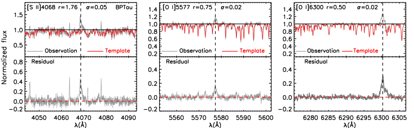
Figure 1: Top: Example of the removal of telluric (only for [O I] $\lambda$6300) and photospheric absorption features near [S II] $\lambda$4068, [O I] $\lambda$5577, and [O I] $\lambda$6300 lines for BP Tau. In each panel, the normalized target spectrum is shown in gray. The telluric and photospheric absorption features have not been removed from the spectrum. The best-fit photospheric template is shown in red, and used to subtract the photospheric absorption features (including the telluric absorption features for [O I] $\lambda$6300) from the target spectrum. Bottom: the final corrected line profiles of [S II] $\lambda$4068, [O I] $\lambda$5577, and [O I] $\lambda$6300 of BP Tau.

An important step in computing wind mass loss rates is to constrain the properties of the emitting gas associated with the wind. Ratios of lines tracing the same kinematic component can be employed for this task (e.g., Dougados et al. 2010). However, so far the only lines analyzed at similarly high spectral resolution to distinguish BC and NC are the [O I] $\lambda$6300 and [O I] $\lambda$5577. Assuming that the lines are thermally excited their ratios constrain the range of temperature-electron densities for the emitting gas and imply higher electron density in the region traced by the LVC-BC for gas at similar temperatures (Simon et al., 2016). However, FUV photodissociation of OH molecules can produce a similar range of [O I] ratios in much cooler ($\sim$1,000 K) gas (e.g., Harich et al. 2000 and Gorti et al. 2011 for an application to disks). In this scenario of non-thermal emission, line ratios do not constrain the temperature and density of the gas. In order to estimate wind mass loss rates, it is therefore necessary to first establish that the [O I] $\lambda$6300 and [O I] $\lambda$5577 emission is thermal. As first pointed out in Natta et al. (2014), the [S II] $\lambda$4068 has a critical density very similar to the [O I] $\lambda$6300 line and is likely to be thermally excited, hence the [S II] and [O I] line profiles, as well as their line ratio, can be used to distinguish between thermal vs non-thermal excitation.

In this work, we expand upon previous high-resolution studies by analyzing the [S II] $\lambda$4068, [O I] $\lambda$5577, and [O I] $\lambda$6300  from a sample of 48 T Tauri stars with the main goal of determining whether the [O I] emission is thermal or non-thermal. In a parallel work, we focus on the kinematic behavior of individual [O I] components to clarify the link between jets and winds (Banzatti et al. 2018). First, we describe our sample, observations, and data reduction ($\S$2). Then, we present our analysis ($\S$3), which includes line decomposition in HVC LVC-BC, and LVC-NC following Simon et al. (2016). In $\S$4 we show that the [S II] $\lambda$4068, [O I] $\lambda$5577, and [O I] $\lambda$6300 line profiles are very similar within each kinematic component strongly suggesting that the [O I] emission is thermally produced, and not the result of photodisocciation of OH in a cool gas. We use line ratios to constrain the properties of the emitting gas and compute wind mass loss rates in $\S$5. We also calculate mass accretion rates from several permitted lines and compare accretion vs mass loss rates ($\S$5). We discuss the implications of our results in $\S$6 and summarize our findings in $\S$7.

2 Sample and Data Reduction

Table 1: A list of the sources in this work, as well as their stellar and disk properties and the used photspheric templates

ID	Name	Region	Dist	Spt	Log $L_{\star}$	$A_{\rm V}$	$R_{\star}$	$M_{\star}$	Disk	$i$	Ref	RV(Helio)	Correction	Photospheric template
			(pc)	Type	($L_{\odot}$)	(mag)	($R_{\odot}$)	($M_{\odot}$)		(deg)		( km s-1)	( km s-1)	[S II] $\lambda$4068	[O I] $\lambda$5577, [O I] $\lambda$6300
1	DP Tau	Taurus	130	M0.8	$-1.24$	0.80	0.56	0.55	Full		1	16.55$\pm$0.89	$-0.64$	no correction	TWA 13
2	CX Tau	Taurus	126.8	M2.5	$-0.61$	0.25	1.36	0.35	TD	61	1, 9	19.15$\pm$1.31	$-0.40$	$\cdots$	TWA 8A
3	FP Tau	Taurus	127.2	M2.6	$-0.81$	0.60	1.10	0.35	TD	66	1, 9	16.90$\pm$2.11	$-0.75$	TWA 8A	TWA 8A
4	FN Tau	Taurus	129.7	M3.5	$-0.29$	1.15	2.22	0.24	Full		1	16.29$\pm$1.23	$-0.09$	TWA 8A	TWA 8A
5	V409 Tau	Taurus	130.2	M0.6	$-0.19$	1.00	1.87	0.47	Full		1	17.78$\pm$0.73	$-0.49$	TWA 13	TWA 13
6	BP Tau	Taurus	127.7	M0.5	$-0.40$	0.45	1.45	0.54	Full	39	1, 10	16.76$\pm$0.54	$-0.43$	TWA 13	V819 Tau
7	DK Tau A	Taurus	127.1	K8.5	$-0.35$	0.70	1.41	0.66	Full	26	1, 11	16.60$\pm$0.42	$-0.71$	TWA 13	V819 Tau
8	HN Tau A	Taurus	133.3	K3	$-0.81$	1.15	0.63	0.69	Full	75	1, 9	18.91$\pm$1.96	$-0.46$	no correction	2MASS J15584772-1757595
9	UX TauA	Taurus	137.5	K0	$0.18$	0.65	1.74	1.40	TDa	39	1, 11	18.80$\pm$0.64	$-0.44$	EPIC 212021375b	EPIC 203476597
10	GK TauA	Taurus	128.1	K6.5	$-0.11$	1.50	1.78	0.67	Full	71	1, 9	18.52$\pm$0.64	$-0.49$	HD 201092b	V819 Tau
11	GI Tau	Taurus	129.2	M0.4	$-0.32$	2.05	1.58	0.53	Full		1	19.02$\pm$0.55	$-0.40$	TWA 13	V819 Tau
12	DM Tau	Taurus	143.5	M3.0	$-0.87$	0.10	1.05	0.31	TDa	34	1, 11	19.64$\pm$1.50	$-1.36$	TWA 8A	TWA 8A
13	LKCa 15	Taurus	156.9	K5.5	$-0.11$	0.30	1.69	0.76	TDa	51	1, 11	18.71$\pm$0.46	$-0.55$	HD36003b	V819 Tau
14	DS Tau	Taurus	157.2	M0.4	$-0.62$	0.25	1.12	0.62	Full	71	1, 9	16.51$\pm$0.97	$-0.28$	TWA 13	TWA 13
15	SZ 65	Lupus	153.4	K6	$-0.03$	0.80	1.90	0.68	TD	61	1, 19	$-$2.85$\pm$0.90	$-0.60$	HD 36003b	V819 Tau
16	SZ 68A	Lupus	152.1	K2	$0.75$	1.00	3.57	1.27	Full	33	1, 19	$-$1.41$\pm$1.28	$-0.74$	EPIC 212021375b	2MASS J15584772-1757595
17	SZ 73	Lupus	154.8	K8.5	$-0.74$	2.75	0.90	0.75	Full	50	1, 12	$-$3.56$\pm$1.59	$-1.10$	HD 201092b	V819 Tau
18	HM Lup	Lupus	154.1	M2.9	$-0.78$	0.60	1.16	0.32	Full	53	1, 12	$-$1.62$\pm$1.82	$-0.90$	TWA 8A	TWA 8A
19	GW Lup	Lupus	153.9	M2.3	$-0.61$	0.55	1.34	0.37	Full	40	1, 12	$-$1.17$\pm$1.12	$-0.77$	TWA 8A	TWA 8A
20	GQ Lup	Lupus	150.1	K5.0	$-0.04$	1.60	1.80	0.78	Full	60	1, 13	$-$2.13$\pm$0.29	$-1.00$	HD 36003b	V819 Tau
21	SZ 76	Lupus	157.5	M3.2	$-0.69$	0.90	1.33	0.28	TDa		1	$-$1.14$\pm$2.16	$-1.01$	TWA 8A	TWA 8A
22	RU Lup	Lupus	157.2	K7.0	$0.16$	0.00	2.48	0.55	Full	3	2, 19	$-$0.8$\pm$2	$-0.98$	no correction	V819 Tau
23	IM Lup	Lupus	156.4	K6.0	$0.01$	0.40	1.98	0.67	TD	48	1, 19	$-$0.64$\pm$0.58	$-1.18$	HD 36003b	V819 Tau
24	RY Lup	Lupus	156.6	K2	$0.26$	0.40	2.02	1.27	Full	68	3, 22	$-$0.43$\pm$1.09	$-0.90$	EPIC 212021375b	EPIC 203476597
25	Sz 102	Lupus	160	K2	$-2.02$	0.70	0.15	$\cdots$	Full	73	3, 20	12$\pm$2	$-1.82$	no correction	no correction
26	Sz 111	Lupus	156.9	M1.2	$-0.69$	0.85	1.11	0.50	TDa	53	1, 22	$-$0.16$\pm$0.74	$-1.32$	HD 209290b	V819 Tau
27	Sz 98	Lupus	154.3	M0.4	$-0.49$	1.25	1.30	0.58	Full	47	1, 19	$-$0.32$\pm$0.70	$-0.86$	TWA 13	TWA 13
28	EX Lup	Lupus	157.0	M0	$-0.12$	1.1	2.04	0.44	Full	38	3, 28	2$\pm$1	$-0.88$	no correction	V819 Tau
29	AS 205A	$\rho$ Oph	125.9	K5	$0.89$	1.75	5.26	0.68	Full	25	1, 4, 14	$-$5.31$\pm$0.55	$-1.78$	HD 36003b	V819 Tau
30	DoAr 21	$\rho$ Oph	132.6	G1	$1.32$	7.10	4.50	2.79	TDa		1	$-$1.63$\pm$2.44	$-1.46$	$\cdots$	EPIC 203476597
31	DoAr 24E	$\rho$ Oph	135.7	K0	$0.20$	4.32	1.76	1.41	Full	20	5, 30	$-$5.77$\pm$0.60	$-1.66$	$\cdots$	EPIC 203476597
32	DoAr 44	$\rho$ Oph	144.3	K2	$-0.03$	1.7	1.45	1.22	TDa	16	6, 11	$-$4.50$\pm$0.53	$-1.50$	EPIC 212021375b	2MASS J15584772-1757595
33	EM* SR 21A	$\rho$ Oph	136.8	F7	$0.98$	6.2	2.62	1.79	TDa	18	1, 11, 15, 16	$-$5.66$\pm$3.65	$-1.41$	HIP 42106b	HIP 42106b
34	V853 Oph	$\rho$ Oph	138	M2.5	$-0.30$	0.14	1.95	0.32	Full	54	5, 11	$-$5.8$\pm$1.10	$-1.96$	TWA 8A	TWA 8A
35	RNO 90	$\rho$ Oph	115.7	G8	$0.42$	4.3	2.01	1.68	Full	37	17, 30	$-$9.11$\pm$1.09	$-1.70$	KW27b	EPIC 203476597
36	V2508 Oph	$\rho$ Oph	122.7	K7	$-0.13$	1.7	1.78	0.63	Full	41	17, 11	$-$7.62$\pm$0.79	$-1.94$	HD 201092b	V819 Tau
37	V1121 Oph	$\rho$ Oph	119.7	K4	$-0.06$	1.08	1.62	0.96	Full	31	5, 11	$-$6.27$\pm$0.32	$-1.78$	HD 36003b	TWA 9A
38	RX J1842.9$-$3532	Corona Australis	152.2	K3	$-0.23$	0.6	1.24	1.07	TDa	54	1, 18	$-$0.92$\pm$0.53	$-1.31$	HD 36003b	2MASS J15584772-1757595
39	RX J1852.3$-$3700	Corona Australis	144.1	K4	$-0.40$	0.25	1.10	0.96	TDa	16	1, 18	0.64$\pm$0.53	$-1.16$	HD 36003b	2MASS J15584772-1757595
40	VV CrA	Corona Australis	146.6	K7	$0.32$	3.95	2.99	0.53	Full	49	1, 21	$-$1.0$\pm$1	$-1.39$	no correction	V819 Tau
41	SCrA A+B	Corona Australis	150.3	K6	$0.24$	0.5	2.58	0.61	Full	10	8, 30	1.41$\pm$2.42	$-1.00$	no correction	2MASS J15584772-1757595
42	TW Hya	TWA	59.8	M0.5	$-0.63$	0.00	1.11	0.61	TDa	7	1, 11	13.55$\pm$0.34	$-1.24$	TWA 13	V819 Tau
43	TWA 3A	TWA	36.4	M4.1	$-1.19$	0.05	0.85	0.16	TD		1	11.84$\pm$2.52	$-0.83$	TWA 7	TWA 7
44	V1057 Cygc	Cygnus	897.7	$\sim$G0$?$	2.47	4.63			Full		23, 17	$-14.3\pm 1$	$-1.17$	no correction	EPIC 203476597
45	V1515 Cygc	Cygnus	980.8	$\sim$G3$?$	2.01	2.93			Full		24, 25, 17	$-11.13\pm 0.53$	$-1.40$	no correction	2MASS J15584772-1757595
46	HD 143006a	Upper Sco	165.5	G3	0.50	0.45	1.81	1.52	TDa	$\sim$28	1, 17, 29	$-0.19\pm 0.21$	$-1.30$	KW27b	KW541b
47	DI Cep	Cepheus	430.0	G8	0.85	0.25	3.27	2.28	Full		26, 17	$-7.00\pm 0.56$	$-2.36$	KW27b	EPIC 203476597
48	As 353A	LDN 673	404.0	K5	0.51	0.00	3.50	0.60	Full		27, 17	$-7.87\pm 0.60$	$-1.10$	no correction	HBC 427

Note: ^a listed as the TDs in van der Marel et al. (2016); ^b main sequence templates; ^c The stellar masses and radii for the two FU Ori are unknown since their spectral types are very uncertain. References: 1. Herczeg & Hillenbrand (2014), 2. Alcalá et al. (2014), 3. Alcalá et al. (2017), 4. Luhman & Mamajek (2012), 5. Sartori et al. (2003), 6. Manara et al. (2014), 7. Wahhaj et al. (2010), 8. Johns-Krull et al. (2000), 9 Simon et al. (2017), 10. Guilloteau et al. (2011), 11. Tripathi et al. (2017), 12. Ansdell et al. (2016), 13. MacGregor et al. (2017), 14. Andrews et al. (2010), 15. Najita et al. (2015), 16. van der Marel et al. (2016), 17. This work, 18. Hughes et al. (2010), 19. Tazzari et al. (2017), 20. Louvet et al. (2016), 21. Scicluna et al. (2016), 22. van der Marel et al. (2018), 23. Herbig et al. (2003), 24. Herbig (1977), 25. Herbig & Bell (1988), 26. Cohen & Kuhi (1979), 27. Rice et al. (2006), 28. Hales et al. (2018), 29. Lazareff et al. (2017), 30. Pontoppidan et al. (2011)

2.1 Sample

Our sample comprises 48 young stars with disks, see Table 1. Most of them belong to the following five star-forming regions and associations: Taurus, Lupus I, Lupus III, $\rho$ Oph, and Corona Australis. The TW Hya and Upper Sco associations have an average age of 5–10 Myr (Fang et al., 2013b; Donaldson et al., 2016; Fang et al., 2017) while all other regions are younger, with ages 1–3 Myr (Luhman et al., 2009; Frasca et al., 2017; Luhman & Rieke, 1999; Sicilia-Aguilar et al., 2011). We retrieve Gaia Data Release 2 parallactic distances for 47 of them from the geometric-distance table provided by Bailer-Jones et al. (2018). No parallax is reported for DP Tau, hence we adopt the median distance of nearby Taurus members which is $\sim$130 pc. With these new distances, Sz 102 is two times farther away than other Lupus members while V853 Oph is $\sim$50 pc closer than the $\rho$ Oph star-forming region. However, we note that both sources have high Astrometric Excess Noise in Gaia DR2 (2.881 and 5.944 for Sz 102 and V853 Oph, respectively), indicating that their astrometric solution is unreliable (Lindegren et al., 2018). Therefore, for these two sources we take the mean distance to Lupus III and $\rho$ Oph. Using stellar members collected by Alcalá et al. (2017) for Lupus and Manara et al. (2015) for $\rho$ Oph, we find 160 pc for Sz 102 and 138 pc for V853 Oph.

In addition to source distance and association, Table 1 also lists stellar spectral type, visual extinction ($A_{\rm V}$), luminosity, radius and mass ($L_{\star}$, $R_{\star}$, $M_{\star}$), disk type and inclination ($i$), and corresponding references. Note that stellar luminosities from the literature have been scaled to the new distances in our table. Stellar radii are calculated from the Stefan-Boltzman equation where the effective temperature is derived from the source spectral type according to the spectral type-effective temperature relation in Herczeg & Hillenbrand (2014). Stellar masses are calculated from the luminosity and effective temperature using the non-magnetic pre-main sequence evolutionary tracks of Feiden (2016). Our sample covers a large range in spectral type (F7 to M4), hence in stellar mass, from $\sim$2.8 to $\sim$0.2 $M_{\odot}$. Note that the two sources in Cygnus (V1057 Cyg and V1515 Cyg) are well known FU Ori objects, young stars showing strong episodic accretion bursts (e.g., Audard et al. 2014).

On the disk type, we distinguish "Full disks" from "Transitional disks" (TDs). TDs are known to have reduced near- and mid-infrared excess emission with respect to the median of T Tauri stars pointing to a dust depleted inner region (e.g., Espaillat et al., 2014). Hence, we classify our sources by comparing the source spectral energy distribution (SED) to the median SEDs of CTTs of similar spectral type, see Appendix A for details. With our approach we identify 28 full disks and 15 TDs. The 5 disks we could not classify are around G and F stars. As these stars are rare and their disks disperse faster (e.g., Kennedy & Kenyon, 2009), we simply lack a median SED for this spectral type range. For SR 21A and HD 143006 we adopt the literature classification of TDs (Najita et al., 2015; van der Marel et al., 2016). As there is no hint of reduced infrared emission in the SED of the other three G-type stars (V1057 Cyg, V1515 Cyg, and DI Cep) we classify their disks as full. Recently, van der Marel et al. (2016) used color criteria and SED modeling to identify a large sample of TD candidates in nearby star-forming regions. Of the 14 sources in common 13 are classified in the same way. Only FN Tau is classified as full disk here but listed as TD in van der Marel et al. (2016). Note, however, that van der Marel et al. (2016) estimate an uncertainty on the cavity size that is as large as the cavity itself, hence FN Tau might actually have a full disk as we adopt here.

2.2 Observations and data reduction

Our targets were observed during two nights, January 23 and May 23 2008, through the program C199Hb (PI: Greg J. Herczeg). The Keck/HIRES spectrograph (Vogt et al., 1994) was used with the C1 decker and a 0$\farcs$861$\times$7^′′ slit resulting in a nominal resolution of 48,000. The sources were observed with the kv380 filter, wavelength coverage 3900–8500 Å, during the night of January 23 and with the wg335 filter, wavelength coverage 3480–6310 Å, during the night of May 23. In addition to the science targets, three telluric standards at least were observed each night. These standards are used to correct for telluric features (Sect.  3.1) near the [O I] $\lambda$6300  line as well as for flux calibration (Appendix B).

The raw data were reduced using the Mauna Kea Echelle Extraction (MAKEE) pipeline written by Tom Barlow. MAKEE is designed to run non-interactively using a set of default parameters, and carry out bias-subtraction, flat-fielding, and spectral extraction, including sky subtraction, and wavelength calibration with ThAr calibration lamps. The wavelength calibration is performed in air by setting the keyword "novac" in the pipeline inputs. Heliocentric correction is also applied to the extracted spectra.

2.3 Stellar Radial velocity

The stellar radial velocity (RV) is derived by cross-correlating each star optical spectrum with the synthetic spectrum of a star that has the same effective temperature. The grid of model spectra is from Husser et al. (2013) for a solar abundance and surface gravity log $g$=4.0. The model spectrum is first degraded to match the spectral resolution of HIRES, rotationally broadened to match the source photospheric features, and ’veiled’ by adding a constant flux value to account for the fact that photospheric lines from T Tauri stars are less deep than those of main-sequence stars of the same spectral type. The cross-correlation is carried out separately for each echelle order that does not have strong emission lines or is highly veiled. Hence, the total number of available orders varies from source to source but it is at least 5, except for RU Lup, EX Lup, and V1057 Cyg. For RU Lup, we only detect photospheric features near the [O I] $\lambda$6300 line and use them to estimate the stellar radial velocity. For EX Lup, we detect photospheric features within 5733–5745 Å and 5936–5948 Å and the cross-correlation is performed within these wavelength ranges. The stellar radial velocity of V1057 Cyg is obtained by cross-correlating the observed spectrum with the model spectrum within 5556–5580 Å and 5645–5673 Å. Table 1 provides the stellar RV and associated uncertainty computed as the mean and standard deviation of the RVs obtained from individual orders.

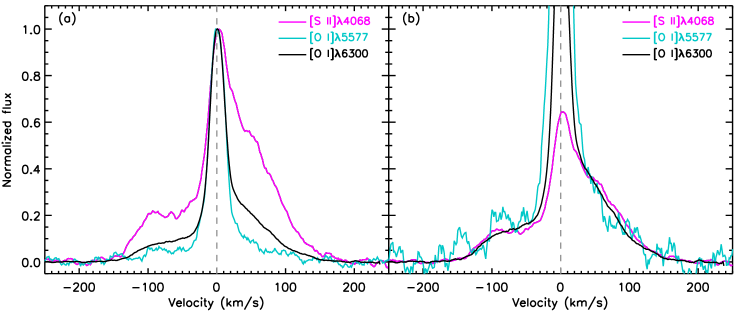
Figure 2: Comparison of [S II] $\lambda$4068 (magenta), [O I] $\lambda$5577 (cyan), and [O I] $\lambda$6300 (black) line profiles for DP Tau. The line profiles are scaled to show the similar velocity structure in the narrow core and broad wings among all three lines.

Sz 102 and VV CrA have highly veiled spectra with strong emission lines, hence no HIRES order can be used to derive their RVs. For these two sources, we download archival ESO Phase 3 X-Shooter spectra, which are wavelength and flux calibrated and have a resolution of $\sim$17,400 between 5,500–10,000Å. For VV CrA, we derive its RV by fitting its Li I $\lambda$6708 absorption line with a Gaussian function as in Pascucci et al. (2015). For Sz 102, we cannot clearly identify the Li I $\lambda$6708 absorption line, hence we derive its RV by cross-correlating the observed spectrum with the model spectrum within 7485–7530Å, 8020–8112Å, and 8762–8845Å where we can identify photospheric absorption lines. The RVs of these two sources are also listed in Table 1.

Note that synthetic spectra are only used for the computation of stellar RVs. As discussed in the next section, photospheric subtraction is carried out mostly with the observed spectra of weak-line T Tauri stars (WTTS). We do not have WTTS templates for 18 sources in the [S II] $\lambda$4068 setting and for one source, SR 21A (F7), around the [O I] $\lambda$6300 and the [O I] $\lambda$5577 settings, hence we used the main sequence (MS) templates in these instances, see Table 1.

Arc calibration frames for the absolute wavelength solution were taken only at the beginning of each night. Therefore, systematic shifts on the wavelength solution are possible when moving the telescope. We assess these possible shifts by cross-correlating the telluric lines with the model atmospheric transmission curve for the Keck Observatory which is calculated with TAPAS (a web-based service of atmospheric transmission computation for astronomy, see Bertaux et al. 2014). We find that the wavelength calibration tends to be redshift by $\sim$0.5–2  km s^-1. In Table 1, we list the RV correction for each source. Except for Sz 102 and VV CrA, whose RVs are estimated from X-Shooter spectra, the RVs of all other sources need to be corrected by adding the values in the "Correction" column to their RVs. However, the corrections only affect the heliocentric radial velocity derived from the HIRES spectra. They do not change the relative shifts between the stellar photospheric absorption features and the forbidden lines, which are the focus of this paper. We list these corrections in case one wants to compare the RVs calculated here with those obtained via other methods.

3 Line Profiles and Classification

3.1 Corrected line profiles and detection rates

To produce corrected line profiles, we first remove any telluric absorption and then subtract the photospheric features near the lines. Telluric removal is only necessary for the [O I] $\lambda$6300 line and is achieved with the procedure summarized in the HIRES Data Reduction manual and using the telluric standards acquired in the two nights.

After telluric removal, we subtract the stellar photosphere following Hartigan et al. (1989). In short, we select a photospheric standard with a spectral type similar to the target. We then broaden (through the rotation velocity $Vsini$), veil (parameter $r_{\lambda}$), and shift in velocity its spectrum to best match the target’s photospheric lines. Veiling is defined as the ratio of the excess ($F_{\rm excess}$) to the photospheric flux ($F_{\rm phot}$): $r_{\lambda}=F_{\rm excess}/F_{\rm phot}$ and it is used to mimic the filling in of the photospheric lines due to the excess emission from the accretion shocks. The best-fit photospheric spectrum is the one that minimizes the $\chi^{2}$, defined as $\chi^{2}=\sum(F_{\rm target}-F_{\rm Standard})^{2}$. Corrected line profiles are produced by subtracting the best-fit photospheric spectra from the target spectra. We do not apply any photospheric subtraction on extremely veiled spectra that have no photosheric features, e.g. several of the spectra in the [S II] $\lambda$4068 setting. Figure 1 shows an example of the technique described here, including telluric removal near the [O I] $\lambda$6300 Å line (rightmost panel). Table 1 lists the photospheric standards used for individual lines.

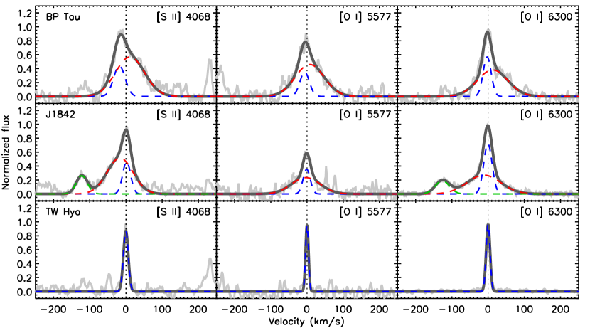
Figure 3: Examples of [S II] $\lambda$4068 , [O I] $\lambda$6300 , and [O I] $\lambda$5577 line profile fits. A green dashed line is used for the HVC, a red dashed line for the LVC-BC, while a blue dashed line for the LVC-NC. The dark solid line is the sum of the individual components. Line profile fits for all sources are shown in Fig. 20.

Overall, we detect the [O I] $\lambda$6300, the [O I] $\lambda$5577, and the [S II] $\lambda$4068  lines from 45, 26, and 22 sources, respectively. Hence, the detection rate is 92%, 54%, and 49% in these lines. A total of 18 sources have detections in all three lines.

3.2 Line decomposition

As recently shown in Simon et al. (2016), oxygen forbidden lines can be well reproduced by the superimposition of a few Gaussian profiles, presumably tracing different kinematic components. Figure 2 compares the [S II] $\lambda$4068, [O I] $\lambda$5577, and [O I] $\lambda$6300 emission lines from DP Tau, one of the sources with the highest S/N spectra. Note how a narrow component centered at the stellar velocity is present in all lines (panel a). Broader higher velocity emission is also apparent in the three tracers (Panel b).

Motivated by the similarity of the profiles in the high S/N spectrum of DP Tau and following Simon et al. (2016), we use a combination of Gaussians to decompose the [S II] $\lambda$4068, [O I] $\lambda$5577, and [O I] $\lambda$6300  lines. To find the minimum number of Gaussians that describes the observed profile, we use an iterative approach based on the IDL procedure mpfitfun. We start by fitting each profile with one Gaussian and compute the residual spectrum by subtracting the best fit from the original profile. If the root mean square (rms) of the residual is higher than that of the original spectrum next to the line of interest (by more than $\sim$2$\sigma$), we add another Gaussian and re-fit the original profile simultaneously with two Gaussians. We re-compute the residual spectrum and add an extra Gaussian until the rms of the residual is within 2$\sigma$ of the rms of the original spectrum.

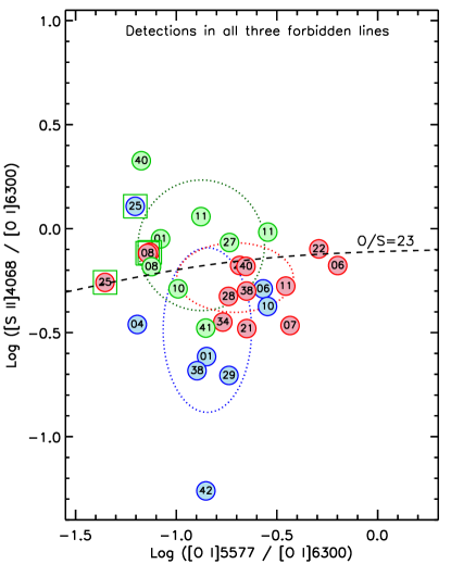
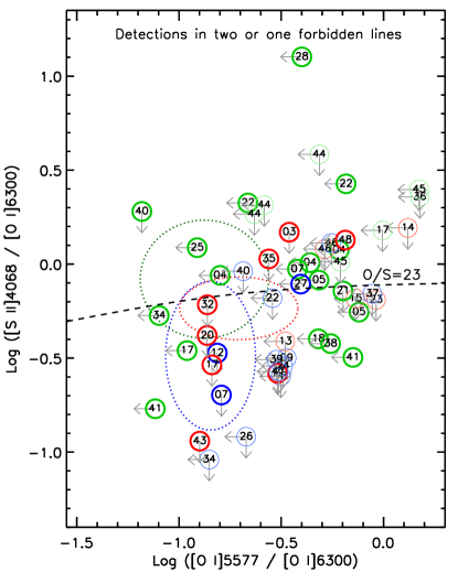
Figure 4: Line ratios with colors following the preliminary classification: green for HVC, red for LVC-BC, and blue for LVC-NC. The number inside the circle gives the source ID as listed in Table 1. Left panel: only sources that are detected in all three forbidden lines. Dotted-line ellipses encircle the mean $\pm$ standard deviation of the HVCs (green), LVC-BCs (red), and LVC-NCs (blue) from the preliminary classification. Green squares mark those LVC-BCs that are re-classified as HVCs. Right panel: like the left panel but for sources that are detected in two forbidden lines (thick-line circles) and only in the [O I] $\lambda$6300 line (thin-line circles). In both panels the black dashed line shows predicted ratios for 10⁴ K gas, assuming an Oxygen to Sulfur abundance ratio of 23, where collisions with electrons (densities $10^{5.8-8.5}$ cm^-3) excite the upper levels of the transitions, see Sect.  4.2.1 for more details.

Table 2 lists the parameters resulting from the decomposition of each individual line while Figure 3 shows examples of the best fit Gaussian profiles for three sources. All other fits are shown in Appendix D, Figure 20. Seven sources (HN TauA, RU Lup, EX Lup, As 205A, VV CrA, SCrA A+B, and As 353A) have [S II] $\lambda$4068 lines highly contaminated by Fe I emission. In addition, the [O I] $\lambda$5577 line from RU Lup is also affected by Fe I emission. We decontaminate these line profiles before line decomposition as discussed in detail in Appendix E. Note that the [S II] $\lambda$4068 profiles from EX Lup, As 205A, VV CrA, and As 353A are not well recovered at velocities more blueshifited than $\sim$200  km s^-1. Hence, the most blueshifted HVC [S II] $\lambda$4068 component for each of these sources is marked as unreliable in Table 2 and will not be used in the following analysis.

Table 2 also lists upper limits for undetected lines. For sources with detections in the [O I] $\lambda$6300 line, the upper limits on the other lines are computed assuming that they share the [O I] $\lambda$6300 profile and have peaks of 3$\times rms$, where the $rms$ is calculated from the standard deviation of the continuum near the line. For sources with non-detections in all the lines, the upper limits are calculated assuming a Gaussian profile with the FWHM of an unresolved line ($\sim$6.3  km s^-1), and a peak of 3$\times$$rms$.

3.3 Preliminary classification

Different approaches have been used in the literature to separate the LVC from the HVC (e.g., Hartigan et al. 1995; Natta et al. 2014). As our spectra have a similar resolution to those in Simon et al. (2016), we use their criteria for a preliminary classification, see last but one column of Table 2. In short, a component is called LVC (HVC) if the absolute value of the Gaussian velocity centroid is smaller (larger) than 30  km s^-1. Within the LVC, an LVC-BC has a $FWHM>$40 km s^-1 while an LVC-NC is narrower. As a consequence even lines that can be fitted with one Gaussian fall in one of these categories (see also Simon et al. 2016 and McGinnis et al. 2018, but Banzatti et al. 2018 for an independent treatment of single components).

Based on this preliminary classification, we find that HVCs and LVCs are often present in the three line profiles but with different contributions: in the [S II] $\lambda$4068 line the HVC tends to be more prominent relative to the LVC than in the [O I] $\lambda$6300 and [O I] $\lambda$5577 lines, the LVC dominates the [O I] $\lambda$5577  profile, while both an HVC and an LVC are seen in the [O I] $\lambda$6300  profile. Two extreme cases are worth discussing. The [O I] $\lambda$6300 and [S II] $\lambda$4068 profiles of FN Tau are the most complex in our sample with one LVC and three HVCs, while its [O I] $\lambda$5577  line only presents one LVC. For Sz 73, the [S II] $\lambda$4068 and [O I] $\lambda$5577 lines only have one component, classified as HVC and LVC respectively, while its [O I] $\lambda$6300 shows both one LVC and one HVC.

The above classification cannot be taken too rigidly, as there is some overlap in line widths between BC and NC (Banzatti et al. 2018) and HVCs could show small blueshifts in highly inclined systems and be wrongly classified as LVCs when adopting the sharp velocity boundary of 30  km s^-1 utilized here. In the next Section we will use line ratios to test and further refine our classification.

3.4 Refined classification

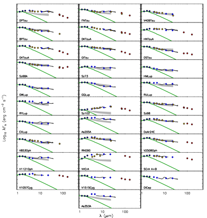
Figure 15: Same as Fig. 14, but for full disks.

Ratios of lines that trace the same kinematic component can be used to constrain the properties of the emitting gas. Simon et al. (2016) have already shown that the [O I] $\lambda$6300 and [O I] $\lambda$5577 lines have very similar LVC profiles (e.g., their Figure 15 and best fit parameters in Table 5). Section 4.1 will illustrate that, within a specific kinematic component, the similarity extends to the [S II] $\lambda$4068 line. Hence, here we use the ratios of these three forbidden lines to test if different kinematic components separate out and, if so, further refine our preliminary classification.

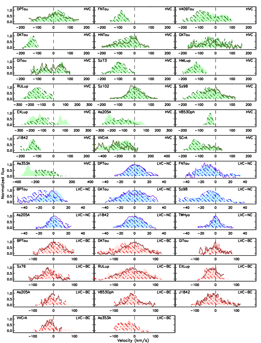
Figure 5: Comparison of the HVC (green), LVC-NC (blue), and LVC-BC (red) profiles for the [S II] $\lambda$4068 (dash-dotted line shaded area), [O I] $\lambda$5577 (solid line), and [O I] $\lambda$6300 (color filled area). Most individual kinematic components have similar profiles in the three different forbidden lines investigated here.

Figure 4 shows line ratios (left panel) or upper limits (right panel) for all 45 sources that are detected in the [O I] $\lambda$6300, the brightest of our forbidden lines. HVCs (green circles) have a combination of higher [S II] $\lambda$4068/[O I] $\lambda$6300 (hereafter SII40/OI63) and lower [O I] $\lambda$5577/[O I] $\lambda$6300  (hereafter OI55/63) ratios than LVCs. This is best illustrated by the mean and standard deviation of different component line ratios which are shown as dotted-line ellipses in both panels. Note that these values are computed from our preliminary classification and only from sources with at least two detected forbidden lines which are used to calculate line ratios.

The left panel of Fig. 4 reveals 4 possible LVCs with line ratios more compatible with HVCs (circles surrounded by green squares: one LVC-BC from DP Tau (ID 1) and HN TauA (ID 8), and one LVC-NC and one LVC-BC from Sz 102 (ID 25). Interestingly, HN TauA and Sz 102 have close to edge-on disks ($i>70^{o}$). Thus, it is very likely that, due to projection effects, their HVCs have centroids $<$30  km s^-1 and have been erroneously categorized as LVCs by our preliminary classification scheme. Although the disk inclination of DP Tau is not known, the star is about an order of magnitude underluminous compared to other Taurus members of the same spectral type (Herczeg & Hillenbrand, 2014), pointing to obscuration from a highly inclined disk (see discussions on such underluminous young stars in Fang et al. 2009, 2013b). In addition, the [O I] $\lambda$6300 and [S II] $\lambda$4068  LVC-BC centroids are close to our 30  km s^-1 HVC/LVC boundary. Thus, we re-classify all these four LVCs as HVCs, see last column of Table 2.

Fig. 4 also shows the expected SII40/OI63 and OI55/63 ratios for gas at 10⁴ K where collisions with electrons (densities $10^{5.8-8.5}$ cm^-3) excite the upper level of the transitions (e.g., Natta et al. 2014 but also Sect.  4.2.1). Most HVCs have SII40/OI63 ratios higher than the model predicted ones, while most LVCs have lower ratios. We also note that one LVC-BC from As 353A (ID 48, right panel) shows higher SII40/OI63 ratios than the model predicted ones, similar to HVCs. This, combined with possible Fe I contamination in the [S II] $\lambda$4068 transition (see Appendix E), leads us to mark the LVC-BC as suspicious, last column of Table 2.

Following this refined classification, we find that 51% (23/45) of the sources with [O I] $\lambda$6300 detection have an HVC while 84% (38/45) show an LVC. Furthermore, 31% (14/45) of the sample presents an LVC-BC while 33% (15/45) has an LVC-NC. Finally, only 20% (9/45) of our sources have both LVC-BC and LVC-NC components.

Table 3: Mean line ratios and standard deviations after HVC reclassification.

Line ratios	LVC-NC	LVC-BC	HVC
Log OI55/63	$-$0.81$\pm$0.19	$-$0.62$\pm$0.20	$-$0.97$\pm$0.31
Log SII40/OI63	$-$0.56$\pm$0.35	$-$0.25$\pm$0.18	$-$0.08$\pm$0.36

Table 4: Results from the Gehan’s generalized Wilcoxon test

Log OI55/63		Log SII40/OI63
Pairs	Probability	Paris	Probability
LVC-NC/LVC-BC	p=$6\times 10^{-3}$	LVC-NC/LVC-BC	p=$1\times 10^{-2}$
LVC-NC/HVC	p=$1\times 10^{-1}$	LVC-NC/HVC	p<$5\times 10^{-5}$
LVC-BC/HVC	p$<5\times 10^{-5}$	LVC-BC/HVC	p$=4\times 10^{-4}$

4 Thermal [O I] emission and associated gas properties

4.1 The similarity of [S II] and [O I] profiles of individual kinematic components

Figure 5 shows a comparison of HVC, LVC-NC and LVC-BC profiles for the sources that are detected both in [S II] $\lambda$4068 and [O I] $\lambda$6300. Whenever detected, [O I] $\lambda$5577 lines are also superimposed. To test how similar are the profiles of individual kinematic components, we remove from the observed profile the other components using our best fit parameters reported in Table 2.

Regardless of kinematic component (HVC, LVC-BC or NC), most profiles are similar in the [O I] and [S II] lines. Only BP Tau has an LVC-NC that is clearly more blueshifted in the [S II] $\lambda$4068 than in the [O I] lines, although the line widths are actually similar. This similarity is strengthened when comparing the centroids and FWHMs of individual components (see Fig. 22 and 23 in Appendix F). Thus, we conclude that, within a kinematic component, the three lines trace a similar region. This means that their line ratios can be used to constrain the properties of the emitting gas, in particular temperature and density.

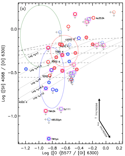
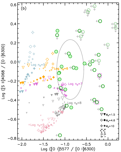
Figure 6: SII40/OI63 vs OI55/63 line ratios for LVC-NC (blue) and LVC-BC (red) in Panel (a) and HVC (green) in Panel (b). In each panel, the filled circles mark sources with detections in all three forbidden lines, thick-line open ones for those with detections in two forbidden lines, and thin-line ones for sources that have only an [O I] $\lambda$6300 detection. Magenta squares mark TDs. Dotted-line ellipses encircle the mean $\pm$ standard deviation of the HVCs (green), LVC-BCs (red), and LVC-NCs (blue) after the refined classification (see Sect.  3.4). In Panel (a), observed line ratios are compared with those predicted by thermally excited gas. Dashed grey lines locate gas at temperatures from 4,000 K (bottom) to 10,000 K (top) while dotted lines at different electron densities from $Log~{}n_{\rm e}$ (cm^-3)=6.5 (left) to $Log~{}n_{\rm e}$ (cm^-3)=10 (right). In panel (b) HVC line ratios are compared with those predicted by shock models (Hartigan & Wright, 2015). Open symbols are for $X_{e}$=0.6 while filled ones for $X_{e}$=0.1, triangles are for $M_{\rm A}$=1.5, diamonds are for $M_{\rm A}$=4.6 while stars are for a higher Mach number of 10. Different colors indicate different preshock number densities of nucleons with $Log~{}n_{0}({\rm cm^{-3}})$ from 5 to 9. Finally, the size of the symbols scales with the shock velocity ($V_{\rm s}$) which ranges from 30 to 80  km s^-1 in these models.

4.2 Gas properties constrained by line ratios

The difference in the HVC and LVC forbidden line ratios was already noted in Sect.  3.4 and used to improve upon our preliminary kinematic classification. Here, we search for and quantify any difference in line ratios between LVC-NC, LVC-BC, and HVC. Table 3 lists the mean and standard deviation of Log OI55/63 and Log SII40/OI63 for three types of components when considering only detections. LVC-BCs have the largest mean Log OI55/63 ratio while HVCs have the lowest one. HVCs have the highest mean Log SII40/OI63 ratio while LVC-NCs the lowest one.

Next, we include upper limits and use the Gehan’s generalized Wilcoxon test in the ASURV code (Feigelson & Nelson, 1985) to quantify any statistically significant difference between pairs of kinematic components. The test finds a low probability that the HVC Log OI55/63 and Log SII40/OI63 are the same as the LVC-BC. HVC and LVC-NC also have statistically different Log SII40/OI63, but indistinguishable Log OI55/63. Finally, the LVC-BC and NC differ both in Log OI55/63 ratios and Log SII40/OI63, see Table 4. These findings suggest that the combination of these three forbidden lines is sufficient to separate the kinematic components discussed in this paper.

4.2.1 Thermally excited gas explains most LVC line ratios

Figure 6 (a) shows the relation between the SII40/OI63 and the OI55/63 ratios for the LVC components. In the same figure we also plot predicted ratios for homogeneous and isothermal gas that is thermally excited by collisions with electrons (grey lines). When computing these ratios we take the solar sulfur abundance, $\alpha({\rm S})=1.4\times 10^{-5}$ (Asplund et al., 2005), and a depleted oxygen abundance as in the interstellar medium, $\alpha({\rm O})=3.2\times 10^{-4}$ (Savage & Sembach, 1996). Following Natta et al. (2014), we also assume that all oxygen is neutral while all sulfur is singly ionized. Gas at higher temperature and electron density is predicted to have higher SII40/OI63 and OI55/63 line ratios.

Most of the observed LVC ratios correspond to thermally excited gas with temperatures between 5,000 and 10,000 K and electron densities$\sim 10^{7}-10^{8}$ cm^-3. In As 353A, its LVC-BC have SII40/OI63 ratio higher than expected from this simple model, with a value seen in some of the HVC. As discussed in Sect.  3.4, the [S II] $\lambda$4068 line in this very high accretion rate star is blended with Fe I emission and classified as suspicious in Table 2, after our attempt at deblending. Turning to the LVC NC, three of the transition disk sources, TW Hya, TWA 3A, and Sz 111, have much lower SII40/OI63 ratios than those expected for gas at $\sim$5,000 K. The Gehan’s generalized Wilcoxon test finds a low probability (p= $6\times 10^{-2}$) that the SII40/OI63 ratios of LVC-BCs of full disks and TDs are drawn from the same parent population while their OI53/63 ratios are indistinguishable (p=0.3 for both the LVC NC and BC). This can be explained if TDs have a decreased S II over O I abundance ratio, as could happen if sulfur is sequestered in large grains in the disk midplane.

4.2.2 Shock-heated gas explains most HVC line ratios

Jets generate shock waves in the surrounding medium where part of their kinetic energy is converted into thermal motion, thereby producing bright forbidden line emission (e.g., Giannini et al. 2015). To further investigate the origin of the HVCs detected in our sample we compare their [S II] and [O I] line ratios to those expected from the shock models of Hartigan & Wright (2015), see Fig. 6 (b). The model line ratios were calculated for a range of input parameters: $Log~{}n_{0}({\rm cm^{-3}})=2-11$ with an increment of unity in log scale, $X_{e}$=0.1 and 0.6, $V_{\rm s}$=30–80 km s^-1, $M_{\rm A}$=1.5, 4.6 and 10. Here, $n_{0}$ is the preshock number density of nucleons, $X_{e}$ is the preshock ionization fraction, $V_{\rm S}$ is the shock velocity, and $M_{\rm A}$ is the Alfvénic Mach number. We have also scaled the ratios to the atomic abundances used in Sect. 4.2.1, $\alpha({\rm O})=3.2\times 10^{-4}$ and $\alpha({\rm S})=1.4\times 10^{-5}$, from the original solar abundances in Hartigan & Wright (2015).

Shock models with a pre-shock number density of $Log~{}n_{0}({\rm cm^{-3}})\sim 6-7$ can reproduce most of the observed SII40/OI63 and OI55/63 HVC line ratios. As forbidden line emission occurs in the post-shock cooling zone, the specific transition critical density and excitation temperature dictates how close to the front the emitting material is located. For instance the [O I] $\lambda$6300 line probes gas slightly closer to the front than the [S II] $\lambda$6731(see e.g., Figure 3 in Hartigan & Wright 2015), which has a similar excitation temperature but a critical density about hundred times lower. The [S II] $\lambda$4068 line investigated in this work has similar temperature and density to the [O I] $\lambda$6300, hence should also trace denser/hotter gas closer to the front than the [S II] $\lambda$6731.

5 Mass outflow to mass accretion rate

5.1 Mass accretion rates

After flux-calibrating our spectra (see Appendix B), we estimate the accretion luminosity using 12 emission lines covered by the HIRES spectra, including five Balmer lines (H$\zeta$, H$\delta$, H$\gamma$, H$\beta$, and H$\alpha$), four He I line (4026, 4471, 5876, and 6678Å), the He II line at 4686Å, and the Ca II lines at 3934 and 3968 Å. These lines are chosen because their luminosities are known to correlate tightly with accretion luminosities (e.g., Herczeg & Hillenbrand 2008; Fang et al. 2009; Rigliaco et al. 2012; Alcalá et al. 2014, 2017). After computing line luminosities we convert them into accretion luminosities via the empirical relations listed in Appendix G. Table 5 lists the accretion luminosities derived from the transitions discussed above as well as the 3$\sigma$-clipping mean of the accretion luminosities for each source. Mean accretion luminosities are converted into mass accretion rates using the following relation:

$$\dot{M}_{\rm acc}=\frac{L_{{\rm acc}}R_{\star}}{{\rm G}M_{\star}(1-\frac{R_{\star}}{R_{\rm in}})},$$ (1)

where $R_{\rm in}$ denotes the truncation radius of the disk, which is taken to be 5 $R_{\star}$ (Gullbring et al., 1998), G is the gravitational constant, $M_{\star}$ is the stellar mass, and $R_{\star}$ is the stellar radius. Mass accretion rates are also listed in Table 5. Our sample covers a large range in accretion luminosities and mass accretion rates, from Log($L_{\rm acc}/L_{\odot}$)=$-$3.48 to 0.72 and Log$(\dot{M}_{acc}/M$_⊙ yr^-1)=$-$10.15 to $-$6.12, estimated from the accretion-related emission lines.

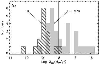
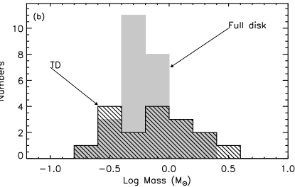
Figure 7: Panel (a): Distribution of accretion rates for full disks (grey-color filled histogram) and TDs (hatch-filled histogram). The solid line and the dashed line mark the median accretion rates of full disks and TDs, respectively. Panel (b): Distribution of stellar masses for full disks (grey-color filled histogram) and TDs (hatch-filled histogram).

We do not detect any accretion-related emission lines from DoAr 21 ($\lambda$=4420–6300 Å), DoAr 24E ($\lambda$=4420–6300 Å), SR 21A ($\lambda$=3650–6300 Å), and V1057 Cyg ($\lambda$=3650–6300 Å), hence we do not list their accretion rates in Table 5. Note that V1057 Cyg and V1515 Cyg are well known FU Ori objects. For this class of objects accretion luminosities are best derived from the emission of their self-luminous disks (e.g., Kenyon et al. 1998) and we use the more recent estimates from Green et al. (2006) in our paper. Interestingly, the spectra of DoAr 21 and DoAr 24E do not show any [O I] $\lambda$6300 emission while that of SR 21A only a marginal detection, see Appendix C for more details. To clarify which sources are truly accreting, we also compare the derived accretion luminosities with typical chromospheric values (see Manara et al. 2017). Only TWA 3A has an accretion luminosity below the chromospheric emission, suggesting that chromospheric activity dominates the line emission.

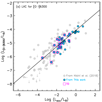
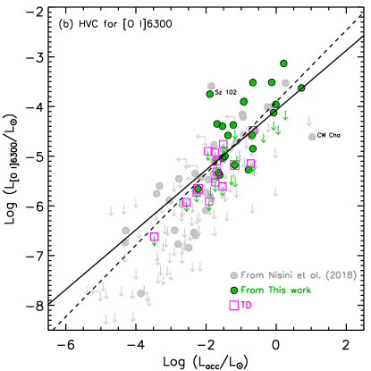
Figure 8: Line luminosities for the [O I] $\lambda$6300 LVC (Panel a) and for the HVC (Panel b) vs accretion luminosities. Magenta squares mark TDs, color-filled circles are sources from this work, while gray circles are additional sources from Nisini et al. (2018). Solid lines are the best linear fit to all LVC detections present in Panel (a). The additional dashed line in Panel (b) gives the best fit linear relation to the detected HVCs. The upper limits in Panel  (b) for our sample are calculated assuming a Gaussian profile with the FWHM of 70 km s^-1, a median of the HVC FWHM, and a peak of 3$\times rms$

Figure 7(a) compares the distribution of accretion rates for full disks (gray filled histogram) and TDs (hatch-filled histogram). The K-S test returns a low probability (P$\sim 1.8\times 10^{-5}$) for the full disks and TDs to be drawn from the same parent population. The accretion rates of TDs are systematically lower than those of full disks with a median value of 1.6$\times 10^{-9}$ $M_{\odot}$yr^-1, about seven time lower than that of the full disks in our sample. A similar result is reported in Najita et al. (2015) when comparing full and transition disks in Ophiuchus and Taurus. Fig. 7(b) compares the distribution of stellar masses. The K-S test gives a 55% probability that the two samples are drawn from the same stellar mass distribution, hence the difference in accretion rates most likely relates to their different evolutionary stage.

5.2 Correlation between [O I] and accretion luminosity

Previous work has shown that the [O I] $\lambda$6300  line luminosity correlates with stellar properties like stellar and accretion luminosity but not with X-ray luminosity (e.g., Rigliaco et al. 2013 and Nisini et al. 2018). Here, we repeat the analysis by combining our sample with that of Nisini et al. (2018), as they cover a large range in stellar properties, and by implementing the new Gaia distances (Bailer-Jones et al., 2018) for all samples. Our goal is to clarify which correlations are present and provide the most up-to-date relations with accurate distances for individual sources.

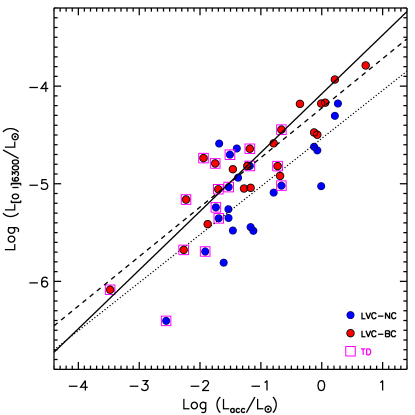
Figure 9: Line luminosities for [O I] $\lambda$6300 LVC-NC (blue) and LVC-BC (red) vs accretion luminosities. Magenta squares mark TDs. The solid line is the linear fit to the total LVC (see Fig. 8, Panel (a)), while the dashed line and dotted line are the best fits to the LVC-BC and LVC-NC, respectively.

Figure 8 (a, b) shows the relationship between the LVC (NC+BC) and HVC [O I] $\lambda$6300  line luminosity versus the accretion luminosity. The Spearman’s rank correlation coefficients for the LVCs and HVCs are 0.79 and 0.55, respectively, with a probability lower than $5\times 10^{-5}$ that the data are uncorrelated. We perform outlier-resistant two-variable linear regressions including only the detections and obtain the following relationships:

$$Log~{}L_{\rm OI63,LVC}=(0.60\pm 0.03)Log~{}L_{\rm acc}-(4.07\pm 0.06)$$ (2)

$$Log~{}L_{\rm OI63,HVC}=(0.72\pm 0.07)Log~{}L_{\rm acc}-(3.90\pm 0.11)$$ (3)

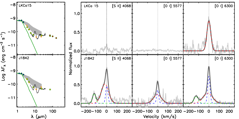
Figure 10: Left panels: SEDs of two TDs, LkCa 15 and J1842, around stars of similar spectral type and accretion rate. In each panel, the grey region show the upper and lower quartiles of the Lynds 1641 classical T Tauri median SED with the same spectral type. The median SED has been reddened with the extinction of each source, and then normalized to the J-band flux. Right panels: [S II] $\lambda$4068, [O I] $\lambda$5577, and [O I] $\lambda$6300 line profiles from the same sources. While these systems have very similar SEDs, the forbidden line profiles suggest that the inner gaseous disk of LkCa 15 is in a more evolved stage than that of J1842.

The slope for the $L_{\rm OI63,LVC}$ vs. $L_{\rm acc}$ in this work is similar to those (0.52$\pm$0.07, 0.59$\pm$0.04) in Rigliaco et al. (2013) and Nisini et al. (2018), but much flatter than the one (0.81$\pm$0.09) in Natta et al. (2014), which could be due to their smaller sample size. Our $L_{\rm OI63,HVC}$ vs. $L_{\rm acc}$ slope is also similar to the one (0.75$\pm$0.08) in Nisini et al. (2018), but slightly flatter than the one ($\sim$0.9) in Rigliaco et al. (2013). The $L_{\rm OI63,HVC}$ vs. $L_{\rm acc}$ slope is steeper than the $L_{\rm OI63,LVC}$ vs. $L_{\rm acc}$ slope with a 2$\sigma$ confidence, consistent with the findings in Rigliaco et al. (2013). Note that using only our sources we find the same slopes as those reported in Equations 2 and  3 within the, now larger, uncertainties (0.60$\pm$0.06 and 0.62$\pm$0.16).

For our sources we can further correlate the line luminosity of individual LVC components with $L_{\rm acc}$, see Figure 9. The Pearson correlation coefficients for the LVC-NC and LVC-BC are 0.71 and 0.92 with two-sided p-values of 1.4$\times$10^-4 and 7.6$\times$10^-10, respectively. This means that their luminosities are correlated with the accretion luminosity with the LVC-BC displaying a higher correlation than the NC and the total LVC (see Fig. 8(a)). The outlier-resistant two-variable linear regression gives the following relations:

$$Log~{}L_{\rm OI63,LVC-BC}=(0.51\pm 0.05)Log~{}L_{\rm acc}-(4.22\pm 0.07)$$ (4)

$$Log~{}L_{\rm OI63,LVC-NC}=(0.49\pm 0.10)Log~{}L_{\rm acc}-(4.53\pm 0.14)$$ (5)

The $L_{\rm OI63,LVC-BC}$ and the $L_{\rm OI63,LVC-NC}$ vs. $L_{\rm acc}$ slopes are the same within the uncertainties.

5.3 Inner disk evolution traced by the [O I] emission

The evolutionary stage of a star+disk system is often assessed from its SED. However, optical forbidden lines can aid in understanding the evolutionary stage of a system by probing the evolution of the gas content (see e.g., Figure 5 in Ercolano & Pascucci 2017).

The frequency of different [O I] $\lambda$6300 line components differ for full and TDs, see Table 6 where we provide statistics for our sample. Full disks more frequently than TDs show an HVC in their [O I] $\lambda$6300 profiles, and a BC accompanied by an NC. In contrast, TDs more frequently than full disks present only a LVC-NC or BC. In addition, TDs have simpler line profiles: $\sim$81% (13/16) of our TDs only show one LVC-NC or one LVC-BC without any other LVC or HVCs components, while this fraction is down to 24% (7/29) for the full disks, see also Figures 16 and 17 in Appendix A. With a larger sample of 65 T Tauri stars, Banzatti et al. (2018) also find that those surrounded by a TD tend to show only a single component in their [O I] $\lambda$6300 line profile (see their Section 5.5 for details). The much lower fraction of TDs with an HVC and a BC+NC with respect to full disks might indicate an evolution in disk winds (see also Ercolano & Pascucci 2017). The TDs in our sample have lower mass accretion rates than full disks, hence lower HVC and LVC luminosities (Figure 8), and likely a more depleted inner gas disk. As also suggested in Banzatti et al. (2018), winds in TDs might be launched from larger radii, have a larger opening angle, and not re-collimate into jets.

Table 6: Statistics on the line profiles

	Only NC	Only BC	NC+BC	HVC
Full disks	28% (8/29)	24% (7/29)	24% (7/29)	72% (21/29)
TDs	44% (7/16)	44% (7/16)	13% (2/16)	13% (2/16)

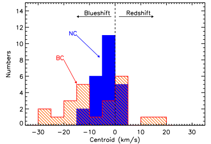
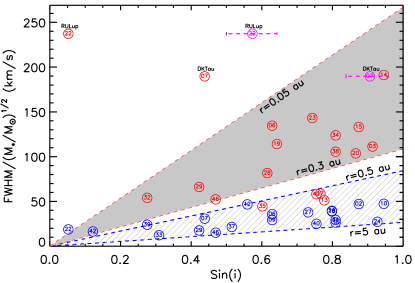
Figure 11: Upper panel: Distribution of centroids for the LVC-NC (blue-color filled histogram) and the LVC-BC (hatch-filled histogram). Note that many centroids are blueshifted with respect to the stellar velocity (see also Banzatti et al. 2018 for more details on the [O I] kinematics). Bottom panel: FWHM corrected for instrumental broadening and normalized by the stellar mass vs disk inclination, LVC-BC in red and LVC-NC in blue. Dashed lines show Keplerian FWHM as a function of disk inclination at radii of 0.05, 0.3, 0.5, and 5 au. The hatch-filled area and grey color-filled area enclose most of the NC and BC, respectively. The magenta circles locate two sources (RU Lup, ID 22, and DK TauA, ID 7) for which we also use alternative disk inclinations.

Furthermore, the [O I] $\lambda$6300 line profiles can be used to distinguish the evolutionary stage of systems with similar SEDs. An example is shown in Figure 10 for LkCa 15 and J1842, both classified as TDs. The central stars have similar spectral types (K5.5 vs. K3) and accretion rates ($1.8\times 10^{-9}$ vs. $3.0\times 10^{-9}$ $M_{\odot}~{}yr^{-1}$ ), and their disks present very similar SEDs. However, their forbidden line profiles are clearly different: LkCa 15 only presents a LVC-BC (with a FWHM, 44.6  km s^-1, near the boundary to separate the LVC NCs and BCs) in the [O I] $\lambda$6300, while J1842 shows a LVC-NC, a LVC-BC, and a HVC in both the [S II] $\lambda$4068 and [O I] $\lambda$6300  lines, and a LVC-NC and a LVC-BC in the [O I] $\lambda$5577 line. Thus, while both sources would appear to be in the same evolutionary stage based on their SED, the forbidden line profiles demonstrate that the inner gaseous disk of LkCa 15 is in a more evolved stage than that of J1842.

5.4 Mass outflow rates

Previous analysis of [O I] $\lambda$6300 high-resolution spectra has demonstrated that a significant number of LVC-BC and NC peak centroids are blueshifted with respect to the stellar velocity (Simon et al. 2016; McGinnis et al. 2018; Banzatti et al. 2018). With the largest blueshifts found in sources surrounded by lower inclination disks and an emitting region within $\sim$0.5 au from the star, Simon et al. (2016) attributed the LVC-BC to the base of an MHD-driven wind. Although the focus of our paper is on forbidden line luminosities and line ratios, here we show that the kinematics of the LVC-BC and NC of our sample are consistent with previous findings.

The upper panel of Fig. 11 shows the distribution of the NC and BC centroids. About 63% (15/24) of NCs and 52% (12/23) of BCs have blueshifts larger than 1.5  km s^-1, while only 8% (2/24) of NCs and 9% (5/23) of BCs are redshifted. The larger proportion of blueshifts when compared to no shift or redshifts is consistent with a wind origin for both components. The lower panel of Fig. 11 shows the relation between disk inclination and the BC and NC FWHMs, corrected for instrumental broadening and normalized by stellar mass.

If we attribute the line width primarily to Keplerian broadening as in previous studies (Simon et al., 2016; McGinnis et al., 2018), most BCs trace radii within 0.5 au while NCs probe gas further out but mostly within $\sim$5 au. A few sources appear as outliers in this plot and are worth discussing. First, the FWHM from DK TauA and RU Lup are much larger than those expected from pure Keplerian rotation using the disk inclinations given in Table 1. The disk inclination of DK TauA is not well constrained: the 20^∘ value we adopted here comes from the analysis of mm CO lines but the continuum emission points to a much higher inclination of 65^∘ (Simon et al., 2017). In the case of RU Lup the outer disk inclination of $3^{\circ}$ derived from ALMA mm imagery may not apply to the forbidden lines studied here. Indeed, spectroastrometry in the CO rovibrational band suggests a higher inclination of 35^∘ for the inner disk (Pontoppidan et al., 2011) and an even higher inclination is implied by MIDI visibilities (see Varga et al. 2018 and Banzatti et al. 2018 for further details). If we use these alternative/higher disk inclinations, the BC FWHM of DK TauA falls in the same region as the other BCs and that of RU Lup becomes much closer to that region. Finally, the BCs from LkCa 15, Sz 73, RNO 90, and VV CrA fall within the domain of LVC-NC, they could have been misclassified using our stringent cut in FWHM that does not take into account disk inclination.

Having established that our sample supports the scenario in which LVC-BC and NC trace a wind and their FWHMs are consistent with being broadened by Keplerian rotation, we use the [O I] $\lambda$6300 luminosity and our constraints on the gas temperature, velocity, and emitting radii to compute wind mass loss rates. Fig. 6(a) shows that electron densities $n_{e}\geq 3\times 10^{6}$ cm^-3 are needed to reproduce the measured LVC line ratios. As these densities are larger than the [O I] $\lambda$6300 critical density, which is $1.8\times 10^{6}$ cm^-3, the LVC emitting gas is most likely in LTE. In addition, very high densities are required to make the [O I] $\lambda$6300 line optically thick (see Table 9 in Hollenbach & McKee 1989). Hence, we will use equations for optically thin LTE gas to relate the LVC [O I] $\lambda$6300 luminosity to a gas mass. As a shock origin is more likely for the HVC emission and this lower density gas may not be in LTE, see Sect.  4.2.2 and Fig. 6 (b), we will use equations derived for radiative shocks to estimate the mass loss rate from this high-velocity component.

5.4.1 Mass loss rates from the LVC

As the [O I] $\lambda$6300 line is optically thin its luminosity ($L_{6300}$) can be written as:

$$L_{6300}=N_{\rm u}~{}A~{}h\nu$$ (6)

Where $N_{\rm u}$ is the total number of O atoms in the upper ${}^{1}D_{2}$ level, $A$ is the transition probability (6.503$\times 10^{-3}$), and $h\nu$ is the associated energy they emit (Dere et al., 1997). In addition, for gas in LTE the total number of O atoms ($N$) is related to $N_{\rm u}$ as:

$$N_{\rm u}=N~{}\frac{g_{u}~{}e^{-h\nu/kT}}{Z(T)}$$ (7)

Where the $g_{u}$ is the upper level statistical weight, $k$ is the Boltzmann constant, $T$ is the gas temperature, and $Z(T)$ is the partition function at temperature $T$. We calculate $Z(T)$ assuming a 5-level oxygen atom. Considering that in disks the abundance of neutral oxygen is reduced because half of the cosmic O is in silicate grains (Jenkins, 2009) and the wind is launched from outside the dust sublimation radius (Fig. 11 lower panel), we take $\alpha({\rm O})$=3.2$\times$10^-4 to calculate the total mass of gas $M$ from the total number of O I atoms. Finally, the mass loss rate $\dot{M}_{\rm wind}$ can be written as:

$$\dot{M}_{\rm wind}=M\frac{V_{\rm wind}}{l_{\rm wind}}$$ (8)

Where $V_{\rm wind}$ and $l_{\rm wind}$ are the velocity and wind height. We further write the unconstrained wind height as $l_{\rm wind}=f\times r_{\rm base}$, i.e. the wind vertical extent is $f$ times the emitting radius at the base of the wind. Combining Equations 6 through to  8, we have:

$$\dot{M}_{\rm wind}= \frac{V_{\rm wind}}{l_{\rm wind}}\frac{\eta m_{\rm H}}{\alpha({\rm O})}~{}e^{h\nu/kT}{Z(T)}\frac{L_{6300}}{g_{\rm u}~{}A~{}h\nu}$$ (9)

$$={\rm C(T)}\Big{(}\frac{V_{\rm wind}}{10~{}{\rm km~{}s^{-1}}}\Big{)}\Big{(}\frac{l_{\rm wind}}{1~{}{\rm au}}\Big{)}^{-1}\Big{(}\frac{L_{6300}}{L_{\odot}}\Big{)}M_{\odot}～yr^{-1}$$

Where $\eta$=1.34 is the ratio of total gas mass to Hydrogen mass. From this equation it is clear that the estimated mass loss rate has a strong dependence on the gas temperature $T$ and scales linearly with $V_{\rm wind}$ and $l_{\rm wind}$. LVC gas temperatures range from 5,000 to 10,000 K (Sect.  4.2.1) and within this range $C(T)$ varies by an order of magnitude: from 2.4$\times$10^-4 for $T$=5,000 K down to 2.6$\times$10^-5 for $T$=10,000 K.

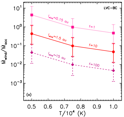
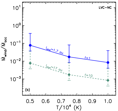
Figure 12: Median $\dot{M}_{\rm wind}$/$\dot{M}_{\rm acc}$ ratios for our sample as a function of gas temperature and for different wind heights ($l_{\rm wind}=f\times r_{\rm base}$), LVC-BC left panel and LVC-NC right panel. In each panel, the error bars show the upper and lower quartiles of the $\dot{M}_{\rm wind}$/$\dot{M}_{\rm acc}$ ratio distributions.

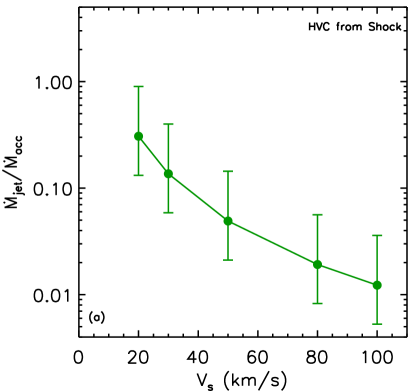
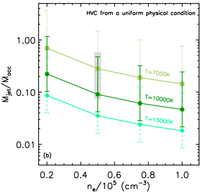
Figure 13: Left panel: Median $\dot{M}_{\rm jet}$/$\dot{M}_{\rm acc}$ ratio as a function of shock velocity assuming that HVC arises in post-shock gas. Right panel: Median $\dot{M}_{\rm jet}$/$\dot{M}_{\rm acc}$ as a function of electron density and for different gas temperatures assuming that HVC are produced in uniform physical conditions. Error bars show the upper and lower quartiles of the median $\dot{M}_{\rm jet}$/$\dot{M}_{\rm acc}$ ratios for our sample while the grey region for sources in Nisini et al. (2018) which are reported in their paper only for $T$=10,000 K, $n_{\rm e}$=$5\times 10^{4}$ cm^-3.

For each source with an [O I] $\lambda$6300 detection we calculate its own $\dot{M}_{\rm wind}$ by taking as $V_{\rm wind}$ the median of projected peak velocities and as $r_{\rm base}$ the Keplerian radius from half of the line FWHM, corrected for the instrumental broadening and projected (see Fig. 11 lower panel). For the BC these values correspond to $-$15  km s^-1 and 0.15 au while for the NC they are $-$6  km s^-1 and 1.7 au. We then divide $\dot{M}_{\rm wind}$ by each source $\dot{M}_{\rm acc}$ and show in Figure 12 (panels a and b) how the median and upper and lower quartile ratios depend on $T$ and $l_{\rm wind}$. As expected from Equation 9, $\dot{M}_{\rm wind}$, and hence $\dot{M}_{\rm wind}/\dot{M}_{\rm acc}$ ratios, increase with decreasing gas temperature and wind height. Since the extent of the [O I] $\lambda$6300 emitting region is unknown, we vary the factor $f$ within a range of plausible values for which $l_{\rm wind}$ is similar in the LVC-BC and NC.

For the BC, $f=1$ produces unreasonably large $\dot{M}_{\rm wind}/\dot{M}_{\rm acc}$ ratios for most temperatures, except for 10,000 K. However, such a high temperature is unlikely otherwise emission lines from ionized oxygen would have been also easily detected (see Sect. 5.7 in Simon et al. 2016). Heating processes not driven by photons (e.g., ambipolar drift heating, see Safier 1993) could result in higher gas temperatures without affecting the ionization state, but their efficiency has not been sufficiently explored in this context. We will further discuss the implications of Fig. 12 in Sect.  6. However, it is already worth noting that, for likely wind extents, the mass loss rates implied by the BC are much higher than those implied by the NC. This results from the fact that [O I] $\lambda$6300 luminosities as well as the median peak centroid are larger for the LVC-BC than for the NC component (see Figs. 9 and 11) and the wind heights of the NC are likely higher than for the BC.

This last point is important, hence we summarize here additional arguments supporting a large vertical extent of the LVC-NC. First, it is highly unlikely that the wind height of the LVC-NC is small (f$<$1) compared to the Keplerian radius because with our high-resolution ($\Delta$v$\sim$6km/s) spectra we would see double peaked NC profiles. Next, as we will discuss, it is very likely that the extent of the NC is larger than that of the BC. The LVC-BC traces an MHD wind because of its small Keplerian radius (0.05–0.5 au) and blueshifted centroids; thermal pressure is insufficient to launch the gas flow and MHD forces are required. The NC may similarly also trace an MHD wind. In both cases the wind is not expected to extend much beyond the Alfvén surface since the magnetic field cannot hold the gas in rigid rotation and the wind will be accelerated and collimated into jets beyond the Alfvén surface (Blandford & Payne, 1982). In MHD simulations, the height of the Alfvén surface above the disk surface is about 0.5–1.5 the wind launching radius (Pudritz et al., 2006; Bai, 2017). Since the NC is launched further out (1–5 au), its vertical extent is therefore likely to be larger than that of the BC. If the LVC-NC is partly supported by a photoevaporative (thermal) wind, it should be even more extended vertically given the gas temperature (5,000–10,000K) inferred from the line ratios (see Fig. 6). As an example, in the X-ray-driven photoevaporative wind model (Ercolano & Owen, 2016), the winds can extend to about 35 au above the disk. While the wind height cannot be determined without spatially resolved observations, our finding that the mass loss rates implied by the BC are higher than those implied by the NC should be reliable.

5.4.2 Mass loss rates from the HVC

As discussed in Section 4.2.2 shock models reproduce most of the [OI] and [SII] HVC line ratios. In fast shocks, most of the mechanical energy of the preshock gas is converted into heat (e.g. Shull & McKee 1979, Hollenbach & McKee 1979). The mass loss rate can then be estimated assuming that a certain fraction of the kinetic energy is radiated away in the [O I] $\lambda$6300 line. Hence, we use the equations for radiative shocks as presented e.g. in Hollenbach & Gorti (2009). If the hydrogen density is high ($n_{\rm H}\sim 10^{6}$ cm^-3), the line luminosity can be computed as:

$$L_{6300}=\frac{y_{0}}{2}\dot{M}_{\rm loss}V_{\rm s}^{2}$$ (10)

With $y_{0}$ being to the fraction of cooling that goes into the [O I] $\lambda$6300 line and $V_{\rm s}$ the shock velocity. The mass-loss rate is then:

$$\dot{M}_{\rm jet}=L_{6300}\frac{2}{y_{0}}V_{\rm s}^{-2}$$ (11)

At a density $n_{\rm H}\sim 10^{6}$ cm^-3, $y_{0}$ is around 0.1-0.3, hence we take here $y_{0}=0.2$. As for the LVC, we first compute individual $\dot{M}_{\rm jet}$ divide them by each source $\dot{M}_{\rm acc}$ and show the behavior of median, upper and lower quartile ratios for a range of shock velocities compatible with observations (e.g., Hartigan et al. 1987). The faster the shock velocity the lower the $\dot{M}_{\rm jet}$/$\dot{M}_{\rm acc}$ ratio. For a typical shock velocity of 30  km s^-1 (Hartigan et al., 1994), the median $\dot{M}_{\rm jet}$/$\dot{M}_{\rm acc}$ ratio is around 0.1.

The approach we have taken above differs from the one typically used in the literature where it is assumed that the jet has uniform properties within the slit width and the line luminosity is calculated from a collisional excitation model akin to that described in Section 4.2.1 for the LVC (see also Fig. 6 left panel). More specifically and following Hartigan et al. (1995) and Nisini et al. (2018), the mass loss rate from the jet can be written as:

$$\dot{M}_{\rm jet}={\rm C(T,n_{\rm e})}\Big{(}\frac{V_{\perp}}{100~{}{\rm km~{}s^{-1}}}\Big{)}\Big{(}\frac{l_{\perp}}{100~{}{\rm au}}\Big{)}^{-1}\Big{(}\frac{L_{6300}}{L_{\odot}}\Big{)}M_{\odot}～yr^{-1}$$ (12)

Where $V_{\perp}$ is the component of the jet velocity in the plane of the sky (we assume 100  km s^-1 as Nisini et al. 2018) and $l_{\perp}$ is the projected size of the slit aperture (0$\farcs$861) on the plane of the sky. C(T, $n_{\rm e}$) depends on the gas temperature and electron density and is calculated assuming a 5-level oxygen atom as in Section 4.2.1. For $T$=10,000 K, $C(T,n_{\rm e})$ are 9.0$\times$10^-5, 6.1$\times$10^-5, and 4.6$\times$10^-5 for $n_{\rm e}=5.0\times 10^{4}$, 7.5$\times 10^{4}$ and $1.0\times 10^{5}~{}{\rm cm^{-3}}$, respectively. Taking the same temperature (10,000 K) and electron density ($5.0\times 10^{4}$ cm^-3) as Nisini et al. (2018), we find a median $\dot{M}_{\rm jet}$/$\dot{M}_{\rm acc}$ ratio of $\sim$0.1. The right panel of Fig. 13 also shows the $\dot{M}_{\rm jet}$/$\dot{M}_{\rm acc}$ for the [O I] $\lambda$6300 detected HVCs in Nisini et al. (2018) after implementing the new Gaia distances (Bailer-Jones et al., 2018) and assuming $\alpha({\rm O})=3.2\times 10^{-4}$, T=10,000 K, and $n_{\rm e}=5.0\times 10^{4}$ cm^-3. The median $\dot{M}_{\rm jet}$/$\dot{M}_{\rm acc}$ ratio is $\sim$0.18 for this sample . Furthermore, the same panel shows the dependence of $\dot{M}_{\rm jet}$/$\dot{M}_{\rm acc}$ on $T$ and $n_{\rm e}$: the ratio decreases with increasing gas temperature and electron density. For values of $T$$\sim$7,000–15,000 K and $n_{\rm e}$=$2-6\times 10^{4}$ cm^-3 that are appropriate for the base of the T Tauri jets (Hartigan & Morse, 2007; Agra-Amboage et al., 2011; Giannini et al., 2013; Maurri et al., 2014), the median $\dot{M}_{\rm jet}$/$\dot{M}_{\rm acc}$ ratios vary from 0.8 to 0.04.

6 Discussion

It is already well established that the HVC and the LVC components of forbidden lines trace different physical environments, where the HVC is more spatially extended and formed in shock-excited collimated jets, and the LVC, with a higher density than the HVC, is confined to scales of less than 5 AU (e.g., Hartigan et al. 1995, Hirth et al. 1997, Simon et al. 2016). Our study expands upon the literature by combining the [S II] $\lambda$4068 transition with the well-studied [O I] $\lambda$6300 and [O I] $\lambda$5577 lines, demonstrating that the same kinematic components appear in all 3 lines, thus enabling the use of component line ratios to constrain the properties of the emitting gas (Sect.  4.1 and Fig. 5). By including detections and upper limits we found that the HVC SII40/OI63 ratios are statistically higher than the LVC (both BC and NC) and that there is a low probability that the BC OI55/63 ratios are drawn from the same parent population as the NC and HVC (Table 4). These differences and the mean line ratios of the three components corroborate previous suggestions, mostly based on kinematics (e.g., Simon et al. 2016, McGinnis et al. 2018, Banzatti et al. 2018), that the LVC-BC traces a higher density/hotter region than the LVC-NC, probably the base of an MHD disk wind. Finally, we could show that thermally excited gas with temperatures 5,000$-$10,000 K and electron densities $\sim 10^{7}-10^{8}$ cm^-3 can explain most of the LVC-BC and NC line ratios while the HVC ratios are best reproduced by radiative shock models where forbidden lines arise in the hot ($\sim$7,000$-$10,000 K) but less dense (total H density $\sim 10^{6}$ cm^-3) post-shock cooling zone (Sect.  4.2.1 and  4.2.2).

Armed with the physical properties of the emitting gas in each component, we computed mass loss rates for the LVC-BC, NC, and HVC (Sect.  5.4). To evaluate the efficiency of winds in removing disk mass we also computed mass accretion rates by converting the luminosity of several permitted lines covered in our spectra to the accretion luminosity (Sect.  5.1). For the HVC, we relied on radiative shock models that convert a fraction of the mechanical energy of the pre-shock gas into the [O I] $\lambda$6300 luminosity. We found relatively low $\dot{M}_{\rm jet}/\dot{M}_{\rm acc}$ with a median value $\sim$0.1 for typical shock velocities of 30  km s^-1, but this ratio could be as low as 0.01 for a high shock velocity of 100  km s^-1 or as high as 0.3 for a low shock velocity of 20  km s^-1. These values are similar to those previously reported in the literature, which were instead calculated assuming a collisional excitation model, and hence sensitive to several not well constrained quantities such as gas temperature and electron density in addition to jet velocity (e.g., Hartigan et al. 1995, Nisini et al. 2018, and Sect.  5.4.2).

A first estimate for mass loss rates for the LVC, assuming a spherical outflow geometry, comes from Natta et al. (2014) who find $\dot{M}_{\rm wind}/\dot{M}_{\rm acc}$ between 0.1 and 1 for their sample of T Tauri stars in Lupus and $\sigma$ Ori. These values are on the high end of the HVC $\dot{M}_{\rm jet}/\dot{M}_{\rm acc}$ ratios, suggesting that the LVC may have a higher mass loss rate than the jet. Our work is the first to provide $\dot{M}_{\rm wind}/\dot{M}_{\rm acc}$ separately for the BC and NC. One important finding is that the mass loss rate from the BC exceeds that from the NC by at least a factor of 5. A comparison of the mass loss rates between the BC and HVC is more uncertain. To this end we explored the sensitivity of wind mass loss rates in thermally excited gas to the parameters that are the least constrained and most affect the estimates, namely the gas temperature and $l_{\rm wind}$ (Sect.  5.4.1). For the BC, a wind extent equal to the radial extent inferred from Keplerian broadening of the [O I] $\lambda$6300 lines ($f=1$ Fig. 12 left panel) provides unreasonably large $\dot{M}_{\rm wind}/\dot{M}_{\rm acc}$, i.e. larger than 1, for most sources. Most likely the vertical extent of the BC, which remains unconstrained from our data, is larger than the Keplerian radius inferred from the BC FWHM. If we assume a vertical extent comparable to the NC radius inferred from Keplerian broadening ($f=1$ Fig. 12 right panel and $f=10$ Fig. 12 left panel) the median $\dot{M}_{\rm wind}/\dot{M}_{\rm acc}$ from the BC ranges from $\sim$0.05 for gas as hot as 10,000 K up to $\sim$0.4 for gas at 5,000 K. As already discussed in Sect.  5.4.1, a temperature of 10,000 K is unlikely for the LVC gas, hence higher mass loss rates are more realistic. However, given the sensitivity of $\dot{M}_{\rm wind}/\dot{M}_{\rm acc}$ on $l_{\rm wind}$ we cannot conclusively state that the LVC-BC is carrying away more mass than the HVC. What is more certain is that the NC $\dot{M}_{\rm wind}/\dot{M}_{\rm acc}$ is lower than the BC for reasonable $l_{\rm winds}$ by at least a factor of 5. Thus, most of the disk mass appears to be lost close to the central star in the region traced by the BC.

How do our results compare with theoretical models of winds? Both photoevaporative and MHD winds have been proposed to explain forbidden line emission. However, as already pointed out by Simon et al. (2016) and confirmed by McGinnis et al. (2018) and Banzatti et al. (2018), the only component that may be tracing a thermal photoevaporative wind is the LVC-NC, as the BC is formed well inside the gravitational potential well of the star. Our finding that most NC ratios can be reproduced by thermally excited gas and that the line luminosity correlates with accretion luminosity agree with the most recent predictions from X-ray-driven photoevaporative winds (Ercolano & Owen, 2016). In these models, stellar EUV photons heat the forbidden line emitting region and, due to their low penetration depth, constrain it to a thin vertically extended (up to $\sim$35 au) zone above the inner disk (see e.g. their Fig. 4). In addition, Ercolano & Owen (2016) claim that most of EUV luminosity comes from accretion and that would lead to a correlation between the [OI] luminosity and $L_{\rm acc}$. The vertical extent of the emitting region results in a wide range of wind velocities that can broaden the [OI] lines up to $\sim$30  km s^-1  for close to edge-on disks while keeping moderate blueshifts of up to $\sim$7  km s^-1  for disks inclined by $\sim 50^{\circ}$ with respect to the observer. While the predicted FWHM and peak centroids are consistent with most of the LVC-NC values we report here, more detailed kinematic comparisons disfavor a thermal outflow origin because several [O I] $\lambda$6300 widths are still larger than predicted (McGinnis et al. 2018, Banzatti et al. 2018), the largest observed blueshifts occur for a lower disk inclination than predicted, and the centroids of the BC and NC are correlated (see Banzatti et al. 2018 for further details). For these reasons we favor a similar origin for both the BC and the NC in an MHD wind.

MHD wind models come in two broad categories: (1) winds arising close to the co-rotation radius ($\leq$0.1 au), such as X-winds (e.g., Shang et al. 2007), conical winds (e.g., Romanova et al. 2009), magnetospheric ejections (e.g., Zanni & Ferreira 2009) or accretion powered stellar winds (e.g., Matt & Pudritz 2005) and (2) winds arising over a broad range of radii in the disk, from 0.1 to 10 au, sometimes called D-winds (e.g., Pudritz et al. 2007). A key difference between these two genres of models is that the former are important in removing angular momentum from the accreting star, enabling it to spin down, and the latter in removing angular momentum from the disk itself, enabling accretion to occur through the disk rather than relying on some kind of magnetic viscosity (e.g., MRI). Note that these types of winds are not mutually exclusive. All of these scenarios can reproduce the terminal velocity of the fast ($\sim 100$  km s^-1) outflowing gas traced by the HVC. However, only D-winds can account for the high angular resolution observations showing a decrease in outflow velocity with increasing jet radius, implying an "onion-like" layering of a faster flow engirdled by a slower flow (e.g., Bacciotti et al. 2000, 2002, Pyo et al. 2002, 2003, Takami et al. 2004, Beck et al. 2010, Agra-Amboage et al. 2011). Also D-winds provide a natural explanation for possible rotation signatures in jets, implying wind footpoints spanning a large range of disk radii, from $\sim$0.1 to 5 au (e.g., Ferreira et al. 2006, Cabrit 2009).

Our results provide strong support for the presence of D-winds, although they do not help in determining whether D-winds are the dominant contributor to the jet traced by the HVC, or whether the jet is primarily fed by an MHD wind from near the co-rotation radius. However, the Keplerian radii for the BC infered from their FWHM are larger than the co-rotation radii ($\sim$0.05 au), and the ones for NCs are well beyond the co-rotation radii, implying a large range of wind radii (from $\sim$0.05 out to 5 au), similar to those expected in D-winds and inferred from jet rotation signatures. The observed correlation between the [O I] line and accretion luminosity might indicate that the wind truly drives accretion: as the [O I] $\lambda$6300 line is optically thin a higher luminosity implies more mass removed in the wind, and hence more angular momentum promoting mass accretion from the disk onto the central star.

Another prediction from some D-wind models is that most of the mass is lost within a few au from the central star (e.g., Pelletier & Pudritz 1992), in agreement with our finding that the BC has larger $\dot{M}_{\rm wind}/\dot{M}_{\rm acc}$ than the NC. This last result also places interesting constraints on more recent disk simulations that include non-ideal MHD effects (e.g., Bai 2014, Gressel et al. 2015, Béthune et al. 2017 ). These simulations show that disk winds are launched from radii extending out to $\sim 10-20$ au with vigorous mass loss rates out to these radii (see also Bai 2017). However, even for gas at 5,000 K we obtain an $\dot{M}_{\rm wind}/\dot{M}_{\rm acc}$ of 0.4 from the upper quartile of the $f=1$ LVC-NC curve (Fig. 12 right panel) suggesting that the mass loss rate is not as large as predicted out to the $\sim$5 au radii we can trace with the NC. If the theoretically predicted winds exist, most of the gas must be cooler ($<5,000$K) than what can be traced with the forbidden lines analyzed here. Other wind diagnostics that can probe cooler neutral hydrogen in the flow would be valuable in determining the presence of more extended disk winds.

7 Summary

We analyzed optical high-resolution spectra, covering the [S II] $\lambda$4068, [O I] $\lambda$5577, and [O I] $\lambda$6300 forbidden lines, from a sample of 48 T Tauri stars, 31 of which are surrounded by full disks while 17 by TDs. We detected the [O I] $\lambda$6300  from 45 sources, the [O I] $\lambda$5577  from 26 sources, and the [S II] $\lambda$4068  from 22 sources. Following Simon et al. (2016), we decomposed the line profiles into HVC, LVC-NC, and LVC-BC. As in previous studies, we attribute the line width primarily to Keplerian broadening, with forbidden emission arising both in the inner (BC within 0.5 au) and outer (NC within 1$-$5 au) disk. Many components show peak centroids blueshifted by more than 1.5  km s^-1  with respect to the stellar velocity. Thus, the LVC is most likely tracing unbound slow wind gas. After flux calibrating our spectra we derived line luminosity and line ratios for individual kinematic components to assess the properties of the emitting gas and with the goal of measuring mass loss rates. We also estimated mass accretion rates using 12 accretion-related permitted lines to then evaluate the mass loss over mass accretion rate. Our main results can be summarized as follows:

1. About 72% of full disks present a HVC, while this number is down to 13% for TDs. Furthermore, TDs more frequently than full disks show only a LVC-NC (44% for TDs vs. 28% for the full disks), while full disks tend to show line profiles with multiple components. These findings point to a depletion of gas in the inner disk of TDs, in agreement with their lower average mass accretion rate.

2. The HVC and LVC [O I] $\lambda$6300 luminosity is confirmed to correlate with the accretion luminosity. When the [O I] $\lambda$6300 LVC is decomposed into LVC-BC and NC, we see that the LVC-BC luminosity is more tightly correlated with accretion luminosity than the NC.

3. The profiles of individual kinematic components are similar in the [S II] $\lambda$4068, [O I] $\lambda$5577, and [O I] $\lambda$6300 lines, when detected. This indicates that they trace a similar region, hence their line ratios can be used to infer the physical properties of the emitting gas.

4. The HVC has statistically different SII40/OI63 ratios than the LVC-BC and NC. Its OI55/63 ratios are also statistically different from the LVC-BC, while they are not distinguishable from the LVC-NC. These differences and the mean line ratios corroborate previous suggestions that the BC traces hot/dense gas close to the base of an MHD wind.

5. Most LVC-BC and NC ratios can be explained by thermally excited gas with electron densities of $\sim 10^{7}-10^{8}$ cm^-3 and temperatures 5,000$-$10,000 K. HVC line ratios are better explained by shock models with a pre-shock number density of nucleons of $\sim 10^{6}-10^{7}$cm^-3.

6. Building on the [O I] $\lambda$6300 HVC luminosity, converting a fraction of the shock mechanical energy into radiant energy, and adopting a typical shock velocity of 30  km s^-1, we find a median $\dot{M}_{\rm jet}$/$\dot{M}_{\rm acc}$ ratio of 0.1. This value is comparable to previous results from the literature which were calculated with a very different approach. The agreement between these different approaches to convert HVC luminosity into a mass outflow rate suggests this ratio may be robust. An $\dot{M}_{\rm jet}$/$\dot{M}_{\rm acc}$ of 0.1 reflects a minimal impact on disk mass removal by outflowing material seen in the jet.

7. Building on our finding that the [OI] LVC emission is most likely thermal, gas is in LTE, and the [O I] $\lambda$6300 line is optically thin, we estimate for the first time $\dot{M}_{\rm wind}$/$\dot{M}_{\rm acc}$ ratios separately for the BC and NC. We show that $\dot{M}_{\rm wind}$ is a factor of 5 higher in the BC (inner disk) than the NC (outer disk). However absolute $\dot{M}_{\rm wind}$ values are sensitive to the gas temperature and wind height, making direct comparisons between outflow rates in the LVC and the HVC uncertain. However, for plausible wind heights, we find that the mass flowing out in the BC is likely at least as large as in the HVC and may be considerably higher. If so, then the inner disk wind traced by the BC may play an important role in the evolution of the disk mass.

Taken together our results favor D-wind models. In particular, we find that winds are launched from a range of disk radii beyond the gas co-rotation radius even in the LVC-BC alone. In addition, most of the mass is lost close to the star, within a few au. For plausible wind heights, LVC-NC $\dot{M}_{\rm wind}$/$\dot{M}_{\rm acc}$ ratios are lower than $\sim 0.4$, and thus lower than the ratios predicted by recent non-ideal MHD simulations for radii $\sim 1-20$ au (e.g. Bai 2017). Additional wind diagnostics tracing cooler gas would be helpful to test if indeed radially extended winds could drive accretion.

Table 2: Parameters for line decomposition of [S II] $\lambda$4068, [O I] $\lambda$5577, and [O I] $\lambda$6300 line profiles

		[S II] $\lambda$4068				[O I] $\lambda$5577				[O I] $\lambda$6300
		$FWHM$	$v_{\rm c}$	$EW$	Log $L_{\rm 4069}$	$FWHM$	$v_{\rm c}$	$EW$	Log $L_{\rm 5577}$	$FWHM$	$v_{\rm c}$	$EW$	Log $L_{\rm 6300}$	preliminary	refined
ID	Name	( km s-1)	( km s-1)	(Å)	($L_{\odot}$)	( km s-1)	( km s-1)	(Å)	($L_{\odot}$)	( km s-1)	( km s-1)	(Å)	($L_{\odot}$)	Class	Class
1	DPTau	62.8	$-91.9$	1.01	$-5.29$	45.4	$-90.6$	0.08	$-6.32$	64.4	$-89.3$	0.89	$-5.24$	HVC-B
		115.6	$31.2$	5.92	$-4.52$	116.7	$13.6$	0.47	$-5.54$	111.8	$23.5$	6.03	$-4.41$	LVC-BC	HVC-R
		27.3	$2.4$	1.23	$-5.20$	24.4	$0.4$	0.60	$-5.44$	22.5	$0.8$	3.99	$-4.59$	LVC-NC
2	CXTau	$\cdots$	$\cdots$	$\cdots$	$\cdots$	$\cdots$	$\cdots$	$\cdots$	$<-6.52$	27.9	$-2.6$	0.05	$-6.40$	LVC-NC
3	FPTau	$\cdots$	$\cdots$	$\cdots$	$<-5.51$	84.6	$1.4$	0.14	$-6.14$	66.0	$1.1$	0.38	$-5.68$	LVC-BC
4	FNTau	13.8	$-44.1$	0.09	$-6.18$	$\cdots$	$\cdots$	$\cdots$	$<-6.47$	10.6	$-43.0$	0.03	$-6.25$	HVC-B
		15.3	$-117.8$	0.14	$-5.99$	$\cdots$	$\cdots$	$\cdots$	$<-6.36$	13.7	$-121.6$	0.06	$-6.00$	HVC-B
		40.5	$-79.2$	0.95	$-5.17$	$\cdots$	$\cdots$	$\cdots$	$<-5.91$	38.3	$-77.4$	0.47	$-5.11$	HVC-B
		30.4	$-11.1$	0.27	$-5.72$	22.8	$-12.3$	0.02	$-6.45$	26.9	$-12.2$	0.34	$-5.26$	LVC-NC
5	V409Tau	113.3	$-85.4$	0.92	$-5.58$	$\cdots$	$\cdots$	$\cdots$	$<-5.81$	107.6	$-64.8$	0.22	$-5.50$	HVC-B
		70.8	$42.5$	0.29	$-6.08$	$\cdots$	$\cdots$	$\cdots$	$<-5.95$	79.3	$51.5$	0.10	$-5.83$	HVC-R
6	BPTau	94.7	$11.3$	0.36	$-5.22$	88.3	$4.0$	0.17	$-5.24$	98.9	$12.4$	0.26	$-5.04$	LVC-BC
		37.5	$-18.2$	0.11	$-5.73$	27.5	$-6.1$	0.03	$-6.01$	26.3	$-2.6$	0.10	$-5.44$	LVC-NC
7	DKTau	45.1	$-125.6$	0.16	$-5.30$	$\cdots$	$\cdots$	$\cdots$	$<-5.69$	41.0	$-135.7$	0.09	$-5.27$	HVC-B
		124.2	$-18.1$	0.29	$-5.05$	96.8	$-1.4$	0.16	$-5.02$	153.7	$-27.4$	0.42	$-4.59$	LVC-BC
		$\cdots$	$\cdots$	$\cdots$	$<-5.79$	14.2	$1.0$	0.02	$-5.88$	24.9	$-5.1$	0.13	$-5.09$	LVC-NC
8	HNTau	116.2	$-78.5$	2.80	$-4.25$	183.1	$-57.9$	0.23	$-5.19$	132.4	$-67.7$	2.99	$-4.07$	HVC-B
		60.2	$-9.6$	1.44	$-4.54$	45.3	$-0.0$	0.10	$-5.56$	50.4	$-6.5$	1.33	$-4.42$	LVC-BC	HVC-B
9	UXTau	$\cdots$	$\cdots$	$\cdots$	$<-5.20$	$\cdots$	$\cdots$	$\cdots$	$<-5.18$	34.6	$-1.2$	0.11	$-4.70$	LVC-NC
10	GKTau	160.6	$-22.4$	0.36	$-4.87$	116.6	$-35.5$	0.04	$-5.57$	179.1	$-30.7$	0.38	$-4.58$	HVC-B
		36.0	$-1.0$	0.13	$-5.31$	51.5	$3.1$	0.05	$-5.48$	38.6	$-3.3$	0.17	$-4.94$	LVC-NC
11	GITau	86.3	$-51.9$	0.20	$-4.79$	38.9	$-52.6$	0.03	$-5.73$	85.9	$-67.5$	0.19	$-4.85$	HVC-B
		33.6	$46.3$	0.15	$-4.91$	54.1	$40.6$	0.05	$-5.44$	31.7	$46.7$	0.17	$-4.90$	HVC-R
		39.3	$6.2$	0.08	$-5.20$	59.0	$-11.5$	0.06	$-5.38$	44.7	$1.3$	0.16	$-4.92$	LVC-BC
12	DMTau	$\cdots$	$\cdots$	$\cdots$	$<-6.17$	24.8	$-2.0$	0.05	$-6.51$	26.1	$0.5$	0.35	$-5.69$	LVC-NC
13	LKCa15	$\cdots$	$\cdots$	$\cdots$	$<-5.47$	$\cdots$	$\cdots$	$\cdots$	$<-5.54$	44.6	$-0.6$	0.14	$-5.06$	LVC-BC
14	DSTau	$\cdots$	$\cdots$	$\cdots$	$<-4.86$	$\cdots$	$\cdots$	$\cdots$	$<-4.93$	151.1	$16.3$	0.19	$-5.05$	LVC-BC
15	Sz65A	$\cdots$	$\cdots$	$\cdots$	$<-4.92$	$\cdots$	$\cdots$	$\cdots$	$<-4.87$	109.9	$3.6$	0.25	$-4.74$	LVC-BC
16	Sz68A	$\cdots$	$\cdots$	$\cdots$	$<-6.55$	$\cdots$	$\cdots$	$\cdots$	$<-5.49$	$\cdots$	$\cdots$	$\cdots$	$<-5.50$	$\cdots$	$\cdots$
17	Sz73	82.5	$-88.4$	0.70	$-4.89$	$\cdots$	$\cdots$	$\cdots$	$<-5.39$	71.1	$-94.4$	1.67	$-4.43$	HVC-B
		$\cdots$	$\cdots$	$\cdots$	$<-5.09$	$\cdots$	$\cdots$	$\cdots$	$<-5.27$	94.2	$64.2$	0.25	$-5.26$	HVC-R
		$\cdots$	$\cdots$	$\cdots$	$<-5.35$	41.1	$-11.9$	0.11	$-5.66$	50.8	$-19.2$	0.69	$-4.82$	LVC-BC
18	HMLup	68.3	$-119.7$	0.50	$-5.78$	$\cdots$	$\cdots$	$\cdots$	$<-5.70$	90.4	$-116.9$	0.59	$-5.38$	HVC-B
		$\cdots$	$\cdots$	$\cdots$	$<-6.41$	$\cdots$	$\cdots$	$\cdots$	$<-6.31$	22.1	$-3.8$	0.22	$-5.81$	LVC-NC
19	GWLup	$\cdots$	$\cdots$	$\cdots$	$<-5.99$	68.8	$-7.5$	0.09	$-5.93$	69.4	$-9.7$	0.29	$-5.41$	LVC-BC
20	GQLup	$\cdots$	$\cdots$	$\cdots$	$<-4.56$	46.1	$10.7$	0.04	$-5.04$	91.4	$4.0$	0.28	$-4.18$	LVC-BC
21	Sz76	$\cdots$	$\cdots$	$\cdots$	$<-5.80$	69.9	$31.7$	0.22	$-5.86$	50.1	$38.8$	0.39	$-5.66$	HVC-R
		77.9	$-16.0$	0.48	$-5.64$	53.1	$-26.4$	0.24	$-5.81$	65.5	$-18.3$	1.21	$-5.16$	LVC-BC
22	RULup	130.0	$-137.8$	1.68	$-3.68$	$\cdots$	$\cdots$	$\cdots$	$<-4.67$	109.9	$-149.3$	0.61	$-4.01$	HVC-B
		68.5	$-38.9$	0.26	$-4.49$	$\cdots$	$\cdots$	$\cdots$	$<-5.10$	40.5	$-32.3$	0.07	$-4.92$	HVC-B
		150.3	$-13.1$	0.43	$-4.28$	120.5	$-11.7$	0.21	$-4.47$	176.4	$-10.1$	0.41	$-4.18$	LVC-BC
		$\cdots$	$\cdots$	$\cdots$	$<-5.21$	$\cdots$	$\cdots$	$\cdots$	$<-5.57$	13.9	$-10.9$	0.06	$-5.02$	LVC-NC
23	IMLup	$\cdots$	$\cdots$	$\cdots$	$<-4.98$	$\cdots$	$\cdots$	$\cdots$	$<-4.83$	117.1	$-10.0$	0.16	$-4.79$	LVC-BC
24	RYLup	$\cdots$	$\cdots$	$\cdots$	$<-5.18$	$\cdots$	$\cdots$	$\cdots$	$<-5.13$	30.7	$2.5$	0.09	$-4.64$	LVC-NC
25	Sz102	206.1	$-32.5$	20.69	$-4.54$	$\cdots$	$\cdots$	$\cdots$	$<-5.54$	209.3	$-38.1$	22.13	$-4.63$	HVC-B
		58.3	$-25.8$	17.62	$-4.61$	30.7	$-16.0$	0.89	$-5.92$	40.0	$-24.5$	17.99	$-4.72$	LVC-NC	HVC-B
		85.3	$20.6$	53.70	$-4.13$	108.9	$5.9$	4.45	$-5.22$	93.6	$11.8$	127.33	$-3.87$	LVC-BC	HVC-R

Table 2: Parameters for line decomposition of [S II] $\lambda$4068, [O I] $\lambda$5577, and [O I] $\lambda$6300 line profiles

		[S II] $\lambda$4068				[O I] $\lambda$5577				[O I] $\lambda$6300
		$FWHM$	$v_{\rm c}$	$EW$	Log $L_{\rm 4069}$	$FWHM$	$v_{\rm c}$	$EW$	Log $L_{\rm 5577}$	$FWHM$	$v_{\rm c}$	$EW$	Log $L_{\rm 6300}$	preliminary	refined
ID	Name	( km s-1)	( km s-1)	(Å)	($L_{\odot}$)	( km s-1)	( km s-1)	(Å)	($L_{\odot}$)	( km s-1)	( km s-1)	(Å)	($L_{\odot}$)	Class	Class
26	Sz111	$\cdots$	$\cdots$	$\cdots$	$<-6.16$	$\cdots$	$\cdots$	$\cdots$	$<-5.91$	28.0	$-0.4$	0.41	$-5.24$	LVC-NC
27	Sz98	167.4	$-50.9$	2.05	$-4.46$	108.9	$-12.4$	0.21	$-5.13$	152.5	$-37.7$	1.07	$-4.40$	HVC-B
		30.4	$-8.1$	0.21	$-5.46$	$\cdots$	$\cdots$	$\cdots$	$<-5.75$	28.7	$-6.7$	0.12	$-5.35$	LVC-NC
28	EXLup	$\cdots$	$\cdots$	$\cdots$	$\cdots$	$\cdots$	$\cdots$	$\cdots$	$<-4.98$	25.1	$-119.3$	0.08	$-4.53$	HVC-B
		84.3	$-181.2$	0.17	$-3.86$	$\cdots$	$\cdots$	$\cdots$	$<-4.48$	79.6	$-179.2$	0.26	$-4.03$	HVC-Ba
		121.9	$-88.0$	0.81	$-3.19$	$\cdots$	$\cdots$	$\cdots$	$<-4.69$	48.9	$-79.5$	0.14	$-4.29$	HVC-B
		$\cdots$	$\cdots$	$\cdots$	$\cdots$	$\cdots$	$\cdots$	$\cdots$	$<-4.88$	31.5	$102.8$	0.06	$-4.64$	HVC-R
		$\cdots$	$\cdots$	$\cdots$	$\cdots$	$\cdots$	$\cdots$	$\cdots$	$<-4.88$	31.1	$56.9$	0.11	$-4.41$	HVC-R
		37.8	$-15.0$	0.10	$-4.11$	65.1	$-15.8$	0.07	$-4.53$	59.6	$-17.6$	0.45	$-3.79$	LVC-BC
29	As205A	$\cdots$	$\cdots$	$\cdots$	$\cdots$	$\cdots$	$\cdots$	$\cdots$	$<-5.09$	56.3	$-221.9$	0.11	$-4.69$	HVC-B
		154.2	$-112.1$	0.29	$-4.29$	$\cdots$	$\cdots$	$\cdots$	$<-4.49$	225.5	$-85.4$	0.28	$-4.27$	HVC-Ba
		60.4	$-19.0$	0.12	$-4.67$	50.8	$-0.7$	0.03	$-5.18$	54.5	$-13.5$	0.16	$-4.50$	LVC-BC
		18.9	$1.5$	0.03	$-5.36$	12.7	$1.1$	0.02	$-5.40$	14.5	$-0.7$	0.11	$-4.66$	LVC-NC
30	DoAr21	$\cdots$	$\cdots$	$\cdots$	$\cdots$	$\cdots$	$\cdots$	$\cdots$	$<-4.31$	$\cdots$	$\cdots$	$\cdots$	$<-4.51$	$\cdots$
31	DoAr24E	$\cdots$	$\cdots$	$\cdots$	$\cdots$	$\cdots$	$\cdots$	$\cdots$	$<-5.69$	$\cdots$	$\cdots$	$\cdots$	$<-5.62$	$\cdots$
32	DoAr44	$\cdots$	$\cdots$	$\cdots$	$<-5.04$	35.0	$3.8$	0.02	$-5.68$	59.6	$-1.1$	0.15	$-4.82$	LVC-BC
33	SR21A	$\cdots$	$\cdots$	$\cdots$	$<-3.29$	$\cdots$	$\cdots$	$\cdots$	$<-4.45$	16.3	$-6.9$	0.01	$-4.81$	LVC-NC
34	V853Oph	30.0	$-33.8$	1.26	$-5.27$	$\cdots$	$\cdots$	$\cdots$	$<-6.10$	28.5	$-31.3$	0.93	$-5.00$	HVC-B
		68.4	$-16.0$	1.19	$-5.30$	37.5	$-12.4$	0.24	$-5.62$	70.2	$-14.4$	1.31	$-4.85$	LVC-BC
		$\cdots$	$\cdots$	$\cdots$	$<-6.52$	$\cdots$	$\cdots$	$\cdots$	$<-6.33$	16.6	$-1.6$	0.31	$-5.48$	LVC-NC
35	RNO90	$\cdots$	$\cdots$	$\cdots$	$<-4.14$	56.1	$-3.0$	0.06	$-4.73$	57.5	$-3.4$	0.23	$-4.17$	LVC-BC
36	V2508Oph	$\cdots$	$\cdots$	$\cdots$	$<-4.49$	$\cdots$	$\cdots$	$\cdots$	$<-4.67$	116.2	$-38.4$	0.11	$-4.85$	HVC-B
37	V1121Oph	$\cdots$	$\cdots$	$\cdots$	$<-5.64$	$\cdots$	$\cdots$	$\cdots$	$<-5.54$	21.1	$-7.2$	0.03	$-5.48$	LVC-NC
38	J1842	36.5	$-122.1$	0.06	$-5.60$	$\cdots$	$\cdots$	$\cdots$	$<-5.43$	45.6	$-126.3$	0.10	$-5.18$	HVC-B
		83.9	$-16.4$	0.28	$-4.94$	93.0	$-3.1$	0.08	$-5.29$	109.2	$-11.5$	0.35	$-4.64$	LVC-BC
		25.9	$1.8$	0.08	$-5.50$	23.4	$-1.0$	0.03	$-5.71$	27.3	$-0.5$	0.23	$-4.82$	LVC-NC
39	J1852	$\cdots$	$\cdots$	$\cdots$	$<-5.86$	$\cdots$	$\cdots$	$\cdots$	$<-5.88$	23.5	$-2.4$	0.09	$-5.35$	LVC-NC
40	VVCrA	$\cdots$	$\cdots$	$\cdots$	$<-3.60$	85.2	$-416.1$	0.06	$-5.06$	133.2	$-361.6$	0.78	$-3.88$	HVC-B
		135.5	$-209.3$	1.88	$-3.52$	94.7	$-234.8$	0.30	$-4.37$	119.7	$-205.4$	1.58	$-3.57$	HVC-Ba
		147.8	$-88.8$	3.89	$-3.21$	101.5	$-78.5$	0.14	$-4.71$	114.2	$-87.0$	1.73	$-3.53$	HVC-B
		35.7	$-22.5$	0.48	$-4.11$	51.4	$-19.8$	0.18	$-4.59$	42.2	$-22.1$	0.69	$-3.93$	LVC-BC
		$\cdots$	$\cdots$	$\cdots$	$<-4.34$	$\cdots$	$\cdots$	$\cdots$	$<-4.99$	18.1	$-6.7$	0.29	$-4.30$	LVC-NC
41	SCrAA+B	44.1	$-129.3$	0.24	$-4.67$	$\cdots$	$\cdots$	$\cdots$	$<-5.02$	45.6	$-127.7$	0.51	$-3.91$	HVC-B
		132.7	$-72.3$	0.60	$-4.27$	121.1	$-40.4$	0.09	$-4.65$	128.0	$-49.5$	0.66	$-3.80$	HVC-B
		58.5	$59.1$	0.07	$-5.19$	$\cdots$	$\cdots$	$\cdots$	$<-4.85$	68.2	$68.0$	0.08	$-4.70$	HVC-R
42	TWHya	15.9	$-0.3$	0.08	$-6.29$	9.6	$0.1$	0.08	$-5.89$	12.8	$0.0$	0.57	$-5.03$	LVC-NC
43	TWA3A	$\cdots$	$\cdots$	$\cdots$	$<-7.03$	56.0	$-1.1$	0.11	$-6.98$	61.9	$1.3$	0.59	$-6.09$	LVC-BC
44	V1057Cyg	$\cdots$	$\cdots$	$\cdots$	$<-1.61$	$\cdots$	$\cdots$	$\cdots$	$<-2.51$	50.0	$-154.6$	0.23	$-1.88$	HVC-B
		$\cdots$	$\cdots$	$\cdots$	$<-1.55$	$\cdots$	$\cdots$	$\cdots$	$<-2.45$	58.0	$-98.6$	0.24	$-1.86$	HVC-B
		$\cdots$	$\cdots$	$\cdots$	$<-1.27$	$\cdots$	$\cdots$	$\cdots$	$<-2.17$	110.9	$-60.0$	0.25	$-1.85$	HVC-B
45	V1515Cyg	$\cdots$	$\cdots$	$\cdots$	$<-3.05$	$\cdots$	$\cdots$	$\cdots$	$<-3.28$	32.1	$-120.8$	0.03	$-3.45$	HVC-B
		$\cdots$	$\cdots$	$\cdots$	$<-2.72$	$\cdots$	$\cdots$	$\cdots$	$<-2.94$	69.9	$-63.2$	0.18	$-2.73$	HVC-B
46	HD143006	$\cdots$	$\cdots$	$\cdots$	$<-4.37$	$\cdots$	$\cdots$	$\cdots$	$<-4.73$	66.3	$2.8$	0.09	$-4.45$	LVC-BC
		$\cdots$	$\cdots$	$\cdots$	$<-4.91$	$\cdots$	$\cdots$	$\cdots$	$<-5.27$	19.1	$2.1$	0.02	$-5.02$	LVC-NC
47	DICep	$\cdots$	$\cdots$	$\cdots$	$<-4.75$	$\cdots$	$\cdots$	$\cdots$	$<-4.69$	27.3	$-7.5$	0.11	$-4.18$	LVC-NC
48	As353A	$\cdots$	$\cdots$	$\cdots$	$\cdots$	$\cdots$	$\cdots$	$\cdots$	$<-4.77$	48.4	$-280.0$	0.21	$-4.25$	HVC-B
		318.0	$-128.6$	1.96	$-3.67$	$\cdots$	$\cdots$	$\cdots$	$<-3.96$	322.8	$-126.6$	0.94	$-3.61$	HVC-Ba
		95.1	$-43.2$	0.41	$-4.35$	$\cdots$	$\cdots$	$\cdots$	$<-4.66$	62.7	$-27.9$	0.13	$-4.47$	LVC-BC	Suspicious
		$\cdots$	$\cdots$	$\cdots$	$\cdots$	$\cdots$	$\cdots$	$\cdots$	$<-4.99$	29.1	$-4.2$	0.09	$-4.62$	LVC-NC

^a The fitted parameters for the components from [S II] $\lambda$4068 are unreliable.

Table 5: The accretion luminosity and accretion rates of the sources in this work

		Log $L_{\rm acc}$
		(H$\zeta$)	(H$\delta$)	(H$\gamma$)	(H$\beta$)	(H$\alpha$)	(He I $\lambda$4026)	(He I $\lambda$4471)	(He I $\lambda$5876)	(He I $\lambda$6678)	(He II $\lambda$4686)	(Ca II $\lambda$3934)	(Ca II $\lambda$3968)	Log $\overline{L_{\rm acc}}$	Log $\dot{M}_{acc}$
ID	Name	($L_{\odot}$)	($L_{\odot}$)	($L_{\odot}$)	($L_{\odot}$)	($L_{\odot}$)	($L_{\odot}$)	($L_{\odot}$)	($L_{\odot}$)	($L_{\odot}$)	($L_{\odot}$)	($L_{\odot}$)	($L_{\odot}$)	($L_{\odot}$)	($M_{\odot}~{}yr^{-1}$)
1	DPTau	$\cdots$	$-1.74$	$-1.73$	$-1.69$	$-2.17$	$-1.74$	$-1.55$	$-1.91$	$-1.95$	$-1.87$	$-1.35$	$-1.46$	$-1.69$	$-9.07$
2	CXTau	$\cdots$	$\cdots$	$-2.44$	$-2.32$	$-2.62$	$\cdots$	$-2.66$	$-3.12$	n	n	$\cdots$	$\cdots$	$-2.56$	$-9.37$
3	FPTau	$\cdots$	$-2.32$	$-2.32$	$-2.15$	$-2.16$	$\cdots$	$-2.24$	$-2.53$	$-2.23$	$-2.31$	$\cdots$	$\cdots$	$-2.27$	$-9.17$
4	FNTau	$\cdots$	$-1.50$	$-1.47$	$-1.48$	$-1.87$	$-1.58$	$-1.44$	$-1.33$	$-1.12$	$-1.92$	$\cdots$	$\cdots$	$-1.53$	$-7.97$
5	V409Tau	$\cdots$	n	n	n	a	n	n	n	n	n	$-1.53$	$-1.79$	$-1.64$	$-8.44$
6	BPTau	$-0.99$	$-1.16$	$-1.19$	$-1.16$	$-1.24$	$-1.25$	$-1.24$	$-1.22$	$-1.18$	$-1.14$	$-1.13$	$-1.02$	$-1.17$	$-8.14$
7	DKTauA	$-0.67$	$-0.89$	$-0.87$	$-0.76$	$-1.18$	$-0.79$	$-0.98$	$-0.74$	$-0.72$	$-0.74$	$-0.76$	$-0.64$	$-0.79$	$-7.86$
8	HNTauA	$\cdots$	$-1.10$	$-1.26$	$-1.00$	$-1.92$	$-0.54$	$-0.78$	$-1.46$	$-0.85$	$-1.10$	$-0.89$	$-0.67$	$-0.93$	$-8.37$
9	UXTauA	$\cdots$	n	n	n	$-1.56$	n	n	n	n	n	$-1.16$	$-1.46$	$-1.51$	$-8.81$
10	GKTauA	$\cdots$	$-1.31$	$-1.56$	$-1.34$	$-1.64$	$-1.41$	$-1.47$	$-1.16$	n	$-1.30$	$-0.76$	$-0.88$	$-1.38$	$-8.35$
11	GITau	$\cdots$	$-0.55$	$-0.59$	$-0.89$	$-1.46$	$-0.71$	$-0.68$	$-0.78$	$-0.75$	$-0.64$	$\cdots$	$\cdots$	$-0.69$	$-7.61$
12	DMTau	$\cdots$	$-1.92$	$-1.94$	$-1.89$	$-1.92$	$-2.43$	$-1.91$	$-1.91$	$-2.33$	$-1.93$	$\cdots$	$\cdots$	$-1.92$	$-8.79$
13	LKCa15	$\cdots$	$-1.70$	$-1.88$	$-1.84$	$-1.65$	$-1.66$	$-1.78$	$-1.51$	n	$-1.22$	$\cdots$	$\cdots$	$-1.70$	$-8.75$
14	DSTau	$\cdots$	$-1.30$	$-1.20$	$-1.45$	$-1.67$	$-1.28$	$-1.39$	$-1.12$	$-0.93$	$-1.13$	$-1.76$	$-1.51$	$-1.28$	$-8.42$
15	Sz65	$-1.92$	$-1.87$	$-2.21$	a	$\cdots$	n	n	$-2.76$	$\cdots$	n	$-1.66$	$-1.88$	$-1.94$	$-8.90$
16	Sz68A	n	n	n	n	$\cdots$	n	n	n	$\cdots$	n	$-1.16$	$-1.20$	$-1.18$	$-8.13$
17	Sz73	$-1.14$	$-1.21$	$-1.29$	$-1.33$	$\cdots$	$-1.22$	$-1.30$	$-1.41$	$\cdots$	$-1.27$	$-1.16$	$-1.05$	$-1.22$	$-8.54$
18	HMLup	$-1.54$	$-1.62$	$-1.64$	$-1.43$	$\cdots$	$-1.69$	$-1.66$	$-1.52$	$\cdots$	$-1.98$	$-1.23$	$-1.29$	$-1.61$	$-8.45$
19	GWLup	$-1.61$	$-1.74$	$-1.80$	$-1.87$	$\cdots$	$-1.84$	$-1.99$	$-1.91$	$\cdots$	$-1.94$	$-1.89$	$-1.96$	$-1.87$	$-8.71$
20	GQLup	$-0.32$	$-0.49$	$-0.66$	$-0.40$	$\cdots$	$-0.53$	$-0.61$	$-0.26$	$\cdots$	$-0.51$	$-0.10$	$-0.11$	$-0.36$	$-7.39$
21	Sz76	$-1.92$	$-2.12$	$-2.16$	$-2.52$	$\cdots$	$-2.82$	$-2.82$	$-3.46$	$\cdots$	n	$-1.85$	$-2.22$	$-2.23$	$-8.96$
22	RULup	$-0.34$	$-0.16$	$0.03$	$-0.01$	$\cdots$	b	b	$0.11$	$\cdots$	$-0.32$	$0.18$	$0.13$	$-0.01$	$-6.76$
23	IMLup	$-1.68$	$-1.92$	a	a	$\cdots$	n	n	$-2.41$	$\cdots$	n	$-1.49$	$-1.72$	$-1.75$	$-8.68$
24	RYLup	n	n	n	n	$\cdots$	n	n	n	$\cdots$	n	$-1.39$	$-1.40$	$-1.40$	$-8.59$
25	Sz102	$-2.00$	$-1.92$	$-1.91$	$-1.71$	$\cdots$	$-1.81$	$-1.55$	$-2.26$	$\cdots$	$-1.91$	$-1.80$	$-1.57$	$-1.89$
26	Sz111	$-1.49$	$-1.65$	$-1.70$	$-1.86$	$\cdots$	$-1.67$	$-1.82$	$-1.87$	$\cdots$	$-1.69$	$-1.99$	$-1.89$	$-1.74$	$-8.79$
27	Sz98	$-1.39$	$-1.66$	$-1.66$	$-1.53$	$\cdots$	$-1.56$	$-1.80$	$-1.65$	$\cdots$	$-1.50$	$-1.42$	$-1.36$	$-1.53$	$-8.58$
28	EXLup	$0.39$	$0.53$	$0.79$	$0.62$	$\cdots$	b	$0.89$	$0.39$	$\cdots$	$0.19$	$0.99$	$0.99$	$0.72$	$-6.12$
29	As205A	$-0.44$	$-0.26$	$-0.20$	$-0.10$	$\cdots$	$-0.05$	$-0.39$	$0.02$	$\cdots$	$-0.30$	$0.23$	$0.20$	$-0.07$	$-6.58$
30	DoAr21	$\cdots$	$\cdots$	$\cdots$	n	$\cdots$	$\cdots$	n	n	$\cdots$	n	$\cdots$	$\cdots$
31	DoAr24E	$\cdots$	$\cdots$	$\cdots$	n	$\cdots$	$\cdots$	n	n	$\cdots$	n	$\cdots$	$\cdots$
32	DoAr44	$-0.64$	$-0.87$	$-0.91$	$-0.66$	$\cdots$	$-1.04$	$-1.30$	$-0.70$	$\cdots$	$-1.20$	$-0.42$	$-0.41$	$-0.73$	$-8.05$
33	SR21A	n	n	n	n	$\cdots$	n	n	n	$\cdots$	n	n	n
34	V853Oph	$-1.21$	$-1.43$	$-1.50$	$-1.48$	$\cdots$	$-1.41$	$-1.39$	$-1.38$	$\cdots$	$-1.43$	$-1.65$	$-1.54$	$-1.46$	$-8.08$
35	RNO90	$-0.01$	$0.13$	$-0.01$	$0.02$	$\cdots$	$0.32$	$0.12$	$0.05$	$\cdots$	n	$\cdots$	$\cdots$	$0.06$	$-7.26$
36	V2508Oph	$-0.56$	$-0.63$	$-0.70$	$-0.61$	$\cdots$	$-0.76$	$-0.89$	$-0.74$	$\cdots$	$-0.86$	$-0.56$	$-0.50$	$-0.66$	$-7.35$
37	V1121Oph	$-1.01$	$-1.39$	$-1.47$	$-1.06$	$\cdots$	$-1.35$	$-1.56$	$-1.10$	$\cdots$	$-1.00$	$-0.90$	$-0.95$	$-1.12$	$-8.30$
38	J1842	$-1.09$	$-1.34$	$-1.42$	$-1.11$	$\cdots$	$-1.33$	$-1.69$	$-1.08$	$\cdots$	$-1.18$	$-0.91$	$-1.11$	$-1.18$	$-8.52$
39	J1852	$-1.62$	$-1.83$	$-1.94$	$-1.61$	$\cdots$	$-1.82$	n	$-1.69$	$\cdots$	$-1.49$	$-1.66$	$-1.75$	$-1.69$	$-9.03$
40	VVCrA	$-0.22$	$0.24$	$0.25$	$0.12$	$\cdots$	b?	$-0.12$	$-0.65$	$\cdots$	n	$1.07$	$0.70$	$0.21$	$-6.43$
41	SCrA A+B	a	a	a	a	$\cdots$	b	$-0.75$	$0.14$	$\cdots$	$-0.59$	a	a	$-0.66$	$-7.43$
42	TWHya	$-1.43$	$-1.48$	$-1.42$	$-1.25$	$\cdots$	$-1.68$	$-1.64$	$-1.49$	$\cdots$	$-1.64$	$-1.83$	$-1.79$	$-1.53$	$-8.67$
43	TWA3A	$-3.51$	$-3.70$	$-3.54$	$-3.58$	$\cdots$	$-3.87$	$-3.84$	$-3.47$	$\cdots$	n	$-3.18$	$-3.18$	$-3.48$	$-10.15$
44	V1057Cyg	n	n	n	n	$\cdots$	n	n	n	$\cdots$	n	a	n		$\sim-$4.3
45	V1515Cyg	n	n	n	n	$\cdots$	n	n	n	$\cdots$	n	$1.09$	a		$\sim-4.5$
46	HD143006	n	n	n	$-0.68$	$\cdots$	n	n	n	$\cdots$	n	$-0.65$	b	$-0.66$	$-7.99$
47	DICep	$-0.05$	$-0.04$	$0.19$	$0.53$	$\cdots$	n	$0.04$	$0.27$	$\cdots$	$-0.24$	$0.54$	$0.45$	$0.26$	$-6.97$
48	As353A	n	a	a	a	$\cdots$	n	$0.08$	$-0.22$	$\cdots$	n	$-0.35$	a	$-0.13$	$-6.81$

Note: In the table, ’…’ marks the lines which are not covered or fully covered by the extracted spectra, ’a’ for the ones which appear as emission, but are strongly affected by the absorption due to the winds, ’n’ for those which do not clearly appear as emission lines, and ’b’ for the ones which are seriously contaminated by other nearby emission lines. ^c For the two FU Ori objects, their accretion rates are obtained from Green et al. (2006) by fitting the SEDs, assuming a central stellar mass of 1 $M_{\odot}$.

Appendix A Disk Classification and [O I] $\lambda$6300 line profiles

Fig. 14 and  15 show the SEDs of our sources. SEDs are constructed using the the Two-Micron All Sky Survey (2MASS, Skrutskie et al., 2006), the Spitzer and Herschel photometric data, the Spitzer IRS spectra, and the Wide-field Infrared Survey Explorer (WISE, Wright et al., 2010). For the sources in Taurus, their Spitzer data are collected from Luhman et al. (2010); Rebull et al. (2010), and the Herschel data are from Howard et al. (2013). For the sources in Lupus and $\rho$ Oph, the Spitzer data are from Evans et al. (2014), and the Herschel data are from Bustamante et al. (2015) and Rebollido et al. (2015), respectively. For the sources in Corona Australis, the Spitzer data are collected from Hillenbrand et al. (2008) and Dunham et al. (2015), and the Herschel data are from Sicilia-Aguilar et al. (2013). For the two sources in the TW Hya association, their Spitzer data are collected from Luhman et al. (2010), and their Herschel data from Riviere-Marichalar et al. (2013).

For each source in our sample, we construct a median SED from CTTs with similar spectral type in Lynds 1641 (Fang et al., 2009, 2013a). The age of Lynds 1641 is around 1-2 Myr (Fang et al., 2013a), which is similar to most of the sources in this work, besides the TW Hya association. In each panel of Fig. 14 and  15, we show in grey the upper and lower quartiles of the median SEDs. We classify a disk as TD if its SED is below the lower quartile of the Lynds 1641 median SED at more than two bands, and otherwise as a full disk. As Lynds 1641 lacks G and F-type stars (Fang et al., 2013a) we cannot use our approach to classify SR 21A, HD 143006, V1057 Cyg, V1515 Cyg, and DI Cep. In this case we adopt the TD classification for SR 21A and HD 143006, found in the literature (Najita et al., 2015; van der Marel et al., 2016), and consider the other three ones as full disks.

Fig. 16 and  17 show the [O I] $\lambda$6300 line profiles for the TDs and full disks. It is clear that the TDs have simpler forbidden line profiles than the full disks.

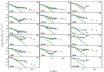
Figure 14: SEDs for the TDs analyzed in this paper. Filled circles are photometric data from 2MASS (blue), Spitzer (yellow), and Herschel (red). Open circles are used for WISE photometry. The black solid line shows the Spitzer IRS spectrum while the green solid line the stellar photosphere. The grey region shows the upper and lower quartiles of the Lynds 1641 classical T Tauri median SED. The median SED has been reddened with the extinction of each source, and then normalized to the J-band flux.

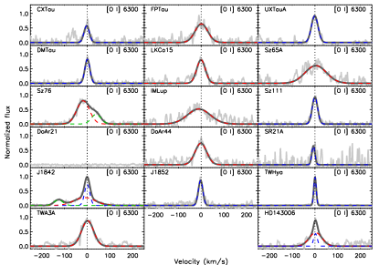
Figure 16: [O I] $\lambda$6300  line profiles for TDs. The SEDs of the corresponding sources are shown in Fig. 14.

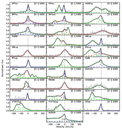
Figure 17: [O I] $\lambda$6300  line profiles for full disks. The SEDs of the corresponding sources are shown in Fig. 15.

Appendix B Flux calibration

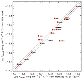
Figure 18: Comparison of 7510 Å fluxes from our work and from Herczeg & Hillenbrand (2014). The open circle also locates our 7510 Å flux for V409 Tau with respect to the SDSS photometry. The dash line shows the 1:1 line while dotted lines mark a $\pm$0.04 dex difference.

We use 3 spectrophotometric standards each night to flux calibrate the spectra of our scientific targets. First, we obtain the BT-settl model atmosphere (Allard et al., 2011) corresponding to each telluric standard spectral type in the night of January 23, 2008, and the white dwarf model atmosphere (Koester, 2010) for the white dwarf telluric standards in the night of May 23, 2008. Next, we fit its broad-band photometry using the aforementioned model with two free parameters, extinction and stellar angular radius as in Fang et al. (2009, 2013a). Then, we shift and rotationally broaden the best-fit model atmosphere and degrade it to the Keck spectral resolution. In each order, the ratio between the observed and model spectrum is fitted with a 4-order polynomial function, from which we obtain the conversion from counts to absolute flux. The spectrophotometric standard that is observed closest in time to each of our target is chosen its flux calibration. As our slit width is narrow (0$\farcs$861), we also correct for the missing flux due to the difference in point source functions between the target and the spectrophotometric standard. Atmospheric absorption due to the different airmass between the spectrophotometric standards and the scientific objects is also corrected using optical extinction coefficients proper for Mauna Kea . The flux calibration did not account for atmospheric dispersion in the observations of DK Tau where the slit position angle was offset from the parallactic angle. For SCrA A+B, the MAKEE pipeline cannot resolve the SCrA A and B components, and thus the flux calibration over-correct the flux for the slit loss by $\sim$20%.

We use two methods to estimate the uncertainty on the flux-calibration. The first one is to flux calibrate one spectrophotometric standard using another close-in-time spectrophotometric, and compare the calibrated flux with the expected one. We found differences of $\sim$14% for the night on January 23, 2008 and only $\sim$3% for the night on May 23, 2008. To evaluate the uncertainty on line ratios close to the forbidden lines analyzed here, we also calculate the $F_{\rm cont,4068}/F_{\rm cont,6300}$ and the $F_{\rm cont,5577}/F_{\rm cont,6300}$, basically continuum fluxes near the [S II] $\lambda$4068  [O I] $\lambda$5577, and [O I] $\lambda$6300 transitions, from the flux-calibrated spectra of one spectrophotometric standard using another one close in time. When comparing them with the expected values, we find differences of $\sim$5% and 3% on January 23, 2008 and $\sim$5% and 1% on May 23, 2008 for the $F_{\rm cont,4068}/F_{\rm cont,6300}$ and $F_{\rm cont,5577}/F_{\rm cont,6300}$ ratios, respectively.

The data acquired on January 23, 2008 cover wavelengths near 7510 Å. Hence, we can further estimate the uncertainty on our flux calibration by comparing our calibrated 7510 Å fluxes with those reported in Herczeg & Hillenbrand (2014). Unfortunately, the 7510 Å wavelength is located in the gap between two HIRES orders. So, we did not measure the 7510 Å flux directly, but instead interpolate the flux using wavelengths near 7510 Å. Figure 18 shows our flux values compared to those from Herczeg & Hillenbrand (2014). The mean difference between the two works is about 0.07 dex. Four sources, DS Tau, HN TauA, GI Tau, and V409 Tau, show larger differences (0.10-0.37 dex), which may be due to their brightness variability (see Rodriguez et al. 2015 for V409 Tau and Guo et al. 2018 for GI Tau). V409 Tau, which sports the largest difference (0.37 dex), has been also observed with SDSS (Ahn et al., 2012) and is 11.934 mag in $SDSS-i$ band. We convert the $i$-band photometry to flux and correct for the extinction $A_{\rm V}$=1 from Herczeg & Hillenbrand (2014), which gives a flux of 5.76$\times$10^-14 erg s^-1 cm^-2 Å^-1 at 7625 Å (the center of $SDSS-i$ band). The difference between our 7510 Å flux and the SDSS 7625 Å flux is $\sim$0.09 dex, much lower than that with Herczeg & Hillenbrand (2014), which supports the hypothesis of variability driving a larger difference. If we exclude the four outliers in Figure 18, the mean difference between our 7510 Å fluxes and those from Herczeg & Hillenbrand (2014) is reduced to $\sim$0.03 dex. In summary, two different methods suggest that the uncertainty on our absolute flux calibration is likely better than 10%.

Appendix C Comments on sources without [O I] $\lambda$6300 detection

Our sample includes three sources (Sz 68A, DoAr 21, and DoAr 24E) with no [O I] $\lambda$6300 detection. Neither DoAr 21 nor DoAr 24E show emission lines in our spectra that can be used to derive accretion luminosities and thus are inferred to have weak or absent disk accretion. In the following, we provide additional information on these sources.

Sz 68A is a a triple system with a close binary (separation 0$\farcs$126) and a third faint companion (M6) with a separation of 2$\farcs$808 (Correia et al., 2006). Our spectroscopic observation targeted the close binary. We detect the Ca  II lines at 3934 and 3968 Å but only weak H$\alpha$ emission ($EW\sim-$2.8Å). This star has been classified as a weak-line T Tauri star, a young non-accreting star, by Cieza et al. (2007) and Alcalá et al. (2017). The [O I] $\lambda$6300 emission is not detected in our HIRES spectra and it is also absent in the X-Shooter spectra by Nisini et al. (2018). Ansdell et al. (2016) reported cold CO gas emission around the binary and no gas or dust cavity at a resolution of 50$\times$40 au. The SED of Sz 68A is compatible with that of a full disk.

DoAr 21 is a close binary with a separation of 1.2–1.8 au (Loinard et al., 2008). The HIRES spectrum of DoAr 21, which covers from 4420 to 6310 Å, does not show any accretion-related emission lines. Salyk et al. (2013) detected Pf$\beta$ emission from DoAr 21 and estimated a mass accretion rate of 1.7$\times 10^{-8}$ M_⊙ yr^-1. DoAr 21 is detected at far-infrared wavelengths (Rebollido et al., 2015) and has reduced mid-infrared emission as TDs (see Fig. 14 from our paper). However, based on high spatial resolution mid-infrared imagery, Jensen et al. (2009) find very weak, almost absent, excess emission from this source at 9–18 µm and argue that low resolution data could be contaminated by an extended infrared source. Thus, they suggested that either the disk is in the final stage of clearing, or there is no disk around DoAr 21. The recent ALMA imaging of DoAr 21 at 870  $\mu$m shows no detection at a spatial resolution 0$\farcs$2 and a sensitivity 0.02 mJy (Cox et al., 2017). Therefore, even if there is a disk around DoAr 21, its disk mass should be very low.

DoAr 24E has a faint companion at a separation of 2$\farcs$03 (Ratzka et al., 2005). Our HIRES spectrum covering from 4420 to 6310 Å does not show any accretion-related emission lines. Natta et al. (2006) detected Pa$\beta$ emission from its near-infrared spectrum and estimated a mass accretion rate of 6.2$\times 10^{-9}$ M_⊙ yr^-1. The source SED is compatible with that of full disks. The continuum emission from the disk has been detected at far-infrared, sub-millimeter, and millimeter wavelengths (Rebollido et al., 2015; Mohanty et al., 2013). No [O I] and o-H₂O emission is detected around 63  $\mu$m (Riviere-Marichalar et al., 2016).

Appendix D Corrected line profiles and kinematic decomposition

The rationale for decomposing corrected line profiles with Gaussians is discussed in Sect.  3.2 while the best fit parameters are summarized in Table 2. Fig. 20 provides the best fit Gaussian profiles color coded by kinematic component and superimposed on the corrected [S II] $\lambda$4068, [O I] $\lambda$5577, and [O I] $\lambda$6300 profiles for all the sources in our sample.

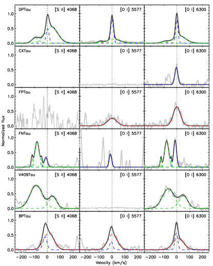
Figure 19: [S II] $\lambda$4068  [O I] $\lambda$6300  and [O I] $\lambda$5577 line profiles for our sample. In each panel, the green dashed line is for the HVC, the red dashed line for the LVC-BC, the blue dashed line for the LVC-NC, and the dark solid line is the sum of all components. For EX Lup, Fe lines contaminating the profiles of the forbidden lines are marked with vertical dashed light blue lines.

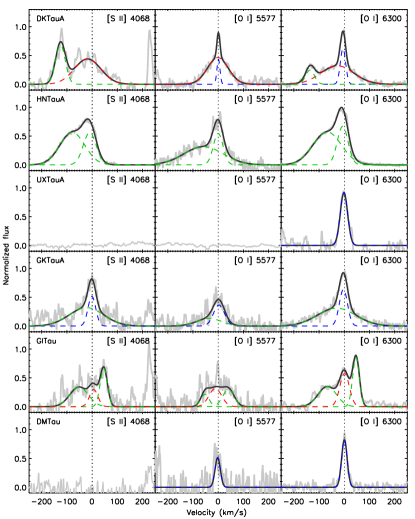
Figure 20: continued.

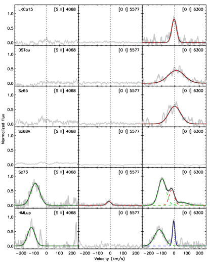
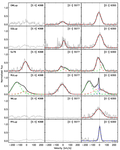
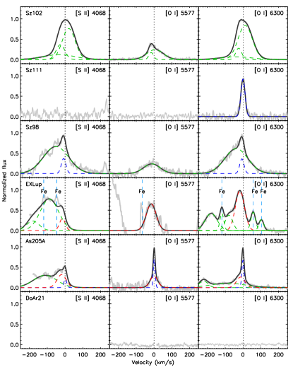
Figure 20: continued.

Figure 20: continued.

Figure 20: continued.

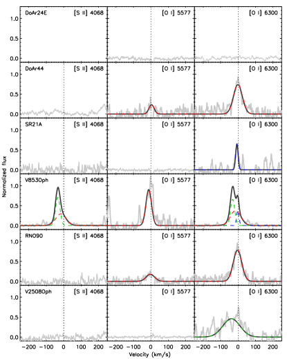
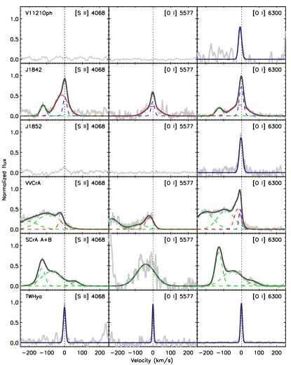
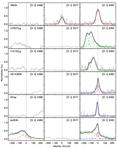
Figure 20: continued.

Figure 20: continued.

Figure 20: continued.

Appendix E Line decontamination

Seven sources present [S II] $\lambda$4068 line profiles that are highly contaminated by Fe I emission at 4063.6 and 4071.7 Å. In addition, the [O I] $\lambda$5577 line from RU Lup is also contaminated by Fe I emission at 5572.8 Å. Fig. 21 shows the contaminated line profiles. We fit the wings of the Fe I emission with linear functions and tentatively decontaminate the profiles by subtracting the fitted function from the observed spectra. The corrected [S II] $\lambda$4068 and [O I] $\lambda$5577 line profiles are also shown in Fig. 21. Due to the strong contamination from the Fe I line at 4063.6 Å, any [S II] $\lambda$4068  flux more blueshifted than $\sim$200  km s^-1 cannot be recovered. A comparison of [S II] $\lambda$4068 and [O I] $\lambda$6300 profiles suggest that we achieve a good correction for less blueshifted emission (see Fig. 5 in the main text).

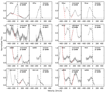
Figure 21: Profiles that are contaminated by Fe I lines (left panels). The right panels show our corrected profiles.

Appendix F A comparison of the individual components in [S II] $\lambda$4068 and [O I] $\lambda$6300

As discussed in the main text (Sect.  4.1), individual kinematic components present similar [S II] $\lambda$4068, [O I] $\lambda$5577, and [O I] $\lambda$6300 profiles indicating they trace the same physical region. Here, we provide further evidence to this finding by showing a comparison of centroids and FWHMs of individual [S II] $\lambda$4068 and [O I] $\lambda$5577 components vs the [O I] $\lambda$6300 components (see Figure 22). Note the similarity in centroids and FWHMs for individual kinematic components.

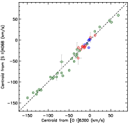
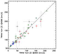
Figure 22: Centroids (left) and FWHMs (right) of individual [S II] $\lambda$4068 and [O I] $\lambda$6300 components (HVC in green, LVC-BC in red, and LVC-NC in blue). A dashed line shows the 1:1 relation.

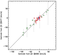
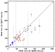
Figure 23: Same as Fig. 22 but for the [O I] $\lambda$5577 and [O I] $\lambda$6300 lines.

Appendix G Updated relation between line and accretion luminosity

In view of the Gaia DR2 release (Bailer-Jones et al., 2018), we revisit the relations between the luminosity of permitted lines ($L_{\rm line}$) and the accretion luminosity ($L_{\rm acc}$). We collect $L_{\rm line}$ and $L_{\rm acc}$ from Alcalá et al. (2017) and scale them to the new Gaia DR2 distance of each source. We carry out a linear regression to fit: Log $L_{\rm acc}$=a$\times$Log $L_{\rm line}$+b. We have excluded weak (or dubious) accretors and sub-luminous objects from the fit. The best fit $a$ and $b$ coefficients and their uncertainties are listed in Table 7. Within 1$\sigma$, most of them are the same as those reported in Alcalá et al. (2017).

Table 7: Revised Log $L_{\rm acc}$–Log $L_{\rm line}$ linear fit

Lines	$\lambda$ (Å)	a($\pm$err)	b($\pm$err)
H${\alpha}$	6562.80	1.15($\pm$ 0.05)	1.81($\pm$ 0.20)
H${\beta}$	4861.33	1.15($\pm$ 0.03)	2.64($\pm$ 0.16)
H${\gamma}$	4340.46	1.12($\pm$ 0.03)	2.75($\pm$ 0.17)
H${\delta}$	4101.73	1.09($\pm$ 0.04)	2.74($\pm$ 0.19)
H${\zeta}$	3889.05	1.06($\pm$ 0.03)	2.76($\pm$ 0.18)
Pa$\beta$	12818.07	1.08($\pm$ 0.07)	2.81($\pm$ 0.36)
Pa$\gamma$	10938.09	1.21($\pm$ 0.06)	3.43($\pm$ 0.29)
Pa$\delta$	10049.37	1.27($\pm$ 0.09)	3.93($\pm$ 0.44)
Br$\gamma$	21661.2	1.20($\pm$ 0.11)	4.07($\pm$ 0.57)
He I	4026.19	1.05($\pm$ 0.04)	3.67($\pm$ 0.22)
He I	4471.48	1.05($\pm$ 0.04)	3.48($\pm$ 0.23)
He I	4713.15	0.86($\pm$ 0.08)	3.02($\pm$ 0.50)
He I	5015.68	1.01($\pm$ 0.04)	3.61($\pm$ 0.24)
He I	5875.62	1.17($\pm$ 0.04)	3.78($\pm$ 0.22)
He I	6678.15	1.24($\pm$ 0.06)	4.71($\pm$ 0.34)
He I	7065.19	1.20($\pm$ 0.05)	4.57($\pm$ 0.29)
He II	4685.80	1.05($\pm$ 0.05)	3.90($\pm$ 0.33)
Ca II (K)	3933.66	1.05($\pm$ 0.04)	2.60($\pm$ 0.18)
Ca II (H)	3968.47	1.09($\pm$ 0.03)	2.78($\pm$ 0.16)

References

- Agra-Amboage et al. (2011) Agra-Amboage, V., Dougados, C., Cabrit, S., & Reunanen, J. 2011, A&A, 532, A59
- Ahn et al. (2012) Ahn, C. P., Alexandroff, R., Allende Prieto, C., et al. 2012, ApJS, 203, 21
- Alcalá et al. (2014) Alcalá, J. M., Natta, A., Manara, C. F., et al. 2014, A&A, 561, A2
- Alcalá et al. (2017) Alcalá, J. M., Manara, C. F., Natta, A., et al. 2017, A&A, 600, A20
- Alexander (2008) Alexander, R. D. 2008, MNRAS, 391, L64
- Allard et al. (2011) Allard, F., Homeier, D., & Freytag, B. 2011, in Astronomical Society of the Pacific Conference Series, Vol. 448, 16th Cambridge Workshop on Cool Stars, Stellar Systems, and the Sun, ed. C. Johns-Krull, M. K. Browning, & A. A. West, 91
- Andrews et al. (2010) Andrews, S. M., Wilner, D. J., Hughes, A. M., Qi, C., & Dullemond, C. P. 2010, ApJ, 723, 1241
- Ansdell et al. (2016) Ansdell, M., Williams, J. P., van der Marel, N., et al. 2016, ApJ, 828, 46
- Armitage et al. (2013) Armitage, P. J., Simon, J. B., & Martin, R. G. 2013, ApJ, 778, L14
- Asplund et al. (2005) Asplund, M., Grevesse, N., & Sauval, A. J. 2005, in Astronomical Society of the Pacific Conference Series, Vol. 336, Cosmic Abundances as Records of Stellar Evolution and Nucleosynthesis, ed. T. G. Barnes, III & F. N. Bash, 25
- Audard et al. (2014) Audard, M., Ábrahám, P., Dunham, M. M., et al. 2014, Protostars and Planets VI, 387
- Bacciotti et al. (2000) Bacciotti, F., Mundt, R., Ray, T. P., et al. 2000, ApJ, 537, L49
- Bacciotti et al. (2002) Bacciotti, F., Ray, T. P., Mundt, R., Eislöffel, J., & Solf, J. 2002, ApJ, 576, 222
- Bai (2014) Bai, X.-N. 2014, ApJ, 791, 137
- Bai (2017) —. 2017, ApJ, 845, 75
- Bai & Stone (2013) Bai, X.-N., & Stone, J. M. 2013, ApJ, 769, 76
- Bai & Stone (2017) —. 2017, ApJ, 836, 46
- Bailer-Jones et al. (2018) Bailer-Jones, C. A. L., Rybizki, J., Fouesneau, M., Mantelet, G., & Andrae, R. 2018, ArXiv e-prints, arXiv:1804.10121 [astro-ph.SR]
- Banzatti et al. (2018) Banzatti, A., Pascucci, I., Edwards, S., Fang, M., Gorti, U., & Flock, M. 2018, submitted
- Beck et al. (2010) Beck, T. L., Bary, J. S., & McGregor, P. J. 2010, ApJ, 722, 1360
- Bertaux et al. (2014) Bertaux, J. L., Lallement, R., Ferron, S., Boonne, C., & Bodichon, R. 2014, A&A, 564, A46
- Béthune et al. (2017) Béthune, W., Lesur, G., & Ferreira, J. 2017, A&A, 600, A75
- Blandford & Payne (1982) Blandford, R. D., & Payne, D. G. 1982, MNRAS, 199, 883
- Bustamante et al. (2015) Bustamante, I., Merín, B., Ribas, Á., et al. 2015, A&A, 578, A23
- Cabrit (2009) Cabrit, S. 2009, Astrophysics and Space Science Proceedings, 13, 247
- Cieza et al. (2007) Cieza, L., Padgett, D. L., Stapelfeldt, K. R., et al. 2007, ApJ, 667, 308
- Cohen & Kuhi (1979) Cohen, M., & Kuhi, L. V. 1979, The Astrophysical Journal Supplement Series, 41, 743
- Correia et al. (2006) Correia, S., Zinnecker, H., Ratzka, T., & Sterzik, M. F. 2006, A&A, 459, 909
- Cox et al. (2017) Cox, E. G., Harris, R. J., Looney, L. W., et al. 2017, ApJ, 851, 83
- Dere et al. (1997) Dere, K. P., Landi, E., Mason, H. E., Monsignori Fossi, B. C., & Young, P. R. 1997, A&AS, 125, 149
- Donaldson et al. (2016) Donaldson, J. K., Weinberger, A. J., Gagné, J., et al. 2016, ApJ, 833, 95
- Dougados et al. (2010) Dougados, C., Bacciotti, F., Cabrit, S., & Nisini, B. 2010, in Lecture Notes in Physics, Berlin Springer Verlag, Vol. 793, Lecture Notes in Physics, Berlin Springer Verlag, ed. P. J. V. Garcia & J. M. Ferreira, 213
- Dunham et al. (2015) Dunham, M. M., Allen, L. E., Evans, II, N. J., et al. 2015, ApJS, 220, 11
- Edwards et al. (1987) Edwards, S., Cabrit, S., Strom, S. E., et al. 1987, ApJ, 321, 473
- Ercolano & Owen (2016) Ercolano, B., & Owen, J. E. 2016, MNRAS, 460, 3472
- Ercolano & Pascucci (2017) Ercolano, B., & Pascucci, I. 2017, Royal Society Open Science, 4, 170114
- Espaillat et al. (2014) Espaillat, C., Muzerolle, J., Najita, J., et al. 2014, Protostars and Planets VI, 497
- Evans et al. (2014) Evans, II, N. J., Allen, L. E., Blake, G. A., et al. 2014, VizieR Online Data Catalog, 2332
- Fang et al. (2013a) Fang, M., Kim, J. S., van Boekel, R., et al. 2013a, ApJS, 207, 5
- Fang et al. (2013b) Fang, M., van Boekel, R., Bouwman, J., et al. 2013b, A&A, 549, A15
- Fang et al. (2009) Fang, M., van Boekel, R., Wang, W., et al. 2009, A&A, 504, 461
- Fang et al. (2017) Fang, Q., Herczeg, G. J., & Rizzuto, A. 2017, ApJ, 842, 123
- Feiden (2016) Feiden, G. A. 2016, A&A, 593, A99
- Feigelson & Nelson (1985) Feigelson, E. D., & Nelson, P. I. 1985, ApJ, 293, 192
- Ferreira et al. (2006) Ferreira, J., Dougados, C., & Cabrit, S. 2006, A&A, 453, 785
- Frank et al. (2014) Frank, A., Ray, T. P., Cabrit, S., et al. 2014, Protostars and Planets VI, 451
- Frasca et al. (2017) Frasca, A., Biazzo, K., Alcalà, J. M., et al. 2017, ArXiv e-prints, arXiv:1703.01251 [astro-ph.SR]
- Fromang et al. (2013) Fromang, S., Latter, H., Lesur, G., & Ogilvie, G. I. 2013, A&A, 552, A71
- Gammie (1996) Gammie, C. F. 1996, ApJ, 457, 355
- Giannini et al. (2015) Giannini, T., Antoniucci, S., Nisini, B., Bacciotti, F., & Podio, L. 2015, ApJ, 814, 52
- Giannini et al. (2013) Giannini, T., Nisini, B., Antoniucci, S., et al. 2013, ApJ, 778, 71
- Gorti et al. (2011) Gorti, U., Hollenbach, D., Najita, J., & Pascucci, I. 2011, ApJ, 735, 90
- Gorti et al. (2016) Gorti, U., Liseau, R., Sándor, Z., & Clarke, C. 2016, Space Sci. Rev., 205, 125
- Green et al. (2006) Green, J. D., Hartmann, L., Calvet, N., et al. 2006, ApJ, 648, 1099
- Gressel et al. (2015) Gressel, O., Turner, N. J., Nelson, R. P., & McNally, C. P. 2015, ApJ, 801, 84
- Guilloteau et al. (2011) Guilloteau, S., Dutrey, A., Piétu, V., & Boehler, Y. 2011, A&A, 529, A105
- Gullbring et al. (1998) Gullbring, E., Hartmann, L., Briceno, C., & Calvet, N. 1998, ApJ, 492, 323
- Guo et al. (2018) Guo, Z., Herczeg, G. J., Jose, J., et al. 2018, ApJ, 852, 56
- Hales et al. (2018) Hales, A. S., Peréz, S., Saito, M., et al. 2018, ArXiv e-prints, arXiv:1804.10340 [astro-ph.SR]
- Harich et al. (2000) Harich, S. A., Hwang, D. W. H., Yang, X., et al. 2000, J. Chem. Phys., 113, 10073
- Hartigan et al. (1995) Hartigan, P., Edwards, S., & Ghandour, L. 1995, ApJ, 452, 736
- Hartigan et al. (1989) Hartigan, P., Hartmann, L., Kenyon, S., Hewett, R., & Stauffer, J. 1989, ApJS, 70, 899
- Hartigan & Morse (2007) Hartigan, P., & Morse, J. 2007, ApJ, 660, 426
- Hartigan et al. (1994) Hartigan, P., Morse, J. A., & Raymond, J. 1994, ApJ, 436, 125
- Hartigan et al. (1987) Hartigan, P., Raymond, J., & Hartmann, L. 1987, ApJ, 316, 323
- Hartigan & Wright (2015) Hartigan, P., & Wright, A. 2015, ApJ, 811, 12
- Herbig (1977) Herbig, G. H. 1977, ApJ, 217, 693
- Herbig & Bell (1988) Herbig, G. H., & Bell, K. R. 1988, Third Catalog of Emission-Line Stars of the Orion Population : 3 : 1988
- Herbig et al. (2003) Herbig, G. H., Petrov, P. P., & Duemmler, R. 2003, ApJ, 595, 384
- Herczeg & Hillenbrand (2008) Herczeg, G. J., & Hillenbrand, L. A. 2008, ApJ, 681, 594
- Herczeg & Hillenbrand (2014) —. 2014, ApJ, 786, 97
- Hillenbrand et al. (2008) Hillenbrand, L. A., Carpenter, J. M., Kim, J. S., et al. 2008, ApJ, 677, 630
- Hirth et al. (1997) Hirth, G. A., Mundt, R., & Solf, J. 1997, A&AS, 126, 437
- Hollenbach & Gorti (2009) Hollenbach, D., & Gorti, U. 2009, ApJ, 703, 1203
- Hollenbach & McKee (1979) Hollenbach, D., & McKee, C. F. 1979, ApJS, 41, 555
- Hollenbach & McKee (1989) —. 1989, ApJ, 342, 306
- Howard et al. (2013) Howard, C. D., Sandell, G., Vacca, W. D., et al. 2013, ApJ, 776, 21
- Hughes et al. (2010) Hughes, A. M., Andrews, S. M., Wilner, D. J., et al. 2010, AJ, 140, 887
- Husser et al. (2013) Husser, T.-O., Wende-von Berg, S., Dreizler, S., et al. 2013, A&A, 553, A6
- Jenkins (2009) Jenkins, E. B. 2009, ApJ, 700, 1299
- Jensen et al. (2009) Jensen, E. L. N., Cohen, D. H., & Gagné, M. 2009, ApJ, 703, 252
- Johns-Krull et al. (2000) Johns-Krull, C. M., Valenti, J. A., & Linsky, J. L. 2000, ApJ, 539, 815
- Kennedy & Kenyon (2009) Kennedy, G. M., & Kenyon, S. J. 2009, ApJ, 695, 1210
- Kenyon et al. (1998) Kenyon, S. J., Brown, D. I., Tout, C. A., & Berlind, P. 1998, AJ, 115, 2491
- Koester (2010) Koester, D. 2010, Mem. Soc. Astron. Italiana, 81, 921
- Lavalley-Fouquet et al. (2000) Lavalley-Fouquet, C., Cabrit, S., & Dougados, C. 2000, A&A, 356, L41
- Lazareff et al. (2017) Lazareff, B., Berger, J. P., Kluska, J., et al. 2017, A&A, 599, A85
- Lindegren et al. (2018) Lindegren, L., Hernandez, J., Bombrun, A., et al. 2018, ArXiv e-prints, arXiv:1804.09366 [astro-ph.IM]
- Loinard et al. (2008) Loinard, L., Torres, R. M., Mioduszewski, A. J., & Rodríguez, L. F. 2008, ApJ, 675, L29
- Louvet et al. (2016) Louvet, F., Dougados, C., Cabrit, S., et al. 2016, A&A, 596, A88
- Luhman et al. (2010) Luhman, K. L., Allen, P. R., Espaillat, C., Hartmann, L., & Calvet, N. 2010, ApJS, 186, 111
- Luhman & Mamajek (2012) Luhman, K. L., & Mamajek, E. E. 2012, ApJ, 758, 31
- Luhman et al. (2009) Luhman, K. L., Mamajek, E. E., Allen, P. R., & Cruz, K. L. 2009, ApJ, 703, 399
- Luhman & Rieke (1999) Luhman, K. L., & Rieke, G. H. 1999, ApJ, 525, 440
- MacGregor et al. (2017) MacGregor, M. A., Wilner, D. J., Czekala, I., et al. 2017, ApJ, 835, 17
- Manara et al. (2017) Manara, C. F., Frasca, A., Alcalá, J. M., et al. 2017, A&A, 605, A86
- Manara et al. (2015) Manara, C. F., Testi, L., Natta, A., & Alcalá, J. M. 2015, A&A, 579, A66
- Manara et al. (2014) Manara, C. F., Testi, L., Natta, A., et al. 2014, A&A, 568, A18
- Matt & Pudritz (2005) Matt, S., & Pudritz, R. E. 2005, ApJ, 632, L135
- Maurri et al. (2014) Maurri, L., Bacciotti, F., Podio, L., et al. 2014, A&A, 565, A110
- McGinnis et al. (2018) McGinnis, P., Dougados, C., Alencar, S. H. P., Cabrit, S., & Bouvier, J. 2018, ArXiv e-prints, arXiv:1803.10287 [astro-ph.SR]
- Mohanty et al. (2013) Mohanty, S., Greaves, J., Mortlock, D., et al. 2013, ApJ, 773, 168
- Najita et al. (2015) Najita, J. R., Andrews, S. M., & Muzerolle, J. 2015, MNRAS, 450, 3559
- Natta et al. (2014) Natta, A., Testi, L., Alcalá, J. M., et al. 2014, A&A, 569, A5
- Natta et al. (2006) Natta, A., Testi, L., & Randich, S. 2006, A&A, 452, 245
- Nisini et al. (2018) Nisini, B., Antoniucci, S., Alcalá, J. M., et al. 2018, A&A, 609, A87
- Pascucci et al. (2015) Pascucci, I., Edwards, S., Heyer, M., et al. 2015, ApJ, 814, 14
- Pelletier & Pudritz (1992) Pelletier, G., & Pudritz, R. E. 1992, ApJ, 394, 117
- Piétu et al. (2014) Piétu, V., Guilloteau, S., Di Folco, E., Dutrey, A., & Boehler, Y. 2014, A&A, 564, A95
- Pontoppidan et al. (2011) Pontoppidan, K. M., Blake, G. A., & Smette, A. 2011, ApJ, 733, 84
- Pudritz et al. (2007) Pudritz, R. E., Ouyed, R., Fendt, C., & Brandenburg, A. 2007, Protostars and Planets V, 277
- Pudritz et al. (2006) Pudritz, R. E., Rogers, C. S., & Ouyed, R. 2006, MNRAS, 365, 1131
- Pyo et al. (2002) Pyo, T.-S., Hayashi, M., Kobayashi, N., et al. 2002, ApJ, 570, 724
- Pyo et al. (2003) Pyo, T.-S., Kobayashi, N., Hayashi, M., et al. 2003, ApJ, 590, 340
- Ratzka et al. (2005) Ratzka, T., Köhler, R., & Leinert, C. 2005, A&A, 437, 611
- Rebollido et al. (2015) Rebollido, I., Merín, B., Ribas, Á., et al. 2015, A&A, 581, A30
- Rebull et al. (2010) Rebull, L. M., Padgett, D. L., McCabe, C.-E., et al. 2010, ApJS, 186, 259
- Rice et al. (2006) Rice, E. L., Prato, L., & McLean, I. S. 2006, ApJ, 647, 432
- Rigliaco et al. (2012) Rigliaco, E., Natta, A., Testi, L., et al. 2012, A&A, 548, A56
- Rigliaco et al. (2013) Rigliaco, E., Pascucci, I., Gorti, U., Edwards, S., & Hollenbach, D. 2013, ApJ, 772, 60
- Riviere-Marichalar et al. (2016) Riviere-Marichalar, P., Merín, B., Kamp, I., Eiroa, C., & Montesinos, B. 2016, A&A, 594, A59
- Riviere-Marichalar et al. (2013) Riviere-Marichalar, P., Pinte, C., Barrado, D., et al. 2013, A&A, 555, A67
- Rodriguez et al. (2015) Rodriguez, J. E., Pepper, J., Stassun, K. G., et al. 2015, AJ, 150, 32
- Romanova et al. (2009) Romanova, M. M., Ustyugova, G. V., Koldoba, A. V., & Lovelace, R. V. E. 2009, MNRAS, 399, 1802
- Safier (1993) Safier, P. N. 1993, ApJ, 408, 115
- Salyk et al. (2013) Salyk, C., Herczeg, G. J., Brown, J. M., et al. 2013, ApJ, 769, 21
- Sartori et al. (2003) Sartori, M. J., Lépine, J. R. D., & Dias, W. S. 2003, A&A, 404, 913
- Savage & Sembach (1996) Savage, B. D., & Sembach, K. R. 1996, ARA&A, 34, 279
- Scicluna et al. (2016) Scicluna, P., Wolf, S., Ratzka, T., et al. 2016, MNRAS, 458, 2476
- Shang et al. (2007) Shang, H., Li, Z.-Y., & Hirano, N. 2007, Protostars and Planets V, 261
- Shu (1977) Shu, F. H. 1977, ApJ, 214, 488
- Shull & McKee (1979) Shull, J. M., & McKee, C. F. 1979, ApJ, 227, 131
- Sicilia-Aguilar et al. (2011) Sicilia-Aguilar, A., Henning, T., Kainulainen, J., & Roccatagliata, V. 2011, ApJ, 736, 137
- Sicilia-Aguilar et al. (2013) Sicilia-Aguilar, A., Henning, T., Linz, H., et al. 2013, A&A, 551, A34
- Simon et al. (2017) Simon, M., Guilloteau, S., Di Folco, E., et al. 2017, ApJ, 844, 158
- Simon et al. (2016) Simon, M. N., Pascucci, I., Edwards, S., et al. 2016, ApJ, 831, 169
- Skrutskie et al. (2006) Skrutskie, M. F., Cutri, R. M., Stiening, R., et al. 2006, AJ, 131, 1163
- Suzuki & Inutsuka (2009) Suzuki, T. K., & Inutsuka, S.-i. 2009, ApJ, 691, L49
- Takami et al. (2004) Takami, M., Chrysostomou, A., Ray, T. P., et al. 2004, A&A, 416, 213
- Tazzari et al. (2017) Tazzari, M., Testi, L., Natta, A., et al. 2017, A&A, 606, A88
- Tripathi et al. (2017) Tripathi, A., Andrews, S. M., Birnstiel, T., & Wilner, D. J. 2017, ApJ, 845, 44
- van der Marel et al. (2016) van der Marel, N., Verhaar, B. W., van Terwisga, S., et al. 2016, A&A, 592, A126
- van der Marel et al. (2018) van der Marel, N., Williams, J. P., Ansdell, M., et al. 2018, ArXiv e-prints, arXiv:1801.06154 [astro-ph.EP]
- Varga et al. (2018) Varga, J., Ábrahám, P., Chen, L., et al. 2018, ArXiv e-prints, arXiv:1805.02939 [astro-ph.SR]
- Vogt et al. (1994) Vogt, S. S., Allen, S. L., Bigelow, B. C., et al. 1994, in Proc. SPIE, Vol. 2198, Instrumentation in Astronomy VIII, ed. D. L. Crawford & E. R. Craine, 362
- Wahhaj et al. (2010) Wahhaj, Z., Cieza, L., Koerner, D. W., et al. 2010, ApJ, 724, 835
- Woitas et al. (2002) Woitas, J., Ray, T. P., Bacciotti, F., Davis, C. J., & Eislöffel, J. 2002, ApJ, 580, 336
- Wright et al. (2010) Wright, E. L., Eisenhardt, P. R. M., Mainzer, A. K., et al. 2010, AJ, 140, 1868
- Zanni & Ferreira (2009) Zanni, C., & Ferreira, J. 2009, A&A, 508, 1117