Hadronic Molecular States Composed of Spin-$3\over 2$ Singly Charmed Baryons

Abstract

We investigate the possible deuteron-like molecules composed of a pair of charmed spin-$\frac{3}{2}$ baryons, or one charmed baryon and one charmed antibaryon within the one-boson-exchange (OBE) model. For the spin singlet and triplet systems, we consider the couple channel effect between systems with different orbital angular momentum. Most of the systems have binding solutions. The couple channel effect plays a significant role in the formation of some loosely bound states. The possible molecular states of $\Omega_{c}^{*}\Omega_{c}^{*}$ might be stable once produced.

1 INTRODUCTION

Since the charmonium-like state $X(3872)$ was reported by the Belle Collaboration in 2003 Choi:2003ue , exotic states attracted great interest around the world. Many experiment collaborations such as BaBar, BESIII, Belle, LHCb, CDF, D0, reported discoveries of new charmonium-like and bottomonium-like states such as $Y(4260)$ Aubert:2005rm , $Z_{c}(3900)$ Liu:2013dau ; Ablikim:2013mio , $Z_{b}(10610)$ and $Z_{b}(10650)$ Belle:2011aa . In 2015, LHCb reported two hidden-charm pentaquark states $P_{c}(4380)$ and $P_{c}(4450)$ Aaij:2015tga . One can find the experimental and theoretical progress about these exotic states in the recent reviews Chen:2016qju ; Esposito:2016noz ; Chen:2016spr ; Lebed:2016hpi ; Guo:2017jvc ; Olsen:2017bmm

It is difficult to interpret some of these states with the conventional quark model. They may well be multi-quark states rather than traditional $q\bar{q}$ and $qqq$ hadrons. Some of them are well studied as dynamically generated bound states or resonances Kaiser:1995cy ; Oller:2000fj ; Khemchandani:2011et ; Lu:2014ina ; Montana:2017kjw ; Liang:2017ejq . For the exotic states near the threshold of two heavy hadrons, it is natural to consider them as candidates of molecular states. A hadronic molecular state is a loosely bound state composed of two color-singlet hadrons. The interaction is the residual force of the color interaction, which is usually described as one-boson-exchange (OBE) potential. The OBE model is very successful to explain the deuteron, a well-established hadronic molecular state composed of a neutron and a proton. The meson exchange force together with the S-D mixing effect render the deuteron a loosely bound state. The binding energy is about 2.225 MeV and root-mean-square radius is about 2.0 fm.

Voloshin and Okun proposed the hadronic molecular composed of two charmed mesons about forty years ago Voloshin:1976ap . De Rujula et al. also used the molecular model to interpret the $\psi(4040)$ as a $D^{*}\bar{D}^{*}$ molecule DeRujula:1976zlg . Törnqvist used the one-pion-exchange (OPE) potential to calculate the possible molecular state composed of one charmed meson and one charmed antimesonTornqvist:1993ng ; Tornqvist:1993vu .

There are also many other analyses about hadronic molecular states, such as the combination of two mesonsWong:2003xk ; Liu:2009ei ; Close:2009ag ; Ding:2009vj ; Sun:2011uh ; Li:2012ss ; Zhao:2014gqa , or two baryonsLee:2011rka ; Meguro:2011nr ; Li:2012bt ; Meng:2017fwb ; Meng:2017udf ; Vijande:2016nzk ; Carames:2015sya . Similarly, the hidden-charm(bottom) pentaquark states can be explained as a molecular state formed by one heavy meson and one heavy baryonWu:2010jy ; Yang:2011wz ; Chen:2015loa ; Roca:2015dva ; Yamaguchi:2017zmn ; Shimizu:2017xrg ; Yamaguchi:2016ote . In addition, some near threshold states might be treated as a compact core plus a molecular component, like X(3872)Ferretti:2013faa ; Ferretti:2014xqa ; Ferretti:2018tco .

In the Ref. Li:2012bt , Li et al. calculated the possible molecular states composed of two spin-$\frac{1}{2}$ heavy baryons with the OPE and OBE potential, respectively. They analysed the $\Lambda_{c}\Lambda_{c}$ system and considered the couple-channel effect of $\Sigma_{c}$ and $\Sigma_{c}^{*}$. In this work, we extend the same formalism to investigate the possible hadronic molecular states composed of two spin-$\frac{3}{2}$ singly charmed baryons. We adopt the OBE potential and take the couple channel effect between systems with different orbital angular momentum into consideration.

This work is organized as follows. After the introduction, we present the formalism in Section 2, in which we introduce the Lagrangians, coupling constants and the effective interaction potentials. In Section 3 we show our numerical results of the two heavy baryon systems. Then we discuss our results and conclude in Section 4. We collect some useful formulae and functions in Appendixes A and B. We also calculate the systems composed of one heavy baryon and one heavy antibaryon. The numerical results are collected in Appendix C.

2 FORMALISM

2.1 The Lagrangian

The singly charmed baryon is composed of one charm quark and two light quarks, which is usually treated as a diquark. In the heavy quark limit, we can classify the singly charmed baryons with symmetry of the light diquark. The wave function of the diquark is as follows,

$$\Psi^{total}_{qq}=\Psi^{flavor}_{qq}\otimes\Psi^{spin}_{qq}\otimes\Psi^{color}_{qq}\otimes\Psi^{spatial}_{qq}.$$ (1)

The total wave function $\Psi^{total}_{qq}$ is antisymmetric for a fermion system as required by Pauli Principle. The color wave function $\Psi^{color}_{qq}$ must be in antisymmetric $\bar{3}_{c}$-representation, and the spatial wave function $\Psi^{spatial}_{qq}$ is symmetric for the ground state. As a result, the flavor wave function $\Psi^{flavor}_{qq}$ and the spin wave function $\Psi^{spin}_{qq}$ are correlated with each other. When $\Psi^{flavor}_{qq}$ is symmetric in the $6_{f}$-representation, $\Psi^{spin}_{qq}$ must be symmetric, which means the spin of the diquark is 1. On the other hand, $\Psi^{flavor}_{qq}$ can also be antisymmetric in the $\bar{3}_{f}$-representation, and $\Psi^{spin}_{qq}$ must be antisymmetric, i.e., the spin of diquark is 0. Taking the spin of heavy quark into account, it is convenient to describe the charmed baryon with its total spin and the flavor representation of diquark. For the $6_{f}$-representation one, the total spin can be $\frac{1}{2}$ and $\frac{3}{2}$. For the $\bar{3}_{f}$-representation one, the total spin is $\frac{1}{2}$.

We denote the charmed baryons as Yan:1992gz :

$$\begin{split}B_{6}&=\left[\begin{array}[]{ccc}\Sigma_{c}^{++}&\frac{1}{\sqrt{2}}\Sigma_{c}^{+}&\frac{1}{\sqrt{2}}\Xi_{c}^{{}^{\prime}+}\\ \frac{1}{\sqrt{2}}\Sigma_{c}^{+}&\Sigma_{c}^{0}&\frac{1}{\sqrt{2}}\Xi_{c}^{{}^{\prime}0}\\ \frac{1}{\sqrt{2}}\Xi_{c}^{{}^{\prime}+}&\frac{1}{\sqrt{2}}\Xi_{c}^{{}^{\prime}0}&\Omega_{c}^{0}\end{array}\right],B_{\bar{3}}=\left[\begin{array}[]{ccc}0&\Lambda_{c}^{+}&\Xi_{c}^{+}\\ -\Lambda_{c}^{+}&0&\Xi_{c}^{0}\\ -\Xi_{c}^{+}&-\Xi_{c}^{0}&0\end{array}\right],\\ B_{6}^{*}&=\left[\begin{array}[]{ccc}\Sigma_{c}^{*++}&\frac{1}{\sqrt{2}}\Sigma_{c}^{*+}&\frac{1}{\sqrt{2}}\Xi_{c}^{*+}\\ \frac{1}{\sqrt{2}}\Sigma_{c}^{*+}&\Sigma_{c}^{*0}&\frac{1}{\sqrt{2}}\Xi_{c}^{*0}\\ \frac{1}{\sqrt{2}}\Xi_{c}^{*+}&\frac{1}{\sqrt{2}}\Xi_{c}^{*0}&\Omega_{c}^{*0}\end{array}\right].\end{split}$$ (2)

We use the superscript “ * ” to label spin-$\frac{3}{2}$ baryons. The matrices of exchanged pseudoscalar and vector bosons are as follows,

$$\mathcal{M} = \left[\begin{array}[]{ccc}\frac{\pi^{0}}{\sqrt{2}}+\frac{\eta}{\sqrt{6}}&\pi^{+}&K^{+}\\ \pi^{-}&-\frac{\pi^{0}}{\sqrt{2}}+\frac{\eta}{\sqrt{6}}&K^{0}\\ K^{-}&\bar{K}^{0}&-\frac{2}{\sqrt{6}}\eta\\ \end{array}\right],$$ (6)

$$\mathcal{V}^{\mu} = \left[\begin{array}[]{ccc}\frac{\rho^{0}}{\sqrt{2}}+\frac{\omega}{\sqrt{2}}&\rho^{+}&K^{*+}\\ \rho^{-}&-\frac{\rho^{0}}{\sqrt{2}}+\frac{\omega}{\sqrt{2}}&K^{*0}\\ K^{*-}&\bar{K}^{*0}&\phi\\ \end{array}\right]^{\mu}.$$ (10)

Under the SU(3)-flavor symmetry, the meson exchange Lagrangians are constructed as Liu:2011xc

$$\mathcal{L}=\mathcal{L}_{\sigma hh}+\mathcal{L}_{phh}+\mathcal{L}_{vhh},$$ (11)

for the scalar meson exchange

$$\mathcal{L}_{\sigma hh}=-g_{\sigma B_{6}^{*}B_{6}^{*}}Tr[\bar{B}_{6}^{*\mu}\sigma B_{6\mu}^{*}],$$ (12)

for the pseudoscalar meson exchange

$$\mathcal{L}_{phh}=-g_{pB_{6}^{*}B_{6}^{*}}Tr[\bar{B}_{6}^{*\mu}i\gamma_{5}\mathcal{M}B_{6\mu}^{*}],$$ (13)

and for the vector meson exchange

$$\begin{aligned} \mathcal{L}_{vhh}=&-g_{vB_{6}^{*}B_{6}^{*}}Tr[\bar{B}_{6}^{*\mu}\gamma_{\nu}\mathcal{V}^{\nu}B_{6\mu}^{*}]\\ &-i\frac{f_{vB_{6}^{*}B_{6}^{*}}}{2m_{6^{*}}}Tr[\bar{B}_{6\mu}^{*}(\partial^{\mu}\mathcal{V}^{\nu}-\partial^{\nu}V^{\mu})B_{6\nu}^{*}].\end{aligned}$$ (14)

The notations $g_{\sigma B_{6}^{*}B_{6}^{*}}$, $g_{pB_{6}^{*}B_{6}^{*}}$ and $g_{vB_{6}^{*}B_{6}^{*}}$, represent the coupling constants. $m_{6}^{*}$ is the mass of the spin $\frac{3}{2}$ heavy baryon in $6_{f}$-representation.

2.2 Coupling Constants

The coupling constants in Eqs. (12-14) can be determined with the help of the nucleon-nucleon-meson vertices. Comparing the relevant constants for heavy baryon with those for nucleon via the quark model, we can easily get the relationship between them. Some details can be found in Ref .Meng:2017fwb . Here we list the relationships we need in this work directly,

$$g_{\sigma B_{6}^{*}B_{6}^{*}}=\frac{2}{3}g_{\sigma NN},$$ (15)

$$g_{pB_{6}^{*}B_{6}^{*}}=\frac{6\sqrt{2}}{5}g_{\pi NN}\frac{m_{i}+m_{f}}{2m_{N}},$$ (16)

$$g_{vB_{6}^{*}B_{6}^{*}}=2\sqrt{2}g_{\rho NN},$$ (17)

$$g_{vB_{6}^{*}B_{6}^{*}}+f_{vB_{6}^{*}B_{6}^{*}}=\frac{6\sqrt{2}}{5}(g_{\rho NN}+f_{\rho NN})\frac{\sqrt{m_{i}m_{f}}}{m_{N}}$$ (18)

where the $g_{\sigma NN}$, $g_{\pi NN}$, $g_{\rho NN}$ and $f_{\rho NN}$, are the nucleon-nucleon-meson coupling constants. Their numerical values are taken from Refs. Machleidt:1987hj ; Riska:2000gd ; Machleidt:2000ge ; Cao:2010km . For the nucleon vertices, one can also choose coupling constants for other mesons such as $g_{\eta NN}$ and $g_{\omega NN}$. In this work, we select three representative numerical values as mentioned above, after consider their stability in various models. Their values are shown in Table 1. $m_{N}$ is the nucleon mass, $m_{i}$ and $m_{f}$ are the masses of initial state and final state baryon respectively. Thus, the numerical values of coupling constants for different baryon-baryon-meson vertices vary slightly. Their numerical values can be found in Table 2. The masses of baryons and exchanged mesons are collected in Table 1.

Table 1: The relevant hadron masses Tanabashi:2018oca and coupling constants for the nucleon Machleidt:1987hj ; Riska:2000gd ; Machleidt:2000ge ; Cao:2010km . For the multiple hadrons, their averaged masses are used.

Baryons	Mass(MeV)	Mesons	Mass(MeV)	Mesons	Mass(MeV)	Couplings	Value
$\Sigma_{c}^{*}$	2518.4	$\pi$	137.25	$\omega$	782.65	$g^{2}_{\sigma NN}/4\pi$	5.69
$\Xi_{c}^{*}$	2645.9	$\eta$	547.85	$\phi$	1019.46	$g^{2}_{\pi NN}/4\pi$	13.6
$\Omega_{c}^{*}$	2765.9	$\rho$	775.49	$\sigma$	600	$g^{2}_{\rho NN}/4\pi$	0.84
						$f_{\rho NN}/g_{\rho NN}$	6.1

Table 2: The coupling constants for the spin-$3\over 2$ charmed baryons.

Vertex	$g_{\sigma B_{6}^{*}B_{6}^{*}}$	$g_{pB_{6}^{*}B_{6}^{*}}$	$g_{vB_{6}^{*}B_{6}^{*}}$	$f_{vB_{6}^{*}B_{6}^{*}}$
$\Sigma_{c}^{*}\Sigma_{c}^{*}$	5.64	59.50	9.19	95.80
$\Xi_{c}^{*}\Xi_{c}^{*}$	5.64	62.51	9.19	101.12
$\Omega_{c}^{*}\Omega_{c}^{*}$	5.64	65.35	9.19	106.12

2.3 The Effective Interaction Potentials

With the Lagrangians in Eqs. (12-14), we can get the interaction potentials $\mathcal{V}(Q)$ in momentum space, which can be expanded in terms of the heavy baryon mass. We expand the potential up to $\mathcal{O}(\frac{1}{m_{Q}^{2}})$. Then we transform the potential to coordinate space through Fourier transformation.

$$\mathcal{V}(r)=\frac{1}{(2\pi)^{3}}\int d\textbf{Q}e^{i\textbf{Q}\cdot\textbf{r}}\mathcal{V}(\textbf{Q})\cdot\mathcal{F}^{2}(\textbf{Q})$$ (19)

A form factor $\mathcal{F}(Q)$ is introduced to suppress the contribution of high momentum transfer between baryons. Within the meson exchange framework, it is not self-consistent to keep the very short-range interaction, which explores the inner structure of baryons. There are many different kinds of form factors and we choose the traditional monopole one for convenience,

$$\mathcal{F}(\textbf{Q})=\frac{\Lambda^{2}-m_{ex}^{2}}{\Lambda^{2}-Q^{2}}=\frac{\Lambda^{2}-m_{ex}^{2}}{\lambda^{2}+\textbf{Q}^{2}}.$$ (20)

The parameter $\Lambda$ is an adjustable cutoff for suppressing the high momentum contribution, which is 0.8-1.5 GeV suggested by the study of the deuteron. $m_{ex}$ and $Q$ are the mass and the four momentum of the exchanged mesons, respectively. $\lambda^{2}=\Lambda^{2}-Q_{0}^{2}$. The specific potentials for exchanging different mesons are as follows,

• Scalar meson exchange

  $$\begin{split}V_{C}^{s}(r,\sigma)=&-C_{\sigma}^{s}\frac{g_{s1}g_{s2}}{4\pi}u_{\sigma}\bigg{[}H_{0}-\frac{u^{2}_{\sigma}}{8m_{A}m_{B}}H_{1}\bigg{]},\\ V_{LS}^{s}(r,\sigma)=&-C_{\sigma}^{s}\frac{g_{s1}g_{s2}}{4\pi}\frac{u_{\sigma}^{3}}{2m_{A}m_{B}}H_{2}\Delta_{LS}.\end{split}$$ (21)

• Pseudoscalar mesons exchange

  $$\begin{split}V_{SS}^{p}(r,\alpha)&=C_{\alpha}^{p}\frac{g_{p1}g_{p2}}{4\pi}\frac{u_{\alpha}^{3}}{12m_{A}m_{B}}H_{1}\Delta_{S_{A}S_{B}},\\ V_{T}^{p}(r,\alpha)&=C_{\alpha}^{p}\frac{g_{p1}g_{p2}}{4\pi}\frac{u_{\alpha}^{3}}{12m_{A}m_{B}}H_{3}\Delta_{ten}.\end{split}$$ (22)

  if $u_{ex}^{2}=m_{ex}^{2}-(m_{f}-m_{i})^{2}<0$, the potentials change into

  $$\begin{split}V_{SS}^{p}(r,\alpha)&=C_{\alpha}^{p}\frac{g_{p1}g_{p2}}{4\pi}\frac{\theta_{\alpha}^{3}}{12m_{A}m_{B}}M_{1}\Delta_{S_{A}S_{B}},\\ V_{T}^{p}(r,\alpha)&=C_{\alpha}^{p}\frac{g_{p1}g_{p2}}{4\pi}\frac{\theta_{\alpha}^{3}}{12m_{A}m_{B}}M_{3}\Delta_{ten},\end{split}$$ (23)

  where $\theta_{ex}^{2}=-[m_{ex}^{2}-(m_{f}-m_{i})^{2}]$.

• Vector mesons exchange

  $$\begin{split}V_{C}^{v}(r,\beta)=&C_{\beta}^{v}\frac{u_{\beta}}{4\pi}\bigg{[}g_{v1}g_{v2}H_{0}+\frac{u_{\beta}^{2}}{8m_{A}m_{B}}\\ &\times(g_{v1}g_{v2}+2g_{v1}f_{v2}+2g_{v2}f_{v1})H_{1}\bigg{]},\\ V_{SS}^{v}(r,\beta)=&C_{\beta}^{v}\frac{1}{4\pi}\bigg{[}g_{v1}g_{v2}+g_{v1}f_{v2}+g_{V2}f_{v1}+f_{v1}f_{v2}\bigg{]}\\ &\times\frac{u_{\beta}^{3}}{6m_{A}m_{B}}H_{1}\Delta_{S_{A}S_{B}},\\ V_{T}^{v}(r,\beta)=&-C_{\beta}^{v}\frac{1}{4\pi}\bigg{[}g_{v1}g_{v2}+g_{v1}f_{v2}+g_{v2}f_{v1}+f_{v1}f_{v2}\bigg{]}\\ &\times\frac{u_{\beta}^{3}}{12m_{A}m_{B}}H_{3}\Delta_{ten},\\ V_{LS}^{v}(r,\beta)=&-C_{\beta}^{v}\frac{1}{4\pi}\bigg{[}3g_{v1}g_{v2}\Delta_{LS}+4g_{v1}f_{v2}\Delta_{LS_{A}}\\ &+4g_{v2}f_{v1}\Delta_{LS_{B}}\bigg{]}\frac{u_{\beta}^{3}}{2m_{A}m_{B}}H_{2}.\end{split}$$ (24)

In the above expressions, the superscripts $s$, $p$ and $v$ mean scalar, pseudoscalar and vector mesons, respectively. $\alpha=\pi,\eta$ and $\beta=\omega,\rho,\phi$. $m_{A}$ and $m_{B}$ are the heavy baryon masses. $g_{s},g_{p}$ and $g_{v}$ are the coupling constants in Eqs. (15-18). 1 and 2 in the subscript are used to mark different vertices. $C_{\sigma}^{s}$, $C_{\alpha}^{p}$ and $C_{\beta}^{v}$ in the expressions are the isospin factors. Their values are given in Table 3. The scalar function $H_{i}=H_{i}(\Lambda,m_{\sigma/\alpha/\beta},r)$, $M_{i}=M_{i}(\Lambda,m_{\alpha},r)$ come from Fourier transform. We give their specific expressions in Appendix A. The subscripts $C$, $LS$, $SS$ and $T$ denote four different kinds of potentials, central term, spin-orbit term, spin-spin term and tensor term. $\Delta_{S_{A}S_{B}}$, $\Delta_{LS}$ and $\Delta_{T}$ are the spin-spin operator, spin-orbital operator and tensor operator, respectively. Their specific forms are collected in Appendix B.

Apart from the two baryon systems, we also calculate the possible molecular states with one baryon and one antibaryon. We use the G-parity rule to derive the potential between a baryon and its antibaryon. The potentials in Eqs. (21-24) still hold up to an extra factor $(-1)^{I_{G}}$, where $I_{G}$ is the G-parity of the exchanged meson. The extra factor is absorbed into the isospin factor of baryon-antibaryon system in Table 3.

Table 3: The isospin factors for two baryon systems and baryon-antibaryon systems. The factors $(-1)^{I_{G}}$ from G-parity rule have been absorbed by the isospin factors in the right panel.

States	$C_{\sigma}^{s}$	$C_{\pi}^{p}$	$C_{\eta}^{p}$	$C_{\rho}^{v}$	$C_{\omega}^{v}$	$C_{\phi}^{v}$	States	$C_{\sigma}^{s}$	$C_{\pi}^{p}$	$C_{\eta}^{p}$	$C_{\rho}^{v}$	$C_{\omega}^{v}$	$C_{\phi}^{v}$
$\Sigma_{c}^{*}\Sigma_{c}^{*}[I=0]$	1	-1	1/6	-1	1/2	0	$\Sigma_{c}^{*}\bar{\Sigma}_{c}^{*}[I=0]$	1	1	1/6	-1	-1/2	0
$\Sigma_{c}^{*}\Sigma_{c}^{*}[I=1]$	1	-1/2	1/6	-1/2	1/2	0	$\Sigma_{c}^{*}\bar{\Sigma}_{c}^{*}[I=1]$	1	1/2	1/6	-1/2	-1/2	0
$\Sigma_{c}^{*}\Sigma_{c}^{*}[I=2]$	1	1/2	1/6	1/2	1/2	0	$\Sigma_{c}^{*}\bar{\Sigma}_{c}^{*}[I=2]$	1	-1/2	1/6	1/2	-1/2	0
$\Xi_{c}^{*}\Xi_{c}^{*}[I=0]$	1	-3/8	1/24	-3/8	1/8	1/4	$\Xi_{c}^{*}\bar{\Xi}_{c}^{*}[I=0]$	1	3/8	1/24	-3/8	-1/8	-1/4
$\Xi_{c}^{*}\Xi_{c}^{*}[I=1]$	1	1/8	1/6	1/8	1/8	1/4	$\Xi_{c}^{*}\bar{\Xi}_{c}^{*}[I=1]$	1	-1/8	1/6	1/8	-1/8	-1/4
$\Omega_{c}^{*}\Omega_{c}^{*}[I=0]$	1	0	2/3	0	0	1	$\Omega_{c}^{*}\bar{\Omega}_{c}^{*}[I=0]$	1	0	2/3	0	0	-1

For the molecular states composed of two spin-$\frac{3}{2}$ baryons, the total spin $J$ can be 0, 1, 2 and 3. The wave function of bound states in S-wave reads

$$\Psi(r,\theta,\phi)\chi_{ss_{z}}=T(r)\ket{{}^{2S+1}S_{J}}.$$ (25)

For the $J=0$ and $1$ systems, we also take the couple channel effect from systems with higher orbital angular momentum into consideration. For the $J=0$ states, we consider the S-D wave mixing. The wave function reads

$$\Psi(r,\theta,\phi)^{T}\chi_{ss_{z}}^{T}=\left[\begin{array}[]{c}T_{S}(r)\\ 0\end{array}\right]\ket{{}^{1}S_{0}}+\left[\begin{array}[]{c}0\\ T_{D}(r)\end{array}\right]\ket{{}^{5}D_{0}},$$ (26)

where $T_{i}$ means the radial wave functions for different channels. For the $J=1$ states, we consider the G-wave mixing additionally. The wave function reads

$$\begin{split}\Psi(r,\theta,\phi)^{T}\chi_{ss_{z}}^{T}=&\left[\begin{array}[]{c}T_{S}(r)\\ 0\\ 0\\ 0\end{array}\right]\ket{{}^{3}S_{1}}+\left[\begin{array}[]{c}0\\ T_{D}(r)\\ 0\\ 0\end{array}\right]\ket{{}^{3}D_{1}}\\ &+\left[\begin{array}[]{c}0\\ 0\\ T_{D}^{\prime}(r)\\ 0\end{array}\right]\ket{{}^{7}D_{1}}+\left[\begin{array}[]{c}0\\ 0\\ 0\\ T_{G}(r)\end{array}\right]\ket{{}^{7}G_{1}}.\end{split}$$ (27)

The matrix elements of operators in Eqs. (21-24) can be derived explicitly,

• Single channel

  $$\begin{split}&\Delta_{LS}=0,~{}\Delta_{LS_{A}}=0,~{}\Delta_{LS_{B}}=0,~{}\Delta_{T}=0,\\ &\Delta_{S_{A}S_{B}}=\left(2S(S+1)-15\right)/9.\end{split}$$ (28)

• Couple channel for $J^{P}=0^{+}$

  $$\begin{split}\Delta_{LS}&=\left[\begin{array}[]{cc}0&0\\ 0&-2\end{array}\right],~{}\Delta_{LS_{A}}=\left[\begin{array}[]{cc}0&0\\ 0&-1\end{array}\right],\\ \Delta_{LS_{B}}&=\left[\begin{array}[]{cc}0&0\\ 0&-1\end{array}\right],~{}\Delta_{S_{A}S_{B}}=\left[\begin{array}[]{cc}-\frac{5}{3}&0\\ 0&-1\end{array}\right],\\ \Delta_{T}&=\left[\begin{array}[]{cc}0&-\frac{4}{3}\\ -\frac{4}{3}&-\frac{4}{3}\end{array}\right].\end{split}$$ (29)

• Couple channel for $J^{P}=1^{+}$

  $$\begin{split}\Delta_{LS}&=\left[\begin{array}[]{cccc}0&0&0&0\\ 0&-1&0&0\\ 0&0&-\frac{8}{3}&0\\ 0&0&0&-5\end{array}\right],~{}\Delta_{LS_{A}}=\left[\begin{array}[]{cccc}0&0&0&0\\ 0&-\frac{1}{2}&0&0\\ 0&0&-\frac{4}{3}&0\\ 0&0&0&-\frac{5}{2}\end{array}\right],\\ \Delta_{LS_{B}}&=\left[\begin{array}[]{cccc}0&0&0&0\\ 0&-\frac{1}{2}&0&0\\ 0&0&-\frac{4}{3}&0\\ 0&0&0&-\frac{5}{2}\end{array}\right],\Delta_{S_{A}S_{B}}=\left[\begin{array}[]{cccc}-\frac{11}{9}&0&0&0\\ 0&-\frac{11}{9}&0&0\\ 0&0&1&0\\ 0&0&0&1\end{array}\right],\\ \Delta_{T}&=\left[\begin{array}[]{cccc}0&\frac{34\sqrt{2}}{45}&-\frac{4\sqrt{7}}{15}&0\\ \frac{34\sqrt{2}}{45}&-\frac{34}{45}&\frac{4\sqrt{14}}{105}&-\frac{4\sqrt{42}}{35}\\ -\frac{4\sqrt{7}}{15}&\frac{4\sqrt{14}}{105}&-\frac{48}{35}&\frac{4\sqrt{3}}{35}\\ 0&-\frac{4\sqrt{42}}{35}&\frac{4\sqrt{3}}{35}&-\frac{10}{7}\end{array}\right].\end{split}$$ (30)

The derivation details about these matrix elements of the operators can also be found in Appendix B.

3 NUMERICAL RESULTS

With the effective potential, we solve the Schrödinger equation numerically and then obtain the binding energy and radial wave function. We can calculate the root-mean-square radius ($R_{rms}$) with the radial wave function, which can help us to check the self-consistency and rationality of the molecular state. The root-mean-square radius is

$$R_{rms}^{2}=\int\sum_{i}T_{i}(r)T^{*}_{i}(r)r^{4}dr,$$ (31)

where $T_{i}$ is the radial wave function of channel $i$. The $\sum$ means the sum of all different channels. We can also calculate the individual probability for each channel.

$$P_{T_{i}}=\int T_{i}^{*}(r)T_{i}(r)r^{2}dr.$$ (32)

In our results we keep one decimal of energies and root-mean square radii, which dose not represent our accuracy. The numbers are simply numerical results under this framework. The actual uncertainty stemming from the theoretical framework may be quite large.

We calculate the possible molecular states formed by two baryons. The total wave function of the two baryons system is antisymmetric for the Pauli Principle. Since the spatial wave function is symmetric, the $S=0,2$ state has the symmetric isospin wave function and $S=1,3$ state has the antisymmetric isospin wave function. We also calculate the possible molecular states composed of one baryon and one antibaryon. Since a baryon-antibaryon molecular state may decay into three mesons through quark rearrangement, which renders the bound states unstable. The binding solution in our calculations for the baryon-antibaryon system may be a candidate of the molecule-type resonance. Thus, the numerical results of the baryon-antibaryon systems are collected in Appendix C.

3.1 Single Channel Calculation

Table 4: The numerical results for two charmed baryons in single channel calculation. $\Lambda$ is the cutoff parameter. ”$E$” is the binding energy. $R_{rms}$ is the root-mean-square radius. We use $[I(J^{P})]$ to mark different states. The sign “$\times$” means no reasonable binding solution.

States	$\Lambda$(MeV)	E(MeV)	$R_{rms}$(fm)	States	$\Lambda$(MeV)	E(MeV)	$R_{rms}$(fm)
$\Sigma_{c}^{*}\Sigma_{c}^{*}[0(0^{+})]$				$\Xi_{c}^{*}\Xi_{c}^{*}[0(1+)]$	850	10.3	1.2
		$\times$			900	40.0	0.7
					950	85.9	0.5
$\Sigma_{c}^{*}\Sigma_{c}^{*}[0(2^{+})]$	800	2.6	2.0	$\Xi_{c}^{*}\Xi_{c}^{*}[0(3+)]$	1100	2.1	2.5
	850	11.5	1.1		1200	6.1	1.7
	900	28.1	0.8		1300	11.0	1.4
$\Sigma_{c}^{*}\Sigma_{c}^{*}[2(0^{+})]$	1400	2.3	2.7	$\Xi_{c}^{*}\Xi_{c}^{*}[1(0+)]$	1300	1.2	3.2
	1500	5.8	1.9		1400	2.9	2.2
	1600	11.1	1.6		1500	5.6	1.8
$\Sigma_{c}^{*}\Sigma_{c}^{*}[2(2^{+})]$				$\Xi_{c}^{*}\Xi_{c}^{*}[1(2+)]$	1100	2.7	2.1
		$\times$			1300	4.2	1.8
					1500	3.8	1.8
$\Sigma_{c}^{*}\Sigma_{c}^{*}[1(1^{+})]$	800	18.8	0.9	$\Omega_{c}^{*}\Omega_{c}^{*}[0(0^{+})]$	1100	2.4	2.3
	850	35.0	0.8		1200	3.5	2.0
	900	55.6	0.6		1300	6.0	1.7
$\Sigma_{c}^{*}\Sigma_{c}^{*}[1(3^{+})]$	1300	3.0	2.2	$\Omega_{c}^{*}\Omega_{c}^{*}[0(2^{+})]$	1000	5.2	1.6
	1400	5.9	1.7		1200	11.8	1.2
	1500	9.5	1.4		1400	5.9	1.6

We first perform the single channel calculation to find the possible molecular states. Here we calculate the S-wave systems. We give the binding energies and the root-mean-square radii of possible molecular states in Table 4.

Their potentials are shown in Fig. 1. There exist binding solutions for the $\Sigma_{c}^{*}\Sigma_{c}^{*}[0(2^{+})$, $2(0^{+})$, $1(1^{+})$, $1(3^{+})]$, $\Xi_{c}^{*}\Xi_{c}^{*}[0(1^{+})$, $0(3^{+})$, $1(0^{+})$, $1(2^{+})]$, and $\Omega_{c}^{*}\Omega_{c}^{*}[0(0^{+})$, $0(2^{+})]$ systems. All these bound states are good molecule candidates. Each of them has a small binding energy and suitable root-mean-square radius under a reasonable range of the cutoff parameter.

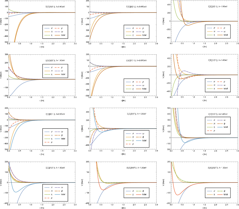
Figure 1: The interaction potentials for the two charmed baryons in the S-wave.

There are four candidates of $\Sigma_{c}^{*}\Sigma_{c}^{*}$ molecular states. For the $\Sigma_{c}^{*}\Sigma_{c}^{*}[0(2^{+})]$ system, the $\pi$ exchange potential is attractive when $r<1$ fm, which provides the main part of the total potential. The binding energy is 2.6-28.1 MeV when the cutoff parameter varies from 0.8 GeV to 0.9 GeV. For the $\Sigma_{c}^{*}\Sigma_{c}^{*}[2(0^{+})]$ system, $\pi$, $\eta$, $\rho$ and $\omega$ exchange potentials are considerably repulsive in the short-range and become attractive when $r>0.6$ fm. The $\sigma$ exchange potential is always attractive. As a result, the total potential is slightly attractive in the range $0.7<r<1.5$ fm. A bound state appears with binding energy about 2.3-11.1 MeV when the cutoff parameter is around 1.4-1.6 GeV. The potential of $\Sigma_{c}^{*}\Sigma_{c}^{*}[1(1^{+})]$ system is similar to that of $[0(2^{+})]$ system. The binding energy of the state is 18.8-55.6 MeV, while the cutoff parameter is 0.8-0.9 GeV. For the $\Sigma_{c}^{*}\Sigma_{c}^{*}[1(3^{+})]$ system, the total potential is repulsive when $r<0.3$ fm. In the range $0.4<r<1.5$ fm, the contributions of the $\rho$ and $\omega$ exchange cancel with each other significantly, which makes the total potential weakly attractive. As a result there exists a weak binding solution with the cutoff parameter is around 1.3-1.5 GeV.

The potentials of the $\Xi_{c}^{*}\Xi_{c}^{*}$ systems can be slightly attractive with an appropriate cutoff. For the $\Xi_{c}^{*}\Xi_{c}^{*}[0(1^{+})]$ system, the attractive potential arising from the one pion exchange leads to a binding solution. The binding energy is 10.3-85.9 MeV while the cutoff parameter is 0.85-0.95 GeV. For the $\Xi_{c}^{*}\Xi_{c}^{*}[0(3^{+})]$ systems, the $\pi$ and $\sigma$ exchange potentials are attractive around 0.5-1.0 fm. As a result, a slightly bound state with binding energy 2.1-11.0 MeV appears when the cutoff parameter is 1.1-1.3 GeV. For the $\Xi_{c}^{*}\Xi_{c}^{*}[1(0^{+}),1(2^{+})]$, the attractive parts of the potentials mainly come from the $\sigma$ exchange. The binding energy of the $\Xi_{c}^{*}\Xi_{c}^{*}[1(0^{+})]$ around 1.2-5.6 MeV with the cutoff is 1.3-1.5 GeV. The binding energy of the $\Xi_{c}^{*}\Xi_{c}^{*}[1(2^{+})]$ is 2.7-3.8 MeV when the cutoff varies from 1.1 GeV to 1.5 GeV.

For the $\Omega_{c}^{*}\Omega_{c}^{*}$ systems, two loosely bound states are obtained. There dose not exist the $\pi$ exchange between two $\Omega_{c}^{*}$s, which usually provides the main part of the total potential. Even so, the $\sigma$, $\eta$ and $\phi$ exchanges can also lead to a weakly attractive potential around 1 fm. For the $\Omega_{c}^{*}\Omega_{c}^{*}[0(0^{+})]$ system, we find a bound state with the binding energy about 2.4-6.0 MeV when the cutoff is 1.1-1.3 GeV. And for the $\Omega_{c}^{*}\Omega_{c}^{*}[0(2^{+})]$ system, a bound state with binding energy 5.2-11.8 MeV appears when the cutoff parameter is 1.0-1.4 GeV.

From the Fig. 1, one can notice that a strong attraction exists for the systems $\Sigma_{c}^{*}\Sigma_{c}^{*}[0(0^{+})]$ in the range $r<1$ fm. The strong attractive potential is provided by the $\pi$ exchange. The contribution of the other meson exchange is quite small. The strong attractive total potential generates a tightly bound system. We get a binding solution with very large binding energy and very small root-mean-square radius. The strong attraction in the channel strongly indicates that there may exist the heavy analogue of the H-dibaryon with the configurations such as ccqqqq where q denotes the up or down quark. For the system $\Sigma_{c}^{*}\Sigma_{c}^{*}[2(2^{+})]$, the total attractive potential is too weak to form a bound state. Actually we find no binding solution in a reasonable range for the cutoff parameter.

3.2 Couple Channel Calculation

Here, we consider the couple channel effect between states with different spin and angular momentum for comparison. These states are mixed by the tensor operator. For the system with spin 0, we consider the S-D wave mixing. For the system with spin 1, we add G-wave besides the S- and D-waves. For the D-wave channel, the spin of two baryons can be 1 or 3. The numerical results including the binding energy, root-mean-square radius and the percentages of different channels are shown in Table 5 and Table 6. The potentials of different channels are given in Figs. 2 and 3 respectively. There are three good candidates of molecular systems with total spin 0, $\Sigma_{c}^{*}\Sigma_{c}^{*}[2(0^{+})]$, $\Xi_{c}^{*}\Xi_{c}^{*}[1(0^{+})]$, and $\Omega_{c}^{*}\Omega_{c}^{*}[0(0^{+})]$. For the systems with total spin 1, the $\Sigma_{c}^{*}\Sigma_{c}^{*}[1(1^{+})]$ and $\Xi_{c}^{*}\Xi_{c}^{*}[0(1^{+})]$ are also good candidates of molecular states.

Table 5: The numerical results for two charmed baryons with total spin 0 in couple channel calculation. $\Lambda$ is the cutoff parameter. ”$E$” is the binding energy. $R_{rms}$ is the root-mean-square radius. We use $[I(J^{P})]$ to mark different states. $P_{S}$ is the percentage of the S wave, and $P_{D}$ is the percentage of the D wave.

States	$\Lambda$(MeV)	E(MeV)	$R_{rms}$(fm)	$P_{S}(\%)$	$P_{D}(\%)$	States	$\Lambda$(MeV)	E(MeV)	$R_{rms}$(fm)	$P_{S}(\%)$	$P_{D}(\%)$
$\Sigma_{c}^{*}\Sigma_{c}^{*}[0(0^{+})]$						$\Xi_{c}^{*}\Xi_{c}^{*}[1(0^{+})]$	1400	3.1	2.2	99.9	0.1
			$\times$				1600	11.5	1.4	99.6	0.4
							1800	27.8	1.1	98.8	1.2
$\Sigma_{c}^{*}\Sigma_{c}^{*}[2(0^{+})]$	1400	3.2	2.7	98.5	1.5	$\Omega_{c}^{*}\Omega_{c}^{*}[0(0^{+})]$	1000	2.1	2.5	98.5	1.5
	1500	7.5	2.0	99.0	0.1		1200	6.0	1.8	97.7	2.3
	1600	14.8	1.6	99.3	0.7		1400	11.3	1.5	99.5	0.5

Table 6: The numerical results for two charmed baryons with total spin 1 in couple channel calculation. $\Lambda$ is the cutoff parameter. ”$E$” is the binding energy. $R_{rms}$ is the root-mean-square radius. We use $[I(J^{P})]$ to mark different states. $P_{S}$ is the percentage of the ${}^{3}S_{1}$, $P_{D1}$ is the percentage of the ${}^{3}D_{1}$, $P_{D2}$ is the percentage of the ${}^{7}D_{1}$, and $P_{G}$ is the percentage of the ${}^{7}G_{1}$.

States	$\Lambda$(MeV)	E(MeV)	$R_{rms}$(fm)	$P_{S}(\%)$	$P_{D1}(\%)$	$P_{D2}(\%)$	$P_{G}(\%)$
$\Sigma_{c}^{*}\Sigma_{c}^{*}[1(1^{+})]$	800	23.3	1.1	98.1	1.5	0.4	0.0
	820	29.7	1.0	98.1	1.5	0.4	0.0
	840	36.8	0.9	98.2	1.4	0.4	0.0
$\Xi_{c}^{*^{\prime}}\Xi_{c}^{*^{\prime}}[0(1+)]$	820	4.9	1.9	97.4	2.0	0.6	0.0
	840	11.0	1.5	97.5	1.9	0.6	0.0
	860	19.6	1.2	97.9	1.6	0.5	0.0

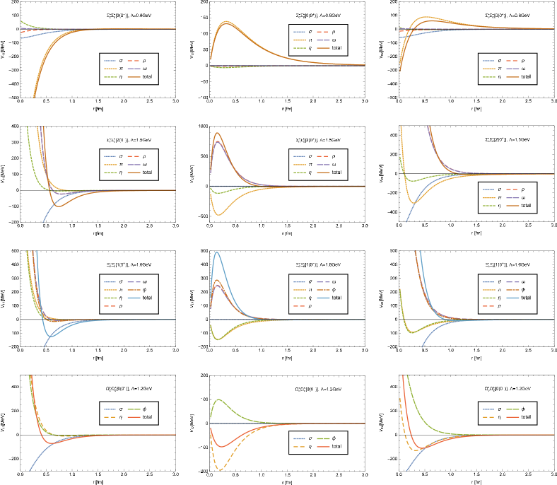
Figure 2: The interaction potentials for the two charmed baryons with total spin 0. Two channels are included. $V_{11},V_{12}$ and $V_{22}$ denote the ${}^{1}S_{0}\leftrightarrow{}^{1}S_{0}$, ${}^{1}S_{0}\leftrightarrow{}^{5}D_{0}$ and ${}^{5}D_{0}\leftrightarrow{}^{5}D_{0}$ transitions potentials. The four rows from top to bottom are for $\Sigma_{c}^{*}\Sigma_{c}^{*}[0(0^{+})],\Sigma_{c}^{*}\Sigma_{c}^{*}[2(0^{+})],\Xi_{c}^{*}\Xi_{c}^{*}[1(0^{+})]$ and $\Omega_{c}^{*}\Omega_{c}^{*}[0(0^{+})]$.

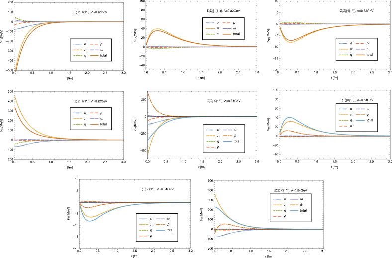
Figure 3: The interaction potentials for the $\Sigma_{c}^{*}\Sigma_{c}^{*}$ and $\Xi_{c}^{*}\Xi_{c}^{*}$ systems with total spin 1 in couple channel calculation. The subscript number “1-4” of “$V$” means states${}^{3}S_{1},{}^{3}D_{1},{}^{7}D_{1}$ and ${}^{7}G_{1}$ in sequence. We show only four representative potentials here. $V_{22}$ are similar to $V_{11}$. $V_{24}$ is similar to $V_{13}$. $V_{44}$ are similar to $V_{33}$.

For the $\Sigma_{c}^{*}\Sigma_{c}^{*}[2(0^{+})]$ system, one notices that the interaction potentials of the ${}^{5}D_{0}$ channel and the transition potential of ${}^{1}S_{0}\leftrightarrow{}^{5}D_{0}$ in Fig. 2 are both repulsive. There exists a loosely bound state with binding energy 3.2-14.8 MeV, while the cutoff is 1.4-1.6 GeV. The S-D mixing is quite small for the system. From Table 5, we notice that the probability of the D-wave is about 2%. For the $\Xi_{c}^{*}\Xi_{c}^{*}[1(0^{+})]$ and the $\Omega_{c}^{*}\Omega_{c}^{*}[0(0^{+})]$ systems, the S-D transition potentials both affect the solutions slightly. Their binding energies change slightly compared with the single channel cases. For the $\Sigma_{c}^{*}\Sigma_{c}^{*}[0(0^{+})]$ system, there is no slightly bound solution even if we consider the S-D wave mixing.

For the $\Sigma_{c}^{*}\Sigma_{c}^{*}[1(1^{+})]$ and $\Xi_{c}^{*}\Xi_{c}^{*}[0(1^{+})]$ systems with $J=1$, we can still find loosely bound solutions when the channel mixing effect is considered. Compared with the single channel cases, their binding energies become slightly larger, and more dependent on the cutoff parameter. We show their potentials in the Fig. 3.

4 DISCUSSIONS AND CONCLUSIONS

In this work, we have performed a systematic investigation of the possible deuteron-like molecules composed of a pair of spin-$\frac{3}{2}$ singly charmed baryons. We have calculated the single channel results for all possible states with different total spins, and considered the couple channel effect for total spin 0 and 1 systems. For the systems with total spin 0, the channel mixing is between ${}^{1}S_{0}$ and ${}^{5}D_{0}$. For the systems with total spin 1, we include four channels, ${}^{3}S_{1}$, ${}^{3}D_{1}$, ${}^{7}D_{1}$ and ${}^{7}G_{1}$ in calculation.

The hadronic molecule is assumed to be a loosely bound state of two color singlet components. The formation of the molecular state mainly arises from the relatively long range attraction, which can be described well in OBE model. However, the extremely short range interaction from the OBE model may be not very convincing. Therefore, the very deep binding solution arising from the strong short attraction may be not physical. Thus, according to an empirical and intuitive approach suggested in Ref. Li:2012bt , the binding energy of a molecular state formed by two charmed baryons is expected to be less than 240 MeV, and the root-mean-square radius to be larger than 0.6-1.0 fm. With the help of the criteria, we have used the binding energy and root-mean-square radius to make some educated guesses whether the system is a loosely bound state. We use $\times$ in the table of results to denote those systems with very large binding energies.

For the ten systems, $\Sigma_{c}^{*}\Sigma_{c}^{*}$$[0(2^{+})$, $2(0^{+})$, $1(1^{+})$, $1(3^{+})]$, $\Xi_{c}^{*}\Xi_{c}^{*}$$[0(1^{+})$, $0(3^{+})$, $1(0^{+})$, $1(2^{+})]$ and $\Omega_{c}^{*}\Omega_{c}^{*}$$[0(0^{+})$, $0(2^{+})]$, we have obtained loosely bound solutions with small binding energies and appropriate sizes. After we consider the channel mixing effect, the loosely binding solutions of the $\Sigma_{c}^{*}\Sigma_{c}^{*}[2(0^{+})]$, $[1(1^{+})]$, $\Xi_{c}^{*}\Xi_{c}^{*}[1(0^{+})]$, $[0(1^{+})]$, $\Omega_{c}^{*}\Omega_{c}^{*}$$[0(0^{+})]$ systems still exist. The multichannel effect always makes the binding slightly deeper. The cutoff parameters of the systems are almost in the range of 0.8-1.5 GeV, while that for the $\Sigma_{c}^{*}\Sigma_{c}^{*}$$[2(0^{+})]$ system is a little larger. Although the experience of the deuteron suggests a range from 0.8 GeV to 1.5 GeV, it may be reasonable to slightly widen the range for a much heavier system. Thus, they are all good molecular candidates. For the $\Sigma_{c}^{*}\Sigma_{c}^{*}[2(2^{+})]$ system, the potential is hardly attractive, and we find no binding solution with a reasonable cutoff parameter. For the $\Sigma_{c}^{*}\Sigma_{c}^{*}[0(0^{+})$ system, the OBE potential is strongly attractive, which indicates that the tightly bound heavy dibaryon may exist with the configurations such as ccssqq or ccqqqq where q denotes the up or down quark.

The mass difference between $\Omega_{c}^{*}$ and $\Omega_{c}$ is too small for any strong decay to occur. As a result, the $\Omega_{c}^{*}$ decays mainly via $\Omega_{c}^{*}\rightarrow\Omega_{c}\gamma$. Once the states are produced in experiments, they would be stable. Thus the $\Omega_{c}^{*}\Omega_{c}^{*}$ systems may be observed in the future.

We also calculate the systems formed by one baryon and one antibaryon in Appendix C. The present formalism can be extended easily to the loosely bound systems composed of two different spin-$\frac{3}{2}$ baryons, only by adding the influence of the $K$ and $K^{*}$ exchanges. The framework can be used to study the systems composed of one spin $\frac{1}{2}$-baryon and one spin-$\frac{3}{2}$ baryon. One may also extend the couple channel effect to the systems with different particles, such as $\Sigma_{c}^{*}\Sigma_{c}^{*}[0(0^{+})]\leftrightarrow\Sigma_{c}\Sigma_{c}[0(0^{+})]$.

Acknowledgements: BY is very grateful to X.Z Weng, H.S. Li and G.J. Wang for very helpful discussions. This project is supported by the National Natural Science Foundation of China under Grants 11575008, 11621131001 and National Key Basic Research Program of China (2015CB856700).

Appendix A Expressions of Special Functions and Some Fourier Transformation Formulae

The definitions of $H_{i}$ etc. are

$$\begin{split}H_{0}(\Lambda,m,r)&=Y(ur)-\frac{\lambda}{u}Y(\lambda r)-\frac{r\beta^{2}}{2u}Y(\lambda r),\\ H_{1}(\Lambda,m,r)&=Y(ur)-\frac{\lambda}{u}Y(\lambda r)-\frac{r\lambda^{2}\beta^{2}}{2u^{3}}Y(\lambda r),\\ H_{2}(\Lambda,m,r)&=Z_{1}(ur)-\frac{\lambda^{3}}{u^{3}}Z_{1}(\lambda r)-\frac{\lambda\beta^{2}}{2u^{3}}Y(\lambda r),\\ H_{3}(\Lambda,m,r)&=Z(ur)-\frac{\lambda^{3}}{u^{3}}Z(\lambda r)-\frac{\lambda\beta^{2}}{2u^{3}}Z_{2}(\lambda r),\\ M_{0}(\Lambda,m,r)&=-\frac{1}{\theta r}\left[\cos(\theta r)-e^{-\lambda r}\right]+\frac{\beta^{2}}{2\theta\lambda}e^{-\lambda r},\\ M_{1}(\Lambda,m,r)&=-\frac{1}{\theta r}\left[\cos(\theta r)-e^{-\lambda r}\right]-\frac{\lambda\beta^{2}}{2\theta^{3}}e^{-\lambda r},\\ M_{3}(\Lambda,m,r)&=-\left[\cos(\theta r)-\frac{3\sin(\theta r)}{\theta r}-3\frac{\cos(\theta r)}{\theta^{2}r^{2}}\right]\frac{1}{\theta r}\\ &~{}~{}~{}~{}-\frac{\lambda^{3}}{\theta^{3}}Z(\lambda r)-\frac{\lambda\beta^{2}}{2\theta^{3}}Z_{2}(\lambda r),\end{split}$$ (33)

where

$$\beta^{2}=\Lambda^{2}-m^{2},~{}~{}u^{2}=m^{2}-Q_{0}^{2},~{}~{}$$

$$\theta^{2}=-(m^{2}-Q_{0}^{2}),~{}~{}\lambda^{2}=\Lambda^{2}-Q_{0}^{2},$$

and

$$Y(x)=\frac{e^{-x}}{x},~{}~{}Z(x)=(1+\frac{3}{x}+\frac{3}{x^{2}})Y(x),$$

$$Z_{1}(x)=(\frac{1}{x}+\frac{1}{x^{2}})Y(x),~{}~{}Z_{2}(x)=(1+x)Y(x).$$

The parameter $Q_{0}$ is the zero component of the four momentum of exchanged meson.

We give some Fourier transformation formulae to derive the effective potential,

$$\begin{split}\frac{1}{u^{2}+\bm{Q}^{2}}\mathcal{F}^{2}(Q)&\rightarrow\frac{u}{4\pi}H_{0}(\Lambda,m,r),\\ \frac{\bm{Q}^{2}}{u^{2}+\bm{Q}^{2}}\mathcal{F}^{2}(Q)&\rightarrow-\frac{u^{3}}{4\pi}H_{1}(\Lambda,m,r),\\ \frac{\bm{Q}}{u^{2}+\bm{Q}^{2}}\mathcal{F}^{2}(Q)&\rightarrow\frac{iu^{3}}{4\pi}\bm{r}H_{2}(\Lambda,m,r),\\ \frac{Q_{i}Q_{j}}{u^{2}+\bm{Q}^{2}}\mathcal{F}^{2}(Q)&\rightarrow-\frac{u^{3}}{12\pi}\left[H_{3}(\Lambda,m,r)K_{ij}+H_{1}(\Lambda,m,r)\delta_{ij}\right].\end{split}$$ (34)

If $u_{ex}^{2}=m_{ex}^{2}-Q_{0}^{2}<0$, the last formula above changes into

$$\frac{Q_{i}Q_{j}}{u^{2}+\bm{Q}^{2}}\mathcal{F}^{2}(Q)\rightarrow-\frac{\theta^{3}}{12\pi}\left[M_{3}(\Lambda,m,r)K_{ij}+M_{1}(\Lambda,m,r)\delta_{ij}\right].$$

Appendix B Some Details of the Operators in the Lagrangian

We used some operators in the Eqs. (21-24),

$$\Delta_{S_{A}S_{B}}=\bm{\sigma}_{rsA}\cdot\bm{\sigma}_{rsB},\quad\Delta_{LS}={1\over 2}\bm{L}\cdot\bm{\sigma}_{rs},$$

$$\Delta_{T}={3\bm{\sigma}_{rsA}\cdot\bm{r}\bm{\sigma}_{rsB}\cdot\bm{r}\over r^{2}}-\bm{\sigma}_{rsA}\cdot\bm{\sigma}_{rsB}.$$ (35)

$\Delta_{S_{A}S_{B}}$, $\Delta_{LS}$ and $\Delta_{T}$ are spin-spin operator, spin-orbital operator and tensor operator, respectively. $\bm{\sigma}_{rs}$ is the spin operator for spin-$\frac{3}{2}$ baryons. $\bm{L}$ is the relative orbit angular momentum operator between the two baryons. $\bm{S}_{A}$ and $\bm{S}_{B}$ are the spin operators of two baryons respectively, while $\bm{S}=\bm{S}_{A}+\bm{S}_{B}$ is the total spin operator. For spin-$\frac{3}{2}$ baryons, $\bm{S}=\frac{3}{2}\bm{\sigma}_{rs}$.

We introduce the transition spin operator $S^{\mu}_{t}$ for the Rarita-Schwinger field $\Psi^{\mu}$, because we focus on the baryons with spin $\frac{3}{2}$. The field $\Psi^{\mu}$ can be expressed as

$$\Psi^{\mu}(\lambda)=\underset{m_{\lambda}}{\sum}\underset{m_{s}}{\sum}\epsilon^{\mu}(m_{\lambda})\chi(m_{s})=S^{\mu}_{t}\Phi,$$ (36)

where $\epsilon^{\mu}(m_{\lambda})$ is the polarization vector of a spin-1 field,

$$\begin{split}\epsilon^{\mu}(+)&=-\frac{1}{\sqrt{2}}\left[0,1,i,0\right]^{T},~{}\epsilon^{\mu}(0)=\left[0,0,0,1\right]^{T},\\ \epsilon^{\mu}(-)&=\frac{1}{\sqrt{2}}\left[0,1,-i,0\right]^{T}.\end{split}$$ (37)

$\chi$ is a two-component spinor. $\Phi$ is the spin wave function of spin $\frac{3}{2}$ baryons.

$$\begin{split}\Phi\left(\frac{3}{2}\right)&=\left[1,0,0,0\right]^{T},~{}\Phi\left(\frac{1}{2}\right)=\left[0,1,0,0\right]^{T},\\ \Phi\left(-\frac{1}{2}\right)&=\left[0,0,1,0\right]^{T},~{}\Phi\left(-\frac{3}{2}\right)=\left[0,0,0,1\right]^{T}.\end{split}$$ (38)

It is easy to obtain the transition spin operator,

$$\begin{split}S^{0}_{t}=&0,~{}S^{x}_{t}=\frac{1}{\sqrt{2}}\left[\begin{array}[]{cccc}-1&0&\frac{1}{\sqrt{2}}&0\\ 0&-\frac{1}{\sqrt{3}}&0&1\end{array}\right],\\ S^{y}_{t}=&-\frac{i}{\sqrt{2}}\left[\begin{array}[]{cccc}1&0&\frac{1}{\sqrt{3}}&0\\ 0&\frac{1}{\sqrt{3}}&0&1\end{array}\right],~{}S^{x}_{t}=\left[\begin{array}[]{cccc}0&\sqrt{\frac{2}{3}}&0&0\\ 0&0&\sqrt{\frac{2}{3}}&0\end{array}\right].\end{split}$$ (39)

The spin operator for spin-$3\over 2$ particles can be derived from the Pauli matrices $\bm{\sigma}_{rs}\equiv-S^{\dagger}_{t\mu}\bm{\sigma}S^{\mu}_{t}$. The explicit form is

$$\begin{split}\sigma_{rs}^{x}&=\left[\begin{array}[]{cccc}0&\frac{1}{\sqrt{3}}&0&0\\ \frac{1}{\sqrt{3}}&0&\frac{2}{3}&0\\ 0&\frac{2}{3}&0&\frac{1}{\sqrt{3}}\\ 0&0&\frac{1}{\sqrt{3}}&0\end{array}\right],~{}\sigma_{rs}^{y}=\left[\begin{array}[]{cccc}0&-\frac{i}{\sqrt{3}}&0&0\\ \frac{i}{\sqrt{3}}&0&-\frac{2i}{3}&0\\ 0&\frac{2i}{3}&0&-\frac{i}{\sqrt{3}}\\ 0&0&\frac{i}{\sqrt{3}}&0\end{array}\right],\\ \sigma_{rs}^{z}&=\left[\begin{array}[]{cccc}1&0&0&0\\ 0&\frac{1}{3}&0&0\\ 0&0&-\frac{1}{3}&0\\ 0&0&0&-1\end{array}\right]\end{split}$$ (40)

The tensor operator $\Delta_{T}$ is actually a scalar product of two rank-2 tensor operators, $Y_{2,m}(\hat{r})$ and $T_{2,m}$

$$\Delta_{T}=\overset{2}{\underset{m=-2}{\sum}}4\sqrt{\frac{6\pi}{5}}T_{2,m}Y_{2,m}^{*}(\hat{r})$$ (41)

The operator $Y_{2,m}(\hat{r})$ is the spherical harmonic function, and $T_{2,m}$ is a rank-2 tensor operator constructed by spin operator

$$\begin{split}&T_{2,\pm 2}=\frac{3}{8\pi}(S_{x}\pm iS_{y})^{2},\\ &T_{2,\pm 1}=\mp\frac{3}{8\pi}[S_{z}(S_{x}\pm iS_{y})+(S_{x}\pm iS_{y})S_{z}],\\ &T_{2,0}=\frac{3}{4\sqrt{6}\pi}(3S_{z}^{2}-\bm{S}^{2}).\end{split}$$ (42)

We can get the expression of the matrix elements of the tensor operator

$$\begin{split}&\braket{L_{f}S_{f}J_{f}m_{f}}{\Delta_{T}}{L_{i}S_{i}J_{i}m_{i}}\\ =&\underset{m_{1}}{\sum}\underset{m_{2}}{\sum}\underset{m_{3}}{\sum}\underset{m_{4}}{\sum}\braket{L_{f}\left[m_{f}-(m_{3}+m_{4})\right],S_{f}(m_{3}+m_{4})}{J_{f}m_{f}}\\ &\times\braket{L_{i}\left[m_{i}-(m_{1}+m_{2})\right],S_{f}(m_{3}+m_{4})}\\ &\times\braket{\frac{3}{2}m_{3},\frac{3}{2}m_{4}}{S_{f}(m_{3}+m_{4})}\braket{\frac{3}{2}m_{1},\frac{3}{2}m_{2}}{S_{i}(m_{1}+m_{2})}\\ &\times\int^{2\pi}_{0}d\phi\int_{0}^{\pi}\sin(\theta)d\theta Y^{*}_{L_{f},m_{f}-(m_{3}+m_{4})}Y_{L_{i},m_{i}-(m_{1}+m_{2})}\\ &\times\bigg{[}3\braket{\frac{3}{2}m_{3}}{\vec{\sigma}_{rs1}}{\frac{3}{2}m_{1}}\cdot\hat{r}(\theta,\phi)\braket{\frac{3}{2}m_{4}}{\vec{\sigma}_{rs2}}{\frac{3}{2}m_{2}}\cdot\hat{r}(\theta,\phi)\\ &-\braket{\frac{3}{2}m_{3}}{\vec{\sigma}_{rs1}}{\frac{3}{2}m_{1}}\cdot\braket{\frac{3}{2}m_{4}}{\vec{\sigma}_{rs2}}{\frac{3}{2}m_{2}}\bigg{]}.\end{split}$$ (43)

The matrix elements of the tensor operator is independent of $m_{i}$ and $m_{f}$ according to the Wigner-Eckart theorem.

Appendix C Numerical Results of Baryon-antibaryon Systems

We calculate the possible molecular states formed by one baryon and one antibaryon. In this section we perform the single channel calculation for baryon-antibaryon systems first. And then we take the multichannel effects for $J=0$ and $J=1$ systems. In this section, we only take the one-boson-exchange interaction into consideration. In fact, the three meson threshold may have a significant influence on the baryon-antibaryon systems. The threshold may change the existence or properties of the possible molecular states we obtained. Some of the binding solutions we obtained for the baryon-antibaryon systems may be narrow molecule-type resonances like X(3872).

C.1 Single Channel Calculation

The numerical results of the baryon-antibaryon systems are collected in Table 7. The relevant potentials are shown in Fig. 4. We find some candidates of molecular states when the cutoff parameters are suitable.

Table 7: The numerical results for baryon-antibaryon single channel systems. $\Lambda$ is the cutoff parameter. ”$E$” is the binding energy. $R_{rms}$ is the root-mean-square radius. We use $[I(J^{P})]$ to mark different states.

States	$\Lambda$(MeV)	E(MeV)	$R_{rms}$(fm)	States	$\Lambda$(MeV)	E(MeV)	$R_{rms}$(fm)
$\Sigma_{c}^{*}\bar{\Sigma}_{c}^{*}[0(0^{-})]$	1040	13.9	1.0	$\Xi_{c}^{*}\bar{\Xi}_{c}^{*}[0(0^{-})]$	1000	0.4	4.4
	1060	76.0	0.5		1050	10.4	1.2
	1080	185.2	0.4		1100	56.3	0.6
$\Sigma_{c}^{*}\bar{\Sigma}_{c}^{*}[0(1^{-})]$	1020	5.7	1.6	$\Xi_{c}^{*}\bar{\Xi}_{c}^{*}[0(1^{-})]$	1000	2.5	2.2
	1040	23.6	0.9		1050	15.2	1.0
	1060	62.2	0.6		1100	49.9	0.6
$\Sigma_{c}^{*}\bar{\Sigma}_{c}^{*}[0(2^{-})]$	950	6.6	1.5	$\Xi_{c}^{*}\bar{\Xi}_{c}^{*}[0(2^{-})]$	950	4.5	1.7
	1000	25.6	0.9		1000	12.8	1.2
	1050	58.3	0.7		1050	26.4	0.9
$\Sigma_{c}^{*}\bar{\Sigma}_{c}^{*}[0(3^{-})]$	1000	103.6	0.6	$\Xi_{c}^{*}\bar{\Xi}_{c}^{*}[0(3^{-})]$	800	4.7	1.6
	1100	111.8	0.7		900	21.1	0.9
	1200	139.6	0.7		1000	39.2	0.8
$\Sigma_{c}^{*}\bar{\Sigma}_{c}^{*}[1(0^{-})]$	1000	6.0	1.5	$\Xi_{c}^{*}\bar{\Xi}_{c}^{*}[1(0^{-})]$	800	23.0	0.8
	1020	24.1	0.8		900	11.1	1.1
	1040	60.4	0.6		1000	18.6	1.0
$\Sigma_{c}^{*}\bar{\Sigma}_{c}^{*}[1(1^{-})]$	980	3.4	2.0	$\Xi_{c}^{*}\bar{\Xi}_{c}^{*}[1(1^{-})]$	800	10.3	1.1
	1000	10.8	1.2		900	7.1	1.4
	1020	25.4	0.9		1000	15.1	1.0
$\Sigma_{c}^{*}\bar{\Sigma}_{c}^{*}[1(2^{-})]$	950	7.2	1.5	$\Xi_{c}^{*}\bar{\Xi}_{c}^{*}[1(2^{-})]$	900	2.1	2.3
	1000	22.9	1.0		1000	9.2	1.3
	1050	47.9	0.7		1100	24.3	0.9
$\Sigma_{c}^{*}\bar{\Sigma}_{c}^{*}[1(3^{-})]$	800	13.9	1.0	$\Xi_{c}^{*}\bar{\Xi}_{c}^{*}[1(3^{-})]$	1000	3.2	1.9
	900	33.6	0.8		1100	12.3	1.1
	1000	45.3	0.8		1200	23.6	0.9
$\Sigma_{c}^{*}\bar{\Sigma}_{c}^{*}[2(0^{-})]$	800	41.1	0.7	$\Omega_{c}^{*}\bar{\Omega}_{c}^{*}[0(0^{-})]$	1000	0.8	3.5
	850	62.4	0.6		1100	4.6	1.8
	900	88.3	0.5		1200	25.5	0.9
$\Sigma_{c}^{*}\bar{\Sigma}_{c}^{*}[2(1^{-})]$	800	18.0	1.0	$\Omega_{c}^{*}\bar{\Omega}_{c}^{*}[0(1^{-})]$	1000	1.4	2.8
	850	31.6	0.8		1100	6.8	1.5
	900	49.0	0.7		1200	31.7	0.8
$\Sigma_{c}^{*}\bar{\Sigma}_{c}^{*}[2(2^{-})]$	900	4.4	1.7	$\Omega_{c}^{*}\bar{\Omega}_{c}^{*}[0(2^{-})]$	900	4.2	1.7
	1000	18.2	1.0		1000	5.3	1.6
	1100	39.6	0.7		1100	17.4	1.0
$\Sigma_{c}^{*}\bar{\Sigma}_{c}^{*}[2(3^{-})]$	1300	2.5	2.3	$\Omega_{c}^{*}\bar{\Omega}_{c}^{*}[0(3^{-})]$	800	4.1	1.9
	1400	5.4	1.7		900	4.9	1.6
	1500	9.1	1.4		1000	34.2	0.7

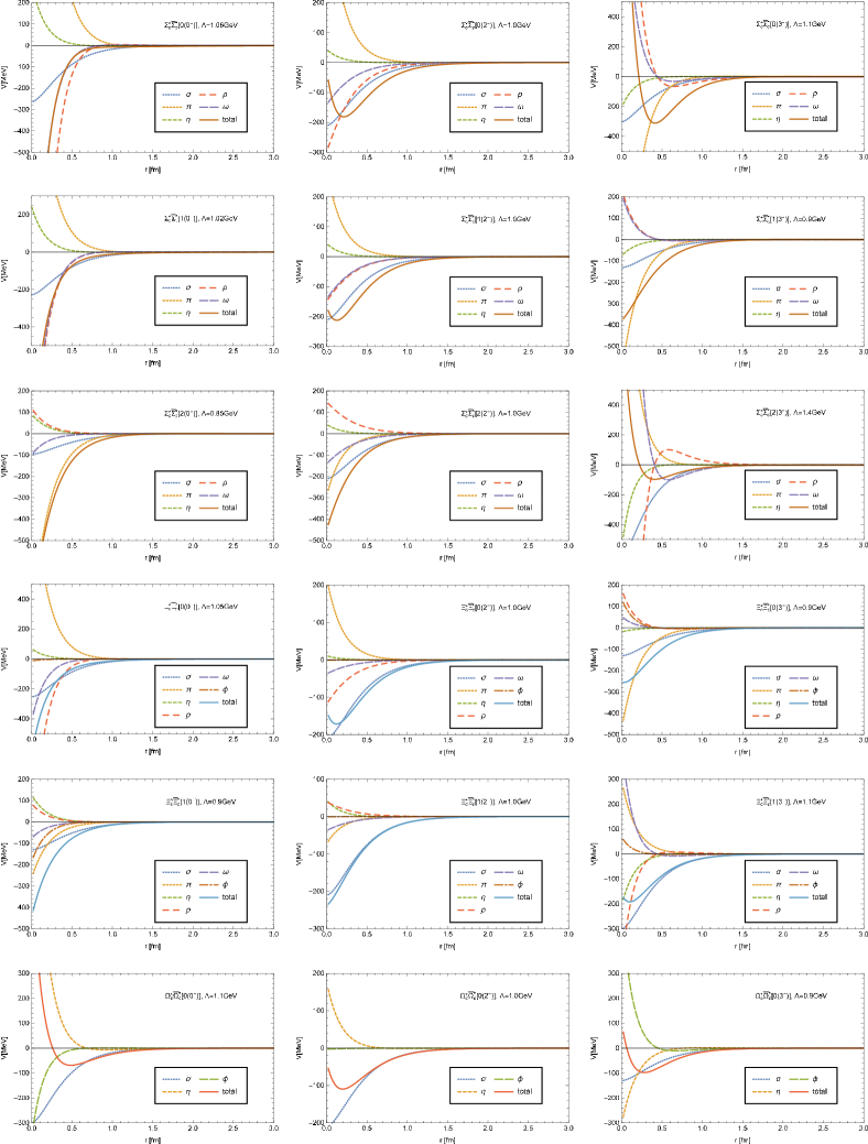
Figure 4: The interaction potentials for the baryon-antibaryon single channel systems.

For the $\Sigma_{c}^{*}\bar{\Sigma}_{c}^{*}$ system, the potential arises from the $\sigma$, $\pi$, $\eta$, $\rho$ and $\omega$ exchanges. They are all candidates of molecular states when some suitable cutoff parameters are chosen. We find binding solutions for the $\Sigma_{c}^{*}\bar{\Sigma}_{c}^{*}[0(0^{-})$, $0(1^{-})$, $1(0^{-})]$ systems, when the cutoff parameters are around 1.0 GeV. The solutions are more dependent on the cutoff than other systems. For the $\Sigma_{c}^{*}\bar{\Sigma}_{c}^{*}[0(3^{-})]$ system, we find a solution with binding energy 103.6-139.6 MeV, when the cutoff parameter varies from 1.0 GeV to 1.2 GeV. The binding energy is less dependent on the cutoff. For the $\Sigma_{c}^{*}\bar{\Sigma}_{c}^{*}[1(2^{-})]$ system, the $\sigma$, $\rho$ and $\omega$ exchange potentials are attractive, while the $\pi$, $\eta$ exchange potentials are weakly repulsive. We find a molecular solution with the binding energy 7.2-47.9 MeV when the cutoff parameter is from 0.95 GeV to 1.05 GeV. For the $\Sigma_{c}^{*}\bar{\Sigma}_{c}^{*}[2(0^{-})]$ system, the $\pi$ exchange is dominant, which is repulsive in the range $r<1$ fm. The binding energy is 41.1-88.3 MeV when the cutoff parameter is 0.8-0.9 GeV. For the $\Sigma_{c}^{*}\bar{\Sigma}_{c}^{*}[2(3^{-})]$ system, the contributions of the $\rho$ and $\omega$ exchanges cancel out. The contributions from other mesons make the total potential slightly attractive. As a result, we find a binding solution with a small binding energy, 2.5-9.1 MeV, when the cutoff parameter is 1.3-1.5 GeV.

For the $\Xi_{c}^{*}\bar{\Xi}_{c}^{*}$ systems, we get some loosely binding solutions when the cutoff is about 1 GeV. They are candidates of molecular states. Compared with the $\Sigma_{c}^{*}\bar{\Sigma}_{c}^{*}$ systems, the $\Xi_{c}^{*}\bar{\Xi}_{c}^{*}$ system also allows the $\phi$ meson exchange, although it’s contribution is usually small. For the $\Xi_{c}^{*}\bar{\Xi}_{c}^{*}[0(0^{-})$, $0(1^{-})$, $0(2^{-})]$ systems, the $\pi$ exchange provides the repulsive part of the total potential. The attractive part mainly arises from the $\sigma$, $\rho$ and $\omega$ exchanges. Their binding energies and $R_{rms}$ are shown in Table7. For the $\Xi_{c}^{*}\bar{\Xi}_{c}^{*}[0(1^{-})]$ system, the $\pi$ and $\sigma$ exchange provide the weakly attractive potential. The binding energy is 4.7-39.2 MeV with the cutoff parameter from 0.8 GeV to 1.0 GeV. For the $\Xi_{c}^{*}\bar{\Xi}_{c}^{*}[1(2^{-})]$ system, the attractive potential mainly comes from the $\sigma$ exchange. A molecular solution with the binding energy 2.1-24.3 MeV appears when the cutoff is 0.9-1.1 GeV. For the $\Xi_{c}^{*}\bar{\Xi}_{c}^{*}[1(3^{-})]$ system. We get the numerical result with the binding energy 3.2-23.6 MeV, when the cutoff parameter varies form 1.0 GeV to 1.2 GeV.

For the $\Omega_{c}^{*}\bar{\Omega}_{c}^{*}$ systems with spin 0,1,2, we get some deuteron-like solutions. All the $\Omega_{c}^{*}\bar{\Omega}_{c}^{*}$ systems are expected to be candidates of molecular states. From the Fig. 4, it seems that $\sigma$ exchange provides most of the potential. The total potential is weakly attractive in the medium and long range. The binding energy of $\Omega_{c}^{*}\bar{\Omega}_{c}^{*}[0(0^{-})]$ is 0.8-25.5 MeV when the cutoff is from 1.0 GeV to 1.2 GeV. The binding energy of $\Omega_{c}^{*}\bar{\Omega}_{c}^{*}[0(1^{-})]$ is 1.4-31.7 MeV when the cutoff parameter is in the range of 1.0 GeV-1.2 GeV. For the $\Omega_{c}^{*}\bar{\Omega}_{c}^{*}[0(2^{-})]$, the binding energy is 4.2-17.4 MeV when the cutoff parameter changes from 0.9 GeV to 1.1 GeV. For the $\Omega_{c}^{*}\bar{\Omega}_{c}^{*}[0(3^{-})]$, the main part of the potential comes from the $\sigma$ and $\eta$ exchanges. The binding energy is 4.1-34.2 MeV when the cutoff is from 0.8 GeV to 1.0 GeV.

C.2 Couple Channel Calculation

In this subsection, the couple channel effect is added for $J=0,1$ systems. The numerical results are shown in Tables 8 and 9 respectively. The corresponding potentials are given in Figs. 5-7.

Table 8: The numerical results for two baryon-antibaryon couple channel systems with total spin 0. $\Lambda$ is the cutoff parameter. ”$E$” is the binding energy. $R_{rms}$ is the root-mean-square radius. We use $[I(J^{P})]$ to mark different states. $P_{S}$ is the percentage of the S wave, and $P_{D}$ is the percentage of the D wave.

States	$\Lambda$(MeV)	E(MeV)	$R_{rms}$(fm)	$P_{S}(\%)$	$P_{D}(\%)$	States	$\Lambda$(MeV)	E(MeV)	$R_{rms}$(fm)	$P_{S}(\%)$	$P_{D}(\%)$
$\Sigma_{c}^{*}\bar{\Sigma}_{c}^{*}[0(0^{-})]$	800	5.1	3.0	71.7	28.3	$\Xi_{c}^{*}\bar{\Xi}_{c}^{*}[0(0^{-})]$	950	5.5	2.2	86.8	13.2
	850	14.9	2.1	60.9	39.1		1000	21.4	1.4	80.5	19.5
	900	43.8	1.5	50.6	49.4		1050	61.1	1.0	77.4	22.6
$\Sigma_{c}^{*}\bar{\Sigma}_{c}^{*}[1(0^{-})]$	900	4.2	2.6	83.1	16.9	$\Xi_{c}^{*}\bar{\Xi}_{c}^{*}[1(0^{-})]$	900	11.2	1.2	99.9	0.1
	920	9.9	2.0	77.3	22.7		1000	18.9	1.0	99.8	0.2
	940	20.1	1.6	72.5	27.5		1100	40.9	0.8	99.9	0.1
$\Sigma_{c}^{*}\bar{\Sigma}_{c}^{*}[2(0^{-})]$	800	45.6	0.8	98.7	1.3	$\Omega_{c}^{*}\bar{\Omega}_{c}^{*}[0(0^{-})]$	900	7.8	1.5	97.1	2.9
	850	67.9	0.7	98.7	1.3		1000	2.3	2.4	98.3	1.7
	900	94.9	0.6	98.8	1.2		1100	13.2	1.4	93.5	6.5

Table 9: The numerical results for two baryon-antibaryon couple channel systems with total spin 1. $\Lambda$ is the cutoff parameter. ”$E$” is the binding energy. $R_{rms}$ is the root-mean-square radius. We use $[I(J^{P})]$ to mark different states. $P_{S}$ is the percentage of the ${}^{3}S_{1}$, $P_{D1}$ is the percentage of the ${}^{3}D_{1}$, $P_{D2}$ is the percentage of the ${}^{7}D_{1}$, and $P_{G}$ is the percentage of the ${}^{7}G_{1}$.

States	$\Lambda$(MeV)	E(MeV)	$R_{rms}$(fm)	$P_{S}(\%)$	$P_{D1}(\%)$	$P_{D2}(\%)$	$P_{G}(\%)$
$\Sigma_{c}^{*}\bar{\Sigma}_{c}^{*}[0(1^{-})]$	800	5.1	3.3	72.0	13.1	14.8	0.1
	820	8.2	2.9	67.1	14.0	18.7	0.2
	840	13.5	2.6	61.6	14.5	23.7	0.2
$\Sigma_{c}^{*}\bar{\Sigma}_{c}^{*}[1(1^{-})]$	880	1.9	3.5	89.2	5.7	5.1	0.0
	900	5.4	2.6	83.8	7.8	8.3	0.1
	940	22.8	1.8	74.2	10.1	15.6	0.1
$\Sigma_{c}^{*}\bar{\Sigma}_{c}^{*}[2(1^{-})]$	800	22.6	1.1	98.0	1.5	0.5	0.0
	820	28.1	1.0	98.1	1.5	0.4	0.0
	840	34.2	1.0	98.1	1.5	0.4	0.0
$\Xi_{c}^{*^{\prime}}\bar{\Xi}_{c}^{*^{\prime}}[0(1^{-})]$	900	1.5	3.5	93.4	3.7	2.9	0.0
	950	7.5	2.1	88.0	6.1	5.9	0.0
	1000	24.2	1.5	82.9	7.7	9.4	0.0
$\Xi_{c}^{*^{\prime}}\bar{\Xi}_{c}^{*^{\prime}}[1(1^{-})]$	800	10.4	1.2	100.0	0.0	0.0	0.0
	900	7.2	1.4	99.9	0.1	0.0	0.0
	1000	15.4	1.1	99.8	0.1	0.1	0.0
$\Omega_{c}^{*}\bar{\Omega}_{c}^{*}[0(1^{-})]$	900	7.4	1.6	97.5	1.5	1.0	0.0
	1000	3.2	2.2	98.3	1.1	0.6	0.0
	1100	15.8	1.4	94.2	3.5	2.3	0.0

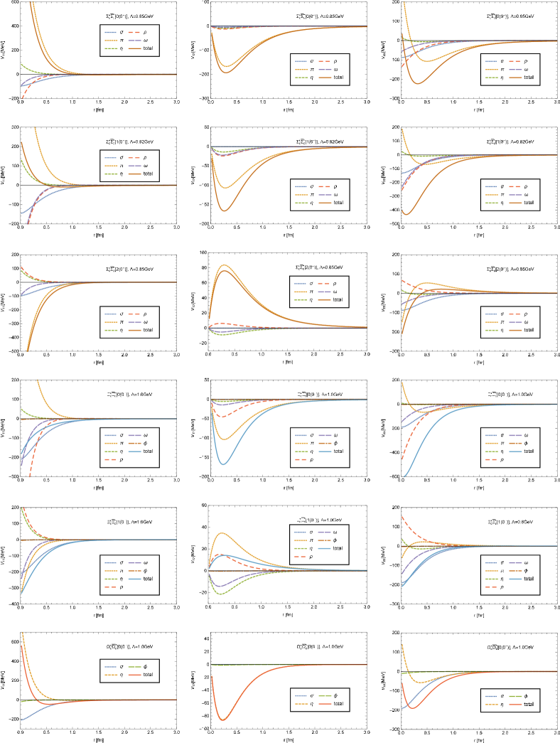
Figure 5: Some typical interaction potentials for the baryon-antibaryon couple channel systems with total spin 0. $V_{11},V_{12}$ and $V_{22}$ denote the ${}^{1}S_{0}\leftrightarrow{}^{1}S_{0},{}^{1}S_{0}\leftrightarrow{}^{5}D_{0}$ and ${}^{5}D_{0}\leftrightarrow{}^{5}D_{0}$ transitions potentials.

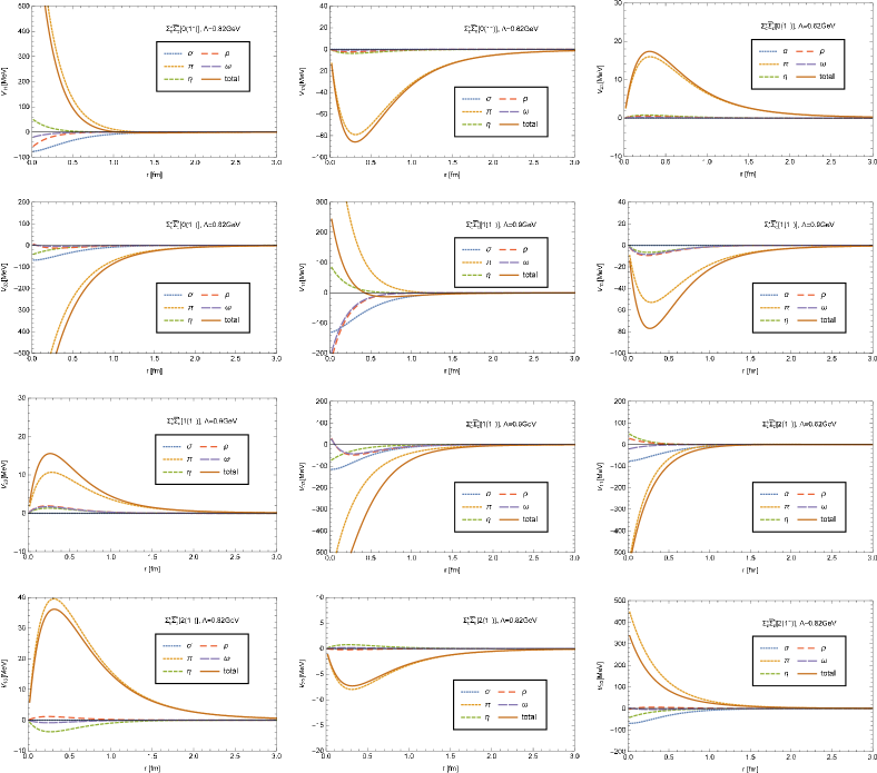
Figure 6: Some typical interaction potentials for the $\Sigma_{c}^{*}\bar{\Sigma}_{c}^{*}$ couple channel systems with total spin 1. The subscript number 1-4 means states${}^{3}S_{1},{}^{3}D_{1},{}^{7}D_{1}$ and ${}^{7}G_{1}$ in sequence. We put only four representative potentials here. For other potentials, $V_{12}$ and $V_{22}$ are similar to $V_{11}$, $V_{24}$ is similar to $V_{13}$, while $V_{34}$ and $V_{44}$ are similar to $V_{34}$.

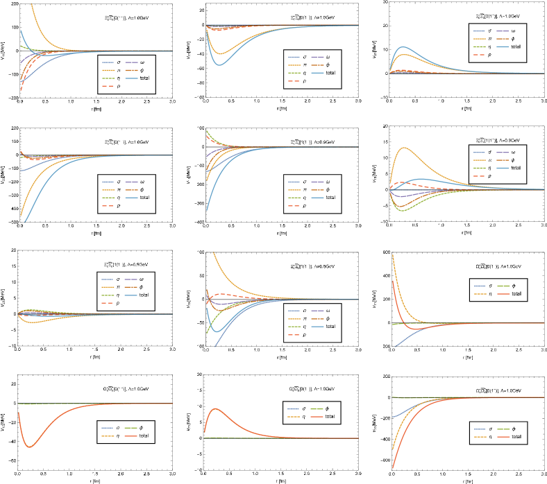
Figure 7: Some typical interaction potentials for the $\Xi_{c}^{*}\bar{\Xi}_{c}^{*}$ and $\Omega_{c}^{*}\bar{\Omega}_{c}^{*}$ couple channel systems with total spin 1. The subscript number 1-4 means states${}^{3}S_{1},{}^{3}D_{1},{}^{7}D_{1}$ and ${}^{7}G_{1}$ in sequence. We put only four representative potentials here. For other potentials, $V_{12}$ and $V_{22}$ are similar to $V_{11}$, $V_{24}$ is similar to $V_{13}$, while $V_{34}$ and $V_{44}$ are similar to $V_{34}$.

For the states with total spin 0, we consider the couple channel effect for the six systems, $\Sigma_{c}^{*}\bar{\Sigma}_{c}^{*}$ with isospin 0, 1, 2, and $\Xi_{c}^{*}\bar{\Xi}_{c}^{*}$ with isospin 0, 1 as well as $\Omega_{c}^{*}\bar{\Omega}_{c}^{*}[0(0^{-})]$. They are all candidates of molecular states. For most cases, the D-wave channel affects the S-wave channel slightly. For the $\Xi_{c}^{*}\bar{\Xi}_{c}^{*}[1(0^{-})]$ system, as shown in Table 8, the D-wave contribution in the total wave function is about 0.1%, and makes the binding energy shift 0.2 MeV when the cutoff parameter is 0.9 GeV. The $\Sigma_{c}^{*}\bar{\Sigma}_{c}^{*}$$[0(0^{-})]$ system is interesting. The couple channel effect does change the result quite a lot. The D-wave contribution is around 40%. For the single channel case, we choose the cutoff parameter from 1.04 GeV to 1.06 GeV. After considering the couple channel effect, we choose a new range of cutoff parameter, 0.8-0.9 GeV, to get the binding solutions with reasonable small binding energies, 5.1-43.8 MeV. For the $\Sigma_{c}^{*}\bar{\Sigma}_{c}^{*}[1(0^{-})]$ system, we find a loosely bound solution, whose binding energy is 4.2-20.1 MeV, when the cutoff parameter is 0.9-0.94 GeV. The couple channel effect also has a significant influence on the system. For the $\Sigma_{c}^{*}\bar{\Sigma}_{c}^{*}[2(0^{-})]$ system, the couple channel effect only makes the binding a little deeper. For the $\Xi_{c}^{*}\bar{\Xi}_{c}^{*}[0(0^{-})]$ system, the binding energy is 5.5-61.1 MeV while the cutoff parameter is 0.95-1.05 MeV. For the $\Omega_{c}^{*}\bar{\Omega}_{c}^{*}[0(0^{-})]$ system, a molecular solution appears when the cutoff parameter varies from 0.9 GeV to 1.1 GeV.

For the system with spin 1, we add G-wave besides the S- and D-waves. All the six systems are candidates of molecular states. For the $\Sigma_{c}^{*}\bar{\Sigma}_{c}^{*}[0(1^{-})]$ system, the D-waves have a nontrivial influence. The contribution of D-waves is almost 40%, when the cutoff is 0.84 GeV. The large D-waves contribution makes us choose the different cutoff parameters from the single channel case. The binding energy for multichannel calculation is 5.1-13.5 MeV, while the cutoff parameter is 0.8-0.84 GeV. For the $\Sigma_{c}^{*}\bar{\Sigma}_{c}^{*}[1(1^{-})]$ system, the effect of D-waves is also obvious. The binding energy is 1.9-22.8 MeV when the cutoff is 8.8-9.4 GeV. The $\Xi_{c}^{*}\bar{\Xi}_{c}^{*}[0(1^{-})]$ system is similiar. We find that a loosely binding solution with binding energy 1.5-24.2 MeV appears when the cutoff parameter is 0.9-1.0 GeV. For the $\Sigma_{c}^{*}\bar{\Sigma}_{c}^{*}[1(1^{-})]$ system, the S-wave dominates the total wave function. The binding energy is larger than the single channel calculation. For the $\Xi_{c}^{*}\bar{\Xi}_{c}^{*}[1(1^{-})]$ system, the D-wave contribution is less than 0.2%, the binding energy is also larger than that in the single channel case. For the $\Omega_{c}^{*}\bar{\Omega}_{c}^{*}[0(1^{-})]$ state, the couple channel effect makes the binding deeper as expected. The binding energy is 3.2 MeV while the cutoff is 1.0 GeV.

C.3 Summary

We calculate the baryon-antibaryon systems with different spin and isospin in single channel, and find the loosely bound solutions. After considering the channel mixing effect, we calculate the systems with total spin 0 and 1. For the most systems, the multichannel effect would lead to a deeper binding solution. For the $\Sigma_{c}^{*}\bar{\Sigma}_{c}^{*}$$[0(0^{-})$, $1(0^{-})$, $0(1^{-})$, $1(1^{-})]$ and $\Xi_{c}^{*}\Xi_{c}^{*}$$[0(1-)]$ systems, the D-wave contribution is nontrivial, and may even reaches up to 40%.

Moreover, a baryon-antibaryon molecular state may also decay into three mesons through quark rearrangement, which makes the molecular states unstable. Some of the “bound sates” obtained in this section may appear as other structures in experiment considering the open three mesons threshold. On the one hand, some of these binding solutions may appear as a possible enhancement of the baryon and antibaryon invariant mass spectrum in experiment, instead of as a real resonance. On the other hand, some of these binding solutions may appear as a narrow resonance state like X(3872). X(3872) is a good candidate of the $D\bar{D}^{*}$ molecule. Although it decays into $D\bar{D}\pi$, X(3872) is still a very narrow resonance. Another example, the charged $Z_{c}$ states containing four quarks, are above some two mesons thresholds. Even though the $Z_{c}$ states decay into two mesons through quark rearrangement, they still appear as rather narrow resonances in experiment.

References

• (1) S. K. Choi et al. [Belle Collaboration], Phys. Rev. Lett.  91, 262001 (2003)
• (2) B. Aubert et al. [BaBar Collaboration], Phys. Rev. Lett.  95, 142001 (2005)
• (3) Z. Q. Liu et al. [Belle Collaboration], Phys. Rev. Lett.  110, 252002 (2013)
• (4) M. Ablikim et al. [BESIII Collaboration], Phys. Rev. Lett.  110, 252001 (2013)
• (5) A. Bondar et al. [Belle Collaboration], Phys. Rev. Lett.  108, 122001 (2012)
• (6) R. Aaij et al. [LHCb Collaboration], Phys. Rev. Lett.  115, 072001 (2015)
• (7) H. X. Chen, W. Chen, X. Liu and S. L. Zhu, Phys. Rept.  639, 1 (2016)
• (8) A. Esposito, A. Pilloni and A. D. Polosa, Phys. Rept.  668, 1 (2016)
• (9) H. X. Chen, W. Chen, X. Liu, Y. R. Liu and S. L. Zhu, Rept. Prog. Phys.  80, no. 7, 076201 (2017)
• (10) R. F. Lebed, R. E. Mitchell and E. S. Swanson, Prog. Part. Nucl. Phys.  93, 143 (2017)
• (11) F. K. Guo, C. Hanhart, U. G. Meissner, Q. Wang, Q. Zhao and B. S. Zou, Rev. Mod. Phys.  90, no. 1, 015004 (2018)
• (12) S. L. Olsen, T. Skwarnicki and D. Zieminska, Rev. Mod. Phys.  90, no. 1, 015003 (2018)
• (13) M. B. Voloshin and L. B. Okun, JETP Lett.  23, 333 (1976)
• (14) A. De Rujula, H. Georgi and S. L. Glashow, Phys. Rev. Lett.  38, 317 (1977).
• (15) N. A. Tornqvist, Z. Phys. C 61, 525 (1994)
• (16) N. A. Tornqvist, Nuovo Cim. A 107, 2471 (1994)
• (17) C. Y. Wong, Phys. Rev. C 69, 055202 (2004)
• (18) X. Liu and S. L. Zhu, Phys. Rev. D 80, 017502 (2009) Erratum: [Phys. Rev. D 85, 019902 (2012)]
• (19) F. Close and C. Downum, Phys. Rev. Lett.  102, 242003 (2009)
• (20) G. J. Ding, J. F. Liu and M. L. Yan, Phys. Rev. D 79, 054005 (2009)
• (21) Z. F. Sun, J. He, X. Liu, Z. G. Luo and S. L. Zhu, Phys. Rev. D 84, 054002 (2011)
• (22) N. Li, Z. F. Sun, X. Liu and S. L. Zhu, Phys. Rev. D 88, no. 11, 114008 (2013)
• (23) L. Zhao, L. Ma and S. L. Zhu, Phys. Rev. D 89, no. 9, 094026 (2014)
• (24) N. Lee, Z. G. Luo, X. L. Chen and S. L. Zhu, Phys. Rev. D 84, 014031 (2011)
• (25) W. Meguro, Y. R. Liu and M. Oka, Phys. Lett. B 704, 547 (2011)
• (26) N. Li and S. L. Zhu, Phys. Rev. D 86, 014020 (2012)
• (27) L. Meng, N. Li and S. L. Zhu, Phys. Rev. D 95, no. 11, 114019 (2017)
• (28) L. Meng, N. Li and S. l. Zhu, Eur. Phys. J. A 54, no. 9, 143 (2018)
• (29) J. Vijande, A. Valcarce, J. M. Richard and P. Sorba, Phys. Rev. D 94, no. 3, 034038 (2016)
• (30) T. F. Carames and A. Valcarce, Phys. Rev. D 92, no. 3, 034015 (2015)
• (31) N. Kaiser, P. B. Siegel and W. Weise, Phys. Lett. B 362, 23 (1995)
• (32) J. A. Oller and U. G. Meissner, Phys. Lett. B 500, 263 (2001)
• (33) K. P. Khemchandani, H. Kaneko, H. Nagahiro and A. Hosaka, Phys. Rev. D 83, 114041 (2011)
• (34) J. X. Lu, Y. Zhou, H. X. Chen, J. J. Xie and L. S. Geng, Phys. Rev. D 92, no. 1, 014036 (2015)
• (35) G. Montaña, A. Feijoo and À. Ramos, Eur. Phys. J. A 54, no. 4, 64 (2018)
• (36) W. H. Liang, J. M. Dias, V. R. Debastiani and E. Oset, Nucl. Phys. B 930, 524 (2018)
• (37) J. J. Wu, R. Molina, E. Oset and B. S. Zou, Phys. Rev. Lett.  105, 232001 (2010)
• (38) Z. C. Yang, Z. F. Sun, J. He, X. Liu and S. L. Zhu, Chin. Phys. C 36, 6 (2012)
• (39) R. Chen, X. Liu, X. Q. Li and S. L. Zhu, Phys. Rev. Lett.  115, no. 13, 132002 (2015)
• (40) L. Roca, J. Nieves and E. Oset, Phys. Rev. D 92, no. 9, 094003 (2015)
• (41) Y. Yamaguchi, A. Giachino, A. Hosaka, E. Santopinto, S. Takeuchi and M. Takizawa, Phys. Rev. D 96, no. 11, 114031 (2017)
• (42) Y. Shimizu and M. Harada, Phys. Rev. D 96, no. 9, 094012 (2017)
• (43) Y. Yamaguchi and E. Santopinto, Phys. Rev. D 96, no. 1, 014018 (2017)
• (44) J. Ferretti, G. Galatà and E. Santopinto, Phys. Rev. C 88, no. 1, 015207 (2013)
• (45) J. Ferretti, G. Galatà and E. Santopinto, Phys. Rev. D 90, no. 5, 054010 (2014)
• (46) J. Ferretti and E. Santopinto, arXiv:1806.02489 [hep-ph].
• (47) T. M. Yan, H. Y. Cheng, C. Y. Cheung, G. L. Lin, Y. C. Lin and H. L. Yu, Phys. Rev. D 46, 1148 (1992) Erratum: [Phys. Rev. D 55, 5851 (1997)].
• (48) Y. R. Liu and M. Oka, Phys. Rev. D 85, 014015 (2012)
• (49) R. Machleidt, K. Holinde and C. Elster, Phys. Rept.  149, 1 (1987).
• (50) D. O. Riska and G. E. Brown, Nucl. Phys. A 679, 577 (2001)
• (51) R. Machleidt, Phys. Rev. C 63, 024001 (2001)
• (52) X. Cao, B. S. Zou and H. S. Xu, Phys. Rev. C 81, 065201 (2010)
• (53) M. Tanabashi et al. [Particle Data Group], Phys. Rev. D 98, no. 3, 030001 (2018).