Discriminating among theories of spiral structure using Gaia DR2

Abstract

We compare the distribution in position and velocity of nearby stars from the GaiaDR2 radial velocity sample with predictions of current theories for spirals in disc galaxies. Although the rich substructure in velocity space contains the same information, we find it more revealing to reproject the data into action-angle variables, and we describe why resonant scattering would be more readily identifiable in these variables. We compute the predicted changes to the phase space density, in multiple different projections, that would be caused by a simplified isolated spiral pattern, finding widely differing predictions from each theory. We conclude that the phase space structure present in the Gaia data shares many of the qualitative features expected in the transient spiral mode model. We argue that the popular picture of apparently swing-amplified spirals results from the superposition of a few underlying spiral modes.

1 Introduction

The second data release from the Gaia mission (Gaia collaboration: Brown et al., 2018) has revealed a much sharper image of the phase space distribution of nearby stars (Gaia collaboration: Katz et al., 2018), confirming the existence of multiple “stellar streams” passing through the solar neighbourhood. Follow-up studies (e.g. Famaey et al., 2007; Bensby et al., 2007; Bovy & Hogg, 2010; Pompéia et al., 2011) of the smaller star samples in the Hipparcos data, as well as the GALAH survey (Quillen et al., 2018), have revealed that each stream contained stars of a range of abundances and ages, leading to the well-established conclusion that the phase-space structure was probably created by dynamical processes within the disc of the Milky Way. Dynamical models for some or all of these features have been presented in many papers (e.g. Dehnen, 2000; Quillen, 2003; De Simone et al., 2004; Quillen & Minchev, 2005; Chakrabarty, 2007; Antoja et al., 2009; Sellwood, 2010; Grand et al., 2015; Hunt et al., 2018).

Trick, Coronado & Rix (2018) note that the actions contain information about the entire orbit of the star and not just its instantaneous position and velocity. However, Sellwood (2010) and McMillan (2011) showed that the conjugate angles deduced from the Hipparcos data were not uniformly distributed, as would be expected if the local stellar distribution were well mixed, and these additional variables therefore also contain useful information. It should be noted that the transformation from position-velocity space to action-angle variables assumes first a local model for the radial variation the Galactic gravitational potential and second that the gravitational potential of the Galaxy is closely axisymmetric, although both these assumptions are needed only over the radial range explored by the orbit. We describe the evaluation of these variables in §3.

Our purpose in this paper is to use the Gaia data to discriminate as far as possible among theories for the origin of spiral patterns in the discs of galaxies. Inner Lindblad resonance (hereafter ILR) features are predicted to be strong in the theoretical picture presented by Sellwood & Carlberg (2014), and should be weak or absent in most other theories. In particular, the ILR should be protected by a “$Q$-barrier” in the theory of Bertin & Lin (1996), and the ILR does not feature prominently in the two other theories: the massive clumps invoked as drivers by Toomre & Kalnajs (1991) and whose non-linear evolution was studied in simulations by D’Onghia et al. (2013) or in theories of continuously shearing spiral arms (e.g. Grand et al., 2012a, b; Baba et al., 2013; Roca-Fàbrega et al., 2013; Michikoshi & Kokubo, 2018).

Trick, Coronado & Rix (2018) highlighted a number of coherent features in the distribution in action-space that correspond to features seen in the more usual phase-space, $U$ and $V$. These features are widely believed to have been created by dynamical processes. Here we examine them further and, in particular, expand the study to include the additional information contained in the angles conjugate to the actions.

2 Sample selection

Trick, Coronado & Rix (2018) selected stars from Gaia DR2 (Gaia collaboration: Brown et al., 2018) that are bright enough (G$\;<13$) to have measured line-of-sight velocities. From their sample, we select stars that have relative uncertainty in the parallax of $<5\%$ and whose distance from the Sun, projected into the Galactic plane, is $<200\;$pc. We also discard stars having sufficient vertical energy to reach $z>286\;$pc, i.e. those for which ${1\over 2}[(z\nu)^{2}+v_{z}^{2}]>200$, where $\nu=70\;$km s^-1 kpc^-1 (Flynn et al., 2006), $z$ is in kpc, $v_{z}$ is in km s^-1. This cut limits our sample to stars having thin-disc kinematics.

We further eliminate 3.44% of the surviving stars that have uncertainty in the line-of-sight velocity $>5\;$km s^-1. Note that the Gaia collaboration: Katz et al. (2018) warn that eliminating stars with larger velocity uncertainties introduces a bias against high velocity stars, as indicated in their Figure 7. However, they consider velocities resolved into Galactocentric components, which therefore combine line-of-sight with proper motion components. In their case, both transverse components and their uncertainties scale with distance, leading to their finding of increased uncertainties with larger velocities. However, the uncertainty in the line-of-sight component should not depend on the measured velocity itself, as is confirmed in the upper panel of Figure 1. Therefore eliminating stars with large uncertainties in this component only will not introduce a bias.

These three cuts result in a final sample of $312\,255$ stars, all of which are sufficiently nearby for the inverse Gaia parallax to yield a reliable distance. The lower panel of Figure 1 shows that distance uncertainties are better than 1% for the vast majority of our stars.

Following Trick, Coronado & Rix (2018), we adopt the local standard of rest $(U_{\odot},V_{\odot},W_{\odot})=(11.1,12.24,7.25)\;$km s^-1 (Schönrich et al., 2010), the Sun’s height above the Galactic plane $z_{\odot}=25\;$pc (Jurić et al., 2008), and Galactic parameters $R_{0}=8\;$kpc and $V_{0}=220\;$km s^-1 (Bovy et al., 2012). From this information, we computed the full 6D Galactic coordinates, $(R,\phi,z,v_{R},v_{\phi},v_{z})$, for each of the selected stars.

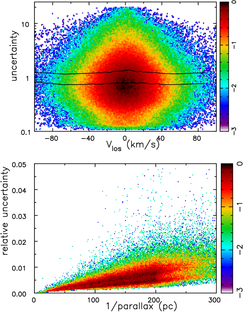
Figure 1: Top panel: The distribution of the line-of-sight velocity and its uncertainty for stars in our local sample. The two near horizontal lines mark the mean (upper) and median (lower) of the uncertainties in bins of ten thousand stars, indicating that the uncertainty is uncorrelated with this componet of velocity. Bottom panel: The distribution of stellar distances and their relative uncertainties in the selected sample. The distance is estimated directly from the Gaia parallax, and the uncertainty from their quoted value. In both panels, the logarithmic color scale shows the density of stars in the respective coordinates.

3 Action-angle variables

For simplicity, we consider motions of stars in the plane of the disc only and neglect the component of motion normal to the Galactic plane. Although some interesting features in the vertical motions have been found (e.g. Antoja et al., 2018; Bland-Hawthorn et al., 2018), most of the in-plane substructure is found for stars with small vertical action (Trick, Coronado & Rix, 2018). We therefore consider only stars whose vertical excursions are confined to $|z|<286\;$pc. Also, the rapid vertical oscillations of such stars should be largely decoupled from their horizontal motion (Sellwood, 2014). Thus we need consider just two actions, $J_{R}$ and $J_{\phi}\equiv L_{z}$ and two conjugate angles $w_{R}$ and $w_{\phi}$.

The classical integrals, $E=\Phi(R)+{1\over 2}(v_{R}^{2}+v_{\phi}^{2})$ and $L_{z}=Rv_{\phi}$, can readily be estimated from the Gaia data, together with some adopted model for the axisymmetric gravitational potential, $\Phi(R)$, in the disc mid-plane. We compute the radial action from the approximate expression

$$J_{R}={1\over\pi}\int_{R_{p}}^{R_{a}}\dot{R}dR\quad\hbox{with}\quad\dot{R}^{2}=2\left[E-\Phi(R)\right]-{L_{z}^{2}\over R^{2}},$$ (1)

where $R_{p}$ and $R_{a}$ are respectively the Galactic peri- and apo-centric distances of the star where its radial speed $\dot{R}=0$; the value is normalized by $\pi$ because the integral covers only half a full radial oscillation. This expression yields very nearly the same value (McMillan, 2011) for $J_{R}$ as obtained from the more-accurate “torus fitting” method that takes account of 3D motion. Physically, the radial action is an angular momentum-like variable that quantifies the magnitude of the radial motion of a star and, for disc stars, it is typically an order of magnitude smaller than the orbital angular momentum.

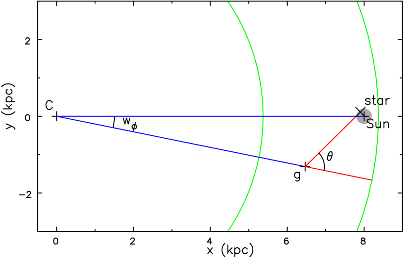
Figure 2: Sketch showing part of the Milky Way seen in projection; all the stars in our sample are confined to the lightly shaded region around the Sun. The Sun moves in clockwise direction about the Galactic centre, which is marked as C. A star in our sample might be located at the position shown by the X, and moves on a eccentric orbit between the radii marked with green circles at $R_{p}$ and $R_{a}$. The angle $w_{\phi}(>0)$ is the Galactic azimuth of the instantaneous position of the guiding centre, which is marked g, and is reckoned from the line from the Sun to C. The angle $w_{R}$, which is conjugate to the radial action, $J_{R}$, gives the phase of the star around its epicycle, but is not exactly equal to $\theta$, and is instead determined as described in the text. Note that $w_{R}>0$ for a star at the indicated position because stars move in a retrograde direction about their guiding centres.

Note that expression (1) for $J_{R}$, and the evaluation of the angle variables described below, require multiple orbit integrations for each star. Each individual quadrature is fast, so that the computational cost of evaluating them for all $312\,255$ stars in our sample is not particularly burdensome. However, the implicit relations between the angles and the peculiar velocities that we need to invert repeatedly require many millions more evaluations, making it computationally advantageous to choose the simple functional form, $\Phi(R)=V_{0}^{2}\log(R/R_{0})$ implying an exactly flat rotation curve, for the local radial variation of the Galactic gravitational potential. We have preferred this form over the Galaxy model proposed by Bovy (2015), even though Bovy’s coordinate conversions are effected quite efficiently using a local “Stäckel fudge” (Binney, 2012). We have verified that the distribution of values of the actions and angles is closely similar whichever of these two assumptions is adopted, and the features in the distributions of action-angle variables are insensitive to the chosen model.

Figure 2 illustrates the meaning of the angle $w_{\phi}$, which is the Galactic azimuth of the star’s guiding centre and we choose $w_{\phi}=0$ for the line from the Galactic centre that passes through the Sun. The angle $w_{R}$ is the phase of the star around its epicycle, and we choose $w_{R}=0$ at apocentre. These angles are computed from the positions reported by Gaia, but both increase with time at the uniform rates $\dot{w}_{R}=\Omega_{R}$ and $\dot{w}_{\phi}=\Omega_{\phi}\equiv L_{z}/R_{\rm g}^{2}$, where $R_{\rm g}$ is the Galactic radius of the star’s guiding centre. The period of the radial oscillation defines the uniform rate

$$\Omega_{R}={2\pi\over\tau_{R}}\qquad\hbox{where}\qquad\tau_{R}=2\int_{R_{p}}^{R_{a}}\dot{R}^{-1}dR.$$ (2)

Since $w_{R}$ increases uniformly with time, it does not correspond precisely to the angular position of the star around its epicycle, marked $\theta$ in the sketch, because the radial motion is generally not perfectly harmonic. To evaluate $w_{R}$ for a star at a general point, we must integrate its orbit to find the time $t$ required for it to reach its present radius from the moment it passed through apocentre. Then $w_{R}=\Omega_{R}t$. It is always true that $w_{R}=\pm\pi$ exactly at pericentre and, because epicycle motion is slower in the outer part, $|w_{R}|\ga\pi/2$ as the star crosses the circle at $R_{\rm g}$ in respectively the inward and outward directions.

This discussion is valid for orbits of arbitrary eccentricity, but the radial motion becomes more nearly harmonic as the orbit eccentricity decreases, and the angular frequencies tend to the familiar definitions introduced long ago by Lindblad (e.g. Binney & Tremaine, 2008):

$$\Omega_{\phi}\rightarrow\Omega_{c}\qquad\hbox{and}\qquad\Omega_{R}\rightarrow\kappa,$$ (3)

where $R\Omega_{c}^{2}=d\Phi/dR$ and $\kappa^{2}=4\Omega_{c}^{2}+Rd\Omega_{c}^{2}/dR$.

We show that the mapping from the observed 4D Galactic phase-space coordinates of a star at $(R,\phi,v_{R},v_{\phi})$ to $(J_{R},L_{z},w_{R},w_{\phi})$ is well-behaved, and (as was stressed by Trick, Coronado & Rix, 2018) any features present in the one projection must necessarily appear in any other, although in a distorted form. In this paper we also demonstrate that action-angle coordinates have the additional advantage that they clarify the connection between the substructure and its probable dynamical origin.

4 Features in phase space

Figure 3 presents the phase space density of our star sample in four different projections. The top panel reproduces the helio-centric velocity-space $(U,V)$ distribution (Gaia collaboration: Katz et al., 2018), which manifests multiple features that have become known as streams. The stars are projected into the space of the two actions, $(L_{z},J_{R})$, in the second panel, which was also presented by Trick, Coronado & Rix (2018), where both actions are normalized by the angular momentum of the LSR. The parabolic lower boundary to this distribution results from our selection of stars that are today passing within $200\;$pc of the Sun, since those stars with $L_{z}\neq L_{z,0}$ will pass close to the Sun only if their orbits are sufficiently eccentric, i.e. the greater the value $|L_{z}-L_{z,0}|$, the larger $J_{R}$ must be for the star to be in our sample. The distribution in $(w_{R},J_{R})$ space is illustrated in the third panel, while the bottom panel shows the distribution in $(w_{R},w_{\phi})$ space.

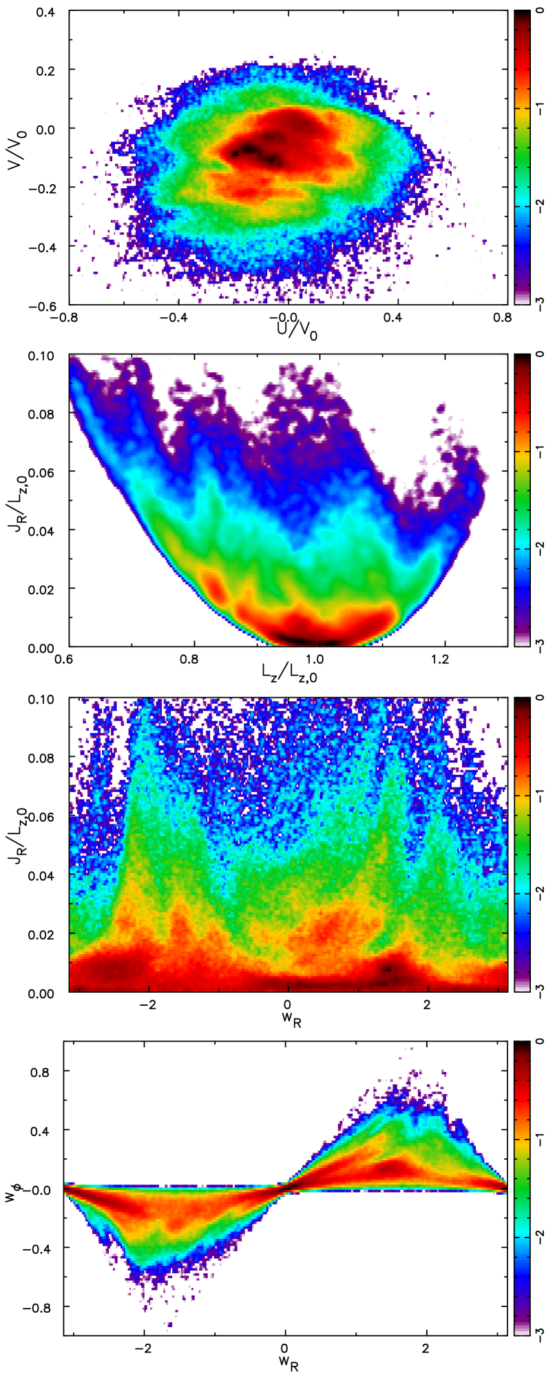
Figure 3: Four projections of the phase space density of our sample of nearby stars that stay close to the disk plane selected from GaiaDR2. The top panel shows the usual velocity-space $(U,V)$ distribution, the second panel the distribution in the space of the two actions $(L_{z},J_{R})$, the third panel the distribution in the space of the radial angle and action $(w_{R},J_{R})$, and the bottom panel the distribution in the space of the two angles $(w_{R},w_{\phi})$. The scales of $L_{z}$ and $J_{R}$ have been normalized by the angular momentum of the LSR. The color scale represents the logarithm of the relative density in each projection.

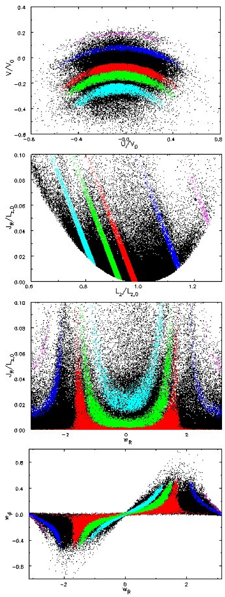
Figure 4: As in Fig 3, but showing the individual GaiaDR2 stars. The coloured stars were selected to highlight five separate sloping features in the second panel, and the other panels reveal where the same stars lie in the separate projections. We chose the centers of the sloping lines to intercept the $x$-axis at 0.85 (cyan), 0.925 (green), 0.98 (red), 1.16 (blue), and 1.33 (magenta).

Figure 4 illustrates how stars are mapped between these different coordinate projections. We have highlighted stars in five distinct groupings by colour, each coloured group being those stars lying within $\Delta L_{z}=0.01$ of a line of slope $-0.5$ in the second panel, for reasons that will become clear later. The intercept on the $L_{z}$ axis of each line was chosen by eye so that each selected group of stars included one of the more prominent features in that panel. The coloured points in the other panels of this Figure indicate where each group of selected stars lies in the three other projections. While the mappings from one panel to the other are complicated, they are well-behaved, and the highlighted stars lie in overdense regions in each projection.

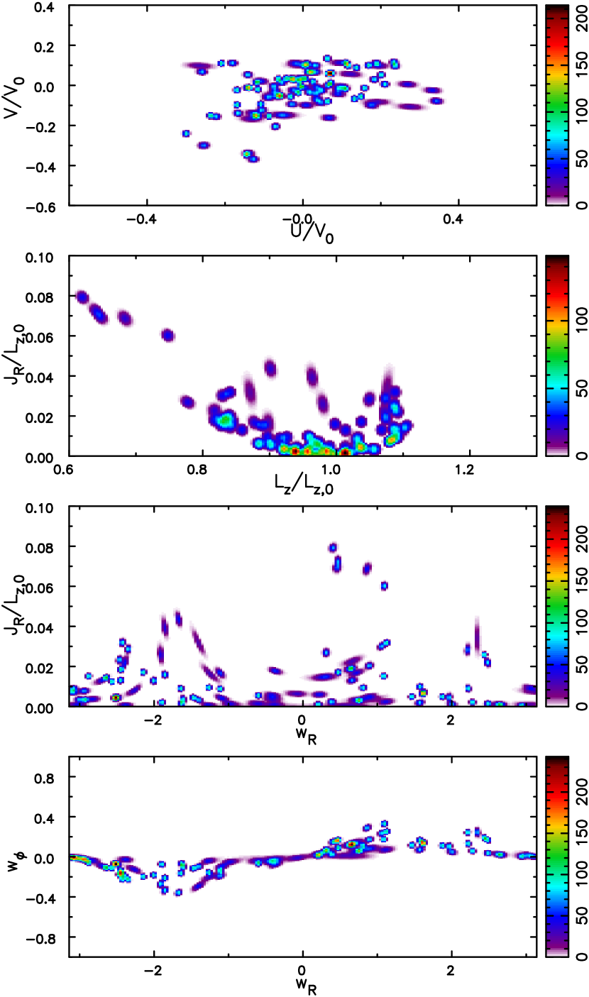
Figure 5: Estimated uncertainties in the quantities of interest here, derived for the first 100 stars in our sample. Each smudge shows the spread in values, coloured on a linear scale, that results from 1000 Monte Carlo realizations, using the uncertainties in each observed quantity, as reported for each star in GaiaDR2.

Figure 5 shows uncertainties in the derived quantities for the first 100 stars in our sample. For each star, we drew one thousand sets of new values for RA, dec, parallax, proper motions in RA and in dec, and radial velocity, each drawn from a Gaussian distribution with the observed value as the assumed mean and the Gaia estimate of the uncertainty in each quantity as the standard deviation. We used each realization of these adjusted coordinates to derive revised estimates of the velocities, actions and angles, and show the density of these new values in each projection. From this Figure, we see that the uncertainties in the derived quantities are generally small, but are somewhat larger for several stars, although the uncertainties, naturally, remain small compared with the widths of the features in Figure 3. The principal source of uncertainty appears to arise from the line-of-sight velocity, even though we discarded stars having uncertainties in this component $>5\;$km s^-1.

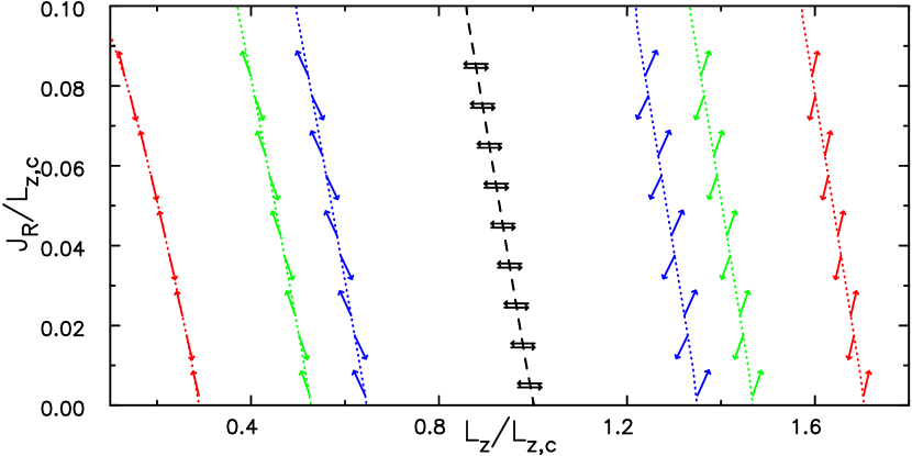
Figure 6: Scattering in action space for a self-similar $V=\;$const galaxy model. Both actions are normalized by $L_{z,c}$, which is the angular momentum of a circular orbit at corotation. The broken lines mark the separate loci of CR (black) and Lindblad resonances, colored red for $m=2$, green for $m=3$ and blue for $m=4$, computed using eq. (5) for orbits of finite eccentricity. The vectors, having arbitrarily chosen lengths, indicate possible changes computed from eq. (4). Formula (6) indicates that they should have slopes $l/m$.

4.1 Features in the action distribution

The substructure in the second panel of Figure 3 may be indicative of resonance scattering. Here we explain why we formed this view.

A test particle moving in a non-axisymmetric potential that rotates at the uniform rate $\Omega_{p}$ about the $z$-axis conserves neither its energy $E$ nor its angular momentum $L_{z}$, but Jacobi’s integral $E_{J}\equiv E-\Omega_{p}L_{z}$ is conserved (Binney & Tremaine, 2008). Hence, any changes to the energy and angular momentum of a star must be related as

$$\Delta E=\Omega_{p}\Delta L_{z}.$$ (4)

When the non-axisymmetric part of the potential is weak and has $m$-fold rotational symmetry, the motion of a star resonates with the rotating potential whenever

$$m(\Omega_{p}-\Omega_{\phi})=l\Omega_{R},$$ (5)

with $l=0$ for the corotation resonance (CR) and $l=\pm 1$ for the Lindblad resonances. At the ILR the star overtakes the wave, while at the OLR it is overtaken by the wave, and in both cases it experiences forcing at its natural radial frequency $\Omega_{R}$. Lynden-Bell & Kalnajs (1972) showed that only those stars that are in one of these resonances experience lasting changes to $E$ and $L_{z}$. The broken curves in Figure 6 mark the loci of the resonances in action space for $l=0,\;\pm 1$ and $m=2$ (red), $m=3$ (green), and $m=4$ (blue) perturbations in a simple $V=\;$constant galactic potential. These curves, which are calculated exactly for eccentric orbits using eq. (5), have similar negative slopes in any reasonable galaxy potential.

Sellwood & Binney (2002), in just a few lines of algebra, were able to show that scattering at any one of these resonances required not only that $\Delta E=\Omega_{p}\Delta L_{z}$, but that changes to the actions were simply related as

$$\Delta J_{R}={l\over m}\Delta L_{z}.$$ (6)

Formally, this relation is for near circular orbits, but the predicted slope holds for quite eccentric orbits, as illustrated by the vectors in Figure 6, with $\Delta J_{R}$ computed exactly from eq. (4) and not the approximation (6).

The horizontal vectors indicate that $\Delta J_{R}=0$ for moderate $\Delta L_{z}$ changes at CR where $l=0$, with the implication that radial migration at this resonance occurs without increasing random motion.

However, scattering at either Lindblad resonance should be along trajectories of almost constant slope $l/m$ in $L_{z}$-$J_{R}$ space, which therefore have positive slope at the OLR and negative at the ILR. Lynden-Bell & Kalnajs (1972) showed that stars may either gain or lose $L_{z}$ at all the major resonances, as indicated by the vectors in Figure 6, but they also showed that on average stars lose $L_{z}$ at the ILR and gain at the OLR, so formula (6) predicts net heating because the average $J_{R}$ is increased at both resonances. Notice that the scattering vectors for all initial $J_{R}$ values shift stars off the OLR as they gain or lose $L_{z}$, but the scattering vectors at the ILR are almost perfectly aligned with the resonance line for $m=2$ (red) and misalignment develops slowly as $m$ increases. This near coincidence is not just a pecularity of this potential and appears to hold in most other reasonable galactic potentials. Thus stars at the ILR remain close to the resonance as they are scattered, which allows large changes in $J_{R}$ to be built up, as we will demonstrate.

In summary, the second panel of Figure 3 manifests multiple density excesses having predominantly negative slopes that are similar to the slopes $\approx-0.5$ of all the major resonances in Figure 6. These features therefore suggest, but do not prove, that the stellar distribution in the neighbourhood of the Sun contains many stars that have been scattered at Lindblad resonances of several different disturbances having various pattern speeds.

It should now be clear why we chose to highlight stars along lines of slope $-0.5$ in Figure 4, since they could be stars that have been scattered at resonances. Whether the density excesses are or not created by resonant scattering, the highlighted stars in other panels show the loci of possible resonances in the other projections.

4.2 Features in the angle distribution

The third panel of Figure 3 shows the distribution of the Gaia stars as a function of $w_{R}$ and $J_{R}$. As for all other projections of the 4D distribution, we see a rich substructure. Our attempts to reproduce features in the different projections are described in §5, where the possible origin of the features in this projection will become clear.

The narrow distribution of $w_{\phi}$ values in the bottom panel, is a consequence of our selection of stars close to the Sun. We see that stars near apocentre ($w_{R}=0$) and pericentre ($w_{R}=\pm\pi$) all have $w_{\phi}\approx 0$, as expected. The largest values of $w_{\phi}$ arise for stars having eccentric orbits that are close to their guiding centre radii ($w_{R}\ga\pm\pi/2$), which is consistent with the sketch in Figure 2. Because the $w_{\phi}$ distribution is so dominated by selection effects, we have not found this last projection very informative.

By comparing the three other projections of the Gaia data with models in the next section, we will argue that the current stellar distribution has been sculpted by multiple resonances over time.

5 Predictions of various theories of spiral structure

Here we calculate how an originally smooth distribution of stars in an axisymmetric potential model is changed when perturbed by various time-dependent, non-axisymmetric perturbations. Our aim is not to create a single model that can match all the features in the Gaia data, but more modestly to show qualitatively how some of features might have arisen.

Each of our perturbations is motivated by one of the current theories for the origin of spirals in galaxies. Sellwood & Carlberg (2014) proposed that spirals result from transient modes, which we descibe more fully and test in §5.2. A number of authors have proposed that spirals are material arms, and we examine the consequences of this hypothesis in §5.3. Toomre & Kalnajs (1991) and D’Onghia et al. (2013) imagine that spirals result from the responses to mass clumps within the disk, which we model in §5.4. Finally, Bertin & Lin (1996) propose that spirals are long-lived, quasi-steady density waves, and we discuss their picture in §5.5.

5.1 Method

We employ the method pioneered by Dehnen (2000), which assumes some reasonable distribution function (DF) for the Galaxy before the perturbation was introduced and uses the fact that the DF is conserved along any orbit from the moment a perturbing potential is added to the present day. Bovy (2015) also implemented the technique in the python package galpy. Since we need to know the DF only where we wish to compare it with data, its current value at any point $(R,\phi,v_{R},v_{\phi})$ can be obtained by integrating an orbit from that point backwards in time over the history of the perturbation to when the adopted model was smooth and axisymmetric, where the value of the DF can be obtained from its coordinates $(R^{\prime},\phi^{\prime},v_{R}^{\prime},v_{\phi}^{\prime})$ at that earlier moment.

We adopt this method to model phase space at the location of the Sun. For each point in $(L_{z},J_{R})$ space, say, we must determine what the values of those variables imply for the instantaneous velocities of a star that also passes through the position of the Sun. That is we must find the $(R,\phi,v_{R},v_{\phi})$ coordinates of that orbit for fixed $R=R_{0}$ and $\phi=0$. Trivially, $v_{\phi}=L_{z}/R_{0}$, and we map $(L_{z},J_{R})\rightarrow(E,L_{z})$ and then use $v_{R}^{2}=2[E-\Phi(R_{0})]-(L_{z}/R_{0})^{2}$. We then integrate back in time to find where the orbit was before the perturbation, to find the value of the DF at the starting point in phase space. Note the two possible signs of $v_{R}$ imply that two separate locations $(R^{\prime},\phi^{\prime},v_{r}^{\prime},v_{\phi}^{\prime})$ before the perturbation was introduced map to the same point in $(L_{z},J_{R})$ space, and we therefore sum both DF values. The calculation when $w_{R}$ is pre-specified is more difficult, since we need a numerical search over $(E,L_{z})$ for the unique orbit that passes through $(R,\phi)=(R_{0},0)$ with phase $w_{R}$ and radial action $J_{R}$; once found, the $v_{\phi}$ and $v_{R}$ values are determined as before, but the value of $w_{R}$ removes the sign ambiguity of $v_{R}$.

We calculate the perturbed DF at the point $(R,\phi)=(R_{0},0)$, and make no attempt to average over the small area of radius 200 pc that contains the stars that we compare with our models. Our selection of such nearby stars was partly motivated by the need to be able to neglect gradients in phase space across this area.

We assume a ${\rm sech}^{2}\gamma t/2$ time dependence for every perturbation, which asymptotes to exponential growth as $\exp(-\gamma t)$ for $\gamma t\ll-1$ and begins to decay after peaking at $t=0$. Typically, the value of $\gamma=0.1\Omega_{p}$. We begin the integration at $t=1.36\;$Gyr, which is six orbit periods at the Sun ($2\pi R_{0}/V_{0}$) after the perturbation peaked at $t=0$, and integrate backwards in time to when the perturbation had negligible amplitude. The choice of six orbit periods after saturation allows the perturbation to decay somewhat, but is before some of the perturbed features become affected by a slow phase wrapping. We justify this on the grounds that continued evolution of a single perturbation would not be observable in the Gaia data because all theories, bar one, predict successive perturbations on a time-scale of a few orbits. The exception is the quasi-steady mode theory of Bertin & Lin (1996) that we argue (§5.5) predicts no phase space changes at all.

Our unperturbed Milky Way model is locally approximated as a disc having a simple Gaussian velocity distribution, with radial velocity dispersion $\sigma_{R}=0.13V_{0}$. The precise degree of random motion in the disc not very important, since we are here concerned with the qualitative relative changes produced by each perturbation, and do not attempt a quantitative comparison. The DF is

$$f(E,L_{z})\propto\exp(-1.5R_{g})e^{-{\cal E}/\sigma_{R}^{2}},$$ (7)

where $R_{g}=L_{z}/V_{0}$ is the guiding center radius and ${\cal E}=E-E_{c}(L_{z})$, is the excess energy above that of a circular orbit at $R_{g}$; $E_{c}=\Phi(R_{g})+V_{0}^{2}/2$. The $\exp(-1.5R_{g})$ factor was chosen to yield about the right variation with $L_{z}$. We “observe” the perturbed DF that results from each adopted perturbation from the location of the Sun at $R_{0}=8\;$kpc and $\phi=0$, and in the following figures we normalize the phase space density by its maximum value in every projection.

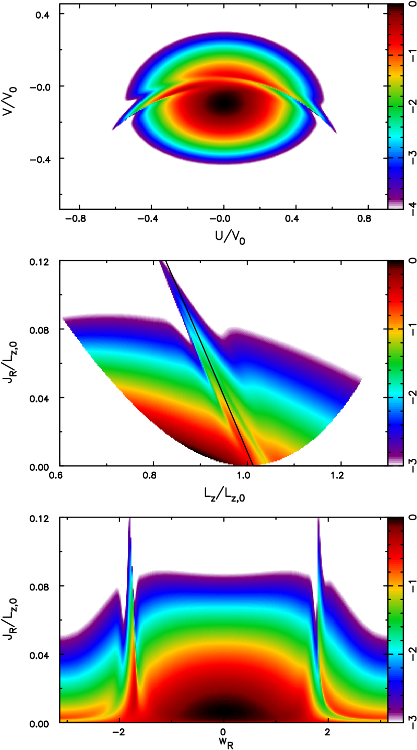
Figure 7: The predicted phase-space density of stars in three projections after our model spiral mode, described in the text, has grown and started to decay. The DF is largely undisturbed, except for features resulting from ILR scattering, that are broadened by the time dependence of the perturbing potential. The locus of the ILR is marked by the line in the middle panel. As above, the color scale represents the logarithm of the relative density in each projection.

5.2 A transient spiral mode

Sellwood & Carlberg (2014) proposed that spirals result from relatively short-lived unstable modes. Specifically, this description means that each perturbation is a standing wave oscillation, having a constant shape that rotates at a steady rate and grows exponentially until it saturates. Their simulations revealed that each coherent mode had a lifetime at moderate amplitude of some 10 rotation periods at its corotation radius, and the disk generally supported a few such modes simultaneously, with new instabilities developing in constant succession. The superposition of several coherent modes gave rise to the continuously changing patterns that are observed in most simulations. While the classical density wave theory (Bertin & Lin, 1996) also invokes modes, those authors expect each mode to be very slowly growing, or even “quasi-steady”, and the disk would support rather few such modes; i.e. they have a very different picture from that proposed by Sellwood & Carlberg (2014).

In order to calculate what to expect from a single transient spiral of the kind described by Sellwood & Carlberg (2014), we chose a 3-armed spiral perturbation with a pattern speed $\Omega_{p}=14.4\;$km s^-1 kpc^-1, for which the ILR lies at 8.1 kpc. We adopted a logarithmic spiral potential that had a pitch angle of $26^{\circ}$ and a radial variation that peaked at corotation and decreased as a quartic polynomial to zero at a radius that was 80% of that of the ILR – i.e. it was weak, but non-zero, a little interior to the ILR. As described above, it had a ${\rm sech}^{2}$ time dependence, with the asymptotic growth rate $\gamma=0.1\Omega_{p}$. We believe these choices to be reasonable. The scattering plots we present below were little changed when we employed a more tightly wrapped spiral, and differed only slightly for $m=2$ or $m=4$ patterns because of the slight slope changes to the scattering vectors in Figure 6. We have also experimented with wide variations in the pattern speed as we report below.

Although Sellwood & Carlberg (2014) identified growing modes, and showed that the frequency persisted for some time after saturation, the assumption we have made here that the shape remains the same as the disturbance decays is convenient, but probably too simple.

Figure 7 shows three projections of the phase space density of stars for this first case. The DF is largely undisturbed in all three panels except for narrow features that have been caused by ILR scattering, and each feature in these noise-free projections illustrates the bi-directional nature of the scattering expected from Figure 6. Both actions are normalized by the $L_{z}$ of the LSR in the middle panel, and the requirement that the stars must pass through the solar position naturally creates the parabolic lower boundary. The black line shows the locus of the ILR, with the scattering vectors (shown in green for this $m=3$ pattern in Figure 6) being responsible for its slight misalignment with the scattering tongue, which clearly shows the expected heating. Similar features are seen in the Gaia data (Figure 3) and have also been reported in simulations (Sellwood, 2012; Sellwood & Carlberg, 2014).

The bottom panel of Figure 7 shows $J_{R}$ as a function of its conjugate phase $w_{R}$, which reveals that the density in this space is also no longer smooth. Again we see that the DF is undisturbed over most of this projection of phase space. The variation at high $J_{R}$ is because stars of different $w_{R}$ that are now at the Sun have different home radii, where the DF has different normalizations. Also the sharp features near $|w_{R}|\simeq 2$ are for stars that were strongly scattered by the ILR and are now moving in their epicycles, both inward and outward, past the Sun.

In an earlier paper, Sellwood (2010) argued that all strongly scattered stars should have the same values of $mw_{\phi}+lw_{R}$. It is clear that this expectation was wrong, since we now see two sharp features near $|w_{R}|\simeq 2$. The fact that it is symmetrical about $w_{R}=0$ (apocentre) is not a coincidence, since recalculating with a shift of the intial phase of the spiral did not alter the symmetry about $w_{R}=0$ or the positions of the scattering features, and only minor details of the sharp features differed.

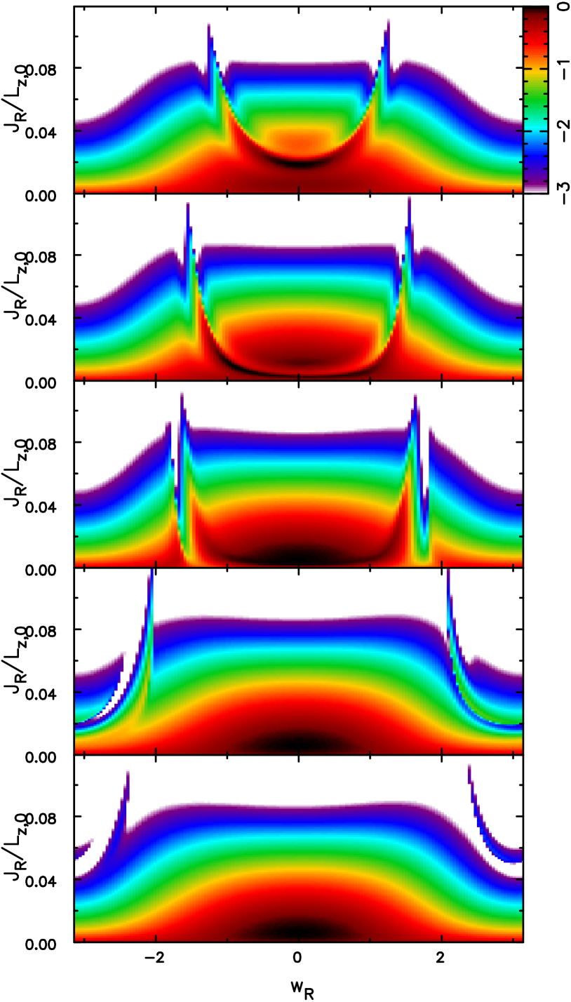
Figure 8: The effect on the $(w_{R},J_{R})$ distribution of changing the pattern speed of the spiral perturbation. From top to bottom, the adopted pattern speeds in km s^-1 kpc^-1 of our $m=3$ pertubation are 17.1, 15.7, 14.8, 12.5, and 10.9.

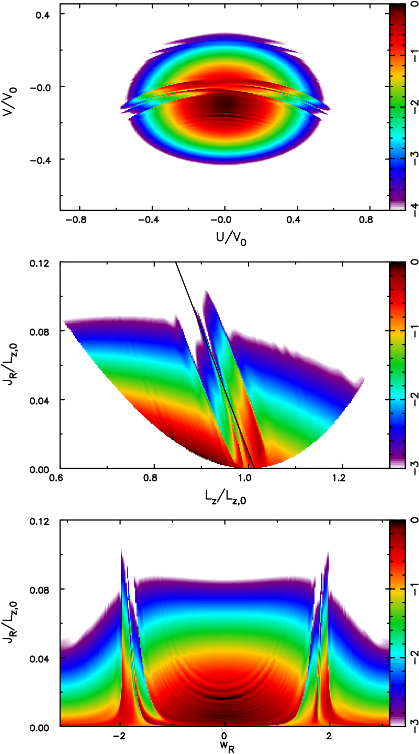
Figure 9: The predicted phase-space density of stars when the pattern speed of the spiral mode is raised so as to place the observer near the OLR. The locus of the OLR is marked by the line in the middle panel, where resonance scattering has created a broad feature in which stars have been shifted both up and to the right and down and to the left. Remarkably, the changes in the bottom panel resemble those in Figure 7. The color scale has the same meaning as in Figure 7

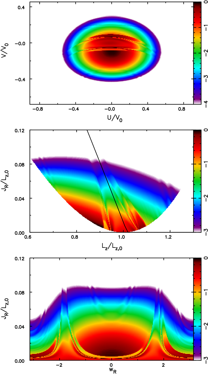
Figure 10: The predicted phase-space density of stars when the pattern speed of the spiral mode is adjusted so as to place the observer near CR. The locus of the CR is marked by the line in the middle panel. Changes to DF were remarkably mild, even though the perturbation amplitude was a maximum at this radius. The color scale has the same meaning as in Figure 7

Changes to the pattern speed of the spiral cause, as expected, a vertical shift to the scattering feature in the top panel of Figure 7 and a horizontal shift to the scattering tongue in the middle panel. The changes in the $(w_{R},J_{R})$ distribution are more interesting and are illustrated in Figure 8. In each case, the observer remains at the Sun’s position. The middle panel shows the effect of moving the ILR to a point just interior to the Sun, which caused the stars near apocentre $(w_{R}=0)$ to be affected and again those with enough radial action to have been strongly perturbed by the resonance produced similar peaks, also near $|w_{R}|=\pi/2$ but curving towards $w_{R}=0$ for lower values of $J_{R}$. Raising the pattern speed to higher values shifted the ILR farther inwards, giving rise to the features shown in the top two panels of Figure 8. As the ILR was shifted to larger radii (bottom two panels), the scattering features very gradually moved towards $w_{R}=\pm\pi$ (for stars at pericentre) and become weaker. Note that the farther the resonance from the solar radius in either direction, the less the DF is disturbed for small $J_{R}$ over all $w_{R}$. All this behaviour seems physically very reasonable.

The consequence of scattering at the OLR is shown in Figure 9, for which we adopted a pattern speed of $\Omega_{p}=40\;$km s^-1 kpc^-1. In this case, the observer is just interior to the resonance, so the features in the bottom panel curve towards $w_{R}=0$, since stars of low $J_{R}$ that have been affected by the resonance are near their apocentres, which is the opposite of the situation shown in Figure 7. More interesting is the feature in the middle panel; again the overall slope of the feature is negative, but at this resonance the scattering vectors have positive slope (Figure 6) with the consequence that scattering shifts higher phase space density both up and to the right and down and to the left. Furthermore, since stars are moved off resonance as they are scattered, we do not see the pronounced peak that was created at the ILR (Figure 7) and the spikes in bottom panel are less pronounced.

It is noteworthy that adjusting the pattern speed to $\Omega_{p}=27\;$km s^-1 kpc^-1, so that the CR was at $8.13~{}$ kpc, i.e. just exterior to the Sun left phase space near the Sun almost unchanged by the perturbation, as shown in Figure 10. This result is consistent with the prediction of formula (6), where stars simply change places with no heating. Furthermore, Lynden-Bell & Kalnajs (1972) showed that stars away from the major resonances suffer no lasting changes to their integrals, and we find similarly mild changes for observers located in a broad swath of radii around CR where few stars are found that have been affected by either of the Lindblad resonances.

5.3 A material arm model

A number of authors (e.g. Grand et al., 2012a, b; Baba et al., 2013; Roca-Fàbrega et al., 2013; Michikoshi & Kokubo, 2018) have argued that the spirals in their simulations are swing-amplified features having pitch angles that change continuously with time at a rate that is consistent with the local shear rate in their adopted galaxy model. In other words, the features are material arms, and not density waves. Hunt et al. (2018), using the galpy code (Bovy, 2015), adopted a potential of such a disturbance, combined with a model of the MW bar, to calculate its effect on the distribution of stars in $(U,V)$-space, and argued that some cases resembled the distribution of Gaia stars.

Although the disturbance they adopted indeed sheared, it did not seem to us to resemble the classic image of swing-amplification presented by Toomre (1981). We have therefore adopted the different potential perturbation that is illustrated in Figure 11. The radial variation has peak amplitude at some chosen $R_{c}=V_{0}/\Omega_{c}$ and is again as a quartic function that drops to zero at $R=R_{c}(1\pm 0.76)$. The azimuthal behaviour is that of a logarithmic spiral at all times, with the angle to the radius vector $\psi=\Omega_{c}(t-t_{0})$, which therefore changes as the perturbation shears with the flow; it is radial at $t=t_{0}$ and $\psi>0$ for a trailing spiral. Its overall amplitude also scales with time as ${\rm sech}^{2}\beta$ where $\beta=0.1[\Omega_{c}(t-t_{0})-m]$, and $m$ is the angular periodicity of the pattern; this shift in the argument ensures that the peak amplitude occurs at a trailing pitch angle of $45^{\circ}$, as expected for a flat rotation curve. The factor 0.1 gives about the right variation in amplitude around the peak and asymptotic growth and decay rates $\sim e^{-2\beta}$ for $|\beta|\gg 1$. We choose the maximum potential amplitude $=0.02$ at $R_{c}=9\;$kpc at a trailing angle of $\psi=45^{\circ}$.

Figure 11: Contours of the negative part of the perturbation potential, which varies sinusoidally with azimuth, adopted for the material spiral arm model in a clockwise rotating galaxy model. The model was motivated by the “dust-to-ashes” figure in Toomre (1981). The times in the upper right corner of each frame are in units of $R_{c}/V_{0}$, where $R_{c}=9\;$kpc is the radius of the potential maximum, which is marked by the dashed circle. See the text for further details.

Note this potential perturbation was chosen to mimic a swing-amplified spiral, but unlike that presented by Toomre (1981), it has no underlying dynamics. The potential function contains tightly-wrapped ripples for $\Omega_{c}|t-t_{0}|\gg$ a few, which in reality should be washed out by random motion in a warm disc. Also, the disturbance in our model has peak amplitude at $R_{c}$ at all times, which ignores the radial propagation of the wave packet at the group velocity, as occured in Toomre’s dynamically self-consistent calculation. However, both these effects occur only when the spiral is quite tightly wrapped, i.e. when our perturbed amplitude is weak. In summary, our model captures the material shear of the disturbance while the amplitude is large and the pattern open, which is the behaviour of the simulations as described in the above-cited papers, while omitting any dynamical details of the early and late evolution, when the amplitude is very low.

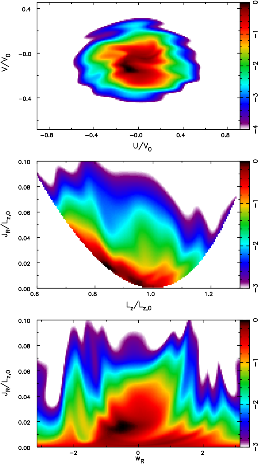
Figure 12: The distribution of stars in three different projections of phase space, observed from the Sun’s location, that results from applying the bi-symmetric material spiral arm perturbation described in the text. The top panel shows the distribution of velocities, the middle panel of actions, and the lower panel the angle $w_{R}$. The color scale has the same meaning as in Figure 7

Figure 12 presents three separate projections of the phase space distribution of stars that results from this disturbance. This quite strong perturbation has caused significant changes to the DF; naturally, scaling down the amplitude of the perturbation results in milder changes. Unlike for the spiral mode considered above, the individual features are quite broad and the entire distribution in every projection has been sculpted by the perturbation. We have experimented with shifting the radius of the density maximum to $R_{c}=7\;$kpc, i.e. interior to the Sun’s position, which again results in changes to the entire distribution in all three projections, but with the similarly broad peaks in differing locations.

We have also considered a 4-armed material spiral perturbations, which resulted in more regular “corrugations” in all three projections of the phase space density. The corrugations were present both when the potential maximum was interior or exterior to the Sun’s location.

5.4 A dressed mass clump

Toomre & Kalnajs (1991) developed the idea that co-orbiting mass clumps within the disc create a “kaleidoscope” of transient spiral features, which are caused by the collective response of the underlying disc to density inhomogeneities. The local simulations by these authors, in which shot noise from particles themselves created the inhomgeneities, were extended to global simulations by D’Onghia et al. (2013). The latter authors found that a sprinkling of heavy particles produced evolving multi-arm spiral patterns in their rather low mass disc. They also reported that non-linear effects could cause activity to persist after a single driving clump was removed.

It should be noted that each heavy particle quickly becomes dressed by an extensive trailing wake, whose mass far exceeds that of the imposed mass, and that the wake orbits at the angular rate of the perturbing source mass. The spiral patterns that result are caused by the superposition of these wakes, each of which has its own pattern speed.

In order to calculate changes in phase space density that would be predicted by a simplifed model of this type, we must use the perturbing potential of a dressed point mass. The response of a locally stable stellar disc to a point mass orbiting at the circular speed was originally calculated by Julian & Toomre (1966) in the well-known “sheared sheet” model that neglects curvature. The $(R,\phi)$ coordinates in the disc become

$$x=R-R_{c}\qquad\hbox{and}\qquad y=R_{c}\left[\phi-\Omega_{c}(t-t_{0})\right]$$ (8)

in the sheared sheet, where $\Omega_{c}$ is the circular angular frequency at $R_{c}$, the radius of the sheet centre, which is the location of the perturbing mass and therefore the corotation radius of the disturbance.

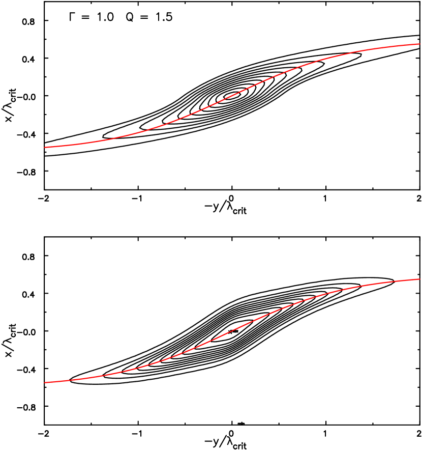
Figure 13: The upper panel contours the negative potential of the response density to a steady, coorbiting mass, computed by the method of Julian & Toomre (1966) in the sheared sheet, for a $V=$const disc with $Q=1.5$. The $(y,x)$ coordinates, defined in the text, are in units of $\lambda_{\rm crit}$. The lower panel shows the analytic approximation adopted here; the ridge-line of the approximate potential is marked in red and reproduced in the upper panel.

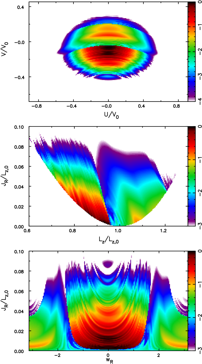
Figure 14: Three phase space projections resulting from a dressed mass clump model, whose centre orbits at $R=9\;$kpc, observed at $R=8\;$kpc, as usual. The color scale has the same meaning as in Figure 7

The top panel of Figure 13 presents contours of the perturbed potential computed using the mathematical apparatus devised by Julian & Toomre (1966). The spatial scale of the response density in the Figure can be converted to physical units by multiplying by $\lambda_{\rm crit}=4\pi G\Sigma/\kappa^{2}$, where $\Sigma$ is the disc surface density, and $\kappa$ the epicyclic frequency, both reckoned at $R=R_{c}$; in the self-similar Mestel disc $\lambda_{\rm crit}=2\pi Rf$ at any radius, where $f$ is the fraction of active mass. The Figure illustrates the potential of a wake for a $V=$const. disc with $Q=1.5$.

To use this perturbing potential in Dehnen’s method, we must convert $(R,\phi)$ to $(x,y)$ using equations (8) and scale them by an adopted value for $\lambda_{\rm crit}$. It is inconvenient to adopt this exact potential, because it is computed only over the rectangle shown; the perturbed potential on the boundaries is small, but non-zero, which would introduce mild discontinuities as stars crossed the boundaries that would be problematic when integrating orbits. We have therefore adopted the analytic approximation for the perturbing potential illustrated in the lower panel of Figure 13. Its functonal form is

$$\Phi_{w}(y,x) = -Ae^{-a}$$

$$a = y^{\prime 2}+x^{\prime 2}\left(1+100\sqrt{x^{\prime 2}+y^{\prime 2}}\right)$$ (9)

$$y^{\prime} = y/\lambda_{\rm crit}$$

$$x^{\prime} = x/\lambda_{\rm crit}-0.6\tanh(\pi y^{\prime}/4),$$

with $A$ being a scaling constant. The line $x=0.6\lambda_{\rm crit}\tanh(0.25\pi y/\lambda_{\rm crit})$, is the ridge line of the approximate potential, and is marked in red in both panels of the Figure. We consider this function to be an adequate approximation to the potential of a dressed particle.

It should be noted that the potentials shown in Figure 13 are that of the steady response to a constant perturbing mass. Julian & Toomre (1966) reported that the wake grows quickly after the introduction of a perturbing mass, and it takes only $\sim 5$ epicycle periods to asymptote to a steady response. Thus the wake of a growing mass would be only slightly weaker, unless the growth rate is very high.

We chose $\lambda_{\rm crit}=\pi R_{c}/2$, appropriate for a 1/4 mass Mestel disc for which half the circular speed arises from the disc attraction, and which very roughly corresponds to the situation over the massive part of the disc in the simulations by D’Onghia et al. (2013). We also adopt the same overall $\hbox{sech}^{2}$ time dependence as in our other models, set the radius of the co-orbiting mass clump to be at $R_{c}=9\;$kpc, and the potential perturbation scale $A=0.02$ so as to produce changes to the phase space density that are comparable in magnitude to those presented previously. The outcome is shown in Figure 14. This perturbation produces significant fine-scale substructure, especially for $L_{z}<L_{z,0}$, which also appears in the lower panel for $|w_{R}|\la\pi/2$. Shifting the perturber to $R_{c}=7\;$kpc, i.e. inside the solar radius, produced similar fine substructure except that, in this case, it appeared for $L_{z}>L_{z,0}$ and $|w_{R}|\ga\pi/2$.

The extensive fine-scale structure in this model differs from results obtained for the two previous perturbations: the spiral mode model (Figure 7) and the material arm model (Figure 12). In the present case, the wake has no rotational symmetry, and a relatively narrow azimuthal extent. A sectoral harmonic ($e^{im\phi}$) decomposition of such a disturbance would result in many $m$ components having significant amplitude, and $l=\pm 1$ resonances must arise for each separate $m$ component, which are ever closer to the radius of the source as $m$ rises. It seems possible that the large number of fine features could have been created by such resonances, but we defer detailed pursuit of this idea to a later paper.

5.5 Quasi-steady density waves

We do not present a calculation for the spiral density wave model of Bertin & Lin (1996). Although Sellwood (2011) demonstrated that their model had serious problems, this criticism was ignored by Shu (2016), who continued to argue for the quasi-steady mode theory in his review.

Their model attributes “grand design” spirals to slowly growing, bi-symmetric modes. Since their picture also suggests that the mode is “quasi-steady”, it should not have begun to decay, as we assumed for the transient mode model in §5.2. Predictions for a currently existing pattern could readily be calculated, indeed Dehnen (2000) devised his method to make predictions for the Milky Way bar. The most recent density-wave model for the Milky Way is that presented by Lin, Yuan & Shu (1969), which we could test. However, Shu (2016) argues that the situation in the Milky Way is now known to be more complex than the earlier paper assumed, with evidence for a 4-arm pattern, which he argues may possibly result from subharmonics or from superposed patterns, perhaps with one being a response to the bar.

In the absence of a specific, testable model from this group, we make a few general observations. Their picture of spiral wave generation invokes a $Q$-barrier to shield the mode from damping at the ILR, and therefore the principal cause of features in the phase space distribution in the transient spiral mode model would be absent in their picture. Also the CR has a neutral effect (Figure 10). Furthermore, since spirals in this model are long-lived and slowly evolving, these authors argue that most galaxies will have supported rather few such patterns. We would therefore expect that the extensive structure observed by Gaia in the local phase space distribution of stars in the Milky Way (Figure 3) would not be predicted by their quasi-steady spiral wave theory.

5.6 Discussion

The results presented for the three separate transient spiral arm models show that each gives rise to distinct predictions for the change in the density of stars in all three projections of phase space. Furthermore, all three scenarios expect that the Galaxy has supported many spiral episodes that have peaked at different radii, which in the case of the Sellwood & Carlberg (2014) mode theory would correspond to different pattern speeds.

For many reasons, we do not here attempt to make a quantitative comparison between the prediction of these models and the Gaia data presented in Figure 3. First, the data suggest that the features in phase space result from a succesion of perturbations, but we have so far computed the consequences of only single disturbances. Although scattering by a single spiral mode produces only symmetric features in the $(w_{R},J_{R})$ plane, as shown in the bottom panels of Figures 7–9, it may be possible that successive spiral disturbances could give rise to some of the asymmetries in the third panel of Figure 3. Second, it is likely that the local phase-space distribution of stars has also been scuplted by other perturbations, notably the bar in the Milky Way (Bland-Hawthorn & Gerhard, 2016) but also perhaps tidally induced responses, which would need to be included in any comprehensive model to confront the data. Third, we have made no attempt to match DF of the Milky Way, so that our choice of the undisturbed DF yields a good match of the pertubed data to the observations. Fourth, features in phase space may be blurred over time as stars are scattered by giant molecular clouds. Building a comprehensive model that includes all these aspects would be a major undertaking, which we defer to later work.

Both the material arm model, Figure 12, and the dressed clump model, Figure 14, predict multiple features from a single disturbance of large enough amplitude, and therefore multiple such disturbances would probably produce quite complex structure in all phase-space projections. However, the salient aspect of the data in the second panel of Figure 3 are a few features of negative slope, consistent with resonance scattering by a few patterns of low $m$.

The groups of stars from the Gaia data in Figure 4 that we highlighted in different colours were each selected to lie within $\Delta L_{z}=0.01$ of a line of slope $-0.5$ whose intercept on the $L_{z}$ axis was chosen by eye so that each selected group of stars included one of the more prominent features in the second panel of Figure 3. Because the loci of all the major resonances have approximately this slope, we are unable to say whether any selected feature corresponds to an ILR or an OLR, neither can we identify the rotational symmetry of the perturbation that caused it, and therefore we cannot estimate a pattern speed for any of these possible disturbances.

The coloured stars in Figure 4 do not correspond to every feature in the distribution of Gaia stars, neither should they. The different scattering events, if that is what are highlighted, will have occurred successively, the Milky Way hosts a bar (Bland-Hawthorn & Gerhard, 2016), and the disc has possibly been subject to other perturbations that may have produced additional features in these different projections. However, the distributions of the variously coloured stars in Figure 4 are quite similar to the features in Figure 7, and the resemblance seems closer than to those predicted by either of the other models. Indeed, we chose the pattern speeds in Figure 8 to be such that the ILR of an $m=3$ spiral mode would correspond to each of the highlighted features in Figure 4. Note that these calculations were made for each pattern speed separately, whereas the Gaia data would reflect successive patterns that may account for some of the asymmetries in the $(w_{R},J_{R})$-plane. It should also be cautioned that this superficially compelling comparison, particularly in the $(w_{R},J_{R})$-plane, owes a lot to the fact that the appearance in each projection is determined by the mapping of the 4D distribution to each 2D surface, and the only really significant features are the resonant ridges in the middle panel.

We conclude that the data offer little support for the dressed mass clump model, none at all for the quasi-steady density wave model and, while the material arm model may not be excluded, the sharper features in the Gaia data appear more consistent with the transient spiral mode model of Sellwood & Carlberg (2014).

5.7 Material arms vs. modes

The popular claim (Grand et al., 2012a, b; Baba et al., 2013; Roca-Fàbrega et al., 2013; Michikoshi & Kokubo, 2018) that spiral arms are material features that shear with the flow reflects the apparent behaviour in the simulations. Sellwood & Carlberg (1984) at first presented evidence that their spirals were shearing, swing-amplified features, in agreement with these recent reports. But a few years later (e.g. Sellwood, 1989) they showed that the density variations in the same simulations could be decomposed into a number of underlying coherent, steadily-rotating waves.

In order to understand how the two interpretations can give rise to the same behaviour, the reader may find it helpful to watch the animation at http://www.physics.rutgers.edu/$\sim$sellwood/spirals.html, which shows that an apparently shearing, swing-amplified spiral can result from the super-position of two rigidly rotating patterns. Note also that the “dust-to-ashes” figure presented in Toomre (1981) was calculated as the superposition of multiple steady responses to a set of perturbers having a range of pattern speeds (private communication, A. Toomre c1986).

Thus the superposition of multiple steadily-rotating patterns of differing rotational symmetries, whose amplitudes vary on the time-scale of a few orbits, can readily be imagined as giving rise to the untidy and apparently random shearing spirals that are visible in all simulations. Indeed, Sellwood & Carlberg (2014) explicitly reported their own large-$N$ simulations of a low-mass disc that appeared to manifest the kind of material arms observed in simulations by other groups and showed from spectral analysis (their Fig 9) that the shearing features resulted from the superposition of multiple coherent waves.

While the swing-amplified interpretation of simulated spirals is very beguiling, and consistent with Toomre’s picture, it begs the question of what is the origin of the leading signal that is swing-amplified? None of the above-cited papers that have argued for this interpretation has even addressed this question, let alone provided a satisfactory answer.

If the patterns were linear responses to shot noise, even of dressed particles (Toomre & Kalnajs, 1991), their amplitude clearly should decrease as $N^{-1/2}$. This possibility was already disproved by Sellwood & Carlberg (2014) who compared the behaviour from simulations in which the particle number ranged over three orders of magnitude.

Other tests by Sellwood & Carlberg (2014) also ruled out that non-linear coupling was needed to produce large-amplitude spirals. After erasing any coherent mass clumps by azimuthal shuffling of the particles in a partly evolved simulation, they showed that the same coherent waves were present in parallel simulations both after shuffling and in the continued simulation without shuffling. Had density variations at the time of reshuffling been responsible for subsequent patterns, then shuffling would have been equivalent to a fresh start, and the amplitude of spirals would have grown as slowly, or more slowly because random motion had increased slightly. Instead they observed more rapid and coherent growth than in the first start. This result proved that the axisymmetric changes caused by the earlier evolution had created conditions for a vigorous, global, linear instability that was not present in the original smooth disc.

The prominent self-excited spirals that develop in every large-$N$ simulation of disc galaxy models, that exclude forcing by clumps, bars, or companions, require that they are true instabilities of the dynamical system that is represented by the particles. The swing-amplified material arm interpretation, while superfically attractive and a correct description of the apparent behavior, is simply not a viable theory for spiral arm formation. The interpretation that the apparent features result from superposition of a number of transient spiral modes was placed on a sound footing by Sellwood & Carlberg (2014) who also offered a mechanism that could produce exponentially growing, global modes in a dynamically modified disc. Our present finding that the distribution of local stars in action-angle space is more consistent with multiple spiral modes than with transient material disturbances provides further evidence in support of their picture.

It might be objected that the transient disturbance adopted in §5.3 was not dynamically self-consistent, and therefore not a fair test. However, a fair test would be to consider, as did Toomre (1981), a spiral that is the superposition of a number of steady waves, which we have already shown would be more consistent with the Gaia data.

6 Conclusions

The second data release from the Gaia mission has refined our view of the phase-space distribution of stars near the Sun. The components of their motion parallel to the Galactic plane have long been known to manifest detailed substructure, which was seen more sharply in the first view of the new data (Gaia collaboration: Katz et al., 2018). Adopting a simple axisymmetric model for the Milky Way that has a locally flat rotation curve, enabled us to compute action-angle variables for a sub-sample of likely thin-disk stars within a cylinder of radius 200 pc centered on the Sun, and Figure 3 shows the density of stars in four different projections of this 4D phase space. The well-known substructure in velocity space maps into rich substructure in these other variables, which we note has some of the characteristic features of Lindblad resonance scattering by multiple perturbations having a range of pattern speeds and low-order rotational symmetry.

In order to determine whether some of these features might have been caused by past spiral activity in the disc of the Milky Way, we computed the changes to the distribution of stars in phase space that would be caused by a single spiral pattern of the kind favored by each of the following three current theories for spiral arm formation: the transient spiral mode model (Sellwood & Carlberg, 2014), the swing-amplified model of material arms (e.g. Grand et al., 2012a, b; Baba et al., 2013; Roca-Fàbrega et al., 2013; Michikoshi & Kokubo, 2018), and the dresed mass clump model (Toomre & Kalnajs, 1991; D’Onghia et al., 2013). We also argued that the quasi-steady density wave model (Bertin & Lin, 1996) should not create pronounced features in the phase-space distribution of stars near the Sun. For each of the first three cases, we adopted a simplified transient potential that approximates that of an idealized, isolated spiral. We found that the inner Lindblad resonances of a single pure transient spiral mode produced the narrow features in phase space shown in Figure 7. Multiple broad features, see Figure 12, were created by a single shearing spiral, or material arm, and multiple fine features, Figure 14, resulted from the wake of single dressed particle. For each model, we experimented with changes to the pattern speed or, in the case of material arms, the radius of the perturbed potential minimum, and found that the locations of the features in each projection varied in ways that made dynamical sense.

We argued that the Gaia data are inconsistent with the dressed particle model, and while they could be consistent with the material arm model, some of the narrower scattering features in Figure 3 more strongly resemble the prediction of spiral modes that are expected to have had a variety of pattern speeds and rotational symmetries. Other considerations discussed in §5.7 strongly disfavour the swing-amplified material arm model, although we also explain that the superposition of a number of steady spiral modes can give the visual impression swing-amplified shearing evolution.

We do not here claim to have presented a model that can account for all the features in the 4D phase space distribution. The rich substructure in the distribution of Gaia stars deserves additional effort to fully understand its origin.

References

- Antoja et al. (2018) Antoja, T., Helmi, A., Romero-Gomez, M., et al. 2018, arXiv:1804.10196
- Antoja et al. (2009) Antoja, T., Valenzuela, O., Pichardo, B., et al. 2009, ApJ, 700, L78
- Baba et al. (2013) Baba, J., Saitoh, T. R. & Wada, K. 2013, ApJ, 763, 46
- Bensby et al. (2007) Bensby, T., Oey, M. S., Feltzing, S. & Gustafsson, B. 2007, ApJ, 655, L89
- Bertin & Lin (1996) Bertin, G. & Lin, C. C. 1996, Spiral Structure in Galaxies (Cambridge, MA: The MIT Press)
- Binney (2012) Binney, J. 2012, MNRAS, 426, 1324
- Binney & Tremaine (2008) Binney J. & Tremaine S. 2008, Galactic Dynamics (Princeton University Press, Princeton NJ) (BT08)
- Bland-Hawthorn & Gerhard (2016) Bland-Hawthorn, J. & Gerhard, O. 2016, ARA&A, 54, 529
- Bland-Hawthorn et al. (2018) Bland-Hawthorn, J., Sharma, S., Tepper-Garcia, T., et al. 2018, arXiv:1809.02658
- Bovy (2015) Bovy, J. 2015, ApJS, 216, 29
- Bovy et al. (2012) Bovy, J., Allende Prieto, C., Beers, T. C., et al. 2012. ApJ, 759, 131
- Bovy & Hogg (2010) Bovy, J. & Hogg, D. W. 2010, ApJ, 717, 617
- Chakrabarty (2007) Chakrabarty, D. 2007, A&A, 467, 145
- Dehnen (2000) Dehnen, W. 2000, AJ, 119, 800
- De Simone et al. (2004) De Simone, R. S., Wu, X. & Tremaine, S. 2004, MNRAS, 350, 627
- D’Onghia et al. (2013) D’Onghia, E., Vogelsberger, M. & Hernquist, L. 2013, ApJ, 766, 34
- Famaey et al. (2007) Famaey, B., Pont, F., Luri, X., Udry, S., Mayor, M. & Jorrissen, A. 2007, A&A, 461, 957
- Flynn et al. (2006) Flynn, C., Holmberg, J., Portinari, L., Fuchs, B. & Jahreiß, H. 2006, MNRAS, 372, 1149
- Gaia collaboration: Brown et al. (2018) Gaia collaboration: Brown, A. G. A., Vallenary, A., Prusti, T., et al. 2018, A&A, 616A, 1
- Gaia collaboration: Katz et al. (2018) Gaia collaboration: Katz, D., Antoja, T., Romero-Gó, M., et al. 2018, A&A, 616A, 11
- Grand et al. (2012a) Grand, R. J. J., Kawata, D. & Cropper, M. 2012a, MNRAS, 421, 1529
- Grand et al. (2012b) Grand, R. J. J., Kawata, D. & Cropper, M. 2012b, MNRAS, 426, 167
- Grand et al. (2015) Grand, R. J. J., Bovy, J., Kawata, D., et al. 2015, MNRAS, 453, 1867
- Hunt et al. (2018) Hunt, J. A. S., Hong, J., Bovy, J., Kawata, D. & Grand, R. J. J. 2018, eprint arXiv:1806.02832
- Julian & Toomre (1966) Julian, W. H. & Toomre, A. 1966, ApJ, 146, 810
- Jurić et al. (2008) Jurić, M., Ivezić, Z̆., Brooks, A., et al. 2008, ApJ, 673, 864
- Lin, Yuan & Shu (1969) Lin, C. C., Yuan, C. & Shu, F. H. 1969, ApJ, 155, 721
- Lynden-Bell & Kalnajs (1972) Lynden-Bell, D. & Kalnajs, A. J. 1972, MNRAS, 157, 1
- McMillan (2011) McMillan, P. J. 2011, MNRAS, 418, 1565
- Michikoshi & Kokubo (2018) Michikoshi, S. & Kokubo, E. 2018, arXiv:1808.08060
- Pompéia et al. (2011) Pompéia, L., Masseron, T., Famaey, B., et al. 2011, MNRAS, 415, 1138
- Quillen (2003) Quillen, A. C. 2003, AJ, 125, 785
- Quillen & Minchev (2005) Quillen, A. C. & Minchev, I. 2005, AJ, 130, 576
- Quillen et al. (2018) Quillen, A. C., De Silva, G., Sharma, S., et al. 2018, MNRAS, 478, 228
- Roca-Fàbrega et al. (2013) Roca-Fàbrega, S., Valenzuela, O., Figueras, F., et al. 2013, MNRAS, 432, 2878
- Schönrich et al. (2010) Schönrich, R., Binney, J. & Dehnen, W. 2010, MNRAS, 403, 1829
- Sellwood (1989) Sellwood, J. A. 1989, in Dynamics of Astrophysical Discs, ed. J. A. Sellwood (Cambridge: Cambridge University Press) p. 155
- Sellwood (2010) Sellwood, J. A. 2010, MNRAS, 409, 145
- Sellwood (2011) Sellwood, J. A. 2011, MNRAS, 410, 1637
- Sellwood (2012) Sellwood, J. A. 2012, ApJ, 751, 44
- Sellwood (2014) Sellwood, J. A. 2014, Rev. Mod. Phys., 86, 1
- Sellwood & Binney (2002) Sellwood, J. A. & Binney, J. J. 2002, MNRAS, 336, 785
- Sellwood & Carlberg (1984) Sellwood, J. A. & Carlberg, R. G. 1984, ApJ, 282, 61