Local Density of States induced near Impurities in Mott Insulators

Abstract

The local density of states near dopants or impurities has recently been probed by scanning tunneling microscopy in both the parent and very lightly doped compounds of the high-$T_{c}$ cuprate superconductors. Our calculations based on a slave-rotor description account for all the following key features of the observed local density of states: i) positions and amplitudes of the in-gap spectral weights of a single impurity; ii) the spectral weight transfer from the upper Hubbard band to the lower Hubbard band; iii) the difference between the cases of single and multiple impurities. For multiple impurities, our study explains the complete suppression of spectral weight observed at precisely the Fermi energy and links this property to zeros of the underlying bulk Green’s function of the Mott insulating phase.

Introduction.   The high-$T_{c}$ cuprate superconductors are generally interpreted as doped Mott insulatorsLee and Wen (2006). The undoped parent compounds are ordered antiferromagnetically. Although the parent compounds are three-band, charge transfer insulatorsZaanen et al. (1985), it is believed that the single-band Hubbard model (HM) provides an adequate effective description. The strong, onsite Coulomb repulsion, Hubbard-$U$, forbids two electrons to occupy the same Cu site, thereby creating a Mott gap $\propto U$ and splitting the electronic spectrum into the upper Hubbard band (UHB) and lower Hubbard band (LHB). Superconductivity arises from carrier-doping the parent compounds beyond a threshold concentration.

The rich properties of the doped cuprate Mott insulators suggest the importance of studying Mott insulators under dilute dopants or impurities. The local density of states (LDOS) near dopants/impuries in the parent Mott insulator has been studied through scanning tunneling microscope (STM) measurementsYe et al. (2013); Cai et al. (2015). These experiments have uncovered a number of features on the electronic excitation spectrum of a Mott insulator. For a single impurity, the in-gap states emerge from the UHB above the Fermi energy. When impurity concentration increases, the in-gap states gradually fill up the Mott gap, but a “V”-shaped dip forms near the Fermi energy. The observed dip means that the impurities or dopants cannot produce in-gap states exactly at the Fermi energy.

The experimental development is exciting as it bridges between the clean parent compounds and the heavily debated, lightly doped but metallic pseudogap regimesKeimer2015 . A systematic study of the Mott insulator in the presence of a single defect dopant or impurity is highly desirable. Previous efforts on this type of problemsLiu1992 ; Poilblanc1994 ; Leong et al. (2014) have been mostly numerical, which are restricted by finite-size effect, and have yet to achieve the understanding of the key experimental observations mentioned earlier.

In this Letter, we study the LDOS of single and multiple impurities in a Mott insulator based on a slave rotor representation of the HM in the thermodynamic limit. We find clear, impurity-induced in-gap bound states, descending from UHB as observed in Ref. Ye et al. (2013). In addition, we obtain the correct spectral weight transfer from the UHB to the LHB. Systematic calculations of the bound state energies and their corresponding spectral weights provide qualitative understandings about the experiments of Ref.Cai et al. (2015): i) the bound states cannot reach the Fermi energy; ii) the bound states with energies closer to the Fermi energy have smaller spectral weights. We show that the vanishing of the LDOS at the Fermi energy reflects the zeros of the Green’s function, i.e the Luttinger surfaceDzyaloshinskii2003 , of the underlying Mott insulator. That is a feature of considerable interest to the Mott insulator per se and to the physics of the pseudogap regime of the underdoped cuprates Konik2006 ; KYYang2006 ; Dave2013 .

The slave-rotor approach.   We consider the Hubbard model on a square lattice

$$H_{HM}(d)=\sum_{i}H_{at}(i)-\sum_{ij,\alpha}(t_{ij}d^{\dagger}_{i\alpha}d_{j\alpha}+h.c.),$$ (1)

in which $H_{at}(i)=\frac{U}{2}\Big{(}\sum_{\alpha}d^{\dagger}_{i\alpha}d_{i\alpha}-N/2\Big{)}^{2},$ $\alpha$ is the spin/orbital index and runs from $\alpha=1,\dots,N$, with N=2 for the one-band model. For simplicity, we consider only hopping between nearest-neighbor ($nn$) sites, $\langle ij\rangle$. The full energy spectrum of $H_{at}(i)$ can be economically represented by a rotor kinetic energy $H_{at}(i)\rightarrow U\hat{L}_{i}^{2}/2$ Florens and Georges (2002, 2004) with $\hat{L}_{i}=-i\partial_{\theta_{i}}$, which provides a tractable reference point for perturbative expansion in $t/U$. In this slave-rotor representation, the bare electron operator is written as product of the auxiliary rotor fields and a fermionic spinon operator $d_{i\alpha}\equiv f_{i\alpha}e^{-i\theta_{i}}$, with the constraint

$$\hat{L_{i}}=\sum_{\alpha}(f^{\dagger}_{i\alpha}f_{i\alpha}-1/2).$$ (2)

In place of the phase field one could work with the complex field $e^{i\theta_{i}}=X_{i}$, with the additional constraint $\lvert X_{i}\rvert^{2}=1$. The two constraints are enforced by introducing two Lagrangian multipliers, $h_{i}$ and $\lambda_{i}$. A saddle point solutionFlorens and Georges (2004); Lee and Lee (2005) (see Supplemental Materials, Eq. (S-1) for details) is found by decoupling the spinon-boson coupling term via

$$Q_{f,ij}=\mbox{$\langle X_{j}^{*}X_{i}\rangle$},\qquad Q_{X,ij}=\mbox{$\langle\sum_{\alpha}f_{j\alpha}^{\dagger}f_{i\alpha}\rangle$}.$$ (3)

From here on, we drop the subscript index ${ij}$ for $t$ and $Q_{f(X)}$. The spinon and $X$-field Green’s functions at the saddle-point level read

$$\begin{cases}G_{f,0}(\omega;\bm{k})=(\omega+h-Q_{f}\epsilon_{\bm{k}})^{-1},\\ G_{X,0}(\nu;\bm{k})=(-\nu^{2}/U+2ih\nu/U+\lambda+Q_{X}\epsilon_{\bm{k}})^{-1},\end{cases}$$ (4)

where $\epsilon_{\bm{k}}=-2t(\cos k_{x}+\cos k_{y})$ is the bare lattice dispersion function.

The electronic Green’s function is calculated via the rotor and spinon Green’s function according to

$$iG_{d}(t;\bm{x},\bm{x}^{\prime})=-G_{f}(t;\bm{x},\bm{x}^{\prime})G_{X}(-t;\bm{x},\bm{x}^{\prime}).$$ (5)

We are interested in the LDOS $\rho_{d}(\omega;\bm{x})=-(\pi)^{-1}\Im m[G_{d}(\omega;\bm{x},\bm{x})]$, expressed as

$$\rho_{d}(\omega;\bm{x})=\int d\omega^{\prime}\rho_{f}(\omega^{\prime};\bm{x})\rho_{X}(\omega-\omega^{\prime};\bm{x}),$$ (6)

where $\rho_{f}[\omega;\bm{x}]=-(\pi)^{-1}\Im m[G_{f}(\omega)]\,,{and}\,\rho_{X}[\omega]=-(\pi)^{-1}\Im m[G_{X}(\omega)]$.

The bulk Mott insulating phase is described at the saddle point level. Here, $Q_{X}=\mbox{$\langle\sum_{\sigma}f_{i\sigma}^{\dagger}f_{j\sigma}\rangle$}$ is a constant independent of the effective spinon hopping $Q_{f}$, and, thus, self-consistency is trivially satisfied. In this work we are interested in the large-$U$ limit, so we use $\lambda\simeq U/4$ throughout. At the saddle point, $\Im m[G_{f}(\omega^{\prime})]$ centers at $\omega^{\prime}=0$ with a bandwidth $W_{f}=4DQ_{f}$, which is small because $Q_{f}\ll U$; any impurity effects on $\Im m[G_{f}(\omega^{\prime})]$ per se would be on the same scale. In the convolution, $\Im m[G_{f}(\omega^{\prime})]$ can be regarded as a broadened $\delta$-function since $Q_{f}\ll U$. The Mott gap is primarily determined by $\Im m[G_{X}(\nu)]$, Therefore, the impurity-induced features of the electronic LDOS are mainly determined by the rotor fields, which shall be our focus in the following.

The induced rotor impurity potential.   We consider the case of a single impurity as experimentally studied in Ref.Ye et al. (2013), which is either a missing chlorine($Cl^{-}$) ion or a calcium($Ca^{2+}$) defect. The vacancy is charged, and creates an impurity potential. We mode it by a localized, onsite potential $V(\bm{x}_{i})$, where $\bm{x}_{i}$ denotes the vacancy position.

Consider a single on-site impurity at $\bm{x}_{0}$:

$$H_{1}=V\sum_{\sigma}d^{\dagger}_{\bm{x}_{0},\sigma}d_{\bm{x}_{0},\sigma}=V\sum_{\sigma}f^{\dagger}_{\bm{x}_{0},\sigma}f_{\bm{x}_{0},\sigma}.$$ (7)

While it corresponds to an impurity term for the spinons, the rotors and the spinons are subject to the constraint Eq. (2). Through the constraint, we expect the rotors to be perturbed by the impurity potential as well.

In the large-$U$ case we consider, it suffices to solve the constraint in the atomic limit. In the $X$-field representation,

$$\hat{L}_{i}=(h-X_{i}^{*}\partial_{t}X_{i})/U.$$ (8)

For the bulk state, we have $\mbox{$\langle\hat{L}\rangle$}=0\rightarrow h=0$. For arbitrary $h$, we have

$$\begin{split}&\mbox{$\langle\hat{L}\rangle$}=h/U-\frac{1}{2}\frac{h}{\sqrt{-h^{2}+\lambda U}}.\end{split}$$ (9)

Therefore, although a local impurity potential only explicitly couples to the spinons, the variation of the local spinon density $\delta n_{f}(\bm{x}_{0})=\delta\mbox{$\langle\sum_{\sigma}f^{\dagger}_{\bm{x}_{0}\sigma}f_{\bm{x}_{0}\sigma}\rangle$}$ induces variation of the Lagrangian multiplier $h$ through the constraint, which we shall label as $\delta h(\bm{x}_{0})$. Using the atomic limit result, $\delta h(\bm{x}_{0})$ is obtained by solving the following equation:

$$\frac{\delta h(\bm{x}_{0})}{U}-\frac{\delta h(\bm{x}_{0})}{2\sqrt{-\delta h(\bm{x}_{0})^{2}+\lambda U}}=\delta\mbox{$\langle n_{f}(\bm{x}_{0})\rangle$}.$$ (10)

Taking $\lambda=U/4$, we plot the solution of $\delta h(\bm{x}_{0})$ as a function of $\delta\mbox{$\langle n_{f}(\bm{x}_{0})\rangle$}$ in Fig. (1). To solve for the impurity states, we take $\delta\mbox{$\langle n_{f}(\bm{x}_{0})\rangle$}=\pm 1$, since $V$ of relevance to the experiments is on the order of $eV$, i.e. much larger than the spinons’ bandwidth. This solution gives us the upper bound of $h(\bm{x}_{0})$. For the rest of this work, we shall use $\delta h(\bm{x}_{0})\simeq 0.473U$ unless specified otherwise. Even though negative solution of $\delta h(\bm{x}_{0})$ is allowed here, they do not induce in-gap bound states, and thus shall be ignored. Then the impurity potential due to $\delta h(\bm{x}_{0})$ is

$$\begin{split}&\hat{H}_{X,\bm{x}_{0}}=ih_{0}(X^{*}_{\bm{x}_{0}}\partial_{t}X_{\bm{x}_{0}}-X_{\bm{x}_{0}}\partial_{t}X_{\bm{x}_{0}}^{*})\end{split}$$ (11)

where we label $h_{0}=2\delta h(\bm{x}_{0})/U$.

Impurity state Green’s function.

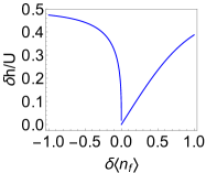
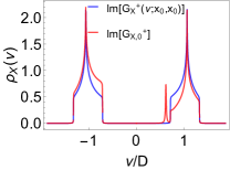
Figure 1: (Color online) (1) the solution of $\delta h(x_{0})$ plotted as a function of $\delta\mbox{$\langle n_{f}(x_{0})\rangle$}$; (1) the bulk rotor spectral function $\Im m[G_{X,0}^{+}(\omega;\bm{x},\bm{x})]$ (blue) compared with that on a single impurity, $\Im m[G_{X}^{+}(\omega;\bm{x}_{0},\bm{x}_{0})]$ (red) .

We now turn to calculating the LDOS of a single impurity in a Mott insulator using the $T$-matrix formalism. The full rotor Green’s function, to the first order in $h_{0}$ can be expressed as

$$\begin{split}&G_{X}(\nu;\bm{x}_{1},\bm{x}_{2})=G_{X,0}(\nu;\bm{x}_{1},\bm{x}_{2})\\ &+G_{X,0}(\nu;\bm{x}_{1},\bm{x}_{0})\mbox{$\langle\bm{x}_{0}|\hat{T}|\bm{x}_{0}\rangle$}G_{X,0}(\nu;\bm{x}_{0},\bm{x}_{2}).\end{split}$$ (12)

Here, the rotor $T$-matrix is defined as

$$\hat{T}=\frac{\hat{H}_{X,\bm{x}_{0}}}{1-h_{0}\nu G_{X,0}(\nu;\bm{x}_{0},\bm{x}_{0})},$$ (13)

where $|\bm{x}\rangle$ is the bulk rotor eigenfunction in the spatial representation, and $G_{X,0}(\nu;\bm{x},\bm{x}^{\prime})=\int\frac{d^{2}\bm{k}}{(2\pi)^{2}}e^{-i\bm{k}\cdot(\bm{x}-\bm{x}^{\prime})}G_{X,0}(\nu;\bm{k})$. From here on, we abbreviate notations by writing $G_{X,0}(\nu;\bm{x}_{i},\bm{x}_{j})=g_{ij}$. Similarly the retarded bulk rotor Green’s function is written as $G^{+}_{X,0}(\nu;\bm{x}_{i},\bm{x}_{j})=g^{+}_{ij}$. The impurity induced variation of the spectral function $\Im m[G_{X}(\nu;\bm{x},\bm{x})]$ is derived from the analytic properties of the $\hat{T}$ matrix. The spectral variation on site $\bm{x}$ is then

$$\begin{split}&\delta\rho_{X}(\nu;\bm{x}_{l})=-\frac{1}{\pi}\Im m[g^{+}_{l0}\mbox{$\langle\bm{x}|$}\hat{T}^{+}\mbox{$|\bm{x}\rangle$}g^{+}_{0l}]\\ &=-\frac{1}{\pi}\Im m[\frac{h_{0}\nu g^{+}_{0l}g^{+}_{l0}}{1-h_{0}\nu g^{+}_{00}}].\end{split}$$ (14)

It is convenient to separately discuss the two pieces of $\delta\rho_{X}(\nu;\bm{x})$:

i) The first piece comes from the original poles of $g^{+}_{00}$, i.e. the correction to the bulk Hubbard band.

ii) The second contribution comes from new poles that correspond to the vanishing denominator $1-h_{0}\nu g_{00}$. The new poles are only possible where $\rho_{0}(\nu;\bm{x})\rightarrow 0$, i.e., for our concern, inside the Mott gap. By numerically solve the equation

$$1-h_{0}\nu g_{00}=0,$$ (15)

we can identify the energy of the bound state $\nu_{b}$. Through Eq. (6), we see that $\nu_{b}$ determines the center of the electronic in-gap spectral weights.

Therefore, we rewrite Eq. (14) as

$$\begin{split}&\delta\rho_{X}(\nu;\bm{x}_{l})=-\frac{h_{0}\nu}{\pi}\Big{(}\Im m[g^{+}_{l0}g^{+}_{0l}]\Re e\left[(1-h_{0}\nu g^{+}_{00})^{-1}\right]\\ &+\Re e[g^{+}_{l0}g^{+}_{0l}]\Im m[(1-h_{0}\nu g^{+}_{00})^{-1}]\Big{)}.\end{split}$$ (16)

For $\bm{x}=\bm{x}_{0}$, the first term can be calculated as

$$\begin{split}&\delta\rho_{X,1}(\nu;\bm{x}_{0})=\frac{2h_{0}\nu\rho_{0}(\nu)\Lambda_{0}(\nu)(1-h_{0}\nu\Lambda_{0}(\nu))}{(1-h_{0}\nu\Lambda_{0}(\nu))^{2}+\pi^{2}\rho_{0}(\nu)^{2}},\end{split}$$ (17)

where $\Lambda_{0}(\nu)=\Re e[g^{+}_{00}]$ and $\rho_{0}(\nu)=-\Im m[g^{+}_{00}]/\pi$. The second term becomes

$$\begin{split}&\delta\rho_{X,2}(\nu;\bm{x}_{0})=\frac{h_{0}\nu(\Lambda_{0}(\nu)^{2}-\pi^{2}\rho_{0}(\nu)^{2})}{\lvert h_{0}(\nu\ \partial_{\nu}\Lambda_{0}(\nu)+\Lambda_{0}(\nu))\rvert}\delta(\nu-\nu_{b}).\end{split}$$ (18)

We show in Fig. (1) the bulk rotor spectral function (red) and that on the impurity (blue). The Dirac-$\delta$ function is broadened as a Lorentzian.

The electronic spectral function is shown in Fig. (2) and variation of the spectral function $\Im m[\delta G^{+}_{d}(\omega;\bm{x}_{0},\bm{x}_{0})]=\Im m[G^{+}_{d}(\omega;\bm{x}_{0},\bm{x}_{0})]-\Im m[G^{+}_{d,0}(\omega;\bm{x}_{0},\bm{x}_{0})]$ is given in Fig. (2). Both are in good agreement with the experimental results of Ref.Ye et al. (2013), which we quote in Supplemental Materials. Even though the experimental data are in arbitrary units, the relative area under the peak and above the dip in Fig. (2) is still quantitatively comparable to the experimental results.

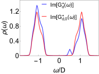
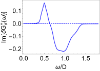
Figure 2: (Color online) Numerical calculation of electronic LDOS on the impurity site (blue) compared with the bulk (red) (2), and the variation of LDOS on the impurity(2).

Solution for multiple impurities.   The single impurity solution considered above is already the upper bound in terms of bound state energies, which are very close to the UHB. However, in the experiments for the Ca²⁺ vacancy of Ref. Ye et al. (2013), the bound state is closer to the Fermi energy. In the finite doping but still insulating casesCai et al. (2015), the binding energies of the in-gap states are way beyond this limit. They can actually approach the Fermi energy, but but never reacher it. The spectral weight of the in-gap states forms a sharply $V$-shaped feature centered at the Fermi energy. We nowshow that, by considering multiple impurities, these properties are also captured within our framework: i) bound states of similar energies superimpose to create new bound states with smaller energies; ii) such bound states carry smaller spectral weights compared to that of the single impurity case.

For simplicity, we start with the two-impurity case. We label their positions as $\bm{x}_{1}$ and $\bm{x}_{2}$, and their corresponding single-impurity $T$-matrices as $\hat{T}_{1}$ and $\hat{T}_{2}$ which are similarly defined in Eq. (13). To the lowest order, the full $T$-matrix is given by Economou (2006)

$$\hat{T}=f_{12}(\hat{T}_{1}+\hat{T}_{2}+\hat{T}_{1}g_{12}\hat{T}_{2}+\hat{T}_{2}g_{21}\hat{T}_{1}),$$ (19)

with $f_{12}=(1-t_{1}t_{2}g_{12}g_{21})^{-1},$ and $t_{i}=\nu h_{0}(\bm{x}_{i})(1-\nu h_{0}(\bm{x}_{i})g_{ii})^{-1}$. Both $\hat{T}_{1}$ and $\hat{T}_{2}$ contribute in-gap bound states at their own $\nu_{b,1(2)}$. Moreover, the factor $f_{12}$ contributes new bound states, the energies of which are deduced from

$$\begin{split}&1-t_{1}t_{2}g_{12}g_{21}=0\Rightarrow\nu_{b}=\frac{A\pm\sqrt{A^{2}-4B}}{B},\end{split}$$ (20)

where $A=h_{1}g_{11}+h_{2}g_{22}$, $B=h_{1}h_{2}(g_{11}g_{22}-g_{12}g_{21})$, and $h_{i}=h_{0}(\bm{x}_{i})$. The new bound state solutions have the following properties: i) $\nu_{b}$ cannot reach zero just as for the single impurity case; ii) the new $\nu_{b}$’s are different from $\nu_{b,1}$ or $\nu_{b,2}$; iii) the new solutions ($\nu_{b}$’s) are also positive-definite, meaning that they are also descending down from the UHB; iv) most importantly, they become smaller, i.e. closer to the Fermi energy. In the single impurity case, the value of $h_{0}$ is bounded as $\lvert\delta\mbox{$\langle n_{f}\rangle$}\rvert\leq 1$ which further puts bounds on $\nu_{b}$ from below. However, in Eq. (20), when the two impurity potentials are close enough, we have $B\ll A$. By expanding Eq. (20) in terms of small $B$, we find

$$\nu_{b}\sim 1/A=1/(h_{1}g_{11}+h_{2}g_{22}).$$ (21)

Let $h_{1}=h_{2}=h_{0}$, and $g_{11}=g_{22}=g_{00}$, and compare Eq. (21) with the single impurity case, $\nu_{b,\text{single}}\simeq g_{00}h_{0}$. Therefore, the new bound state can be considered as generated by an effective and larger $h^{\prime}_{0}\simeq 2h_{0}$. In other words, the strength of impurities close together effectively adds up to produce bound states with lower and lower energies. Similar approximation can be made by considering the $T$-matrix of $M$ impurities (see Supplement Materials), i.e. when these impurities are sufficiently close, the bound state of the lowest energy can be viewed as generated by a single impurity with all the impurity strength superimposed $h^{\prime}_{0}\simeq\sum_{m=1,\dots,M}h_{m}g_{mm}$, which The bound state energies $\nu_{b}\sim 1/h_{0}^{\prime}$ is pushed closer to the Fermi energy as the number of impurities in a cluster increases.

Therefore, we consider that the $h_{0}$ in the single impurity calculation can be tuned to larger values by nearby impurity concentration rather than bounded, and compute bound state energies and their corresponding spectral weights in the single impurity solution as a function of $h_{0}$.

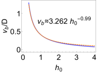
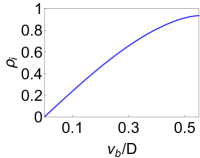
Figure 3: The bound state energies $\nu_{b}$ plotted as a function of the effective rotor impurity potential $h_{0}$ (3) and the spectral weights $\rho_{i}$ at given energy $\nu_{b}$ (3).

We plot the energies of the in-gap states $\nu_{b}$ as a function of the impurity potential strength $h_{0}$ in Fig. (3) and the corresponding spectral weights in Fig. (3). Note that the asymptotic behavior is $\nu_{b}\sim 1/h_{0}$, which forbids the impurity state from reaching zero, i.e. the Fermi energy of the bulk. The corresponding spectral weight $\rho_{i}=\frac{(\Lambda_{0}(\nu_{b})^{2}-\pi^{2}\rho_{0}(\nu_{b})^{2})}{\lvert h_{0}(\nu_{b}\ \partial_{\nu}\Lambda_{0}(\nu_{b})+\Lambda_{0}(\nu_{b}))\rvert}$ decreases when $\nu_{b}$ approaches zero.

Summary and implications.   In this work, we have studied the effect of a single impurity in the Mott insulator using a slave rotor method. We solve the rotor impurity problem using the $T$-matrix method, and find that the solution accounts for both of the key features of the observed local density of states on a single impurity regarding i) positions and amplitudes of the in-gap spectral weights; ii) the spectral weight transfer from the upper Hubbard band to the lower Hubbard band. Further analysis of solutions for multiple impurities shows that high impurity concentration can induce a larger effective impurity potential $h_{0}$ for the rotor fields.

From those results, we can explain the difference between the LDOS on the Cl^- site and the Ca²⁺ site. The LDOS of Cl^- vacancy is well explained by the single impurity solution while that of a single Ca²⁺ vacancy is much closer to the Fermi energy. To explain the discrepancy, we note that the impurity potential of a Ca²⁺ vacancy acts simultaneously on its four neighboring Cu sites (see Supplement Materials), forming a four-impurity cluster. Thus, according to our approximation for the multi-impurity case, the peak position (relative to the Fermi energy) of Ca²⁺ vacancy should be about $1/4$ of that for the Cl^- site. The experimental results in Ref. [Ye et al., 2013] give $\omega_{b}(\text{Cl}^{-})\simeq 1.8eV$ and $\omega_{b}(\text{Ca}^{2+})\simeq 0.5eV$, showing a quantitative agreement with our theory.

Our work suggests that the observed V-shaped LDOS suppression is a generic feature of Mott insulators with or without magnetism. This is manifested by the special form of the effective rotor impurity potential, $\hat{H}_{X,\bm{x}_{0}}=ih_{0}(X^{*}_{\bm{x}_{0}}\partial_{t}X_{\bm{x}_{0}}-h.c.)$ which vanishes for $\nu=0$ as long as the system is still in the Mott insulator phase.

More generally, the vanishing of LDOS reflects an exact zero of the local Green’s function of the parent Mott phase rather than just the zeros of the spectral function, as we show in the Supplement Materials. This exact zero of the local Green’s function is a consequence of the Luttinger surface of the electrons’ Green’s function in $\bm{k}$-space at the Fermi energy. In our approach, the Luttinger surface is located in $\bm{k}$-space at the spinon Fermi surface, where the spinon Green’s function has poles. These poles are turned into zeros through the convolution with the rotor’s Green’s function, which possesses a plane of zeros at $\nu=0$. We propose that this Luttinger surface has a topological stability related to the Mott gap, in a sense similar to the stability of a Fermi surfaceVolovik2009 ; Horava2005 . Exactly how such protection works is an intriguing open question for future studies.

We would like to acknowledge useful discussions with Y. Y. Wang. This work was in part supported by the the NSF Grant No. DMR-1611392, U.S. Army Research Office Grant No. W911NF-14-1-0525, and the Robert A. Welch Foundation Grant No. C-1411(S.E.G. and Q.S.). Q.S. acknowledges the support of ICAM and a QuantEmX grant from the Gordon and Betty Moore Foundation through Grant No. GBMF5305 (Q.S.), the hospitality of University of California at Berkeley and of the Aspen Center for Physics (NSF grant No. PHY-1607611), and the hospitality and support by a Ulam Scholarship of the Center for Nonlinear Studies at Los Alamos National Laboratory.

Supplemental Materials

Slave Rotor Approach to Mott Insulators:   Using $\partial_{t}\theta_{i}=X_{i}^{*}\partial_{t}X_{i}$, we obtain the following Lagrangian from the original Hubbard model Hamiltonian:

$$\begin{split}&\mathcal{L}_{HM}=\sum_{i,\alpha}f^{\dagger}_{i\alpha}(-i\partial_{t}+h_{i})f_{i\alpha}+\sum_{i}\Big{(}\frac{-\lvert\partial_{t}X_{i}\rvert^{2}}{U}\\ &+\frac{h_{i}}{U}(X_{i}^{*}\partial_{t}X_{i}-X_{i}\partial_{t}X_{i}^{*})+\lambda_{i}(\lvert X_{i}\rvert^{2}-1)\Big{)}\\ &+\sum_{ij,\alpha}(t_{ij}f^{\dagger}_{i,\alpha}f_{j,\alpha}X_{i}X^{*}_{j}+h.c.).\end{split}$$ (S-1)

Note that $\frac{U}{2}\sum_{i}\hat{L}_{i}^{2}=\frac{-\lvert\partial_{t}X_{i}\rvert^{2}}{2U}$; we have rescaled $U$ to $U/2$ in (S-1) to preserve the correct atomic limitFlorens and Georges (2002). Here, $h_{i}$ and $\lambda_{i}$ are two Lagrangian multipliers to enforce the two constraints that were described in the main text.

The spinon-boson coupling term is decoupled via

$$Q_{f,ij}=\mbox{$\langle X_{j}^{*}X_{i}\rangle$},\qquad Q_{X,ij}=\mbox{$\langle\sum_{\alpha}f_{j\alpha}^{\dagger}f_{i\alpha}\rangle$}.$$ (S-2)

The Lagrangian $\mathcal{L}_{HM}$ is expressed in two parts:

$$\mathcal{L}_{MF,f}=\sum_{i,\alpha}(f^{\dagger}_{i\alpha}(-i\partial_{t}+h_{i})f_{i\alpha}+t\sum_{\mbox{$\langle ij\rangle$},\alpha}(Q_{f}f^{\dagger}_{i\alpha}f_{j\alpha}+h.c.),$$ (S-3)

$$\begin{split}\mathcal{L}_{MF,X}&=\sum_{i}\Big{(}\frac{-\lvert\partial_{t}X_{i}\rvert^{2}}{U}+\frac{h}{U}(X_{i}^{*}\partial_{t}X_{i}-X_{i}\partial_{t}X_{i}^{*})\\ &+\lambda_{i}\lvert X_{i}\rvert^{2}\Big{)}+t\sum_{\mbox{$\langle ij\rangle$}}(Q_{X}X_{i}X^{*}_{j}+h.c.).\end{split}$$ (S-4)

A saddle-point solution arises when one generalizes each $X_{i}$ to $M$ species so that its symmetry becomes $O(2M)$, scales the hoping $t_{ij}$ to $1/M$, and takes the large (N,M) limit with a fixed ratio $M/N$ Florens and Georges (2004); Lee and Lee (2005). In our analysis, we express our equations for $N=2M=2$.

Calculation of the constraint:   The electron density is given by $\mbox{$\langle\sum_{\sigma}d^{\dagger}_{\sigma}d_{\sigma}\rangle$}=\mbox{$\langle\sum_{\sigma}f^{\dagger}_{\sigma}f_{\sigma}\rangle$}$, and the rotor fields are constrained by $\mbox{$\langle\hat{L}\rangle$}=\mbox{$\langle U^{-1}(-i\partial_{t}\theta+h)\rangle$}=\mbox{$\langle\sum_{\sigma}f^{\dagger}_{\sigma}f_{\sigma}-1/2\rangle$}$. To enforce the constraints, we need to first compute $\langle\hat{L}\rangle$ at finite $h$. Since $X_{i}=e^{i\theta_{i}}$, we have $\theta_{i}=-i\ln X_{i}$, therefore, $-i\partial_{t}\theta_{i}=-X_{i}^{*}\partial_{t}X_{i}$, and

$$\hat{L}=(-X_{i}^{*}\partial_{t}X_{i}+h)/U.$$ (S-5)

We compute $\langle\hat{L}\rangle$ using the functional integral in the $X$-field representation and find

$$\begin{split}&\mbox{$\langle\hat{L}\rangle$}=h/U-\frac{h/2}{\sqrt{-h^{2}+\lambda U}}.\end{split}$$ (S-6)

When there is no doping, it follows from Eq. (2) that $\mbox{$\langle\hat{L}\rangle$}=0$.

Experimental measurements. Experimental results of the impurity LDOS in cuprate parent compounds are reproduced in Fig. (S1).

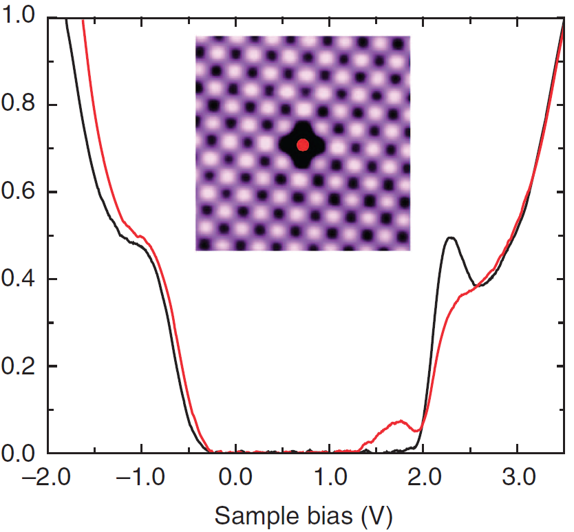
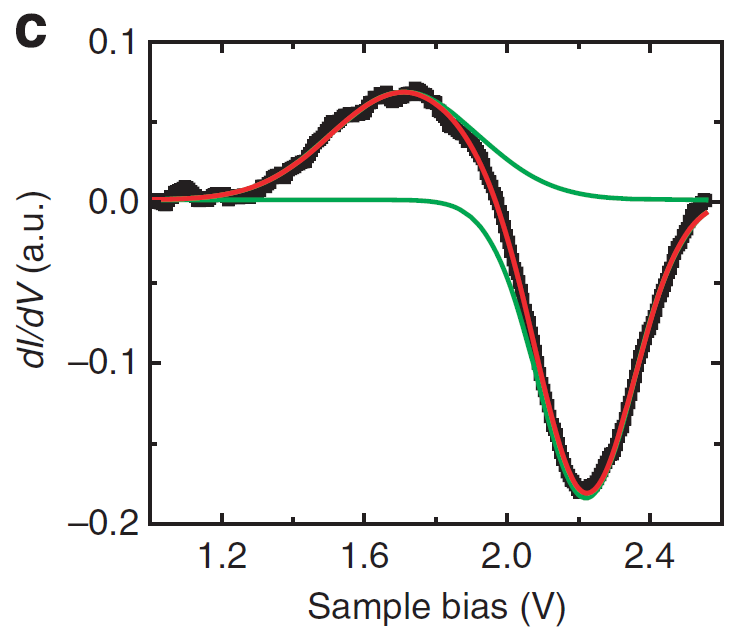
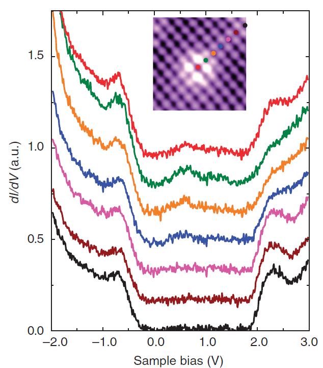
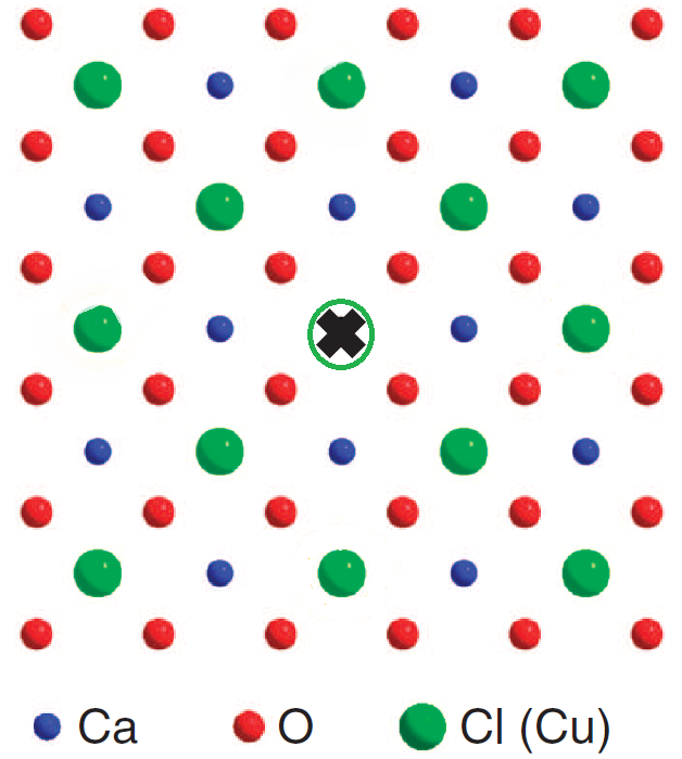
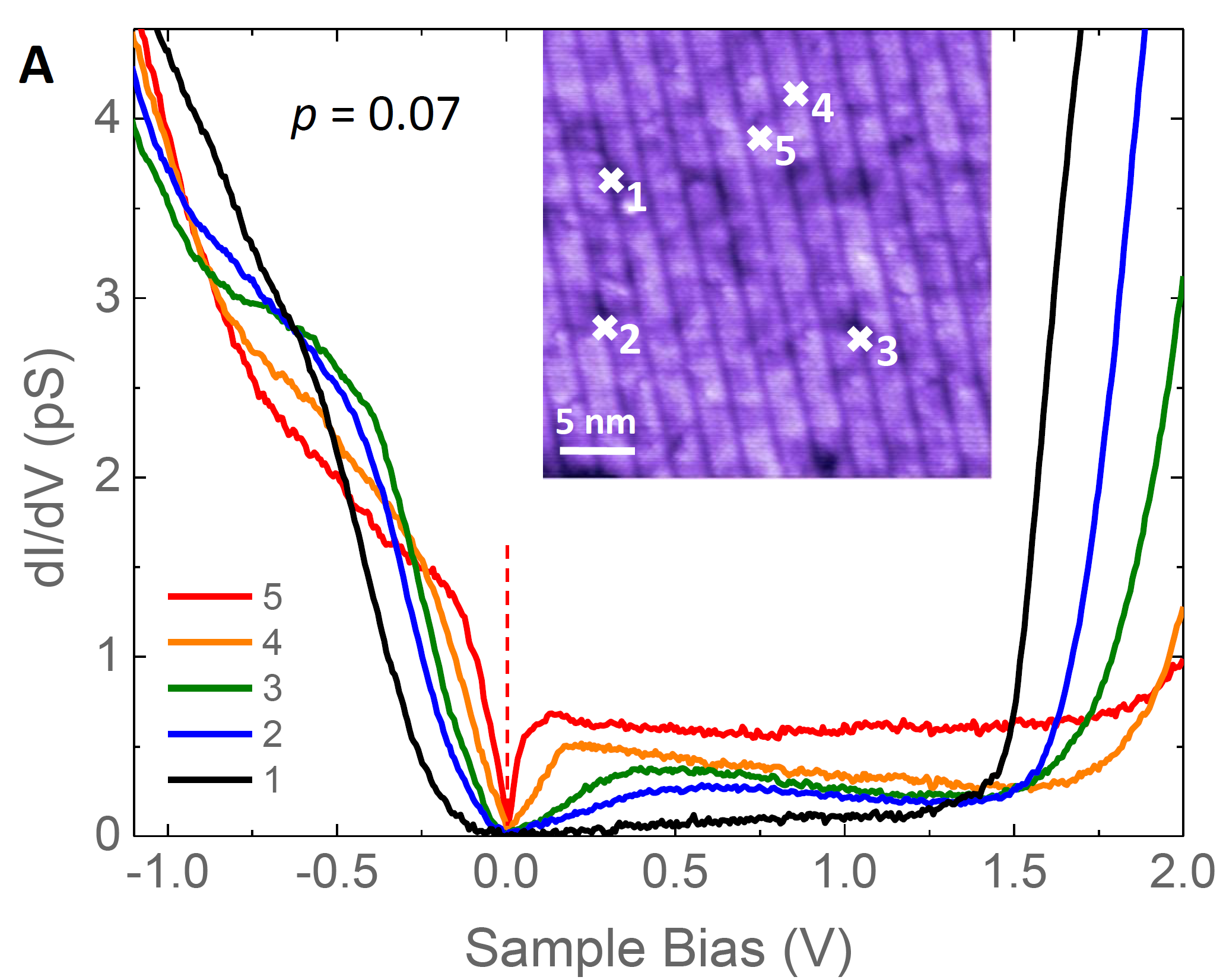
Figure S1: (a) Single impurity LDOS (red) compared with the bulk LDOS (black). The single impurity corresponds to a Cl^- vacancy. (b) Difference of LDOS between the impurity site and the bulk state. (c) Measurement on a Ca²⁺ vacancy, where the potential effectively forms a four-impurity cluster. The bound state occurs at energy much closer to the Fermi energy compared to that of the Cl^- vacancy in (a). (d) Schematic topview of exposed surface showing the missing Cl defect (dark cross) which is on top of a Cu atom (green circle). (e) Schematic top view showing the position of the Ca-site defect (dark dot) and the nearest-neighbour Cu sites (orange circles). (f) The LDOS of a 7% doping sample which shows a sharp “V”-shaped dip.

Multi-impurity T-matrix:   Consider $M$ impurities labeled by $\bm{x}_{m}$ with $m=1,2,\dots,M$. The T-matrix is now given by

$$\hat{T}=(I_{M}-\hat{V}\hat{\Gamma})^{-1}\hat{V},$$ (S-7)

where $I_{M}$ is an identity matrix of dimension $M\times M$, $\hat{V}$ is a diagonal matrix with elements $V_{mm}=h_{0}(\bm{x}_{m})$, and $\hat{\Gamma}_{ij}=g_{ij}$ with $\bm{x}_{i(j)}$ belonging to the impurity sites. The new poles are solved from $\det[I_{M}-\hat{V}\hat{\Gamma}]=0$. By keeping to second order terms ($\sim\mathcal{O}(\nu^{2})$), we find $\nu_{b}\sim(\sum_{m}h_{m}g_{mm})^{-1}$ with $\bm{x}_{m}$ denoting positions of the impurities.

Probing the zero of local Green’s function:   To further shed light on interpretation of the experimental results, we propose that we can interpret the impurity LDOS as a measurement of the local and energy resolved compressibility of the bulk state as follows. The local impurity potential distribution of $\mu_{imp}(\bm{x})$ within a sample can be viewed as an ensemble of source fields $\{\delta\mu(\bm{x}_{0})\}$ that couples to the density operator. Then $\rho^{imp}(\omega;\bm{x})$ is equivalent to $\rho(\omega;\bm{x};\{\delta\mu(\bm{x}_{0})\})$, the LDOS in the presence of a source field ensemble $\{\delta\mu(\bm{x}_{0})\}$. Theorerically, we consider the source field ensemble $\{\delta\mu(\bm{x}_{0})\}$ tunable. Experimentally, the system is well within the Mott insulating phase, and no phase separation appears. Therefore, the variation of LDOS due to the source fields:

$$\delta\rho(\omega;\bm{x};\{\delta\mu(\bm{x}_{0})\})=\rho(\omega;\bm{x};\{\delta\mu(\bm{x}_{0})\})-\rho^{bulk}(\omega;\bm{x})$$ (S-8)

can be further considered as linear response, i.e. we can take the zero source limit $\{\delta\mu(\bm{x}_{0})\}\rightarrow 0$. Such linear response can be formally expressed as:

$$\begin{split}&\left.\frac{\delta\rho(\omega;\bm{x};\{\delta\mu(\bm{x}_{0})\})}{\{\delta\mu(\bm{x}_{0})\}}\right|_{\{\delta\mu(\bm{x}_{0})\}\rightarrow 0}=\frac{\delta\rho^{bulk}(\omega;\bm{x})}{\delta\mu},\end{split}$$ (S-9)

and the measured LDOS variation is expressed as

$$\delta\rho(\omega;\bm{x};\{\delta\mu(\bm{x}_{0})\})\simeq\frac{\delta\rho^{bulk}(\omega;\bm{x})}{\delta\mu}\times\{\delta\mu(\bm{x}_{0})\}.$$ (S-10)

Therefore, the key experimental observation that no spectral weight of LDOS in the presence of impurities is allowed at $\omega=0$ can be viewed as

$$\frac{\delta\rho^{bulk}(\omega=0;\bm{x})}{\delta\mu}=0,$$ (S-11)

as $\{\delta\mu(\bm{x}_{0})\}$ is arbitrary (within the linear response region).

Then we can further transform $\frac{\delta\rho^{bulk}(\omega;\bm{x})}{\delta\mu}$ as

$$\frac{\delta\rho^{bulk}(\omega;\bm{x})}{\delta\mu}=\frac{\partial\rho^{bulk}(\omega;\bm{x})}{\partial\mu}(-\frac{\delta\Sigma(\omega;x)}{\delta\mu}-1),$$ (S-12)

where $\Sigma(\omega;x)$ is the local electronic Dyson self-energy. Assuming that

$$(-\frac{\delta\Sigma(\omega=0;x)}{\delta\mu}-1)\neq 0$$

which is generally true, the vanishing of the LDOS means that

$$\frac{\partial\rho^{bulk}(\omega=0;\bm{x})}{\partial\mu}=0.$$ (S-13)

Then we can write the real part of the Green’s function through the Hilbert transform as

$$\Re e[G(\omega;\bm{x})]=\mathcal{P}\int d\omega^{\prime}\frac{\rho^{bulk}(\omega^{\prime};\bm{x})}{\omega-\omega^{\prime}}.$$ (S-14)

Taking $\omega=0$, the integral on the right hand side is completely determined by the $\omega^{\prime}=0$ contribution as the contribution from finite $\omega^{\prime}$ cancels due to dynamic particle-hole symmetry of the bulk state spectral function $\rho^{bulk}(-\omega^{\prime};\bm{x})=\rho^{bulk}(\omega^{\prime};\bm{x})$ (which is only true at half filling)

$$\begin{split}&\Re e[G(\omega=0;\bm{x})]=-\mathcal{P}\int d\omega^{\prime}\frac{\rho^{bulk}(\omega^{\prime};\bm{x})}{\omega^{\prime}}\\ &=-\frac{\partial\rho^{bulk}(\omega^{\prime};\bm{x})}{\partial\omega^{\prime}}|_{\omega^{\prime}\rightarrow 0}\\ &\propto\frac{\partial\rho^{bulk}(\omega=0;\bm{x})}{\partial\mu}=0,\end{split}$$ (S-15)

where in the last line we used the relation

$$\frac{\partial\rho^{bulk}(\omega;\bm{x})}{\partial\mu}\propto\frac{\partial\rho^{bulk}(\omega;\bm{x})}{\partial\omega}$$

as $\mu$ only explicitly shows up in electronic Green’s function as

$$G(\omega;\bm{x})=\int d^{2}\bm{k}\frac{e^{i\bm{k}\cdot\bm{x}}}{\omega-\mu-\epsilon_{\bm{k}}-\Sigma(\omega;\bm{k})}.$$ (S-16)