Quadrupole moments of spin–1 systems: the $\rho$ meson, the $S$–wave deuteron and some general constraints

Abstract

We costruct the relativistic operator of the quadrupole moment of two-particle composite spin one systems with zero orbital moment of the relative motion and derive explicit analytical expression for the quadrupole moment using the approach to relativistic composite systems based on our version of the instant-form relativistic quantum mechanics (RQM). We calculate the quadrupole moments of the $\rho$ meson and of the $S$-wave deuteron without any free parameters, using our unified $\pi$&$\rho$ model (Phys. Rev.D 93, 036007 (2016); 97, 033007 (2018)) and our previous results on deuteron. Our calculation gives $Q_{\rho}=-0.158\pm 0.04$ GeV^-2 and $Q_{d}=-1.4\cdot 10^{-4}$ GeV^-2. Having in our disposition the rather general form of the quadrupole-moment operator we for the first time formulate the problem of the upper and lower bounds for possible values of the quadrupole moment of a two-particle system with indicated quantum numbers for a large range of constituent masses, and partially solve it.

I Introduction

The electroweak properties of hadrons (decay constants, mean square radii, static moments, electromagnetic form factors etc.) are of fundamental importance for the understanding of strong interactions at low and intermediate energy scales. So, it is clear that the theory of such properties based on different nonperturbative approaches is in the focus of investigations for years. Let us mention for example different forms of Dirac relativistic dynamics BaE85 ; CaG95 ; ChC88 ; MeF97 ; CaD98 ; BaC02 ; Jau03 ; ChJ04 ; HeJ04 ; BiS14 ; MeS15 ; SuD17 , approaches based on the Dyson-Schwinger equation HaP99 ; BhM08 ; RoB11 ; PiS13 , the Nambu-Jona-Lasinio model CaB15 ; LuC15 , QCD sum rulesSam03 ; AlO09 , the light front diagram technique MeS02 , lattice calculations AnW97 ; HeK07 ; OwK15 ; LuS16 . The quadrupole moment of two-particle spin one systems with total electric charge equal to unity with $S$-state of the relative motion of constituents is of particular interest because the existence of the quadrupole form factor and the quadrupole moment in such systems is a purely relativistic effect. They are strictly zero in the non-relativistic case. The actual cause of the effect is well known (see, e.g., the textbook Nov75 ): the relativistic spin rotation of the constituents. This effect is a kinematic one, and so it must show itself in all composite systems with given quantum numbers, being independent from the nature of constituents and the kind of their interaction. In particular, this effect takes place in two well studied systems with principally different constituents and types of the interaction: the $\rho$ meson and the deuteron. It is worth noting that a kind of universal conditions for the quadrupole moment of such systems was given in the well known paper BrH92 .

The results of calculations of $\rho$-meson the quadrupole moment through different approaches (see, e.g.,  BaE85 ; CaG95 ; MeF97 ; CaD98 ; BaC02 ; Jau03 ; ChJ04 ; HeJ04 ; BiS14 ; CaB15 ; MeS02 ) differ essentially not only in the absolute value but even in sign. To-day it is not possible to estimate the credibility of these results because the experimental data on the $\rho$ meson are scarce. Its lifetime is very short, so direct measurements of its electroweak properties are nearly impossible.

Although the deuteron quadrupole moment is measured with great accuracy (see, e.g., GaO01 ; GiG02 ), it is clear that the quadrupole form factor and the quadrupole moment of the deuteron are mainly defined by the $D$-wave part of the deuteron wave function. The $S$-state admixture is small and it is very difficult to separate it. The contribution of the pure $S$-state to the quadrupole moment is relatively small and it is doubtful whether it can be extracted from the experiment.

The goal of the present paper is threefold. First, we derive an explicit analytic formula for the quadrupole moment $Q$ of a two-particle spin one system in the $S$-state of relative motion of constituents. Second, we calculate the quadrupole moments of the $\rho$ meson and the $S$-wave deuteron using no free parameters. Third, in the framework of our relativistic approach we obtain some general constraints for possible values of the quadrupole moment in two-particle systems with quantum numbers given above for a large range of constituent masses from $\rho$ meson to deuteron.

The approach that we use in the present paper is a particular relativistic formulation of constituent-quark model that is based on the classical paper by P. Dirac Dir49 (so-called Relativistic Hamiltonian Dynamics or Relativistic Quantum Mechanics (RQM)). RQM can be formulated in different ways or in different forms of dynamics. The main forms are instant form (IF), point form (PF) and light-front (LF) dynamics. The properties of different forms of RQM dynamics can be found in the reviews LeS78 ; KeP91 ; Coe92 ; KrT09 . Today the approach is largely used for nonperturbative theory of particle structure.

Here we use our version of RQM, – the modified instant form (mIF) of RQM , that was successfully used for various composite two-particle systems, namely, the deuteron KrT07 , the pion KrT01 ; KrT98 ; KrT09prc ; TrT13 , the $\rho$ meson KrP16 ; KrP18 and the kaon KrT17 . This model has predicted with surprising accuracy the values of the form factor $F_{\pi}(Q^{2})$, which were measured later in JLab experiments Vol01 ; Hor06 ; Tad07 ; Blo08 ; Hub08 (see discussion in Ref. KrT09prc ). All the new points fall, within the experimental uncertainties, on the initially calculated curve. Another advantage of the approach is matching with the QCD predictions in the ultraviolet limit: when constituent-quark masses are switched off, as expected at high energies, the model reproduces correctly not only the functional form of the QCD asymptotics, but also its numerical coefficient; see Refs. KrT98 ; TrT13 ; TrT15 for details. The method allows for an analytic continuation of the pion electromagnetic form factor from the spacelike region to the complex plane of momentum transfers and gives good results for the pion form factor in the timelike region KrN13 .

Now we use this approach, supplemented with some physical reasoning based on the consideration of the structure of our relativistic operator of the quadrupole moment, to obtain some constraints for possible values of the quadrupole moment of two-particle spin one systems in the $S$-state of relative motion. The effectiveness of our approach for a relativistic theory of two-particle composite systems permits us to believe that our constraints are of a rather general character.

In what concerns the calculation of the quadrupole moment of the $\rho$ meson, the present paper is a continuation of our papers KrP16 ; KrP18 . Using our approach we have constructed KrP16 the unified $\pi$&$\rho$ model and have fixed all free parameters determining the radius of the $\rho$ meson through its decay constant. Then we obtain the $\rho$ meson magnetic moment $\mu_{\rho}$ KrP18 using the unified $\pi$&$\rho$ model with no new fitting parameters. Now we calculate the $\rho$-meson quadrupole moment in the unified $\pi$&$\rho$ model, that is without any fitting parameters: all parameters are already fixed in KrP16 .

The reliability of our calculation of the quadrupole moment of the $S$-wave deuteron in our approach is based on the results of the paper KrT07 where very good theoretical results were derived for the electromagnetic properties of the deuteron obtained in polarization experiment on the electron-deuteron scattering, that is for the component $T_{20}(Q^{2})$ of the deuteron polarization tensor and for its quadrupole form factor. In the present paper we use the $S$-component of the deuteron wave function KrT07MT , that was constructed in the framework of the so-called potentialless formulation of the inverse scattering problem MuT81 (see also Tro94 ).

Our relativistic operator of the quadrupole moment of the two-particle system constructed in the basis of state-vectors with the motion of center-of-mass being separated is a c-number function. To obtain some general results for arbitrary constituents with spin 1/2 in the $S$-state of relative motion we divert our attention away from the fixed parameters in unified $\pi$&$\rho$ model or in the deuteron wave function. Now we consider the operator of the quadrupole moment on the class of parameters that characterize, on the one hand, the constituents (the mass, the anomalous magnetic moments) and, on the other hand, the interaction of constituents. We consider weak interactions (as in deuteron), intermediate model interaction (see, e.g., KrT01 ; KrP18 ) and strong interactions that ensure square-law quark confinement (harmonic oscillator wave function).

The derived expression for the relativistic quadrupole-moment operator suggests that one can obtain some general limitations for the values of quadrupole moment of systems under consideration. The analysis of the formula for the quadrupole-moment operator, some additional physical reasoning and involvement of numerical calculations enable us to construct the upper and lower bounds for the values of quadrupole moments under consideration, resulting in some constraints.

The rest of the paper is organized as follows. In Sec. II, the quadrupole form factor and the quadrupole moment of a spin one two-particle system in the $S$-state of the relative motion are derived in modified impulse approximation of IF RQM. In Sec. III we calculate the values of quadrupole moments of the $\rho$ meson (using the unified $\pi$&$\rho$ model with no free parameters) and of the deuteron in $S$-state with no $D$-wave admixture. Sec. IV contains the analysis of the properties of the relativistic quadrupole-moment operator for indicated quantum numbers and of the dependence of its value on the model interaction of constituents as well as on the values of constituent masses and anomalous magnetic moments. In Sec. V general limitations for the values of the quadrupole moment of different systems with mentioned quantum numbers are proposed and discussed. We briefly conclude in Sec.VI and present some details of the calculation in the Appendix.

II The quadrupole moment of $S$-state two-particle
spin one system as a relativistic effect

One of the main points of our approach is the construction of matrix element of electromagnetic current for a composite system of two interacting particles. A summary of our method of such construction can be found in our recent paper KrP18 and in the references therein. The method is based on the principal statements of RQM dynamics(see, e.g., BaT53 ) and on the general procedure of relativistic covariant construction of local operators matrix elements ChS63 .

Let us consider a system of two interacting particles of the mass $M$, the spin 1/2 and the total electric charge 1 in the $S$-state of relative motion. In RQM the basis of individual spins and momenta of particles can be used

$$\left|\,\vec{p}_{1}\,,m_{1};\vec{p}_{2}\,,m_{2}\rangle\right.=\left|\,\vec{p}_{1}\,,m_{1}\rangle\otimes|\vec{p}_{2}\,,m_{2}\rangle\right.\;,$$ (1)

where $\vec{p}_{1,2}$ are the constituent momenta and $m_{1,2}$ are their spin projections. One can also choose the following set of two-particle state vectors where the motion of the center of mass is separated:

$$|\,\vec{P},\;\sqrt{s},\;J,\;l,\;S,\;m_{J}\,\rangle\;,$$ (2)

where $P_{\mu}=(p_{1}+p_{2})_{\mu}$, $P^{2}_{\mu}=s$; $\sqrt{s}$ is the invariant mass of the two-particle system, $l$ is the orbital angular momentum in the center-of-mass frame (C.M.S.), $\vec{S}\,^{2}=(\vec{S}_{1}+\vec{S}_{2})^{2}=S(S+1)\;,\;S$ is the total spin in C.M.S., $J$ is the total angular momentum with the projection $m_{J}$. The two-particle basis with separated motion of the center of mass (2) is connected with the basis of individual spins and momenta of two particles (1) through the appropriate Clebsh-Gordan decomposition for the Poincaré group (see, e.g., KrT09 ).

The current matrix element for our system is

$$\langle\vec{p}_{c}\,,m_{Jc}|j_{\mu}(0)|\vec{p}_{c}\,^{\prime}\,,m^{\prime}_{Jc}\rangle\;,$$ (3)

where $\vec{p}_{c}\;,\;\vec{p}_{c}\,^{\prime}$ are the momenta of composite two-particle system in initial and final states, respectively, $m_{Jc}\;,m^{\prime}_{Jc}$ are projections of the total angular momenta. As the expression (3) is a matrix in the projections of the total angular momentum, it can be decomposed in the sum of linearly independent matrices (see for detail KrT09 ; KrP18 ; ChS63 ) that presents a set of $2J+1$ independent Lorentz scalars (that is scalars or pseudoscalars):

$$D^{J_{c}}(p_{c},p^{\prime}_{c})\left(p_{c\mu}\Gamma^{\mu}\left(p^{\prime}_{c}\right)\right)^{n}\;,\quad n=0,1,2,\ldots,2J\;,$$ (4)

here $D^{J}$ is the matrix of Wigner rotation (see, e.g., Nov75 ). The spin 4-vector $\Gamma^{\mu}$ KrT09 ; ChS63 is defined as follows:

$$\Gamma_{0}(p_{c})=(\vec{p}_{c}\vec{J})\;,\quad\vec{\Gamma}(p_{c})=M_{c}\,\vec{J}_{c}+\frac{\vec{p}_{c}(\vec{p}_{c}\vec{J}_{c})}{{p_{c}}_{0}+M_{c}}\;,$$

$$\quad\Gamma^{2}=-M_{c}^{2}\,J_{c}(J_{c}+1)\;.$$ (5)

In the decomposition of (3) in terms of the set (4) each Lorentz scalar is multiplied by a 4-vector constructed of variables that enter the state vectors in initial and finite states. So, the decomposition has the form (see also KrP18 ; KrT03 ):

$$\langle\vec{p}_{c}\,,\,m_{Jc}|j_{\mu}(0)|\vec{p}_{c}\,^{\prime}\,,\,m^{\prime}_{Jc}\rangle=$$

$$\langle\,m_{Jc}|\,D^{1}(p_{c}\,,\,p^{\prime}_{c})\,\sum_{i=1,3}\,\tilde{\cal F}\,^{i}_{c}(t)\,\tilde{A}^{i}_{\mu}\,|m^{\prime}_{Jc}\rangle\;,$$

$$\tilde{\cal F}\,^{1}_{c}(t)=\tilde{f}^{c}_{10}+\tilde{f}^{c}_{12}\left\{[i{p_{c}}_{\nu}\,\Gamma^{\nu}(p^{\prime}_{c})]^{2}\right.\left.\right.-$$

$$\left.\frac{1}{3}\,\hbox{Sp}[i{p_{c}}_{\nu}\,\Gamma^{\nu}(p^{\prime}_{c})]^{2}\right\}\frac{2}{\hbox{Sp}[{p_{c}}_{\nu}\,\Gamma^{\nu}(p^{\prime}_{c})]^{2}}\;,$$ (6)

$$\tilde{\cal F}\,^{3}_{c}(t)=\tilde{f}^{c}_{30}\;,$$

$$\tilde{A}^{1}_{\mu}=(p_{c}+p^{\prime}_{c})_{\mu}\;,\quad\tilde{A}^{3}_{\mu}=\frac{i}{M_{c}}\varepsilon_{\mu\nu\lambda\sigma}\,p_{c}^{\nu}\,p^{\prime}_{c}\,{}^{\lambda}\,\Gamma^{\sigma}(p^{\prime}_{c})\;.$$

Here $M_{c}$ is the mass of composite system, $Q^{2}=-q^{2}=t$, $q$ - 4-vector of the momentum transfer, $\tilde{f}^{c}_{10}\,,\,\tilde{f}^{c}_{12}\,,$ $\tilde{f}^{c}_{30}$ are the charge, quadrupole and magnetic form factors, respectively.

The invariant parts that one can extract from the matrix element are called the Sachs form factors of the composite system. One have the charge $G_{C}(Q^{2})$, quadrupole $G_{Q}(Q^{2})$ and magnetic $G_{M}(Q^{2})$ form factors (see, e.g., BrH92 ; ArC80 ). The Sachs form factors can be written in terms of the form factors in (6) as follows:

$$G_{C}(Q^{2})=\tilde{f}^{c}_{10}(Q^{2})\;,\quad G_{Q}(Q^{2})=\frac{2\,M_{c}^{2}}{Q^{2}}\,\tilde{f}^{c}_{12}(Q^{2})\;,$$

$$\quad G_{M}(Q^{2})=-\,M_{c}\,\tilde{f}^{c}_{30}(Q^{2})\;.$$ (7)

The current matrix element in RQM (3) can be decomposed in the complete set of states (2):

$$\langle\vec{p}_{c}\,,\,m_{Jc}|j_{\mu}(0)|\vec{p}_{c}\,^{\prime}\,,\,m^{\prime}_{Jc}\rangle=$$

$$\sum\limits_{m_{J}}\int\frac{d\vec{P}\,d\vec{P}\,^{\prime}}{N_{CG}N^{\prime}_{CG}}d\sqrt{s}\,d\sqrt{s^{\prime}}\langle\vec{p}_{c}\,,\,m_{Jc}|\,\vec{P}\,,\,\sqrt{s}\,,\,m_{J}\,\rangle$$

$$\langle\vec{P}\,,\,\sqrt{s}\,,\,m_{J}\,|j_{\mu}(0)|\vec{P}\,^{\prime}\,,\,\sqrt{s^{\prime}}\,,\,m^{\prime}_{J}\,\rangle$$

$$\langle\,\vec{P}\,^{\prime}\,,\,\sqrt{s^{\prime}}\,,\,m^{\prime}_{J}|\vec{p}_{c}\,^{\prime}\,,\,m^{\prime}_{Jc}\rangle\;,$$ (8)

We do not use in the present paper the explicit form of the normalization constant $N_{CG}$ of the vectors (2) (it can be found in KrT09 ); $\langle\,\vec{P},\sqrt{s},m_{J}|\vec{p}_{c},m_{Jc}\rangle$ is the wave function of the composite system in the sense of RQM in the representation defined by the basis (2). In the state vectors in (2) the fixed quantum numbers $J=S=1\;,\;l=0$ are omitted.

The wave function of the composite system in (8) is:

$$\langle\,\vec{P}\,,\,\sqrt{s}\,,\,m_{J}|\vec{p}_{c}\,,\,m_{Jc}\rangle=N_{C}\,\delta(\vec{P}-\vec{p}_{c})\,\delta_{m_{J}m_{Jc}}\varphi(s)\;,$$ (9)

where $N_{C}$ is the normalization constant (see KrT09 ) that we do not need here.

The wave function of the relative motion $\varphi(s)$ in the representation defined by the basis (2) for $l=0\,,\,S=1$ is a solution of the eigenvalue problem for the mass (or the mass square) operator for two-particle system with interaction: $\hat{M_{I}}=\hat{M_{0}}+\hat{V}$, where $\hat{M_{0}}$ is the mass operator for two-particle system without interaction and $\hat{V}$ is the interaction operator. The wave function has the form

$$\varphi(s)=\sqrt[4]{s}\,k\,u(k)\;,\quad s=4(k^{2}+M^{2})\;,\quad\int\limits_{0}^{\infty}dk\,k^{2}\,u^{2}(k)=1\;,$$ (10)

with $M$ being the individual mass of a constituent.

Taking into account (9) we rewrite the decomposition (8) in the form:

$$\langle\vec{p}_{c}\,,\,m_{Jc}|j_{\mu}(0)|\vec{p}_{c}\,^{\prime}\,,\,m^{\prime}_{Jc}\rangle=$$

$$\int\frac{N_{C}\,N^{\prime}_{C}}{N_{CG}\,N^{\prime}_{CG}}d\sqrt{s}\,d\sqrt{s^{\prime}}\varphi(s)$$

$$\langle\vec{p}_{c}\,,\,\sqrt{s}\,,\,m_{Jc}|j_{\mu}(0)|\vec{p}_{c}\,^{\prime}\,,\,\sqrt{s^{\prime}}\,,\,m^{\prime}_{Jc}\,\rangle\,\varphi(s^{\prime})\;.$$ (11)

The matrix element in (11)

$$\frac{N_{C}\,N^{\prime}_{C}}{N_{CG}N^{\prime}_{CG}}\langle\vec{p}_{c}\,,\,\sqrt{s}\,,\,m_{Jc}|j_{\mu}(0)|\vec{p}_{c}\,^{\prime}\,,\,\sqrt{s^{\prime}}\,,\,m^{\prime}_{Jc}\,\rangle$$ (12)

is a regular Lorentz-covariant generalized function (distribution) that has a meaning only under the integral in (11). So, the integral (11) is to be regarded as a functional defined on the space of test functions $\varphi(s)\varphi(s^{\prime})$.

Now we decompose the matrix element (12) in the r.h.s.of (11) in the system of independent Lorentz-scalars (4) in analogy to (6):

$$\frac{N_{C}\,N^{\prime}_{C}}{N_{CG}N^{\prime}_{CG}}\langle\vec{p}_{c}\,,\,\sqrt{s}\,,\,m_{Jc}|j_{\mu}(0)|\vec{p}_{c}\,^{\prime}\,,\,\sqrt{s^{\prime}}\,,\,m^{\prime}_{Jc}\,\rangle=$$

$$\langle\,m_{Jc}|\,D^{1}(p_{c}\,,\,p^{\prime}_{c})\,\sum_{i=1,3}\,{\cal F}\,^{i}(s,Q^{2},s^{\prime})\,B^{i}_{\mu}(s,Q^{2},s^{\prime})\,|m^{\prime}_{Jc}\,\rangle\;,$$

$${\cal F}\,^{1}(s,Q^{2},s^{\prime})=G_{10}(s,Q^{2},s^{\prime})+$$

$$G_{12}(s,Q^{2},s^{\prime})\left\{[i{p_{c}}_{\nu}\,\Gamma^{\nu}(p^{\prime}_{c})]^{2}\right.\left.\right.-$$

$$\left.\frac{1}{3}\,\hbox{Sp}[i{p_{c}}_{\nu}\,\Gamma^{\nu}(p^{\prime}_{c})]^{2}\right\}\frac{2}{\hbox{Sp}[{p_{c}}_{\nu}\,\Gamma^{\nu}(p^{\prime}_{c})]^{2}}\;,$$ (13)

$${\cal F}\,^{3}(s,Q^{2},s^{\prime})=G_{30}(s,t,s^{\prime})\;,$$

where $B^{i}_{\mu}(s,t,s^{\prime})\;,\;i=1,3$ are some 4-vectors that are smooth functions of the variables $s,s^{\prime}$ .

Substituting of the decompositions (6), (13) in (11) and equating the expressions that stand at the equal degrees of the scalars (4) we obtain some equalities for the 4-vectors. These equalities are to be hold in the sense of Lorentz-covariant generalized functions, that is for arbitrary test functions $\varphi(s)\varphi(s^{\prime})$. This condition means that these covariant relations are to be valid for arbitrary model of the interaction of constituents in RQM. So. the vectors $B^{i}_{\mu}(s,t,s^{\prime})\;,\;i=1,3$ in (13) are the same as $\tilde{A^{i}_{\mu}}$ in (6). As a result we obtain for the invariant parts of the matrix element (3):

$$\tilde{f}^{c}_{in}(Q^{2})=\int\,d\sqrt{s}\,d\sqrt{s^{\prime}}\,\varphi(s)\,G_{in}(s,Q^{2},s^{\prime})\varphi(s^{\prime})\;.$$ (14)

The form factors $G_{in}(s,Q^{2},s^{\prime})$ are the reduced matrix elements on the Poincaré group that are given by regular Lorentz-covariant generalized functions with test functions $\varphi(s)\varphi(s^{\prime})$.

In general, the explicit form of the functions $G_{in}(s,Q^{2},s^{\prime})$, is unknown. To calculate these functions we propose a modified impulse approximation (MIA) KrT09 . In contrast to the generally accepted impulse approximation, we formulate MIA in terms of reduced matrix elements on the Poincaré group (form factors) extracted from the current matrix element and not in terms of current operators themselves. The standard impulse approximation is known to break the Lorentz-covariance and the conservation law for the composite-system electromagnetic current (see, e.g., GiG02 ; KeP91 ; KrT09 ). Note that when deriving (14) we have made no assumptions about the structure of the operator in (3), so that the Lorentz-invariance and the conservation law were not broken. MIA means that the form factors $G_{in}(s,Q^{2},s^{\prime})$ are changed for the free two-particle form factors $g_{0i}(s\,,Q^{2}\,,s^{\prime})\;,\;i=C,Q,M$ of the system with no interaction between components and with the same quantum numbers $J=S=1\,,\,l=0$.

The free two-particle form factors also are regular Lorentz-covariant generalized functions, so that the static limit of, e.g., $g_{0i}(s\,,Q^{2}\,,s^{\prime})$ is to be considered in the weak sense. The result for the quadrupole form factor of our system in MIA has the following form:

$$G_{Q}(Q^{2})=\frac{2M_{c}^{2}}{Q^{2}}\int d\sqrt{s}d\sqrt{s^{\prime}}\varphi(s)g_{0Q}(s\,,Q^{2}\,,s^{\prime})\varphi(s^{\prime})\;.$$ (15)

The explicit form of the free two-particle quadrupole form factor $g_{0Q}(s\,,Q^{2}\,,s^{\prime})$ is given in Appendix.

It is easy to see that for zero values of the parameters ($\omega_{1}=\omega_{2}=0$) of the relativistic spin rotation of the constituents in (A1) the free two-particle quadrupole form factor $g_{0Q}(s\,,Q^{2}\,,s^{\prime})$ is zero as well as the form factor (15) of the interacting system. The existence of the nonzero quadrupole form factor of the system with $l=0$ is the consequence of the relativistic spin rotation effect.

The quadrupole moment $Q$ of the system is defined as the static limit of the quadrupole form factor (15) (see, e.g., GaO01 ; GiG02 ):

$$\lim\limits_{Q^{2}\to 0}G_{Q}(Q^{2})=M_{c}^{2}\,Q\;.$$ (16)

In our case the corresponding limit is to be taken in weak sense and gives:

$$Q=\int\limits_{2M}^{\infty}\frac{d\sqrt{s}}{2\sqrt{s-4M^{2}}}\varphi(s)\,Q(s)\,\varphi(s)=$$

$$\int\limits_{0}^{\infty}k^{2}\,dk\,u(k)\,Q(s(k))\,u(k)\;,$$ (17)

where $Q(s)$ is the relativistic quadrupole-moment operator that is the $c$-number function in the representation given by the basis (2). The function $Q(s)$ has the following form:

$$Q(s)=-\frac{L(s)}{2M\sqrt{s}}\left(\frac{M}{\sqrt{s}+2M}+a\right)\;,$$ (18)

$$L(s)=\frac{2\,M^{2}}{\sqrt{s-4\,M^{2}}\,(\sqrt{s}+2\,M)}\,\left(\frac{1}{2\,M^{2}}\sqrt{s\,(s-4\,M^{2})}\right.$$

$$\left.+\ln\,\frac{\sqrt{s}-\sqrt{s-4\,M^{2}}}{\sqrt{s}+\sqrt{s-4\,M^{2}}}\right)\;,$$

where $a=\kappa_{1}+\kappa_{2}\,,$ $\kappa_{1,2}$ are the anomalous magnetic moments of the constituents.

III The quadrupole moments of the $\rho$ meson and the $S$-wave deuteron

Let us calculate now the quadrupole moments of the $\rho$ meson and of the deuteron in the $S$-state using (17), (18) .

For the calculation of the $\rho$-meson quadrupole moment we use the unified $\pi\&\rho$ model KrP16 ; KrP18 which have described efficiently the electroweak properties of the pion and the $\rho$ meson. In the model we have used the power-law wave function:

$$u(k)=16\sqrt{\frac{2}{7\pi b^{3}}}\frac{1}{(1+k^{2}/b^{2})^{3}}\;,$$ (19)

with a parameter $b$. All the parameters of the model were fixed in KrP16 and in the paper KrP18 the experimental value of the $\rho$-meson magnetic moment was obtained using no additional fitting parameters. The same values of parameters we use now to calculate the $\rho$-meson quadrupole moment. So, for the masses of the constituent $u$- and $\bar{d}$ quarks we have $M_{u}=M_{\bar{d}}=M=0.22$ GeV and the sum of their anomalous magnetic moments is $a=\kappa_{u}+\kappa_{\bar{d}}=0.0268$ in quark magnetons. The parameter of the wave function in the model (19) is $b=0.385\pm 0.019$ GeV. The result of the calculation that uses the formulae (17), (18) with the wave function (19) and parameters given above is $Q=-0.158\pm 0.04$ GeV^-2.

Now let us consider the quadrupole moment of the deuteron in the $S$-state, that is without admixture of the $D$-wave in the deuteron wave function. We use for the calculation the MT wave function KrT07MT , that was constructed in the framework of the so-called potentialless formulation of the inverse scattering problem MuT81 (see also Tro94 ). The approximation for the $S$-component of the function has the form KrT07MT :

$$u(k)=\sqrt{\frac{2}{\pi}}\sum\limits_{j}\frac{C_{j}}{(k^{2}+m_{j}^{2})}\;.$$ (20)

The parameters $C_{j}\;,\;m_{j}$ are given in the Appendix.

Other parameters entering the quadrupole moment (18) are well defined. The anomalous magnetic moments of the constituents - proton and neutron - are measured with great accuracy PDG16 : $a=\kappa_{p}+\kappa_{n}=-0.1201953\pm 0.0000005$ in nuclear magnetons. The nucleon masses are also well known PDG16 . The relative difference of the masses of proton and neutron is the value of a fraction of per cent, so we put them to be equal to their mean mass $M$ = 0.93891870 GeV. Using these parameters and the equations (17), (18) (20) we obtain the following small value of the quadrupole moment of the $S$-wave deuteron: $Q=-1.4\cdot 10^{-4}$ GeV^-2.

It is quite doubtful that our results for the quadrupole moments of the $\rho$ meson and the $S$-wave deuteron could be tested experimentally in the foreseeable future. However it seems rather interesting to us that the quadrupole moments of so different systems are calculated in the framework of one and the same method. Moreover, this fact encourages us in the attempt to consider the problem of general constraints on the quadrupole-moment values for the set of parameters considered above. The effectiveness of our approach for relativistic models of other two-particle composite systems permits us to believe that such constraints may be of rather wide validity.

IV Properties of the relativistic quadrupole
moment operator

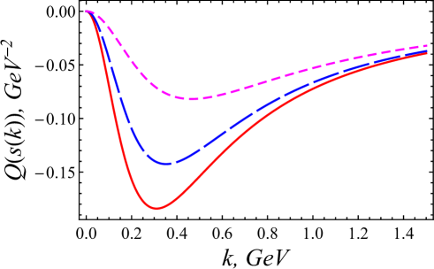
Figure 1: The $c$-number quadrupole-moment operator $Q(s(k))$ (18) as a function of $k$ for the sum of anomalous magnetic moments $a=0$ for three values of the constituent mass $M$. Solid line (red)- $M=0.22$ GeV, dashed line (blue) - $M=0.25$ GeV, short-dashed line (magenta) - $M=0.33$ GeV.

Consider the $c$-number relativistic operator of the quadrupole moment (18). The function in (18) has the following properties:

$$\lim\limits_{s\to 4M^{2}}Q(s)=0\;,\quad\lim\limits_{s\to\infty}Q(s)=0\;.$$ (21)

In Fig.1 the dependence of the function $Q(s(k))$ on the momentum variable $k$ for different constituent masses and the zero value of the sum of the anomalous magnetic moments of constituents $a=0$ is shown. The first of the equations (21) means that the contribution of the small relative momenta to the quadrupole moment is suppressed. This means that the large-distance contribution to the relativistic quadrupole moment is small. This contrasts fundamentally with the nonrelativistic case (see, e.g., BrJ76 ) when the nonrelativistic quadrupole moment is defined by the wave function at large distances. We will refer to the relativistic wave functions that give a large value of the probability for constituents to be found at large relative distances as to models with weak coupling. The corresponding relativistic quadrupole moment (17) is small. The deuteron presents an example of this type of coupling.

On the contrary, we refer to the models with the wave functions concentrated at small distances as to models with strong coupling of the constituents. In such models the relativistic quadrupole-moment values are larger.

In what follows we consider systems with weak coupling using the wave function (20) normalized to unity. The systems with the most strong coupling are realized in the model with the square-law confinement. This model with the harmonic oscillator potential is largely used in composite quark models (see, e.g., BiS14 ). The corresponding wave function in the representation (2) with quantum numbers $l=0\,,S=1$ is of the form:

$$u(k)=2\sqrt{\frac{1}{\sqrt{\pi}b^{3}}}\exp{\left(-\frac{k^{2}}{2b^{2}}\right)}\;,$$ (22)

where the parameter $b$ determines the confinement scale. We use also the model with intermediate coupling (19), that is close (see Sec. III) to the model with the linear confinement Tez91 .

It follows from the conditions (21) (see also Fig.1) that the function $Q(s(k))$ has an extremum. So, one can see that the quadrupole moment (17) is defined by the value of the overlap integral of the square of the wave function and the function (18). The largest absolute value of the quadrupole moment is to be expected in the models with the largest overlaps. In the strong-coupling model the position of the maximum of the square of the wave function (22) is defined by the parameter $b$. There exists a value $b$ that gives the maximum overlap and, so, the maximum value of the quadrupole moment. Our numerical calculations confirm this statement.

The Fig.1 demonstrates also that the absolute value of the quadrupole-moment operator decreases appreciably with increasing mass of the constituents. Consequently the absolute value of the quadrupole moment decreases and will go to zero in the limit of large masses of the constituents. This is in accordance with the fact that the quadrupole moment in the systems under consideration is a relativistic effect and disappears in the nonrelativistic limit.

Let us discuss now the dependence of the quadrupole moment on the sum of anomalous magnetic moments $a$ and dislocate the important region of this variable for study. For the deuteron, $a$ is known from the experiment with great accuracy (see Sec.III). For a quark-antiquark system, $a$ cannot be measured. However, the model independent constraints for the anomalous magnetic moments of $u$- and $d$- quarks were obtained in the paper Ger96 :

$$\frac{e_{u}+\kappa_{u}}{e_{d}+\kappa_{d}}=-1.77\;,$$ (23)

where $e_{u,d}$ are the charges of $u$- and $d$-quarks and $\kappa_{u,d}$ are their anomalous magnetic moments (in quark magnetons).

Using the equation (23) and our definition $\kappa_{u}+\kappa_{\bar{d}}=\kappa_{u}-\kappa_{d}=a$ it is easy to obtain the values of anomalous magnetic moments of the quark and the antiquark as functions of the parameter $a$. This dependence is shown in Fig.2.

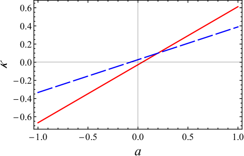
Figure 2: Anomalous magnetic moments of the $u$- and $\bar{d}$-quarks in quark magnetons as functions of the sum of anomalous magnetic moments $a$ corresponding to (23) Ger96 . Solid line (red) - $\kappa_{u}$, dashed line (blue) - $\kappa_{\bar{d}}$.

For the point-like quarks ($\kappa_{u}=\kappa_{\bar{d}}=0$), the ratio of the magnetic moments of $u$- and $d$- quarks is exactly $-2$ that is not far of (23). The deviation of (23) from this value owing to the anomalous magnetic moments is approximately 12% and can be considered as a correction. So, it is natural to consider the anomalous magnetic moments as corrections to the point-like quark magnetic moments, too. This allows one to consider in what follows the range of the values of the parameter $a$ from $-0.25$ to 0.25. Fig.2 demonstrates that this interval gives the values of anomalous magnetic moments of the quarks that are realistic from the point of view of the ratio (23). Note that the sum of anomalous magnetic moments of proton and neutron lays in this interval.

The masses of the constituent $u$- and $d$-quarks are the parameters of the composite quark model and in the current literature their values are always greater than 0.1 GeV. We choose the interval for the masses of constituents to extent from 0.1 GeV up to 1.0 GeV. The masses of the constituents in the $\rho$ meson and the deuteron enter this interval.

V Constraints on the quadrupole moment of spin one composite system in the $S$-state of relative motion

Let us derive some bounds on possible values of the quadrupole moment of two-particle systems with the total spin one in the $S$-state of the relative motion. We consider the class of the interaction models with the strongest coupling realized for the model with square-law confinement (22).

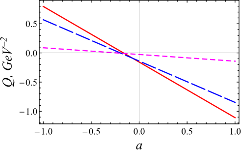
Figure 3: The quadrupole moment of composite system as a function of the sum of anomalous magnetic moments of the constituents $a$ for different model interactions at $M=0.22$ GeV. Solid(red) line - the harmonic oscillator wave function (22) with $b=0.35$ GeV KrT01 , dashed line (blue) - the power-law wave function (19), $b=0.385$ GeV KrP18 , short-dashed line (magenta) - weak coupling model (20) KrT07 .

We show that in the framework of our approach, adding physical reasoning connected with the structure of our relativistic operator of the quadrupole moment, it occurs to be possible to obtain some constraints for the values of the quadrupole moment of the composite systems with quantum numbers indicated above. As our approach have demonstrated its effectiveness for relativistic theory of very different two-particle composite systems KrT07 ; KrT01 ; KrT98 ; KrT09prc ; TrT13 ; KrP16 ; KrP18 ; KrN13 , it is plausible to expect that our constraints are of a rather general character.

The quadrupole moment of the system (17) is a function (see (18)) of three variables $Q=Q(M,b,a)$ in the case of wave functions (19) and (22). In the weak coupling model (20) there is no parameter $b$. Let us consider first the dependence of the quadrupole moment on the sum of anomalous magnetic moments $a$ of the constituents. As can be seen from (17) the quadrupole moment is a linear decreasing function of $a$ for all models of interaction. It is plotted in Fig.3 for the models (19), (20), (22) with $M=0.22$ GeV. For the model (22) we use $b=0.35$ GeV as in pion calculations KrT01 , for the model (19) we put $b=0.385$ GeV used in the unified $\pi\&\rho$ model KrP16 ; KrP18 . The weak-coupling wave function (20) was normalized to unity. Fig.3 is in accordance with the statement of Sec.IV that the largest absolute value of the quadrupole moment for the same parameters $M$ and $a$ is achieved for the model (22).

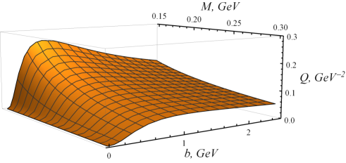
Figure 4: The quadrupole moment $Q(M,b,-a_{m})$ (17) in the region $a\leq a_{0},\;Q\geq 0$ (24) as a function of the constituent mass $M$ and the parameter of the wave function $b$ in the model of harmonic oscillator (22). $a_{0}$ is the value of the parameter $a$ for $Q=0$. The sum of the anomalous magnetic moments $a_{m}=0.25$.

Note that a value $a=a_{0}$ for which the quadrupole moment is zero exists in all models of interaction and for all values of other parameters. This is due to a compensation mechanism that suppresses the relativistic quadrupole moment in a system with the quantum numbers $S=1,\;l=0$. This mechanism is caused by the existence of a structure of constituents, namely, of the anomalous magnetic moments. The actual position of the zero value of the quadrupole moment depends weakly on $M$ and on the choice of the model.

First, let us consider the range of parameters that gives the nonnegative value of the quadrupole moment: $Q\geq$0. Takig into account the fact that $Q$ decreases linearly with $a$ in all cases we obtain that the upper bound in this domain is defined by our choice of the interval for the parameter $a$:

$$Q(M,b,a)\;\leq Q(M,b,-a_{m})\;,$$ (24)

where $-a_{m}$ is the minimal admissible value. The role that plays this parameter explains the detailed discussion in Sec.IV where we have supposed $-a_{m}=-0.25$.

Let us consider the dependence of the function $Q(M,b,-a_{m})$ on the parameters $M$ and $b$. In Sec. II analysing the structure of the operator of the quadrupole moment (18) we concluded that the quadrupole moment (17) has a maximum at some value of the parameter $b$ in (22), (19). In fact Fig.4 presenting the quadrupole moment (17) as a function of parameters $M$ and $b$ in the model (22) shows that at any fixed constituent mass $M$ the quadrupole moment has a maximum at some $b=b_{max}(M)$. So, the upper bound for the values of the quadrupole moment is a function of $M$: $Q(M,b_{max}(M),-a_{m})$. The value $b_{max}(M)$ can be obtained using the maximum condition for (17) for fixed value of the mass $M$ and $a=-a_{m}$;

$$0\leq Q(M,b,a)\leq Q(M,b_{max}(M),-a_{m})\;.$$ (25)

In Sec. IV we suggested, using qualitative reasonings, that the largest value of the quadrupole moment is reached in the strong coupling model (22). The direct numerical calculation confirms this fact and shows that for arbitrary constituent mass the following chain of the inequalities is valid:

$$0\leq Q(M,b,a)\leq Q(M,b_{max}(M),-a_{m})\leq$$

$$\leq Q_{HO}(M,b_{max}(M),-a_{m})\;,$$ (26)

where $Q_{HO}(M,b_{max}(M),-a_{m})$ is the maximal value of the quadrupole moment in the model (22) at a fixed constituent mass..

In fact the function of mass $Q_{HO}(M,b_{max}(M),-a_{m})$ gives the upper value of the quadrupole moment in our class of interaction models. In this class the model with the square-law confinement (22) presents the strongest coupling. The quadrupole moment $Q_{PL}(M,b_{max}(M),-a_{m})$ in the model with confinement close to the linear one (19) (see, e.g., KrT01 ) also achieves a maximum at some value of the model parameter $b$, the maximum value being smaller than in the model with quadratic confinement. At the same mass the value of maximum of $Q_{MT}(M,-a_{m})$ for the weak coupling model normalized function (20) is even smaller. The direct calculation for $M=0.22\,\hbox{GeV}$ gives:

$$Q_{MT}(M,-a_{m})\,<\,Q_{PL}(M,b_{max}(M),-a_{m})\,<\,$$

$$<\,Q_{HO}(M,b_{max}(M),-a_{m})\;,$$

or actually:

$$0.002\,\hbox{GeV}^{-2}\,<\,0.118\,\hbox{GeV}^{-2}\,<\,$$

$$<\,0.120\,\hbox{GeV}^{-2}\;.$$ (27)

The difference between the maxima for the models (19) and (22) is small but the inequality (26) is valid. The relations similar to (27) exist for all values of the constituent mass from a chosen interval, the difference between maxima growing with mass increasing.

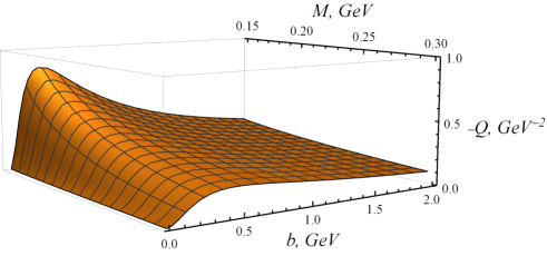
Figure 5: The opposite in sign value of the quadrupole moment -$Q(M,b,a_{m})$ (17) for $a\geq a_{0},\;Q\leq 0$ (28) as a function of the constituent mass and of the parameter $b$ of the wave function in the harmonic oscillator model (22). The sum of anomalous magnetic moments $a_{m}=0.25$.

Consider now the region where $Q\leq 0$ (see Fig.3). The linear decreasing of the quadrupole moment with increasing $a$ means that in all interaction models, the lower bound of $Q$ is given by the largest value of $a$:

$$Q(M,b,a_{m})\;\leq\;Q(M,b,a)\;\leq 0\;,$$ (28)

where $a_{m}=0.25$.

In Fig.5 the dependence of -$Q(M,b,a_{m})$ on the parameters $M$ and $b$ for the model (22) is shown. One can see that for an arbitrary fixed constituent mass, the function $Q(M,b,-a_{m})$ has a minimum at $b=b_{min}(M)$. The lower bound of the quadrupole moment is now a function of the mass $M$: $Q(M,b_{min}(M),a_{m})$.

Using reasoning and calculations analogous to those used when deriving (26), we estimate the lower boundary of the quadrupole moment:

$$Q_{HO}(M,b_{min}(M),a_{m})\leq Q(M,b_{min}(M),a_{m})\leq$$

$$\leq Q(M,b,a)\leq 0\;.$$ (29)

Here $b_{min}$ is the point of the minimal value of the quadrupole moment in the models (19) and (22) at a fixed value of the constituent mass, $Q_{HO}(M,b_{min}(M),a_{m})$ is the minimal value of the quadrupole moment in the model (22) at a fixed mass.

We can write the inequalities analogous to (27):

$$Q_{MT}(M,a_{m})\,>\,Q_{PL}(M,b_{min}(M),a_{m})\,>\,$$

$$>\,Q_{HO}(M,b_{min}(M),a_{m})\;,$$

$$-0.055\,\hbox{GeV}^{-2}\,>-0.384\,\hbox{GeV}^{-2}\,>\,$$

$$>\,-0.395\,\hbox{GeV}^{-2}\;.$$ (30)

The upper ($Q_{HO}(M,b_{max}(M),-a_{m})$) and lower ($Q_{HO}(M,b_{min}(M),a_{m})$) bounds for the values of the quadrupole moment are shown in Fig.6 and Fig.7 as functions of the constituent mass for our choice $a_{m}=0.25$.

Figure 6: The upper and the lower bounds (26), (29) for possible values of the quadrupole moment as functions of the constituent mass at $a_{m}=0.25$ in quark magnetons (24).

Figure 7: The same as in Fig.6 for other region of constituent masses.

So, for all interaction models considered in the paper, for arbitrary masses of constituents and for arbitrary sum of anomalous magnetic moment from the interval $[-0.25;0.25]$, the quadrupole moment of the two-particle system is between the curves shown in Fig.6 and Fig.7. As far as we know, it is for the first time that this kind of constraints is proposed and as such it may be ameliorated in a number of directions. The constraints are obtained in the framework of only one approach. However the advantages of our approach described above enable us to believe in the validity of the constraints. The set of the interaction models is rather limited, but we consider the interactions that are the most popular in calculations of two-particle composite systems. The choosen interval for the parameter $a$ plays a very important role and the width of the band of possible values of the quadrupole moment can be diminished efficiently for a smaller value of $a_{m}$. The detailed discussion of the choice of its value was given above. The mass interval considered is reasonably wide.

We compare some of results of different authors on the $\rho$-meson quadrupole moment with our bounds. There are some values that satisfy our constraints (see, for example, MeS02 ; BiS14 ; CaD98 ) and some others that do not.

VI Conclusions

To summarize, we construct the relativistic operator of the quadrupole moment of two-particle composite spin one system with zero angular moment using our version of RQM. We adopt the modified instant form RQM that we used previously. The derived quadrupole-moment operator in the basis with the separated motion of the center-of-mass is a $c$-number function.

Then this operator is used to calculate, with no fitting parameters, the values of the quadrupole moments of the $\rho$ meson ($Q_{\rho}=-0.158\pm 0.04$ GeV^-2) and of the $S$-wave deuteron ($Q_{d}=-1.4\cdot 10^{-4}$ GeV^-2). The quadrupole moment of the $\rho$ meson is obtained in the framework of the unified $\pi$&$\rho$ model developed by the authors in the recent papers. The quadrupole moment of the $S$-wave deuteron is calculated using the wave function obtained by the authors in a potentialless formulation of the inverse scattering problem; this function has given good results for the polarization $ed$-scattering data and for the quadrupole form factor of deuteron.

The study of the properties of the obtained quadrupole-moment operator permits to formulate, for the first time, the problem of the upper and lower bounds for possible values of the quadrupole moment of a two-particle system with indicated quantum numbers for a large range, from $0.1$ GeV to $1$ GeV, of constituent masses, and to partially solve it. The constraints are obtained in the class of interaction models for constituents with the most strong coupling realized by the square-law confinement. It is shown that our limitations depend essentially on the sum of the anomalous magnetic moments of the constituents.

Appendix

The quadrupole $g_{0Q}$ form factor for free two–particle system is:

$$g_{0Q}(s,Q^{2},s^{\prime})=\frac{1}{2}\,R(s,Q^{2},s^{\prime})\,Q^{2}$$

$$\times\left\{(s+s^{\prime}+Q^{2})(G^{1}_{E}(Q^{2})+G^{2}_{E}(Q^{2}))\right.$$

$$\times\left[\cos(\omega_{1}-\omega_{2})-\cos(\omega_{1}+\omega_{2})\right]$$

$$-\frac{1}{M}\xi(s,Q^{2},s^{\prime})(G^{1}_{M}(Q^{2})+G^{2}_{M}(Q^{2}))$$

$$\times\left.\left[\sin(\omega_{1}-\omega_{2})+\sin(\omega_{1}+\omega_{2})\right]\right\};$$

Here

$$R(s,Q^{2},s^{\prime})=\frac{(s+s^{\prime}+Q^{2})}{2\sqrt{(s-4M^{2})(s^{\prime}-4M^{2})}}\,$$

$$\times\frac{\vartheta(s,Q^{2},s^{\prime})}{{[\lambda(s,-Q^{2},s^{\prime})]}^{3/2}}\frac{1}{\sqrt{1+Q^{2}/4M^{2}}}\;,$$

$$\xi(s,Q^{2},s^{\prime})=\sqrt{ss^{\prime}Q^{2}-M^{2}\lambda(s,-Q^{2},s^{\prime})}\;,$$

$\omega_{1}$ and $\omega_{2}$ are the Wigner rotation parameters:

$$\omega_{1}=\arctan\frac{\xi(s,Q^{2},s^{\prime})}{M\left[(\sqrt{s}+\sqrt{s^{\prime}})^{2}+Q^{2}\right]+\sqrt{ss^{\prime}}(\sqrt{s}+\sqrt{s^{\prime}})}\;,$$

$$\omega_{2}=\arctan\frac{\alpha(s,s^{\prime})\xi(s,Q^{2},s^{\prime})}{M(s+s^{\prime}+Q^{2})\alpha(s,s^{\prime})+\sqrt{ss^{\prime}}(4M^{2}+Q^{2})}\;,$$

$\alpha(s,s^{\prime})=2M+\sqrt{s}+\sqrt{s^{\prime}}$, $\vartheta(s,Q^{2},s^{\prime})=\theta(s^{\prime}-s_{1})-\theta(s^{\prime}-s_{2})$, $\theta$ is the step–function.

$$s_{1,2}=2M^{2}+\frac{1}{2M^{2}}(2M^{2}+Q^{2})(s-2M^{2})$$

$$\mp\frac{1}{2M^{2}}\sqrt{Q^{2}(Q^{2}+4M^{2})s(s-4M^{2})}\;.$$

$\lambda(a,b,c)=a^{2}+b^{2}c^{2}-2(ab+ac+bc),$ $M$ – the mass of a constituent, for example the $u$ or $\bar{d}$ quark or a nucleon. The functions $s_{1,2}(s,Q^{2})$ give the kinematically available region in the plane $(s,s^{\prime})$. $G^{1,2}_{E,M}(Q^{2})$– charge and magnetic Sachs form factors of constituents, respectively.

The ansatz for the analytic versions of the $p$-space $S$ deuteron wave function, denoted by $u(k)$, is given by (20). In (20)

$$m_{j}=\alpha+m_{0}\,(j-1)\;,$$

the coefficients $C_{j}$, the maximal value of the index $j$ and $m_{0}=0.9$ fm^-1 are defined by the condition of the best fit. One has $\alpha=\sqrt{M\,\varepsilon_{d}}\;$, $\;M=0.93891870$ GeV is average nucleon mass, $\varepsilon_{d}=2.224996\cdot 10^{-3}$ GeV is the binding energy of the deuteron in the model KrT07 .

Table 1: Coefficients for the parametrized $S$ deuteron wave function calculated within a dispersion approach. The last $C_{j}$ is to be computed from eq. (A3) ($n_{u}$=16).

$j$	$C_{j}({\rm fm}^{-1/2})$	$j$	$C_{j}({\rm fm}^{-1/2})$
1	0.87872995​+​00	9	0.59953379​+​07
2	-0.50381047​+​00	10	-0.11282284​+​08
3	0.28787196​+​02	11	0.15181681​+​08
4	-0.82301294​+​03	12	-0.14519973​+​08
5	0.12062383​+​05	13	0.96491938​+​07
6	-0.10574260​+​06	14	-0.42403857​+​07
7	0.59534957​+​06	15	0.11092702​+​07
8	-0.22627706​+​07	16	eq. (A3)

$$\sum\limits_{j=1}^{n_{u}}{C_{j}}=0\;.$$

References

- (1) A. S. Bagdasaryan, S. V. Esaibegian, and N. L. Ter-Isaakian, Form factors of meson and resonances at small and intermediate momentum transfers in the relativistic quark models, Yad. Fiz. 42, 440 (1985) [Sov. J. Nucl. Phys. 42, 278 (1985)].
- (2) F. Cardarelli, I.L. Grach, I.M. Narodetskii, G. Salmé, S. Simula, Electromagnetic form factors of the meson in a light-front constituent quark model, Phys. Lett. B 349, 393 (1995), [arXiv:hep-ph/9502360].
- (3) P. L. Chung, F. Coester, B. D. Keister, and W. N. Polyzou, Hamiltonian light-front dynamics of elastic electron deuteron scattering, Phys. Rev. C 37, 2000 (1988).
- (4) J. P. B. C. de Melo and T. Frederico, Covariant and light-front approaches to the meson electromagnetic form factors, Phys. Rev. C 55, 2043 (1997), [arXiv:nucl-th/9706032].
- (5) J. Carbonell, B. Desplanques, V.A. Karmanov, and J.P. Mathiot, Explicitly covariant light-front dynamics and relativistic few-body systems, Phys. Rep. 300, 215 (1998).
- (6) B.L.G. Bakker, Ho-Meoyng Choi and Chueng-Ryong Ji, The vector meson form-factor analysis in light front dynamics, Phys. Rev. D 65, 116001 (2002), [arXiv:hep-ph/0202217].
- (7) W. Jaus, Consistent treatment of spin-1 mesons in light-front quark model, Phys. Rev. D 67, 094010 (2003), [arXiv:hep-ph/0212098].
- (8) H.-M. Choi, C.-R. Ji, Electromagnetic structure of the meson in the light-front quark model, Phys.Rev.D 70, 053015 (2004), [arXiv:hep-ph/0402114].
- (9) Jun He, B. Juliá-Díaz, and Y.-B. Dong, Electromagnetic form factors of pion and meson in the three forms of relativistic kinematics, Phys. Lett. B 602, 212 (2004), [arXiv:hep-ph/0407043].
- (10) E.P. Biernat and W. Schweiger, Electromagnetic meson form factors in point-form relativistic quantum mechanics, Phys. Rev. C 89, 055205 (2014), [arXiv:1404.2440[hep-ph]].
- (11) C.S. Mello, A.N. da Silva, J.P.B.C. de Melo, T. Frederico, ”Light-Front Spin-1 Model: parameters dependence”, Few-Body Syst,56, 509 (2015).
- (12) B.-D. Sun and Y.-B. Dong, meson unpolarized generalized parton distrbutions with a light-front constituent quark model, Phys. Rev. D 96 no.3, 036014 (2017), [arXiv:1707.03972 v2 [hep-ph]].
- (13) E.T. Hawes and M. A. Pichowsky, Electromagnetic form factors of light vector mesons, Phys. Rev. C 59 , 1743 (1999), [arXiv:nucl-th/9806025].
- (14) M.S. Bhagwat and P. Maris, Vector meson form factors and their quark-mass dependence, Phys. Rev. C 77, 025203 (2008), [arXiv:nucl-th/0612069].
- (15) H.L.L. Roberts, A. Bashir, L.X. Gutierrez-Guerrero, C.D. Roberts, and D.J. Wilson, - and mesons, and their diquark partners, from a contact interaction, Phys. Rev. C 83, 065206 (2011), [arXiv:1102.4376 [nucl-th]].
- (16) M. Pitschmann, C-Y. Seng, M. J. Ramsey-Musolf, C. D. Roberts, and D.J. Wilson, Electrc dipole moment of the meson, Phys. Rev. C 87, 015205 (2013), [arXiv:1209.4352[nucl-th]].
- (17) M. E. Carrillo-Serrano, W. Bentz, I. C. Cloët, and A. W. Thomas, Rho meson form factors in confining Nambu–Jona-Lasino model, Phys. Rev. C 92, 015212 (2015), [arXiv:1504.08119 [nucl-th]].
- (18) Y.-L. Luan, X.-L. Chen, and W.-Z. Deng, Chin. Phys., Meson Electro-Magnetic Form Factors in an Extended Nambu-Jona-Lasinio model including Heavy Quark Flavors, C39 no 11, 113103 (2015), [arXiv:1504.03799 [hep-ph]].
- (19) A. Samsonov, Magnetic moment of the meson in QCD sum rules: - corrections, JHEP 12, 061 (2003), [arXiv:hep-ph/0308065].
- (20) T.M. Aliev, A. Özpineci, M. Savci, Magnetic and quadrupole moments of light spin-1 mesons in light cone QCD sum rules, Phys. Lett. B 678, 470 (2009), [arXiv:0902.4627[hep-ph]].
- (21) D. Melikhov and S. Simula, Electromagnetic form factors in the light–front formalism and the Feynman triangle diagram: Spin-0 and spin-1 two–fermion systems, Phys. Rev. D 65, 094043 (2002), [arXiv:hep-ph/0112044].
- (22) W. Andersen and W. Wilcox, Lattice charge overlap. I. Elastic limit of and mesons, Ann. of Phys., 255, 34 (1997), [arXiv:hep-lat/9502015].
- (23) J.N. Hedditch, W. Kamleh, B.G. Lasscock, D.B. Leinweber, A.G. Williams, and J.M. Zanotti, Pseudoscalar and vector meson form factors from lattice QCD, Phys.Rev.D 75,094504 (2007), [arXiv:hep-lat/0703014].
- (24) B. Owen, W. Kamel, D. Leinweber, B. Menadue, S. Mahbub, Light meson form factors at near physical masses, Phys. Rev. D 91, 074503 (2015), [arXiv:1505.02876[hep-lat]]..
- (25) E.V. Lushevskaya, O. E. Solovjeva, and O. V. Teryaev, Determination of the properties of vector mesons in external magnetic field by quenched SU(3) lattice QCD, JHEP 09 (2017) 142, [arXiv:1608.03472 [hep-lat]].
- (26) Yu.V. Novozhilov, Introduction to Elementary Particle Theory (Oxford University Press, New York, 1975).
- (27) S.J. Brodsky and J.R. Hiller, Universal properties of the electromagnetic interactions of spin-one systems, Phys. Rev. D 46, 2141 (1992).
- (28) M. Garçon and J.W.van Orden, The deuteron: structure and form factors, Adv.Nucl.Phys. 26 (2001) 293.
- (29) R. Gilman and F. Gross, Electromagnetic structure of the deuteron, J. Phys. G 28 (2002) R37.
- (30) P.A.M. Dirac, Forms of relativistic dynamics, Rev. Mod. Phys. 21 (1949) 392.
- (31) H. Leutwyler and J. Stern, Relativistic dynamics on null plane, Ann. Phys. 112 (1978) 94.
- (32) B.D. Keister and W.N. Polyzou, Relativistic Hamiltonian dynamics in nuclear and particle physics, Adv. Nucl. Phys. 20 (1991) 225.
- (33) F. Coester, Null–plane dynamics of particles and fields, Prog.Part.Nucl.Phys. 29 (1992) V.29. 1.
- (34) A.F. Krutov and V.E. Troitsky, Instant form of Poincaré-invariant quantum mechanics and description of the structure of composite systems, Phys. Part. Nucl. 40 (2009) 136.
- (35) A.F. Krutov and V.E. Troitsky, Deuteron tensor polarization component as a crucial test for deuteron wave functions, Phys.Rev. C 75 (2007) 014001.
- (36) A.F. Krutov and V.E. Troitsky, On a possible estimation of the constituent quark parameters from Jefferson Lab experiments on pion form factor, Eur. Phys. J. C 20 (2001) 71 [hep-ph/9811318].
- (37) A.F. Krutov and V.E. Troitsky, Asymptotic estimates of the pion charge form-factor, Theor. Math. Phys. 116 (1998) 907 [Teor. Mat. Fiz. 116 (1998) 215].
- (38) A.F. Krutov, V.E. Troitsky and N.A. Tsirova, Nonperturbative relativistic approach to pion form factor versus JLab experiments, Phys. Rev. C 80 (2009) 055210 [arXiv:0910.3604 [nucl-th]].
- (39) S.V. Troitsky and V.E. Troitsky, Transition from a relativistic constituent-quark model to the quantum-chromodynamical asymptotics: a quantitative description of the pion electromagnetic form factor at intermediate values of the momentum transfer, Phys. Rev. D 88 (2013) 093005 [arXiv:1310.1770 [hep-ph]].
- (40) A.F. Krutov, R.G. Polezhaev and V.E. Troitsky, The radius of the meson determined from its decay constant, Phys. Rev. D 93 (2016) 036007 [arXiv:1602.00907 [hep-ph]].
- (41) A.F.Krutov, R.G.Polezhaev, and V.E.Troitsky, Magnetic moment of the meson in instant-form relativistic quantum mechanics, Phys.Rev. D 97 (2018) 033007.
- (42) A.F.Krutov, S.V.Troitsky, and V.E.Troitsky, The K-meson form factor and charge radius: linking low-energy data to future Jefferson Laboratory measurements, Eur. Phys. J. C 77 (2017) 464.
- (43) J. Volmer et al. (Jefferson Lab Collaboration), Measurement of Charged Pion Electromagnetic Form-Factor, Phys. Rev. Lett. 86 (2001) 1713 [nucl-ex/0010009].
- (44) T. Horn et al. (Jefferson Lab Collaboration), Determination of Charged Pion Form Factor at and (GeV/c)2, Phys. Rev. Lett. 97 (2006) 192001 [nucl-ex/0607005].
- (45) V. Tadevosyan et al.(Jefferson Lab Collaboration), Determination of pion charge form factor for - -(GeV/c)2, Phys. Rev. C 75 (2007) 055205 [nucl-ex/0607007].
- (46) H. P. Blok et al. (Jefferson Lab Collaboration), Charged pion form factor between and 2.45 GeV2. I. Measurmente of the cross section for the reaction, Phys. Rev. C 78 (2008) 045202 [arXiv:0809.3161 [nucl-ex]].
- (47) G. M. Huber et al (Jefferson Lab Collfboration), Charged pion form factor between = 0.60 and 2.45 GeV2. II. Determination of, and results for, the pion form factor, Phys. Rev C 78, 045203 (2008) [arXiv:0809.3052 [nucl-ex]].
- (48) S.V. Troitsky and V.E. Troitsky, Constraining scenarios of the soft/hard transition for pion electromagnetic form factor of 12 GeV Jefferson Lab experiments and of the electron-ion collaider, Phys. Rev. D 91, 033008 (2015) [arXiv:1501.02712[hep-ph]].
- (49) A.F. Krutov, M.A. Nefedov, V.E. Troitsky, Analytic continuation of the pion form factor from the spacelike to the timelike domain, Theor. Math. Phys. 2013, 174 (2013) 331 [Teor. Mat. Fiz. 174 (2013) 383].
- (50) A.F. Krutov and V.E. Troitsky, Parametrization of the deuteron wave function obtained within a dispersion approach, Phys.Rev. C 76 (2007) 017001.
- (51) V. M. Muzafarov and V. E. Troitsky, Electromagnetic deuteron structure, Yad. Fiz. 33, 1461 (1981) [Sov. J. Nucl. Phys. 33, 783 (1981)].
- (52) V. E. Troitsky, The potentialless approach to the inverse scttering problem, in Proceedings of Quantum Inversion Theory and Applications, Germany, 1993, edited by H. V. von Geramb (Springer, Berlin, 1994), p. 50; Lecture Notes in Physics 427.
- (53) B. Bakamjian, L.H. Thomas, Relativistic particle dynamics.II, Phys.Rev. 92 (1953) 1300.
- (54) A.A. Cheshkov and Yu.M. Shirokov, Invariant parametrization of local operators, Zh. Eksp. Teor. Fiz. 44 (1963) 1982 [Sov. Phys. JETP 17 (1963) 1333].
- (55) A.F. Krutov and V.E. Troitsky, Relativistic instant form approach to the structure of two-body composite systems. Nonzero spin, Phys. Rev. C 68 (2003) 018501 [hep-ph/0210046].
- (56) R.G. Arnold, C.E. Carlson, F. Gross, Elastic electron-deuteron scattering at high energy, Phys. Rev. C 21 (1980) 1426.
- (57) C. Patrignani et al. (Particle Data Group), Chin. Phys. C 40 (2016) 100001.
- (58) G.E. Brown and A.D. Jackson, Introduction to Elementary Particle Theory (American Elsevier Publishing Company, New York, 1976).
- (59) H. Tezuka, Analytical solution of the Schrödinger equation with linear confinement potential, J.Phys.A. Math.Gen. 24 (1991) 5267.
- (60) S.B. Gerasimov, Electroweak moments of baryons and hidden strangeness of the nucleon, Chin. J. Phys. 34 (1996) 848 [hep-ph/9906386].