An entropy stable high-order discontinuous Galerkin method
for
cross-diffusion gradient flow systems
Zheng Sun111Department of Mathematics, The Ohio State University, Columbus, OH 43210, USA. E-mail: sun.2516@osu.edu., José A. Carrillo222Department of Mathematics, Imperial College London, London SW7 2AZ, UK. E-mail: carrillo@imperial.ac.uk. and Chi-Wang Shu333Division of Applied Mathematics, Brown University, Providence, RI 02912, USA. E-mail: shu@dam.brown.edu.
Abstract
As an extension of our previous work in [41], we develop a discontinuous Galerkin method for solving cross-diffusion systems with a formal gradient flow structure. These systems are associated with non-increasing entropy functionals. For a class of problems, the positivity (non-negativity) of solutions is also expected, which is implied by the physical model and is crucial to the entropy structure. The semi-discrete numerical scheme we propose is entropy stable. Furthermore, the scheme is also compatible with the positivity-preserving procedure in [42] in many scenarios. Hence the resulting fully discrete scheme is able to produce non-negative solutions. The method can be applied to both one-dimensional problems and two-dimensional problems on Cartesian meshes. Numerical examples are given to examine the performance of the method.
Keywords: discontinuous Galerkin method, entropy stability, positivity-preserving, cross-diffusion system, gradient flow
1 Introduction
Cross-diffusion systems are widely used to model multi-species interactions in various applications, such as population dynamics in biological systems [39], chemotactic cell migration [32], spread of surfactant on the membrane [26], interacting particle systems with volume exclusion [5, 2], and pedestrian dynamics [24]. In many situations, the systems are associated with neither symmetric nor positive-definite diffusion matrices, which not only complicate the mathematical analysis but also hinder the development of numerical methods. Recently, progress has been made in analyzing a class of cross-diffusion systems having the structure of a gradient flow associated with a dissipative entropy (or free energy) functional, see [28, 30, 31] and references therein. We will exploit this gradient flow structure to develop a high-order stable discontinuous Galerkin (DG) method for these cross-diffusion systems.
Let be a bounded domain in . We are interested in solving the following initial value problem of the cross-diffusion system.
| (1.1) |
Here and is a vector-valued function as well as with being a scalar-valued twice differentiable convex function. We also assume to be an positive-semidefinite -dependent matrix, in the sense that . Note can be non-symmetric. Equation (1.1) can be written in divergence form as , with the matrix possibly neither symmetric nor positive-definite.
The system (1.1) possesses a formal gradient flow structure governed by the entropy functional
| (1.2) |
The system can be rewritten as . One can see at least for classical solutions that
| (1.3) |
with the usual notation for the matrix product of square matrices . The Liapunov functional (1.2) due to (1.3) indicates certain well-posedness of the initial value problem (1.1). However, in applications with representing non-negative physics quantities, such as species densities, mass fractions and water heights, the well-posedness usually relies heavily on the positivity of the solution. For example, with , is semi-positive definite only when is non-negative. Violating the non-negativity may result in a non-decreasing entropy in (1.3). Furthermore, in problems that a logarithm entropy is considered, the entropy may not even be well-defined when admits negative values.
The entropy structure is crucial to understand various theoretical properties of cross-diffusion systems, such as existence, regularity and long time asymptotics of weak solutions, see [28, 30, 31]. It is desirable to design numerical schemes that preserve the entropy decay in (1.3), and would also be positivity-preserving if the solution to the continuum equation is non-negative, due to the concern we have mentioned. Various efforts have been spent on numerical methods for scalar problems with a similar entropy structure, including the mixed finite element method [4], the finite volume method [3, 6], the direct DG method [33, 34], optimal mass transportation based methods [11, 27, 12, 10], the particle method [9] and the blob method [21, 7]. Some methods can also be generalized to systems, for example the Poisson-Nerst-Plack system [35] and system of interacting species with cross-diffusion [8].
In this paper, we extend the DG method in [41] for scalar gradient flows to cross-diffusion systems. The DG method is a class of finite element methods utilizing discontinuous piecewise polynomial spaces, which was originally designed for solving transport equations [38] and was then developed for nonlinear hyperbolic conservation laws [18, 17, 16, 15, 20]. The method has also been generalized for problems involving diffusion and higher order derivatives, for example, the local DG method [1, 19], the ultra-weak DG method [14] and the direct DG method [36]. The method preserves local conservation, achieves high-order accuracy, is able to handle complex geometry and features with good - adaptivity and high parallel efficiency. As an effort to incorporate these potential advantages in gradient flow simulations, in [41], we adopted the technique from [13] to combine the local DG methods with Gauss-Lobatto quadrature rule, and designed a DG method for scalar gradient flows that is entropy stable on the semi-discrete level. This method also features weak positivity with Euler forward time stepping method. Hence after applying a scaling limiter and the strong-stability-preserving Runge-Kutta (SSP-RK) time discretization [23], the fully discrete scheme produces non-negative solutions. This positivity-preserving procedure is established in [43, 42, 40].
The main idea for handling cross-diffusion systems is to formally rewrite the problem into decoupled equations and apply our previous numerical strategy in [41] for scalar gradient flows to the unknown density vector component-wise. In fact, the system (1.1) can be rewritten as
In the particular case of one dimension, we are reduced to apply our previous scheme in [41] to , for . The numerical fluxes are properly chosen to ensure the entropy decay and the weak positivity. In this approach, the boundedness of is required for to be well-defined. This assumption does hold in various applications, see examples in Section 4 and Section 5.
The rest of the paper is organized as follows. In Section 2 and Section 3, we propose our DG schemes for one-dimensional and two-dimensional gradient flow systems respectively. Each section is composed of three parts: notations, semi-discrete scheme and entropy inequality, and fully discrete scheme as well as positivity-preserving techniques for producing non-negative solutions (with central and Lax-Friedrichs fluxes). In Section 4 and Section 5, we show several numerical examples to examine the performance of the numerical schemes. Finally, concluding remarks are given in Section 6.
2 Numerical method: one-dimensional case
2.1 Notations
In this section, we consider the one-dimensional problem
| (2.1) |
For simplicity, the compact support or periodic boundary condition is assumed, while it can also be extended to the zero-flux boundary condition.
Let and be a regular partition of the domain . The length of the mesh cell is denoted by . We assume and for some fixed constant . The numerical solutions are defined in the tensor product space of discontinuous piecewise polynomials
is the space of polynomials of degree on . Functions in () can be double-valued at cell interfaces. We use () and () to represent the left and right limits of () respectively. We also introduce notations () for the averages and () for the jumps.
Let be the Gauss-Lobatto quadrature points on and be the corresponding weights associated with the normalized interval . We introduce the following notations for the quadrature rule.
Here is a component-wise interpolation operator. Namely, , and the -th component of is the -th order interpolation polynomial of at Gauss-Lobatto points. We also define .
2.2 Semi-discrete scheme and entropy stability
We firstly rewrite (2.1) into a first-order system.
On each mesh cell , we multiply with a test function and integrate by parts to get
The numerical scheme is obtain by taking trial and test functions from the finite element space, replacing cell interface values with numerical fluxes and applying the quadrature rule. More precisely, we seek such that for all ,
| (2.2a) | ||||
| (2.2b) | ||||
Here , , and , , are defined similarly. We have the following choices for and .
(1) Central and Lax-Friedrichs fluxes:
| (2.3) |
where
and is the norm on .
(2) Alternating fluxes:
| (2.4) |
Remark 2.1.
We define the discrete entropy
| (2.5) |
As is stated in Theorem 2.1, the numerical scheme has a decaying entropy as that for the continuum system.
Theorem 2.1 (Entropy inequality).
Let and be obtained from (2.2), (2.3) and (2.4). is the associated discrete entropy defined in (2.5). Then
(1) for central and Lax-Friedrichs fluxes,
(2) for alternating fluxes,
Proof.
A direct computation yields
Then, with in (2.2a), we have
Here we have used the fact that is a polynomial of degree and that the Gauss-Lobatto quadrature rule is exact. Then again with integrating by parts and the exactness of the quadrature, one can get
where in the last identity we used the scheme (2.2b) with . After summing over the index and using the periodicity, we obtain
The proof is completed by substituting numerical fluxes in (2.3) and (2.4). Note that
due to the convexity of . Here lies in the line segment between and . ∎
Remark 2.2.
Both choices of numerical fluxes are entropy stable, while they have different advantages and disadvantages. For central and Lax-Friedrichs fluxes defined in (2.3), they preserve positive cell averages as time steps are small. Hence the positivity-preserving limiter can be applied for producing non-negative solutions. Details are given in the next section. However, they are limited to problems satisfying with being the matrix norm, so that can be well-defined. Furthermore, for odd-order polynomials, one would observe a reduced order of accuracy with this particular choice of . See accuracy tests in Section 4 and Section 5. Alternating fluxes do not have such order reduction and restriction on , while it may fail to preserve non-negative cell averages after one Euler forward step.
Remark 2.3.
Due to the possible degeneracy of the problem, in general it is not easy to extend the entropy decay property to fully discrete explicit schemes. When is uniformly positive-definite and is strongly convex, a fully discrete entropy inequality can be derived. We postpone to Appendix A a proof of such result, where we consider the Euler forward time discretization with central and Lax-Friedrichs fluxes.
2.3 Fully discrete scheme and preservation of positivity
2.3.1 Euler forward time stepping
When central and Lax-Friedrichs fluxes are used, one can adopt the methodology introduced by Zhang et al. in [43, 42, 40] to enforce positivity of the solution.
It can be shown, when the solution achieves non-negative values at the current
time level, with fluxes defined in
(2.3) and
a sufficiently small time step, the Euler forward time discretization will produce
a solution with non-negative cell averages at the next time level. This is
referred to as the weak positivity.
Then we can apply a scaling limiter, squashing the solution
polynomials towards
cell averages to avoid inadmissible negative values.
It is shown in [42] that the limiter preserves the high-order spatial
accuracy.
Theorem 2.2.
1. Suppose for all and . Take
then the preliminary solution obtained through the Euler forward time stepping
has non-negative cell averages.
2. Let
Define so that
Then is non-negative. Furthermore, the interpolation polynomial maintains spatial accuracy in the sense that
where is a constant depending only on the polynomial degree .
Proof.
Remark 2.4 (Pointwise non-negativity).
The procedure stated in Theorem 2.2 only guarantees the non-negativity of the solution at all Gauss-Lobatto points. This would be enough for most scenarios, since the scheme is defined only through these points. One can also ensure pointwise non-negativity of solution polynomials on the whole interval by taking .
Remark 2.5 (Time steps).
As has been analyzed for the scalar case in Remark 2.2 in [41], we expect the time step to be for some constant . In practice, we assume a diffusion number . If a negative cell average emerges, we halve the time step and redo the computation. Theorem 2.2 guarantees that the halving procedure will end after finite loops.
Remark 2.6 (The scaling parameter).
For robustness of the algorithm, especially for dealing with log-type entropy functionals, we introduce a parameter and use instead of in our computations. In other words, if , we scale the polynomial to require it takes values not smaller than at Gauss-Lobatto points; otherwise, we set the solution to be the constant in the interval. Note as long as , the accuracy could still be maintained.
Remark 2.7 (Other bounds).
In general, it would be difficult to preserve other bounds besides positivity though this procedure. Similar difficulty has also been encountered in [40].
2.3.2 High-order time discretization
We adopt SSP-RK methods for high-order time discretizations. Since the time step will be chosen as , the first-order Euler forward time stepping would be sufficiently accurate for to achieve the second-order accuracy. For and , we apply the second-order SSP-RK method
For and , a third-order time discretization method should be used
As one can see, SSP-RK methods can be rewritten as convex combinations of Euler forward steps. Hence if the time step is chosen to be sufficiently small, and the scaling limiter is applied at each Euler forward stage, then the solution will remain non-negative after one full time step.
3 Numerical method: two-dimensional case
3.1 Notations
In this section, we generalize the previous ideas to two-dimensional systems of the form
The problem is set on a rectangular domain with the compact support or periodic boundary condition. We consider a regular Cartesian mesh on , with , , and . Let and . Then the solution is sought in the following finite element space.
is the tensor product space of and . For ,
Same notations will be used in the scalar case . Finally, for the quadrature rule, we denote by and .
3.2 Semi-discrete scheme and entropy inequality
The semi-discrete scheme is given as follows. Find , and in , such that for all , and in , we have
As that in the one-dimensional case, two choices of numerical fluxes can be used.
(1) Central and Lax-Friedrichs flux
(2) Alternating fluxes
The numerical scheme mimics a similar entropy decay behavior as the continuum equation. We define the discrete entropy
| (3.1) |
We state the following entropy decay property for the semi-discrete scheme.
Theorem 3.1.
Let , and be obtained from the semi-discrete scheme for two-dimensional problems. defined in (3.1) is the discrete entropy.
(1) Suppose central and Lax-Friedrichs fluxes are used, then
(2) Suppose alternating fluxes are used, then
Proof.
Following the blueprint of the one dimensional case, we get by a direct computation that
Then using the scheme, we deduce
For each fixed , each component of is a polynomial of degree with respect to . Analogously, is a -th order polynomial with respect to for each fixed . Hence the Gauss-Lobatto quadrature with node is exact. We then replace the quadrature rule with the exact integral, and integrate by parts to get
Again by changing back to the quadrature rule and applying the scheme, we obtain
Since we have assumed periodicity, all cell interface terms cancel out with alternating fluxes.
For central and Lax-Friedrichs fluxes, there remain additional penalty terms.
since is positive-semidefinite and is convex as in the one dimensional case. ∎
3.3 Fully discrete scheme and preservation of positivity
One can adopt similar positivity-preserving techniques as in the one dimensional case, when central and Lax-Friedrichs fluxes are used. Again, the key step is to ensure the non-negativity of the first-order Euler forward time discretization. The positivity will be automatically preserved by the SSP-RK time discretization. For the first-order scenario, we could prove the following theorem.
Theorem 3.2.
1. Suppose for all , , and . Take
Then the preliminary solution obtained through the Euler forward time discretization has non-negative cell averages.
2. Let
Define so that
Then is non-negative. Furthermore, would maintain the spatial accuracy achieved by .
Proof.
Using the scheme we obtain
Note that the numerical fluxes can be rewritten as
Let
and
Then we have
which formally reduces to the scalar case. One can follow the proof of Theorem 3.1 in [41] to show that , if the prescribed time step restriction is satisfied. The non-negativity of can be justified using the definition of . ∎
Remark 3.1.
As before, pointwise non-negative solutions can be obtained by taking . The time step will be used for time marching. As negative cell averages emerge, we halve the time step. We will also use instead of when applying the scaling limiter. Here .
4 One-dimensional numerical tests
In this section, we apply the entropy stable DG method for solving one-dimensional problems. In Example 4.1 and Example 4.2, the accuracy of the scheme is examined. The error is measured with the discrete norm associated with the Gauss-Lobatto quadrature rule. We do not invoke the positivity-preserving limiter in either tests, to exclude order degeneracy due to the temporal order reduction. See [43, 40] for relevant numerical experiments. Then we consider systems from tumor encapsulation (Example 4.3) and surfactant spreading (Example 4.4) . In these tests, leading fronts are formed and the issue of positivity arises.
Example 4.1 (Heat equations).
Let us first consider the initial value problem with decoupled heat equations,
on with the periodic boundary condition. and are taken as our initial condition. The system is associated with the entropy . Hence and . We compute up to , with time step set as . Positivity-preserving limiter is not activated. We use the Lax-Friedrichs flux and alternating fluxes respectively for computation. As one can see from Table 4.1 and Table 4.2, optimal order of convergence is achieved with the alternating fluxes. The order of accuracy seems to be degenerated when we use central and Lax-Friedrichs fluxes with odd-order polynomials. This may related with the fact that the problem is smooth hence the jump term is too small, hence the Lax-Friedrichs flux is close to the central flux when the mesh is not well refined, which would cause order reduction. In Table 4.3, we document the error with different Lax-Friedrichs constants, with replaced by . As one can see, the optimal order is retrieved as becomes large. We also remark, choosing a larger Lax-Friedrichs constant does not affect the compatibility with positivity-preserving procedure, while it does make the time step more restrictive.
| error | order | error | order | error | order | ||
|---|---|---|---|---|---|---|---|
| 1 | 80 | 8.802E-04 | - | 4.958E-04 | - | 4.226E-04 | - |
| 160 | 3.948E-04 | 1.16 | 2.224E-04 | 1.16 | 1.899E-04 | 1.15 | |
| 320 | 1.609E-04 | 1.30 | 9.077E-05 | 1.29 | 7.821E-05 | 1.28 | |
| 640 | 5.647E-05 | 1.51 | 3.201E-05 | 1.50 | 2.806E-05 | 1.48 | |
| 2 | 80 | 7.760E-06 | - | 8.881E-06 | - | 1.456E-05 | - |
| 160 | 9.600E-07 | 3.02 | 1.113E-06 | 3.00 | 1.825E-06 | 3.00 | |
| 320 | 1.194E-07 | 3.01 | 1.395E-07 | 3.00 | 2.285E-07 | 3.00 | |
| 640 | 1.489E-08 | 3.00 | 1.745E-08 | 3.00 | 2.859E-08 | 3.00 | |
| 3 | 80 | 6.027E-07 | - | 4.185E-07 | - | 8.166E-07 | - |
| 160 | 5.914E-08 | 3.35 | 4.133E-08 | 3.34 | 8.365E-08 | 3.29 | |
| 320 | 5.003E-09 | 3.56 | 3.551E-09 | 3.54 | 7.567E-09 | 3.47 | |
| 640 | 3.702E-10 | 3.76 | 2.685E-10 | 3.73 | 6.054E-10 | 3.64 | |
| 4 | 80 | 6.210E-10 | - | 6.542E-10 | - | 2.194E-09 | - |
| 160 | 1.887E-11 | 5.04 | 2.030E-11 | 5.01 | 6.809E-11 | 5.01 | |
| 320 | 5.823E-13 | 5.02 | 6.338E-13 | 5.00 | 2.128E-12 | 5.00 | |
| 640 | 1.808E-14 | 5.01 | 1.981E-14 | 5.00 | 6.653E-14 | 5.00 |
| error | order | error | order | error | order | ||
|---|---|---|---|---|---|---|---|
| 1 | 80 | 4.027E-03 | - | 2.214E-03 | - | 1.591E-03 | - |
| 160 | 1.006E-03 | 2.00 | 5.530E-04 | 2.00 | 4.004E-04 | 1.99 | |
| 320 | 2.515E-04 | 2.00 | 1.382E-04 | 2.00 | 1.003E-04 | 2.00 | |
| 640 | 6.288E-05 | 2.00 | 3.455E-05 | 2.00 | 2.508E-05 | 2.00 | |
| 2 | 80 | 1.541E-05 | - | 1.418E-05 | - | 3.049E-05 | - |
| 160 | 1.912E-06 | 3.01 | 1.769E-06 | 3.00 | 3.736E-06 | 3.03 | |
| 320 | 2.383E-07 | 3.00 | 2.211E-07 | 3.00 | 4.624E-07 | 3.01 | |
| 640 | 2.975E-08 | 3.00 | 2.763E-08 | 3.00 | 5.752E-08 | 3.01 | |
| 3 | 80 | 1.219E-07 | - | 1.116E-07 | - | 4.006E-07 | - |
| 160 | 7.609E-09 | 4.00 | 6.966E-09 | 4.00 | 2.513E-08 | 4.00 | |
| 320 | 4.754E-10 | 4.00 | 4.353E-10 | 4.00 | 1.572E-09 | 4.00 | |
| 640 | 2.971E-11 | 4.00 | 2.720E-11 | 4.00 | 9.828E-11 | 4.00 | |
| 4 | 80 | 1.09E-09 | - | 1.08E-09 | - | 4.41E-09 | - |
| 160 | 3.401E-11 | 5.00 | 3.365E-11 | 5.00 | 1.374E-10 | 5.00 | |
| 320 | 1.062E-12 | 5.00 | 1.052E-12 | 5.00 | 4.278E-12 | 5.01 | |
| 640 | 3.319E-14 | 5.00 | 3.286E-14 | 5.00 | 1.334E-13 | 5.00 |
| error | order | error | order | error | order | ||
|---|---|---|---|---|---|---|---|
| 0 | 80 | 8.029E-07 | - | 5.549E-07 | - | 1.031E-06 | - |
| 160 | 1.007E-07 | 3.00 | 6.949E-08 | 3.00 | 1.294E-07 | 2.99 | |
| 320 | 1.259E-08 | 3.00 | 8.689E-09 | 3.00 | 1.618E-08 | 3.00 | |
| 640 | 1.575E-09 | 3.00 | 1.086E-09 | 3.00 | 2.022E-09 | 3.00 | |
| 80 | 4.721E-07 | - | 3.300E-07 | - | 6.683E-07 | - | |
| 160 | 4.003E-08 | 3.56 | 2.841E-08 | 3.54 | 6.043E-08 | 3.47 | |
| 320 | 2.952E-09 | 3.76 | 2.148E-09 | 3.73 | 4.843E-09 | 3.64 | |
| 640 | 2.028E-10 | 3.86 | 1.502E-10 | 3.84 | 3.560E-10 | 3.77 | |
| 80 | 1.572E-07 | - | 1.150E-07 | - | 2.605E-07 | - | |
| 160 | 1.053E-08 | 3.90 | 7.906E-09 | 3.86 | 1.892E-08 | 3.78 | |
| 320 | 6.830E-10 | 3.95 | 5.221E-10 | 3.92 | 1.300E-09 | 3.86 | |
| 640 | 4.356E-11 | 3.97 | 3.366E-11 | 3.96 | 8.619E-11 | 3.92 |
Example 4.2 (SKT population model).
We use the population model of Shigesada, Kawashima and Teramoto [39] for the second accuracy test. All the cross-diffusion and self-diffusion coefficients are taken as . The system is written as follows.
| (4.1a) | |||
| (4.1b) | |||
(4.1) is governed by the entropy . Again . and . The computational domain is taken as . Let and . We assume periodic boundary condition and compute to with . The numerical solution at the next mesh level is set as a reference to evaluate the error. The error with central and Lax-Friedrichs fluxes is documented in Table 4.4, and that with alternating fluxes is in Table 4.5. The exhibited order of accuracy is similar to that in Example 4.1. We again compute the error for with different constants in the Lax-Friedrichs flux. As one can see, the order of accuracy gets close to as increases.
| error | order | error | order | error | order | ||
|---|---|---|---|---|---|---|---|
| 1 | 20 | 2.852E-02 | - | 1.009E-02 | - | 8.675E-03 | - |
| 40 | 9.370E-03 | 1.61 | 3.461E-03 | 1.54 | 2.918E-03 | 1.57 | |
| 80 | 3.031E-03 | 1.63 | 1.149E-03 | 1.59 | 9.292E-04 | 1.65 | |
| 160 | 9.527E-04 | 1.67 | 3.609E-04 | 1.67 | 2.765E-04 | 1.75 | |
| 2 | 20 | 1.093E-03 | - | 4.283E-04 | - | 4.440E-04 | - |
| 40 | 1.022E-04 | 3.42 | 4.329E-05 | 3.31 | 4.291E-05 | 3.37 | |
| 80 | 1.164E-05 | 3.13 | 5.223E-06 | 3.05 | 5.183E-06 | 3.05 | |
| 160 | 1.414E-06 | 3.04 | 6.480E-07 | 3.01 | 6.428E-07 | 3.01 | |
| 3 | 20 | 7.543E-05 | - | 2.840E-05 | - | 3.058E-05 | - |
| 40 | 8.282E-06 | 3.19 | 3.208E-06 | 3.15 | 3.901E-06 | 2.97 | |
| 80 | 8.588E-07 | 3.27 | 3.501E-07 | 3.20 | 4.431E-07 | 3.14 | |
| 160 | 8.748E-08 | 3.30 | 3.642E-08 | 3.27 | 4.812E-08 | 3.20 | |
| 4 | 20 | 2.170E-06 | - | 9.649E-07 | - | 1.752E-06 | - |
| 40 | 3.209E-08 | 6.08 | 1.746E-08 | 5.79 | 3.606E-08 | 5.60 | |
| 80 | 8.787E-10 | 5.19 | 5.031E-10 | 5.12 | 1.066E-09 | 5.08 | |
| 160 | 2.620E-11 | 5.07 | 1.542E-11 | 5.03 | 3.288E-11 | 5.02 |
| error | order | error | order | error | order | ||
|---|---|---|---|---|---|---|---|
| 1 | 20 | 8.476E-02 | - | 3.128E-02 | - | 2.359E-02 | - |
| 40 | 2.055E-02 | 2.04 | 7.346E-03 | 2.090 | 5.189E-03 | 2.18 | |
| 80 | 5.088E-03 | 2.01 | 1.803E-03 | 2.027 | 1.235E-03 | 2.07 | |
| 160 | 1.268E-03 | 2.00 | 4.486E-04 | 2.007 | 3.049E-04 | 2.02 | |
| 2 | 20 | 1.313E-03 | - | 5.584E-04 | - | 6.613E-04 | - |
| 40 | 1.490E-04 | 3.14 | 6.531E-05 | 3.096 | 7.530E-05 | 3.14 | |
| 80 | 1.815E-05 | 3.04 | 8.039E-06 | 3.022 | 9.240E-06 | 3.03 | |
| 160 | 2.250E-06 | 3.01 | 1.001E-06 | 3.005 | 1.146E-06 | 3.01 | |
| 3 | 20 | 4.008E-05 | - | 1.908E-05 | - | 3.948E-05 | - |
| 40 | 2.420E-06 | 4.05 | 1.160E-06 | 4.040 | 2.645E-06 | 3.90 | |
| 80 | 1.503E-07 | 4.01 | 7.200E-08 | 4.010 | 1.682E-07 | 3.98 | |
| 160 | 9.374E-09 | 4.00 | 4.493E-09 | 4.002 | 1.056E-08 | 3.99 | |
| 4 | 20 | 1.603E-06 | - | 8.465E-07 | - | 1.774E-06 | - |
| 40 | 4.754E-08 | 5.08 | 2.615E-08 | 5.017 | 6.252E-08 | 4.83 | |
| 80 | 1.469E-09 | 5.02 | 8.149E-10 | 5.004 | 2.028E-09 | 4.95 | |
| 160 | 4.577E-11 | 5.00 | 2.544E-11 | 5.001 | 6.375E-11 | 4.99 |
| error | order | error | order | error | order | ||
|---|---|---|---|---|---|---|---|
| 20 | 9.502E-05 | - | 3.419E-05 | - | 3.141E-05 | - | |
| 40 | 1.196E-05 | 2.99 | 4.260E-06 | 3.00 | 4.207E-06 | 2.90 | |
| 80 | 1.501E-06 | 2.99 | 5.331E-07 | 3.00 | 5.222E-07 | 3.01 | |
| 160 | 1.878E-07 | 3.00 | 6.667E-08 | 3.00 | 6.516E-08 | 3.00 | |
| 20 | 3.941E-05 | - | 1.692E-05 | - | 2.287E-05 | - | |
| 40 | 3.833E-06 | 3.36 | 1.644E-06 | 3.36 | 2.245E-06 | 3.35 | |
| 80 | 3.351E-07 | 3.52 | 1.477E-07 | 3.48 | 2.136E-07 | 3.39 | |
| 160 | 2.720E-08 | 3.62 | 1.238E-08 | 3.58 | 1.865E-08 | 3.52 | |
| 20 | 2.873E-06 | - | 1.096E-06 | - | 1.981E-06 | - | |
| 40 | 1.558E-07 | 4.21 | 6.967E-08 | 3.98 | 1.213E-07 | 4.03 | |
| 80 | 1.075E-08 | 3.86 | 4.892E-09 | 3.83 | 8.305E-09 | 3.87 | |
| 160 | 7.043E-10 | 3.93 | 3.261E-10 | 3.91 | 5.546E-10 | 3.90 |
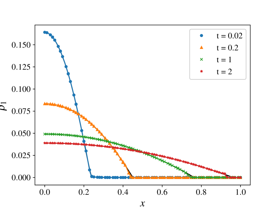
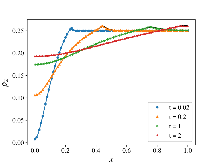
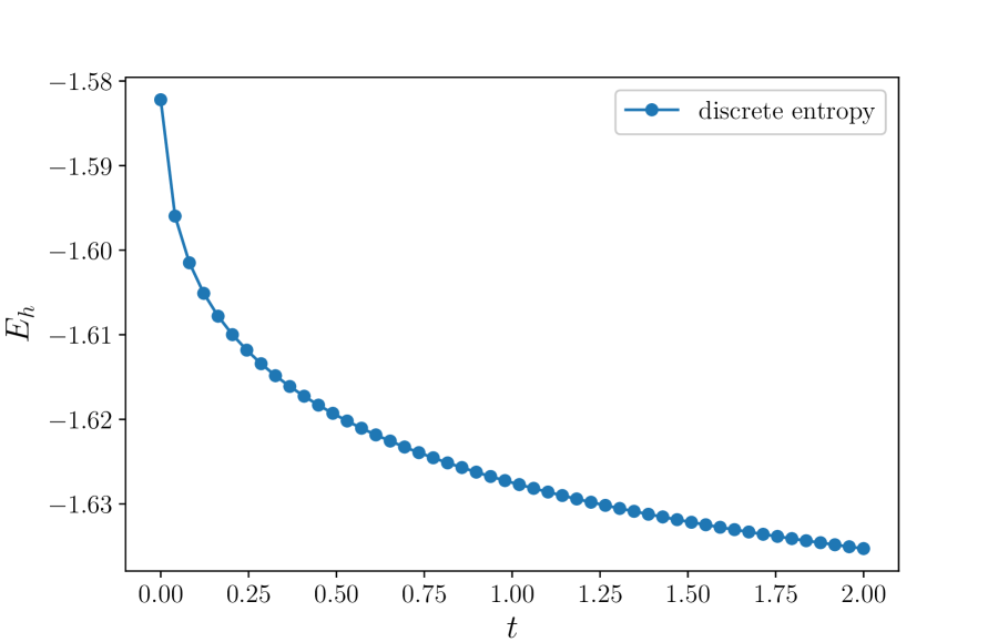
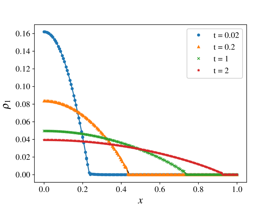
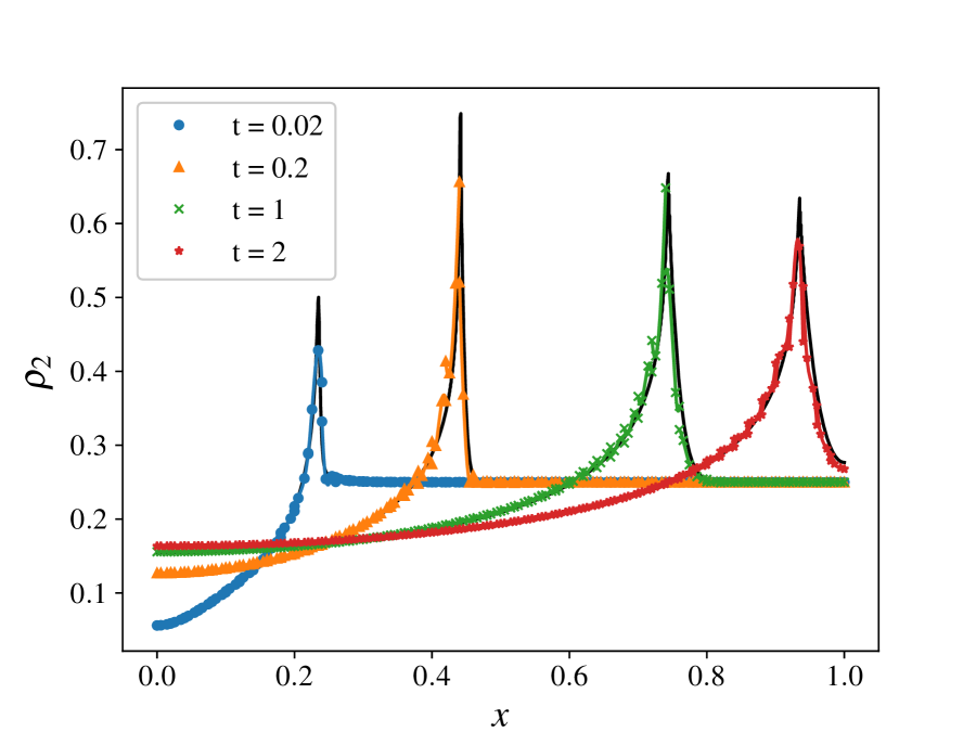
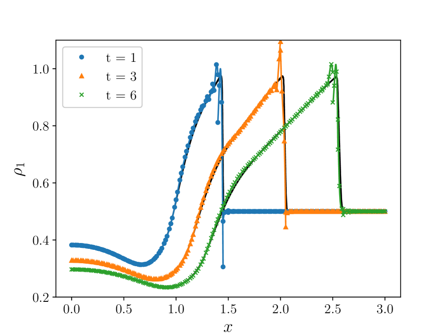
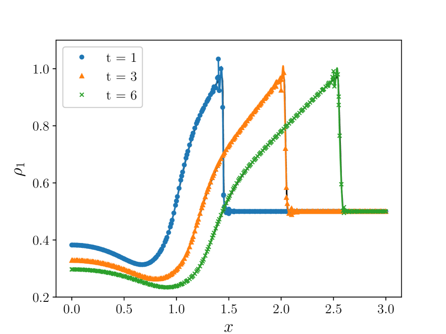
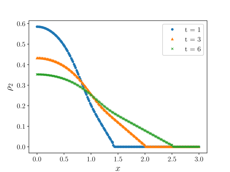
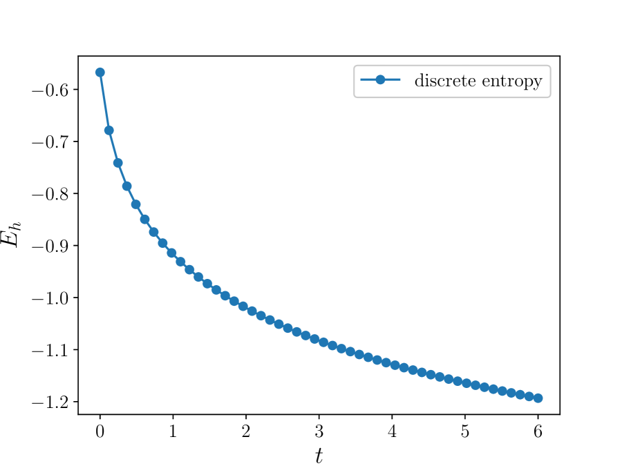
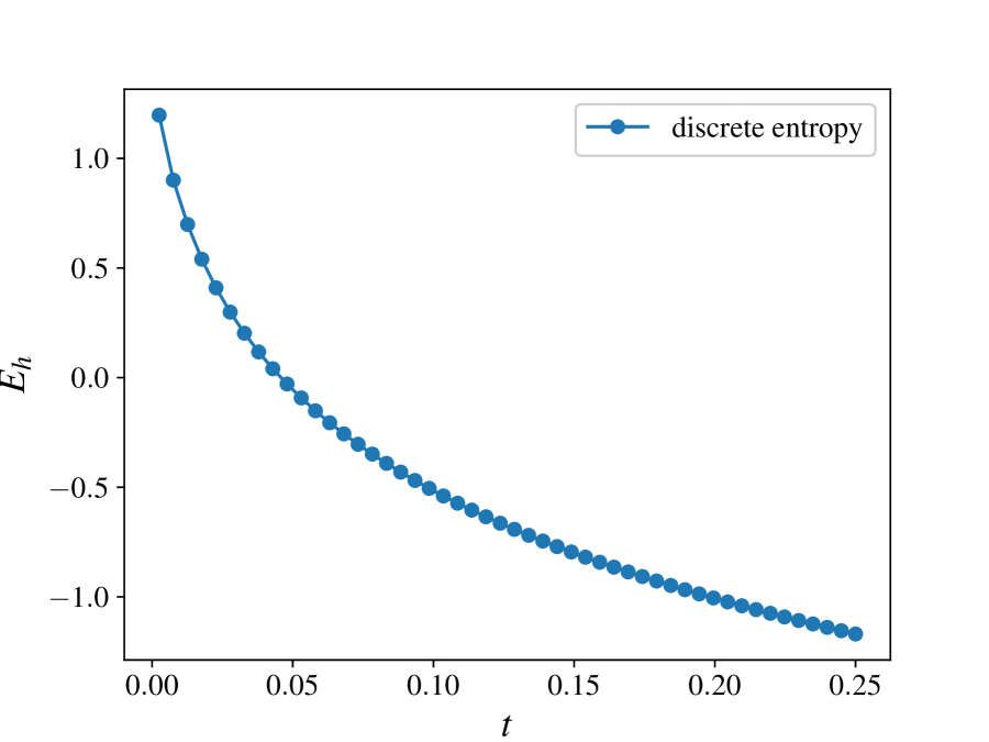
Example 4.3 (Tumor encapsulation).
| (4.2a) | ||||
| (4.2b) | ||||
System (4.2) comes from the tumor encapsulation model proposed by Jackson and Byrne in [25], which describes the formation of a dense, fibrous connective tissue surrounding the benign neoplastic mass. In the system, corresponds to the concentration of tumors, and is the concentration of the surrounding tissue. In [29], the authors pointed out the system can be formulated as a gradient flow with the entropy
if . Then and the corresponding is semi-positive definite with the prescribed parameters. In the numerical test, we firstly consider the case and . The initial condition is set as
The zero-flux boundary condition is applied in the simulation. The computational domain is set as with and respectively. We choose the time step to be . The numerical results are given in Figure 4.1. We then consider problems with a strong cell-induced pressure, with and . These parameters are rescaled from [25] and we drop the source term in their simulation. In the numerical test, instead of is used in the scaling limiter for robustness and all other settings are the same. The numerical results are given in Figure 4.2. Although the system may no long possess a decaying entropy since , it seems that our numerical method still produces satisfying results and captures the sharp leading front of .


Example 4.4 (Surfactant spreading).
We perform numerical simulations of a system modelling the surfactant spreading on a thin viscous film, which can be used for analyzing the delivery of aerosol for curing the respiratory distress syndrome. The system was derived by Jensen and Grotberg in [26] and was then analyzed by Escher et al. in [22]. In this system, represents the film thickness and is the concentration of the surfactant. The parameter corresponds to a gravitational force.
| (4.3a) | ||||
| (4.3b) | ||||
Following the derivation in [22], the system is associated with the following entropy functional
Accordingly, , and . It is shown in [26] that the similarity solutions to (4.3) would develop shocks as . In this numerical test, we consider a weak gravitational effect with . A uniform mesh with is used on the spatial domain . The time step is set as . We apply the zero-flux boundary condition and assume the initial condition to be and . Numerical solutions obtained with and are given in Figure 4.3. Under the same setting without applying positivity-preserving limiter, the solutions blow up shortly after for and for .


5 Two-dimensional numerical tests
In this section, we provide several numerical examples of two-dimensional problems on Cartesian meshes. The accuracy test is given in Example 5.1. Then we apply the numerical scheme to solve the two-dimensional surfactant spreading problem in Example 5.2 and the seawater intrusion model in Example 5.3.
Example 5.1.
We start with the accuracy test and consider the two-dimensional version of Example 4.2 with a source term .
The problem is again associated with the logarithm entropy.
Then and . We assume the exact solution . The source term is computed accordingly. We compute to . The time step is set as for and for .
| error | order | error | order | error | order | ||
| 1 | 10 | 1.185E-01 | - | 5.349E-02 | - | 5.732E-02 | - |
| 20 | 4.656E-02 | 1.35 | 2.147E-02 | 1.32 | 2.265E-02 | 1.34 | |
| 40 | 1.773E-02 | 1.39 | 8.266E-03 | 1.38 | 8.692E-03 | 1.38 | |
| 80 | 6.218E-03 | 1.51 | 2.921E-03 | 1.50 | 3.084E-03 | 1.50 | |
| 2 | 10 | 8.206E-03 | - | 4.362E-03 | - | 8.402E-03 | - |
| 20 | 9.124E-04 | 3.17 | 5.659E-04 | 2.95 | 9.942E-04 | 3.08 | |
| 40 | 1.077E-04 | 3.08 | 7.186E-05 | 2.98 | 1.213E-04 | 3.04 | |
| 80 | 1.315E-05 | 3.03 | 9.068E-06 | 2.99 | 1.515E-05 | 3.00 | |
| 3 | 10 | 9.481E-04 | - | 5.256E-04 | - | 9.990E-04 | - |
| 20 | 1.061E-04 | 3.16 | 5.847E-05 | 3.17 | 1.112E-04 | 3.17 | |
| 40 | 1.128E-05 | 3.23 | 6.169E-06 | 3.25 | 1.216E-05 | 3.19 | |
| 80 | 1.119E-06 | 3.33 | 6.042E-07 | 3.35 | 1.232E-06 | 3.30 | |
| 4 | 10 | 4.685E-05 | - | 2.649E-05 | - | 7.459E-05 | - |
| 20 | 1.212E-06 | 5.27 | 8.159E-07 | 5.02 | 2.837E-06 | 4.72 | |
| 40 | 3.328E-08 | 5.19 | 2.273E-08 | 5.17 | 7.754E-08 | 5.19 |
| error | order | error | order | error | order | ||
| 1 | 10 | 3.848E-01 | - | 1.853E-01 | - | 2.415E-01 | - |
| 20 | 9.608E-02 | 2.00 | 4.397E-02 | 2.08 | 4.372E-02 | 2.47 | |
| 40 | 2.376E-02 | 2.02 | 1.075E-02 | 2.03 | 1.014E-02 | 2.11 | |
| 80 | 5.916E-03 | 2.01 | 2.667E-03 | 2.01 | 2.525E-03 | 2.01 | |
| 2 | 10 | 1.510E-02 | - | 8.132E-03 | - | 2.121E-02 | - |
| 20 | 1.673E-03 | 3.17 | 9.563E-04 | 3.09 | 2.328E-03 | 3.19 | |
| 40 | 1.923E-04 | 3.12 | 1.169E-04 | 3.03 | 2.662E-04 | 3.13 | |
| 80 | 2.294E-05 | 3.07 | 1.453E-05 | 3.01 | 3.192E-05 | 3.06 | |
| 3 | 10 | 8.253E-04 | - | 4.525E-04 | - | 1.449E-03 | - |
| 20 | 4.998E-05 | 4.05 | 2.922E-05 | 3.95 | 1.044E-04 | 3.80 | |
| 40 | 3.075E-06 | 4.02 | 1.850E-06 | 3.98 | 6.675E-06 | 3.97 | |
| 80 | 1.912E-07 | 4.01 | 1.161E-07 | 4.00 | 4.216E-07 | 3.99 | |
| 4 | 10 | 5.174E-05 | - | 3.287E-05 | - | 1.448E-04 | - |
| 20 | 1.683E-06 | 4.94 | 1.127E-06 | 4.87 | 4.972E-06 | 4.86 | |
| 40 | 5.276E-08 | 5.00 | 3.620E-08 | 4.96 | 1.485E-07 | 5.07 |
| error | order | error | order | error | order | ||
|---|---|---|---|---|---|---|---|
| 0 | 10 | 1.082E-03 | - | 6.170E-04 | - | 1.139E-03 | - |
| 20 | 1.328E-04 | 3.07 | 7.682E-05 | 3.01 | 1.373E-04 | 3.05 | |
| 40 | 1.651E-05 | 3.01 | 9.595E-06 | 3.00 | 1.722E-05 | 3.00 | |
| 80 | 2.063E-06 | 3.00 | 1.199E-06 | 3.00 | 2.157E-06 | 3.00 | |
| 10 | 2.505E-04 | - | 1.266E-04 | - | 1.528E-04 | - | |
| 20 | 1.234E-05 | 4.34 | 6.425E-06 | 4.30 | 1.234E-05 | 3.63 | |
| 40 | 6.709E-07 | 4.20 | 3.609E-07 | 4.15 | 9.094E-07 | 3.76 | |
| 80 | 3.923E-08 | 4.10 | 2.178E-08 | 4.05 | 6.480E-08 | 3.81 |
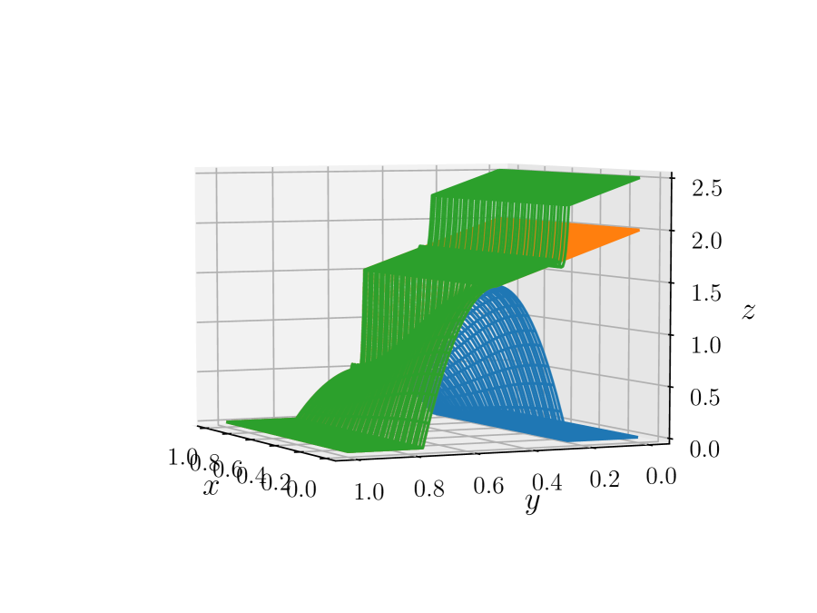
Example 5.2.
In this numerical example, we simulate the two-dimensional surfactant spreading.
| (5.1a) | ||||
| (5.1b) | ||||
Again and correspond to the film thickness and surfactant concentration respectively. The associated entropy is
As before, and . We assume zero-flux boundary condition on and compute to with and . The gravitational coefficient is set as . Numerical results are given in Figure 5.1. The numerical method does capture the sharp transition of the bowl-shaped leading front of , though with oscillations.
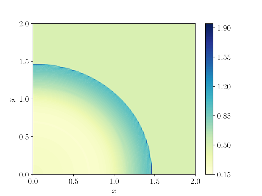

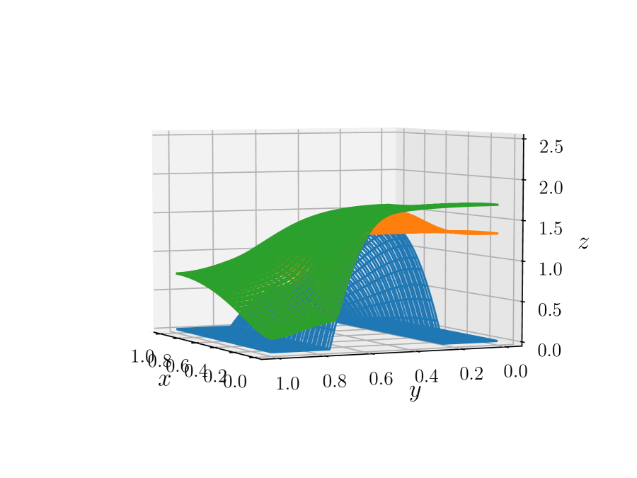
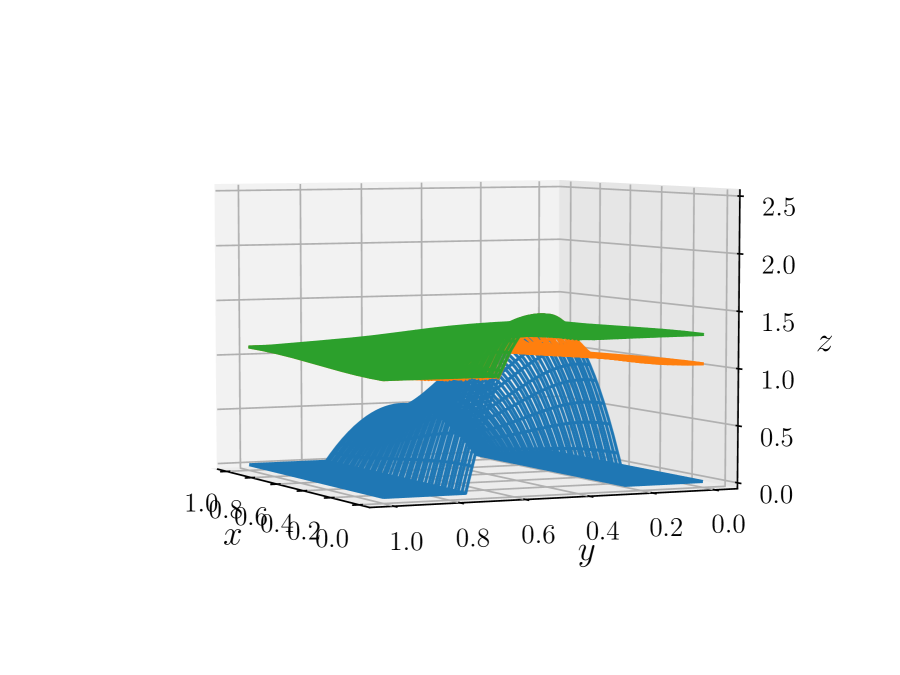
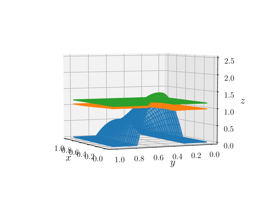
Example 5.3 (Seawater intrusion).
This test case is taken from [37] on solving a cross-diffusion system modelling the seawater intrusion in an unconfined aquifer.
| (5.2a) | ||||
| (5.2b) | ||||
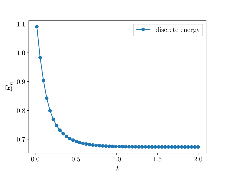
Here gives the impermeable interface between the seawater and the bedrock. The saltwater sits on the bedrock between and . From to is the freshwater, which is immersible with the saltwater. The parameter is the mass density ratio between the freshwater and the saltwater. (5.2) is associated with the energy functional
It can be show that there exists a non-negative solution to (5.2) satisfying the energy decay property
We assume the zero-flux boundary condition and use a square mesh on . We compute to with . The parameter is set as . The initial condition , with
and
is used in our numerical simulation. Here the seabed function is
Numerical solutions at different time are depicted in Figure 5.2. One can see that solutions converge to a steady state as becomes large.
6 Concluding remarks
In this paper, we extend the DG method in [41] to solve cross-diffusion systems with a gradient flow structure. The difficulty is that the non-negativity of solutions is usually an essential part for the entropy stability. One needs to design numerical schemes to preserve the entropy structure, as well as to ensure the positivity of solutions. We adopt the Gauss-Lobatto quadrature rule in the DG method, so that the resulting semi-discrete scheme are subject to an entropy inequality consistent with that of the continuum system. Furthermore, for a class of problems, with a suitable choice of numerical fluxes, the numerical method is compatible with the positivity-preserving procedure established in [43] and [42]. The extension to two-dimensional problems on Cartesian meshes is also discussed. In our numerical tests, we observe that the methods achieve high-order accuracy. Though the convergence rate is reduced with odd-order piecewise polynomials, the optimal rate can be retrieved by imposing larger Lax-Friedrichs constant in the numerical fluxes. Numerical simulations to problems with positivity-preserving issues have also been performed.
Appendix A Fully discrete entropy inequality
Theorem A.1.
Consider the Euler forward time discretization of the one-dimensional scheme (2.2) with central and Lax-Friedrichs fluxes (2.3) on a uniform mesh. Suppose , , and uniformly in for some fixed constants , , and . If , then
Here and are matrix norms of and respectively, is a constant for norm equivalence and is the constant in the inverse estimate.
Proof.
We omit all subscripts and superscripts in this proof.
Here we have applied the mean value theorem and is on the line segment between and . Let . Then
Using the scheme (2.2), we obtain
where lies between and . Our main task is to estimate .
Here and are constants to be determined. Note that defines a norm on . Using norm equivalence and inverse estimates, we have
and
where is a constant not less than in the inverse estimates. Taking and , then we have
Since
one can obtain
Therefore, we conclude that
The proof is completed by substituting the time step restriction into the inequality. ∎
Acknowledgments
JAC was partially supported by the EPSRC grant number EP/P031587/1. JAC would like to thank the Department of Applied Mathematics at Brown University for their kind hospitality and for the support through the IBM Visiting Professorship scheme. CWS was partially supported by ARO grant W911NF-16-1-0103 and NSF grant DMS-1719410.
References
- [1] F. Bassi and S. Rebay. A high-order accurate discontinuous finite element method for the numerical solution of the compressible Navier–Stokes equations. Journal of Computational Physics, 131(2):267–279, 1997.
- [2] J. Berendsen, M. Burger, and J.-P. Pietschmann. On a cross-diffusion model for multiple species with nonlocal interaction and size exclusion. Nonlinear Anal., 159:10–39, 2017.
- [3] M. Bessemoulin-Chatard and F. Filbet. A finite volume scheme for nonlinear degenerate parabolic equations. SIAM Journal on Scientific Computing, 34(5):B559–B583, 2012.
- [4] M. Burger, J. A. Carrillo, and M.-T. Wolfram. A mixed finite element method for nonlinear diffusion equations. Kinetic & Related Models, 3(1):59–83, 2010.
- [5] M. Bruna, M. Burger, H. Ranetbauer, and M.-T. Wolfram. Cross-diffusion systems with excluded-volume effects and asymptotic gradient flow structures. J. Nonlinear Sci., 27(2):687–719, 2017.
- [6] J. A. Carrillo, A. Chertock, and Y. Huang. A finite-volume method for nonlinear nonlocal equations with a gradient flow structure. Communications in Computational Physics, 17(1):233–258, 2015.
- [7] J. A. Carrillo, K. Craig, and F. S. Patacchini. A blob method for diffusion. arXiv preprint arXiv:1709.09195, 2017.
- [8] J. A. Carrillo, F. Filbet, and M. Schmidtchen. Convergence of a finite volume scheme for a system of interacting species with cross-diffusion. arXiv preprint arXiv:1804.04385, 2018.
- [9] J. A. Carrillo, Y. Huang, F. Saverio Patacchini, and G. Wolansky. Numerical study of a particle method for gradient flows. Kinetic & Related Models, 10(3), 2017.
- [10] J. A. Carrillo, B. D’́uring, D. Matthes, and D. McCormick. A Lagrangian scheme for the solution of nonlinear diffusion equations using moving simplex meshes. J. Sci. Comput., 75(3):1463–1499, 2018.
- [11] J. A. Carrillo, and J. S. Moll. Numerical simulation of diffusive and aggregation phenomena in nonlinear continuity equations by evolving diffeomorphisms. SIAM J. Sci. Comput., 31(6):4305–4329, 2009/10.
- [12] J. A. Carrillo, H. Ranetbauer, and M.-T. Wolfram. Numerical simulation of nonlinear continuity equations by evolving diffeomorphisms. J. Comput. Phys., 327:186–202, 2016.
- [13] T. Chen and C.-W. Shu. Entropy stable high order discontinuous Galerkin methods with suitable quadrature rules for hyperbolic conservation laws. Journal of Computational Physics, 345:427–461, 2017.
- [14] Y. Cheng and C.-W. Shu. A discontinuous Galerkin finite element method for time dependent partial differential equations with higher order derivatives. Mathematics of Computation, 77(262):699–730, 2008.
- [15] B. Cockburn, S. Hou, and C.-W. Shu. The Runge–Kutta local projection discontinuous Galerkin finite element method for conservation laws IV: The multidimensional case. Mathematics of Computation, 54(190):545–581, 1990.
- [16] B. Cockburn, S.-Y. Lin, and C.-W. Shu. TVB Runge–Kutta local projection discontinuous Galerkin finite element method for conservation laws III: one-dimensional systems. Journal of Computational Physics, 84(1):90–113, 1989.
- [17] B. Cockburn and C.-W. Shu. TVB Runge–Kutta local projection discontinuous Galerkin finite element method for conservation laws II: General framework. Mathematics of Computation, 52(186):411–435, 1989.
- [18] B. Cockburn and C.-W. Shu. The Runge–Kutta local projection -discontinuous-Galerkin finite element method for scalar conservation laws. ESAIM: Mathematical Modelling and Numerical Analysis, 25(3):337–361, 1991.
- [19] B. Cockburn and C.-W. Shu. The local discontinuous Galerkin method for time-dependent convection-diffusion systems. SIAM Journal on Numerical Analysis, 35(6):2440–2463, 1998.
- [20] B. Cockburn and C.-W. Shu. The Runge–Kutta discontinuous Galerkin method for conservation laws V: multidimensional systems. Journal of Computational Physics, 141(2):199–224, 1998.
- [21] K. Craig and A. Bertozzi. A blob method for the aggregation equation. Mathematics of computation, 85(300):1681–1717, 2016.
- [22] J. Escher, M. Hillairet, P. Laurencot, and C. Walker. Global weak solutions for a degenerate parabolic system modeling the spreading of insoluble surfactant. Indiana University Mathematics Journal, pages 1975–2019, 2011.
- [23] S. Gottlieb, C.-W. Shu, and E. Tadmor. Strong stability-preserving high-order time discretization methods. SIAM Review, 43(1):89–112, 2001.
- [24] S. Hittmeir, H. Ranetbauer, C. Schmeiser, and M.-T. Wolfram. Derivation and analysis of continuum models for crossing pedestrian traffic. Math. Models Methods Appl. Sci., 27(7):1301–1325, 2017.
- [25] T. L. Jackson and H. M. Byrne. A mechanical model of tumor encapsulation and transcapsular spread. Mathematical Biosciences, 180(1-2):307–328, 2002.
- [26] O. Jensen and J. Grotberg. Insoluble surfactant spreading on a thin viscous film: shock evolution and film rupture. Journal of Fluid Mechanics, 240:259–288, 1992.
- [27] O. Junge, D. Matthes, and H. Osberger. A fully discrete variational scheme for solving nonlinear Fokker-Planck equations in multiple space dimensions. SIAM J. Numer. Anal., 55(1):419–443, 2017.
- [28] A. Jüngel. The boundedness-by-entropy method for cross-diffusion systems. Nonlinearity, 28(6):1963, 2015.
- [29] A. Jüngel and I. V. Stelzer. Entropy structure of a cross-diffusion tumor-growth model. Mathematical Models and Methods in Applied Sciences, 22(07):1250009, 2012.
- [30] A. Jüngel and N. Zamponi. Qualitative behavior of solutions to cross-diffusion systems from population dynamics. J. Math. Anal. Appl., 440:794–809, 2016.
- [31] A. Jüngel and N. Zamponi. Analysis of degenerate cross-diffusion population models with volume filling. Ann. Inst. H. Poincaré Anal. Non Linéaire, 34(1):1–29, 2017.
- [32] E. F. Keller and L. A. Segel. Initiation of slime mold aggregation viewed as an instability. Journal of Theoretical Biology, 26(3):399–415, 1970.
- [33] H. Liu and H. Yu. The entropy satisfying discontinuous Galerkin method for Fokker-Planck equations. J. Sci. Comput., 62(3):803–830, 2015.
- [34] H. Liu and Z. Wang. An entropy satisfying discontinuous Galerkin method for nonlinear Fokker–Planck equations. J. Sci. Comput., 68(3):1217–1240, 2016.
- [35] H. Liu and Z. Wang. A free energy satisfying discontinuous Galerkin method for one-dimensional Poisson–Nernst–Planck systems. Journal of Computational Physics, 328:413–437, 2017.
- [36] H. Liu and J. Yan. The direct discontinuous Galerkin (DDG) methods for diffusion problems. SIAM Journal on Numerical Analysis, 47(1):675–698, 2009.
- [37] A. A. H. Oulhaj. A finite volume scheme for a seawater intrusion model with cross-diffusion. In C. Cancès and P. Omnes, editors, Finite Volumes for Complex Applications VIII - Methods and Theoretical Aspects, pages 421–429, Cham, 2017. Springer International Publishing.
- [38] W. H. Reed and T. Hill. Triangular mesh methods for the neutron transport equation. Technical report, Los Alamos Scientific Lab., N. Mex.(USA), 1973.
- [39] N. Shigesada, K. Kawasaki, and E. Teramoto. Spatial segregation of interacting species. Journal of Theoretical Biology, 79(1):83–99, 1979.
- [40] S. Srinivasana, J. Poggiea, and X. Zhang. A positivity-preserving high order discontinuous Galerkin scheme for convection-diffusion equations. Journal of Computational Physics, to appear.
- [41] Z. Sun, J. A. Carrillo, and C.-W. Shu. A discontinuous Galerkin method for nonlinear parabolic equations and gradient flow problems with interaction potentials. Journal of Computational Physics, 352:76–104, 2018.
- [42] X. Zhang. On positivity-preserving high order discontinuous Galerkin schemes for compressible Navier–Stokes equations. Journal of Computational Physics, 328:301–343, 2017.
- [43] X. Zhang and C.-W. Shu. On maximum-principle-satisfying high order schemes for scalar conservation laws. Journal of Computational Physics, 229(9):3091–3120, 2010.