Study of the $D^{0}\to K^{-}\mu^{+}\nu_{\mu}$ dynamics and test of lepton flavor universality with $D^{0}\to K^{-}\ell^{+}\nu_{\ell}$ decays

Abstract

Using $e^{+}e^{-}$ annihilation data of $2.93~{}\mathrm{fb}^{-1}$ collected at center-of-mass energy $\sqrt{s}=3.773$ GeV with the BESIII detector, we measure the absolute branching fraction of $D^{0}\to K^{-}\mu^{+}\nu_{\mu}$ with significantly improved precision: ${\mathcal{B}}_{D^{0}\to K^{-}\mu^{+}\nu_{\mu}}=(3.413\pm 0.019_{\rm stat.}\pm 0.035_{\rm syst.})\%$. Combining with our previous measurement of ${\mathcal{B}}_{D^{0}\to K^{-}e^{+}\nu_{e}}$, the ratio of the two branching fractions is determined to be ${\mathcal{B}}_{D^{0}\to K^{-}\mu^{+}\nu_{\mu}}/{\mathcal{B}}_{D^{0}\to K^{-}e^{+}\nu_{e}}=0.974\pm 0.007_{\rm stat.}\pm 0.012_{\rm syst.}$, which agrees with the theoretical expectation of lepton flavor universality within the uncertainty. A study of the ratio of the two branching fractions in different four-momentum transfer regions is also performed, and no evidence for lepton flavor universality violation is found with current statistics. Taking inputs from global fit in the standard model and lattice quantum chromodynamics separately, we determine $f_{+}^{K}(0)=0.7327\pm 0.0039_{\rm stat.}\pm 0.0030_{\rm syst.}$ and $|V_{cs}|=0.955\pm 0.005_{\rm stat.}\pm 0.004_{\rm syst.}\pm 0.024_{\rm LQCD}$.

In the standard model (SM), lepton flavor universality (LFU) requires equality of couplings between three families of leptons and gauge bosons. Semileptonic (SL) decays of pseudoscalar mesons, well understood in the SM, offer an excellent opportunity to test LFU and search for new physics effects. Recently, various LFU tests in SL $B$ decays were reported at BaBar, Belle and LHCb. The measured branching fraction (BF) ratios ${\mathcal{R}}_{D^{(*)}}^{\tau/\ell}={\mathcal{B}}_{B\to\bar{D}^{(*)}\tau^{+}\nu_{\tau}}/{\mathcal{B}}_{B\to\bar{D}^{(*)}\ell^{+}\nu_{\ell}}$ ($\ell=\mu$, $e$) babar_1 ; babar_2 ; lhcb_1 ; belle2015 ; belle2016 and ${\mathcal{R}}_{K^{(*)}}^{\mu\mu/ee}={\mathcal{B}}_{B\to K^{(*)}\mu^{+}\mu^{-}}/{\mathcal{B}}_{B\to K^{(*)}e^{+}e^{-}}$ lhcb_kee_3 ; lhcb_kee_4 deviate from SM predictions by $3.9\sigma$ HFLAV and 2.1-$2.5\sigma$, respectively. Various models BFajfer2012 ; Fajfer2012 ; Celis2013 ; Crivellin2015 ; Crivellin2016 ; Bauer2016 were proposed to explain these tensions. Precision measurements of SL $D$ decays provide critical and complementary tests of LFU. Reference Fajfer2015 states that observable LFU violations may exist in $D^{0}\to K^{-}\ell^{+}\nu_{\ell}$ decays. In the SM, Ref. Riggio2018 predicts ${\mathcal{R}}_{\mu/e}={\mathcal{B}}_{D^{0}\to K^{-}\mu^{+}\nu_{\mu}}/{\mathcal{B}}_{D^{0}\to K^{-}e^{+}\nu_{e}}=0.975\pm 0.001$. Above $q^{2}=0.1$ GeV${}^{2}/c^{4}$ ($q$ is the total four momentum of $\ell^{+}\nu_{\ell}$), one expects ${\mathcal{R}}_{\mu/e}$ close to 1 with negligible uncertainty ETM2017 . This Letter presents an improved measurement of $D^{0}\to K^{-}\mu^{+}\nu_{\mu}$ charge , and LFU test with $D^{0}\to K^{-}\ell^{+}\nu_{\ell}$ decays in the full kinematic range and various separate $q^{2}$ intervals.

Moreover, experimental studies of the $D^{0}\to K^{-}\ell^{+}\nu_{\ell}$ dynamics help to determine the $c\to s$ quark mixing matrix element $|V_{cs}|$ and the hadronic form factors (FFs) $f_{\pm}^{K}(0)$ Riggio2018 ; Zhang2018 ; Fang2015 . The $D^{0}\to K^{-}e^{+}\nu_{e}$ dynamics was well studied by CLEO-c, Belle, BaBar, and BESIII belle2006 ; cleo2009 ; babar2007 ; bes2015 . However, the $D^{0}\to K^{-}\mu^{+}\nu_{\mu}$ dynamics was only investigated by Belle and FOCUS focus2005 ; belle2006 , with relatively poor precision. By analyzing the $D^{0}\to K^{-}\mu^{+}\nu_{\mu}$ dynamics, we determine $|V_{cs}|$ and $f^{K}_{+}(0)$ incorporating the inputs from global fit in the SM pdg2016 and lattice quantum chromodynamics (LQCD) LQCD . These are critical to test quark mixing matrix unitarity and validate LQCD calculations on FFs. This analysis is performed using 2.93 fb^-1 of data taken at center-of-mass energy $\sqrt{s}=$ 3.773 GeV with the BESIII detector.

Details about the design and performance of the BESIII detector are given in Ref. BESCol . The Monte Carlo (MC) simulated events are generated with a geant4-based geant4 detector simulation software package, boost. An inclusive MC sample, which includes the $D^{0}\bar{D}^{0}$, $D^{+}D^{-}$ and non-$D\bar{D}$ decays of $\psi(3770)$, the initial state radiation (ISR) production of $\psi(3686)$ and $J/\psi$, and the $q\bar{q}$ ($q=u,d,s$) continuum process, along with Bhabha scattering, $\mu^{+}\mu^{-}$ and $\tau^{+}\tau^{-}$ events, is produced at $\sqrt{s}=3.773$ GeV to determine the detection efficiencies and to estimate the potential backgrounds. The production of the charmonium states is simulated by the MC generator kkmc kkmc . The measured decay modes of the charmonium states are generated using evtgen evtgen with BFs from the Particle Data Group (PDG) pdg2016 , and the remaining unknown decay modes are generated by lundcharm lundcharm . The $D^{0}\to K^{-}\mu^{+}\nu_{\mu}$ decay is simulated with the modified pole model MPM .

At $\sqrt{s}=3.773$ GeV, the $\psi(3770)$ resonance decays predominately into $D^{0}\bar{D}^{0}$ or $D^{+}D^{-}$ meson pairs. If a $\bar{D}^{0}$ meson is fully reconstructed by $\bar{D}^{0}\to K^{+}\pi^{-},K^{+}\pi^{-}\pi^{0}$ and $K^{+}\pi^{-}\pi^{-}\pi^{+}$, a $D^{0}$ meson must exist in the recoiling system of the reconstructed $\bar{D}^{0}$ (called the single-tag (ST) $\bar{D}^{0}$). In the presence of the ST $\bar{D}^{0}$, we select and study $D^{0}\to K^{-}\mu^{+}\nu_{\mu}$ decay (called the double-tag (DT) events). The BF of the SL decay is given by

$${\mathcal{B}}_{D^{0}\to K^{-}\mu^{+}\nu_{\mu}}=N_{\mathrm{DT}}/(N_{\mathrm{ST}}^{\rm tot}\times\varepsilon_{\rm SL}),$$ (1)

where $N_{\rm ST}^{\rm tot}$ and $N_{\rm DT}$ are the ST and DT yields, $\varepsilon_{\rm SL}=\varepsilon_{\rm DT}/\varepsilon_{\rm ST}$ is the efficiency of reconstructing $D^{0}\to K^{-}\mu^{+}\nu_{\mu}$ in the presence of the ST $\bar{D}^{0}$, and $\varepsilon_{\rm ST}$ and $\varepsilon_{\rm DT}$ are the efficiencies of selecting ST and DT events.

All charged tracks must originate from the interaction point with a distance of closest approach less than 1 cm in the transverse plane and less than 10 cm along the $z$ axis. Their polar angles ($\theta$) are required to satisfy $|\cos\theta|<0.93$. Charged particle identification (PID) is performed by combining the time-of-flight information and the specific ionization energy loss measured in the main drift chamber. The information of the electromagnetic calorimeter (EMC) is also included to identify muon candidates. Combined confidence levels for electron, muon, pion and kaon hypotheses ($CL_{e}$, $CL_{\mu}$, $CL_{\pi}$ and $CL_{K}$) are calculated individually. Kaon (pion) and muon candidates must satisfy $CL_{K(\pi)}>CL_{\pi(K)}$ and $CL_{\mu}>$ 0.001, $CL_{e}$ and $CL_{K}$, respectively. In addition, the deposited energy in the EMC of the muon is required to be within (0.02, 0.29) GeV. The $\pi^{0}$ meson is reconstructed via $\pi^{0}\to\gamma\gamma$ decay. The energy deposited in the EMC of each photon is required to be greater than 0.025 GeV in the barrel ($|\cos\theta|<0.80$) region or 0.050 GeV in the end cap ($0.86<|\cos\theta|<0.92$) region, and the shower time has to be within 700 ns of the event start time. The $\pi^{0}$ candidates with both photons from the end cap are rejected because of poor resolution. The $\gamma\gamma$ combination with an invariant mass ($M_{\gamma\gamma}$) in the range $(0.115,\,0.150)$ GeV$/c^{2}$ is regarded as a $\pi^{0}$ candidate, and a kinematic fit by constraining the $M_{\gamma\gamma}$ to the $\pi^{0}$ nominal mass pdg2016 is performed to improve the mass resolution. For $\bar{D}^{0}\to K^{+}\pi^{-}$, the backgrounds from cosmic ray events, radiative Bhabha scattering and dimuon events are suppressed with the same requirements as used in Ref. cosmic .

The ST $\bar{D}^{0}$ mesons are identified by the energy difference $\Delta E\equiv E_{\bar{D}^{0}}-E_{\rm beam}$ and the beam-constrained mass $M_{\rm BC}\equiv\sqrt{E_{\mathrm{beam}}^{2}-|\vec{p}_{\bar{D}^{0}}|^{2}}$, where $E_{\mathrm{beam}}$ is the beam energy, and $E_{\bar{D}^{0}}$ and $\vec{p}_{\bar{D}^{0}}$ are the total energy and momentum of the ST $\bar{D}^{0}$ in the $e^{+}e^{-}$ rest frame. If there are multiple combinations in an event, the combination with the smallest $|\Delta E|$ is chosen for each tag mode and for $D^{0}$ and $\bar{D}^{0}$. For one event, there may be up to six ST $D$ candidates selected. To determine the ST yield, we fit the $M_{\rm BC}$ distributions of the accepted candidates after imposing mode dependent $\Delta E$ requirements. The signal is described by the MC-simulated shape convolved with a double-Gaussian function accounting for the resolution difference between data and MC simulation, and the background is modeled by an ARGUS function argus . Fit results are shown in Figs. 1(a-c). The corresponding $\Delta E$ and $M_{\rm BC}$ requirements, ST yields and efficiencies for various ST modes are summarized in Table 1. The total ST yield is $N^{\rm tot}_{\rm ST}=2341408\pm 2056$.

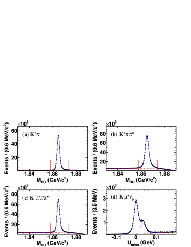
Fig. 1: Fits to (a-c) the $M_{\rm BC}$ distributions for the three ST modes, and (d) the $U_{\rm miss}$ distribution for $D^{0}\to K^{-}\mu^{+}\nu_{\mu}$ candidates. Dots with error bars are data, solid curves show the fit results, dashed curves show the fitted non-peaking background shapes, the dash-dotted curve in (d) is the peaking background shape of $D^{0}\to K^{-}\pi^{+}\pi^{0}$ and the red arrows in (a-c) give the $M_{\rm BC}$ windows.

Table 1: $\Delta E$ and $M_{\rm BC}$ requirements, ST yields $N_{\rm ST}$, ST efficiencies $\varepsilon_{\rm ST}$ and signal efficiencies $\varepsilon_{\rm SL}$ for different ST modes. Uncertainties are statistical only.

ST mode	$\Delta E$ (MeV)	$M_{\rm BC}$ (GeV/$c^{2}$)	$N_{\rm ST}$	$\varepsilon_{\rm ST}$ (%)	$\varepsilon_{\rm SL}$ (%)
$K^{+}\pi^{-}$	$(-29,\,27)$	$(1.858,\,1.874)$	$538865\pm 785$	$65.37\pm 0.09$	$57.74\pm 0.09$
$K^{+}\pi^{-}\pi^{0}$	$(-69,\,38)$	$(1.858,\,1.874)$	$1080050\pm 1532$	$34.67\pm 0.04$	$61.23\pm 0.09$
$K^{+}\pi^{-}\pi^{-}\pi^{+}$	$(-31,\,28)$	$(1.858,\,1.874)$	$722493\pm 1126$	$38.20\pm 0.06$	$56.42\pm 0.09$

Candidates for $D^{0}\to K^{-}\mu^{+}\nu_{\mu}$ must contain two oppositely charged tracks which are identified as a kaon and muon, respectively. The muon must have the same charge as the kaon on the ST side. To suppress the peaking backgrounds from $D^{0}\to K^{-}\pi^{+}(\pi^{0})$, the $K^{-}\mu^{+}$ invariant mass ($M_{K^{-}\mu^{+}}$) is required to be less than 1.56 GeV/$c^{2}$, and the maximum energy of any photon that is not used in the ST selection ($E_{\rm extra~{}\gamma}^{\rm max}$) must be less than 0.25 GeV.

The kinematic quantity $U_{\mathrm{miss}}\equiv E_{\mathrm{miss}}-|\vec{p}_{\mathrm{miss}}|$ is calculated for each event, where $E_{\mathrm{miss}}$ and $\vec{p}_{\mathrm{miss}}$ are the energy and momentum of the missing particle, which can be calculated by $E_{\mathrm{miss}}\equiv E_{\mathrm{beam}}-E_{K^{-}}-E_{\mu^{+}}$ and $\vec{p}_{\mathrm{miss}}\equiv\vec{p}_{D^{0}}-\vec{p}_{K^{-}}-\vec{p}_{\mu^{+}}$ in the $e^{+}e^{-}$ center-of-mass frame, where $E_{K^{-}(\mu^{+})}$ and $\vec{p}_{K^{-}(\mu^{+})}$ are the energy and momentum of the kaon (muon) candidates. To improve the $U_{\mathrm{miss}}$ resolution, the $D^{0}$ energy is constrained to the beam energy and $\vec{p}_{D^{0}}\equiv-\hat{p}_{\bar{D}^{0}}\sqrt{E_{\mathrm{beam}}^{2}-m_{\bar{D}^{0}}^{2}}$, where $\hat{p}_{\bar{D}^{0}}$ is the unit vector in the momentum direction of the ST $\bar{D}^{0}$ and $m_{\bar{D}^{0}}$ is the $\bar{D}^{0}$ nominal mass pdg2016 .

The SL decay yield is obtained from an unbinned fit to the $U_{\mathrm{miss}}$ distribution of the accepted events of data, as shown in Fig. 1 (d). In the fit, the signal, the peaking background of $D^{0}\to K^{-}\pi^{+}\pi^{0}$ decay and other backgrounds are described by the corresponding MC-simulated shapes. The former two are convolved with the same Gaussian function to account for the resolution difference between data and MC simulation. All parameters are left free. The fitted signal yield is $N_{\rm DT}=47100\pm 259$.

The efficiencies of finding $D^{0}\to K^{-}\mu^{+}\nu_{\mu}$ for different ST modes are summarized in Table 1. They are weighted by the ST yields and give the average efficiency $\varepsilon_{\rm SL}=(58.93\pm 0.07)\%$. To verify the reliability of the efficiency, typical distributions of the SL decay, $e.g.$, momenta and $\cos\theta$ of $K^{-}$ and $\mu^{+}$, are checked and good consistency between data and MC simulation has been found (See Fig. 1 of Ref. app ).

By inserting $N_{\rm DT}$, $\varepsilon_{\rm SL}$ and $N_{\rm ST}^{\rm tot}$ into Eq. (1), one obtains

$${\mathcal{B}}_{D^{0}\to K^{-}\mu^{+}\nu_{\mu}}=(3.413\pm 0.019_{\rm stat.}\pm 0.035_{\rm syst.})\%.$$

The systematic uncertainties in the BF measurement are described as follows. The uncertainty in $N_{\rm ST}^{\rm tot}$ is taken as 0.5% by examining the changes of the fitted yields by varying the fit range, the signal shape and the endpoint of the ARGUS function. The efficiencies of muon and kaon tracking (PID) are studied with $e^{+}e^{-}\to\gamma\mu^{+}\mu^{-}$ events and DT hadronic events, respectively. The uncertainties of tracking and PID efficiencies each are assigned as 0.3% per kaon or muon. The differences of the momentum and $\cos\theta$ distributions between $D^{0}\to K^{-}\mu^{+}\nu_{\mu}$ and the control samples have been considered. The uncertainty of the $E_{\rm extra~{}\gamma}^{\rm max}$ requirement is estimated to be 0.1% by analyzing the DT hadronic events. The uncertainty in the $M_{K^{-}\mu^{+}}$ requirement is estimated with the alternative $M_{K^{-}\mu^{+}}$ requirements of 1.51 or 1.61 GeV/$c^{2}$, and the larger change on the BF 0.4% is taken as the systematic uncertainty. The uncertainty of the $U_{\rm miss}$ fit is estimated to be 0.5% by applying different fit ranges, and signal and background shapes. The uncertainty of the limited MC size is 0.1%. The uncertainty in the MC model is estimated to be 0.1%, which is the difference between our nominal DT efficiency and that determined by reweighting the $q^{2}$ distribution of the signal MC events to data with the obtained FF parameters (See below). The total uncertainty is 1.02%, which is obtained by adding these uncertainties in quadrature.

The BFs of $D^{0}\to K^{-}\mu^{+}\nu_{\mu}$ and $\bar{D}^{0}\to K^{+}\mu^{-}\bar{\nu}_{\mu}$ are measured separately. The results are $\mathcal{B}_{D^{0}\to K^{-}\mu^{+}\nu_{\mu}}=(3.433\pm 0.026_{\rm stat.}\pm 0.039_{\rm syst.})\%$ and $\mathcal{B}_{\bar{D}^{0}\to K^{+}\mu^{-}\bar{\nu}_{\mu}}=(3.392\pm 0.027_{\rm stat.}\pm 0.034_{\rm syst.})\%$. The BF asymmetry is determined to be ${\mathcal{A}}=\frac{{\mathcal{B}}_{D^{0}\to K^{-}\mu^{+}\nu_{\mu}}-{\mathcal{B}}_{\bar{D}^{0}\to K^{+}\mu^{-}\bar{\nu}_{\mu}}}{{\mathcal{B}}_{D^{0}\to K^{-}\mu^{+}\nu_{\mu}}+{\mathcal{B}}_{\bar{D}^{0}\to K^{+}\mu^{-}\bar{\nu}_{\mu}}}=(0.6\pm 0.6_{\rm stat.}\pm 0.8_{\rm syst.})\%$, and no asymmetry in the BFs of $D^{0}\to K^{-}\mu^{+}\nu_{\mu}$ and $\bar{D}^{0}\to K^{+}\mu^{-}\bar{\nu}_{\mu}$ decays is found. All the systematic uncertainties except for those in the $E_{\rm extra~{}\gamma}^{\rm max}$ requirement and MC model are studied separately and are not canceled out in the BF asymmetry calculation.

The $D^{0}\to K^{-}\mu^{+}\nu_{\mu}$ dynamics is studied by dividing the SL candidate events into various $q^{2}$ intervals. The measured partial decay rate (PDR) in the $i$-th $q^{2}$ interval, $\Delta\Gamma_{\rm msr}^{i}$, is determined by

$$\Delta\Gamma^{i}_{\rm msr}\equiv\int_{i}(d\Gamma/dq^{2})dq^{2}=N_{\mathrm{pro}}^{i}/(\tau_{D^{0}}\times N_{\mathrm{ST}}^{\rm tot}),$$ (2)

where $N_{\mathrm{pro}}^{i}$ is the SL decay signal yield produced in the $i$-th $q^{2}$ interval, $\tau_{D^{0}}$ is the $D^{0}$ lifetime and $N_{\mathrm{ST}}^{\rm tot}$ is the ST yield. The signal yield produced in the $i$-th $q^{2}$ interval in data is calculated by

$$N_{\mathrm{pro}}^{i}=\sum_{j}^{N_{\mathrm{intervals}}}(\varepsilon^{-1})_{ij}N_{\mathrm{obs}}^{j},$$ (3)

where the observed DT yield in the $j$-th $q^{2}$ interval $N_{\rm obs}^{j}$ is obtained from the similar fit to the corresponding $U_{\mathrm{miss}}$ distribution of data (See Fig. 2 of Ref. app ). $\varepsilon$ is the efficiency matrix (Table 1 of Ref. app ), which is obtained by analyzing the signal MC events and is given by

$$\varepsilon_{ij}=\sum_{k}(1/N_{\rm ST}^{\rm tot})\times[(N^{ij}_{\mathrm{rec}}\times N_{\rm ST})/(N^{j}_{\mathrm{gen}}\times\varepsilon_{\mathrm{ST}})]_{k},$$ (4)

where $N^{ij}_{\mathrm{rec}}$ is the DT yield generated in the $j$-th $q^{2}$ interval and reconstructed in the $i$-th $q^{2}$ interval, $N^{j}_{\mathrm{gen}}$ is the total signal yield generated in the $j$-th $q^{2}$ interval, and the index $k$ denotes the $k$-th ST mode. The measured PDRs are shown in Fig. 2 (a) and details can be found in Table 2 of Ref. app .

The FF is parametrized as the series expansion parameterization SEM (SEP), which has been shown to be consistent with constraints from QCD bes2015 ; cleo2009 ; babar2015 . The 2-parameter SEP is chosen and is given by

$$f^{K}_{+}(t)=\frac{1}{P(t)\Phi(t,t_{0})}\frac{f^{K}_{+}(0)P(0)\Phi(0,t_{0})}{1+r_{1}(t_{0})z(0,t_{0})}(1+r_{1}(t_{0})[z(t,t_{0})]).$$ (5)

Here, $P(t)=z(t,m_{D^{*}_{s}}^{2})$ and $\Phi$ is given by

$$\begin{array}[]{l}\displaystyle\Phi(t,t_{0})=\sqrt{\frac{1}{24\pi\chi_{V}}}(\frac{t_{+}-t}{t_{+}-t_{0}})^{1/4}(\sqrt{t_{+}-t}+\sqrt{t_{+}})^{-5}\\ \displaystyle\times(\sqrt{t_{+}-t}+\sqrt{t_{+}-t_{0}})(\sqrt{t_{+}-t}+\sqrt{t_{+}-t_{-}})^{3/2}\\ \displaystyle\times(t_{+}-t)^{3/4},\end{array}$$ (6)

where $z(t,t_{0})=\frac{\sqrt{t_{+}-t}-\sqrt{t_{+}-t_{0}}}{\sqrt{t_{+}-t}+\sqrt{t_{+}-t_{0}}}$, $t_{\pm}=(m_{D}\pm m_{K})^{2}$, $t_{0}=t_{+}(1-\sqrt{1-t_{-}/t_{+}})$, $m_{D}$ and $m_{K}$ are the masses of $D$ and $K$ particles, $m_{D_{s}^{*}}$ is the pole mass of the vector FF accounting for the strong interaction between $D$ and $K$ mesons and usually taken as the mass of the lowest lying $c\bar{s}$ vector meson $D_{s}^{*}$ pdg2016 , and $\chi_{V}$ can be obtained from dispersion relations using perturbative QCD chiV .

The PDRs are fitted by assuming the ratio $f_{+}^{K}(q^{2})/f_{-}^{K}(q^{2})$ to be independent of $q^{2}$, and minimizing the $\chi^{2}$ constructed as

$$\chi^{2}=\sum_{i,j=1}^{N_{\mathrm{intervals}}}(\Delta\Gamma^{i}_{\mathrm{msr}}-\Delta\Gamma^{i}_{\mathrm{exp}})C_{ij}^{-1}(\Delta\Gamma^{j}_{\mathrm{msr}}-\Delta\Gamma^{j}_{\mathrm{exp}}),$$ (7)

where $\Delta\Gamma^{i}_{\rm exp}$ is the expected PDR in the $i$-th $q^{2}$ interval given by ddr ; ddr2

$$\Delta\Gamma^{i}_{\rm exp} =\int_{i}\frac{G_{F}^{2}|V_{cs}|^{2}}{8\pi^{3}m_{D}}|\vec{p}_{K}||f_{+}^{K}(q^{2})|^{2}(\frac{W_{0}-E_{K}}{F_{0}})^{2}$$

$$\times[\frac{1}{3}m_{D}|\vec{p}_{K}|^{2}+\frac{m_{\ell}^{2}}{8m_{D}}(m_{D}^{2}+m_{K}^{2}+2m_{D}E_{K})$$

$$+\frac{1}{3}m_{\ell}^{2}\frac{|\vec{p}_{K}|^{2}}{F_{0}}+\frac{1}{4}m_{\ell}^{2}\frac{m_{D}^{2}-m_{K}^{2}}{m_{D}}\mathrm{Re}(\frac{f^{K}_{-}(q^{2})}{f^{K}_{+}(q^{2})})$$

$$+\frac{1}{4}m_{\ell}^{2}F_{0}|\frac{f^{K}_{-}(q^{2})}{f^{K}_{+}(q^{2})}|^{2}]dq^{2},$$ (8)

and $C_{ij}=C_{ij}^{\mathrm{stat}}+C_{ij}^{\mathrm{syst}}$ is the covariance matrix of the measured PDRs among $q^{2}$ intervals. In Eq. (8), $G_{F}$ is the Fermi coupling constant; $m_{\ell}$ is the mass of the lepton; $|\vec{p}_{K}|$ and $E_{K}$ are the momentum and energy of the kaon in the $D$ rest frame; $W_{0}=(m_{D}^{2}+m_{K}^{2}-m_{\ell}^{2})/(2m_{D})$ is the maximum energy of the kaon in the $D$ rest frame; and $F_{0}=W_{0}-E_{K}+m_{\ell}^{2}/(2m_{D})=q^{2}/(2m_{D})$. The statistical covariance matrix (Table 3 of Ref. app ) is constructed as

$$C_{ij}^{\rm stat}=(\frac{1}{\tau_{D^{0}}N_{\mathrm{ST}}^{\rm tot}})^{2}\sum_{\alpha}\varepsilon_{i\alpha}^{-1}\varepsilon_{j\alpha}^{-1}(\sigma(N_{\mathrm{obs}}^{\alpha}))^{2}.$$ (9)

The systematic covariance matrix (Table 4 of Ref. app ) is obtained by summing all the covariance matrices for each source of systematic uncertainty. In general, it has the form

$$C_{ij}^{\mathrm{syst}}=\delta(\Delta\Gamma^{i}_{\rm msr})\delta(\Delta\Gamma^{j}_{\rm msr}),$$ (10)

where $\delta(\Delta\Gamma^{i}_{\rm msr})$ is the systematic uncertainty of the PDR in the $i$-th $q^{2}$ interval. The systematic uncertainties in $N_{\rm ST}^{\rm tot}$, $\tau_{D^{0}}$ and $E_{\rm extra~{}\gamma}^{\rm max}$ requirement are considered to be fully correlated across $q^{2}$ intervals while others are studied separately in each $q^{2}$ interval with the same method used in the BF measurement.

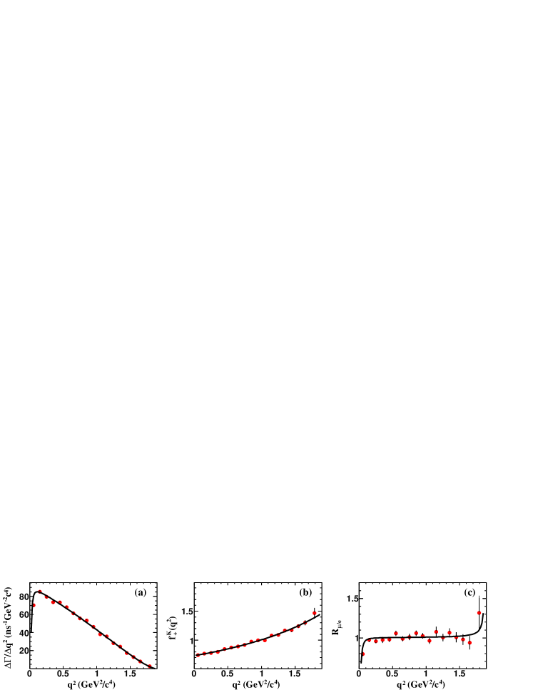
Fig. 2: (a) Fit to the PDRs, (b) projection to $f_{+}^{K}(q^{2})$ for $D^{0}\to K^{-}\mu^{+}\nu_{\mu}$ and (c) the measured ${\mathcal{R}}_{\mu/e}$ in each $q^{2}$ interval. Dots with error bars are data. Solid curves are the fit, the projection or the ${\mathcal{R}}_{\mu/e}$ expected with the parameters in Ref. ETM2017 where the uncertainty is negligible due to strong correlations in hadronic FFs.

Figures 2(a) and (b) show the fit to the PDRs of $D^{0}\to K^{-}\mu^{+}\nu_{\mu}$ and the projection to $f^{K}_{+}(q^{2})$. The goodness of fit is $\chi^{2}/{\rm NDOF}=15.0/15$, where NDOF is the number of degrees of freedom. From the fit, we obtain the product of $f_{+}^{K}(0)|V_{cs}|=0.7133\pm 0.0038_{\rm stat.}\pm 0.0030_{\rm syst.}$, the first order coefficient $r_{1}=-1.90\pm 0.21_{\rm stat.}\pm 0.07_{\rm syst.}$ and the FF ratio $f_{-}^{K}/f_{+}^{K}=-0.6\pm 0.8_{\rm stat.}\pm 0.2_{\rm syst.}$. The nominal fit parameters are taken from the results obtained by fitting with the combined statistical and systematic covariance matrix, and the statistical uncertainties of the fit parameters are taken from the fit with only the statistical covariance matrix. For each parameter, the systematic uncertainty is obtained by calculating the quadratic difference of uncertainties between these two fits.

Combining ${\mathcal{B}}_{D^{0}\to K^{-}\mu^{+}\nu_{\mu}}$ with our previous measurement ${\mathcal{B}}_{D^{0}\to K^{-}e^{+}\nu_{e}}=(3.505\pm 0.014_{\rm stat.}\pm 0.033_{\rm syst.})\%$ bes2015 gives ${\mathcal{R}}_{\mu/e}=0.974\pm 0.007_{\rm stat.}\pm 0.012_{\rm syst.}$, which agrees with the theoretical calculations with LQCD ETM2017 ; Riggio2018 and an SM quark model Soni2017 . Additionally, we determine ${\mathcal{R}}_{\mu/e}$ in each $q^{2}$ interval, as shown in Fig. 2(c), where the error bars include both statistical and the uncanceled systematic uncertainties. In the ${\mathcal{R}}_{\mu/e}$ calculation, the uncertainties in $N_{\rm ST}^{\rm tot}$, $\tau_{D^{0}}$ as well as the tracking and PID efficiencies of the kaon cancel. Below $q^{2}=0.1$ GeV${}^{2}/c^{4}$, ${\mathcal{R}}_{\mu/e}$ is significantly lower than 1 due to smaller phase space for $D^{0}\to K^{-}\mu^{+}\nu_{\mu}$ with nonzero muon mass that cannot be neglected. Above $0.1$ GeV${}^{2}/c^{4}$, ${\mathcal{R}}_{\mu/e}$ is close to 1. They are consistent with the SM prediction, and no deviation larger than 2$\sigma$ is observed.

In summary, by analyzing $2.93~{}\mathrm{fb}^{-1}$ of data collected at $\sqrt{s}=3.773$ GeV with the BESIII detector, we present an improved measurement of the absolute BF of the SL decay $D^{0}\to K^{-}\mu^{+}\nu_{\mu}$. Our result is consistent with the PDG value pdg2016 and improves its precision by a factor of three. Combining the previous BESIII measurements of $D^{0}\to K^{-}e^{+}\nu_{e}$, we calculate ${\mathcal{R}}_{\mu/e}$ ratios in the full $q^{2}$ range and various $q^{2}$ intervals. No significant evidence of LFU violation is found with current statistics and systematic uncertainties. By fitting the PDRs of this decay, we obtain $f_{+}^{K}(0)|V_{cs}|=0.7133\pm 0.0038_{\rm stat.}\pm 0.0029_{\rm syst.}$. Using $|V_{cs}|$ given by global fit in the SM pdg2016 yields $f_{+}^{K}(0)=0.7327\pm 0.0039_{\rm stat.}\pm 0.0030_{\rm syst.}$, while using the $f_{+}^{K}(0)$ calculated in LQCD LQCD results in $|V_{cs}|=0.955\pm 0.005_{\rm stat.}\pm 0.004_{\rm syst.}\pm 0.024_{\rm LQCD}$. These results are consistent with our measurements using $D^{0(+)}\to\bar{K}e^{+}\nu_{e}$ bes2015 ; bes3_ksev ; bes3_klev and $D_{s}^{+}\to\mu^{+}\nu_{\mu}$ bes3_muv within uncertainties and are important to test the LQCD calculation of $f^{K}_{+}(0)$ LQCD ; MILC ; ETM2017 and quark mixing matrix unitarity with better accuracy.

The BESIII collaboration thanks the staff of BEPCII and the IHEP computing center for their strong support. This work is supported in part by National Key Basic Research Program of China under Contract No. 2015CB856700; National Natural Science Foundation of China (NSFC) under Contracts Nos. 11305180, 11775230, 11235011, 11335008, 11425524, 11625523, 11635010; the Chinese Academy of Sciences (CAS) Large-Scale Scientific Facility Program; the CAS Center for Excellence in Particle Physics (CCEPP); Joint Large-Scale Scientific Facility Funds of the NSFC and CAS under Contracts Nos. U1632109, U1332201, U1532257, U1532258; CAS under Contracts Nos. KJCX2-YW-N29, KJCX2-YW-N45, QYZDJ-SSW-SLH003; 100 Talents Program of CAS; National 1000 Talents Program of China; INPAC and Shanghai Key Laboratory for Particle Physics and Cosmology; German Research Foundation DFG under Contracts Nos. Collaborative Research Center CRC 1044, FOR 2359; Istituto Nazionale di Fisica Nucleare, Italy; Koninklijke Nederlandse Akademie van Wetenschappen (KNAW) under Contract No. 530-4CDP03; Ministry of Development of Turkey under Contract No. DPT2006K-120470; National Science and Technology fund; The Swedish Research Council; U. S. Department of Energy under Contracts Nos. DE-FG02-05ER41374, DE-SC-0010118, DE-SC-0010504, DE-SC-0012069; University of Groningen (RuG) and the Helmholtzzentrum fuer Schwerionenforschung GmbH (GSI), Darmstadt; WCU Program of National Research Foundation of Korea under Contract No. R32-2008-000-10155-0.

Supplemental material

Figure 1 shows the comparisons of some typical distributions for $D^{0}\to K^{-}\mu^{+}\nu_{\mu}$ candidate events between data and MC simulation.

Figure 2 shows the fits to the $U_{\rm miss}$ distributions for $D^{0}\to K^{-}\mu^{+}\nu_{\mu}$ candidate events of data in 18 $q^{2}$ intervals.

Table 1 gives the weighted efficiency matrix for all three single tag modes for the reconstruction of $D^{0}\to K^{-}\mu^{+}\nu_{\mu}$ events.

Table 2 presents the number of reconstructed events $N_{\rm obs}^{i}$ obtained from the $U_{\rm miss}$ fits as shown in Fig. 2, the number of produced events $N_{\rm pro}^{i}$, the measured PDR $\Delta\Gamma_{\rm msr}^{i}$ and ${\mathcal{R}}_{\mu/e}$ in each $q^{2}$ interval.

Tables 3 and 4 summarize the statistical and systematic covariance matrices for the measured PDRs in different $q^{2}$ intervals, respectively.

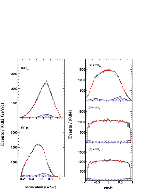
Fig. 1: Comparisons between data and MC simulation of distributions of the kaon and muon momentum and $\cos\theta$ as well as $\cos\theta_{W_{\mu}}$ for $D^{0}\to K^{-}\mu^{+}\nu_{\mu}$ candidate events, where $\theta_{W_{\mu}}$ is the angle between the direction of the virtual $W^{+}$ boson in the $D^{0}$ rest frame and the momentum of muon in the $W^{+}$ rest frame. These events satisfy $-0.06<U_{\rm miss}<0.02$ GeV. The red dots with error bars denote data, the solid histograms are the MC simulated signal plus background and the cross-hatched histograms are the MC simulated background only.

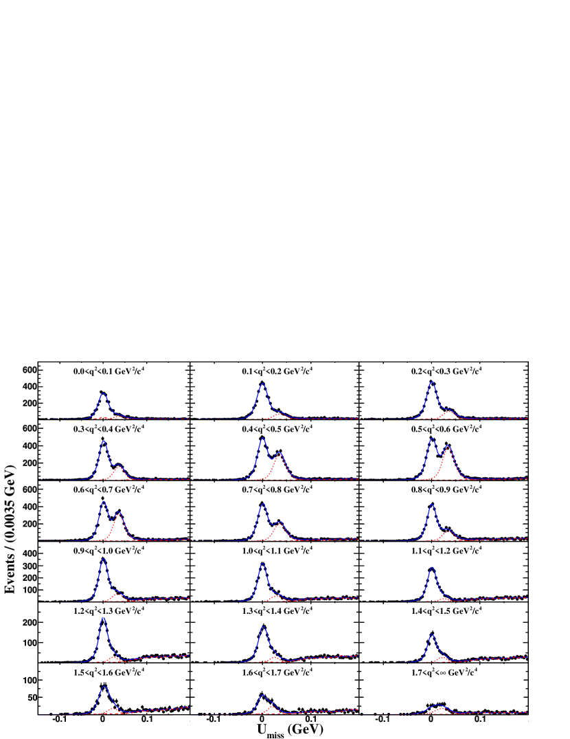
Fig. 2: Fits to $U_{\rm miss}$ distributions in each reconstructed $q^{2}$ bins of data, where the dots with error bars are data, the blue solid curve is the best fit, the red dotted curve is the $D^{0}\to K^{-}\pi^{+}\pi^{0}$ peaking background and the red dashed curve is the combinatorial background.

Table 1: Weighted efficiency matrix for all three single tag modes, where $\varepsilon_{ij}$ represents the efficiency of events generated in the $j$-th $q^{2}$ interval and reconstructed in the $i$-th $q^{2}$ interval.

$\varepsilon_{ij}~{}(\%)$	1	2	3	4	5	6	7	8	9	10	11	12	13	14	15	16	17	18
1	45.49	1.35	0.02	0.01	0.00	0.00	0.00	0.00	0.00	0.00	0.00	0.00	0.00	0.00	0.00	0.00	0.00	0.00
2	1.80	45.09	2.05	0.03	0.01	0.00	0.00	0.00	0.00	0.00	0.00	0.00	0.00	0.00	0.00	0.00	0.00	0.00
3	0.04	1.95	46.76	2.56	0.05	0.01	0.01	0.00	0.00	0.00	0.00	0.00	0.00	0.00	0.00	0.00	0.00	0.00
4	0.02	0.06	2.48	49.30	3.01	0.08	0.02	0.01	0.00	0.00	0.00	0.00	0.00	0.00	0.00	0.00	0.00	0.00
5	0.01	0.02	0.09	2.95	51.96	3.31	0.10	0.02	0.01	0.01	0.00	0.00	0.00	0.00	0.00	0.00	0.00	0.00
6	0.00	0.01	0.03	0.11	3.33	54.37	3.57	0.12	0.04	0.02	0.01	0.00	0.00	0.00	0.00	0.00	0.00	0.00
7	0.00	0.01	0.02	0.04	0.13	3.66	56.65	3.80	0.14	0.04	0.02	0.01	0.00	0.00	0.00	0.00	0.00	0.00
8	0.00	0.00	0.01	0.02	0.05	0.17	3.92	58.23	3.78	0.17	0.06	0.03	0.01	0.00	0.00	0.00	0.00	0.00
9	0.00	0.00	0.01	0.01	0.02	0.06	0.19	4.07	59.44	3.89	0.17	0.07	0.02	0.01	0.00	0.00	0.00	0.00
10	0.00	0.00	0.00	0.01	0.01	0.02	0.07	0.20	4.04	59.52	3.72	0.19	0.07	0.03	0.00	0.00	0.00	0.00
11	0.00	0.00	0.00	0.00	0.01	0.02	0.03	0.07	0.22	3.96	59.13	3.61	0.19	0.06	0.01	0.01	0.00	0.00
12	0.00	0.00	0.00	0.00	0.00	0.01	0.01	0.03	0.08	0.24	3.87	58.83	3.36	0.20	0.06	0.01	0.00	0.00
13	0.00	0.00	0.00	0.00	0.00	0.00	0.01	0.01	0.03	0.07	0.25	3.73	57.92	3.16	0.16	0.04	0.00	0.00
14	0.00	0.00	0.00	0.00	0.00	0.00	0.00	0.00	0.01	0.02	0.07	0.24	3.48	56.60	2.94	0.12	0.02	0.00
15	0.00	0.00	0.00	0.00	0.00	0.00	0.00	0.00	0.00	0.00	0.02	0.06	0.24	3.35	55.35	2.59	0.09	0.00
16	0.00	0.00	0.00	0.00	0.00	0.00	0.00	0.00	0.00	0.00	0.01	0.01	0.05	0.19	3.01	52.79	2.25	0.06
17	0.00	0.00	0.00	0.00	0.00	0.00	0.00	0.00	0.00	0.00	0.00	0.00	0.01	0.03	0.14	2.47	49.49	1.63
18	0.00	0.00	0.00	0.00	0.00	0.00	0.00	0.00	0.00	0.00	0.00	0.00	0.00	0.00	0.01	0.07	1.80	36.80

Table 2: The PDR of $D^{0}\to K^{-}\mu^{+}\nu_{\mu}$ and ${\mathcal{R}}_{\mu/e}$ in each $q^{2}$ bin of data, where uncertainties of PRDs are statistical only.

$i$	$q^{2}$ $(\mathrm{GeV}^{2}/c^{4})$	$N_{\mathrm{obs}}^{i}$	$N_{\mathrm{pro}}^{i}$	$\Delta\Gamma^{i}_{\rm msr}$ $(\mathrm{ns^{-1}})$	${\mathcal{R}}_{\mu/e}$
1	(0.0, 0.1)	2834.1$\pm$63.3	5984.4$\pm$139.3	6.232$\pm$0.145	0.796$\pm$0.027
2	(0.1, 0.2)	3952.1$\pm$71.0	8172.3$\pm$158.1	8.511$\pm$0.165	0.973$\pm$0.026
3	(0.2, 0.3)	3918.6$\pm$70.7	7636.2$\pm$152.2	7.953$\pm$0.158	0.959$\pm$0.026
4	(0.3, 0.4)	3901.2$\pm$71.8	7073.8$\pm$147.0	7.367$\pm$0.153	0.974$\pm$0.037
5	(0.4, 0.5)	4099.6$\pm$77.6	7037.5$\pm$150.9	7.329$\pm$0.157	0.979$\pm$0.029
6	(0.5, 0.6)	4024.5$\pm$78.4	6545.0$\pm$145.9	6.816$\pm$0.152	1.057$\pm$0.034
7	(0.6, 0.7)	3806.2$\pm$75.2	5892.6$\pm$134.5	6.137$\pm$0.140	0.990$\pm$0.031
8	(0.7, 0.8)	3575.2$\pm$70.2	5363.0$\pm$122.3	5.585$\pm$0.127	1.012$\pm$0.039
9	(0.8, 0.9)	3460.2$\pm$67.4	5115.8$\pm$114.9	5.328$\pm$0.120	1.060$\pm$0.034
10	(0.9, 1.0)	3022.3$\pm$64.1	4455.8$\pm$109.1	4.640$\pm$0.114	1.026$\pm$0.035
11	(1.0, 1.1)	2497.2$\pm$58.4	3671.0$\pm$100.1	3.823$\pm$0.104	0.963$\pm$0.036
12	(1.1, 1.2)	2279.4$\pm$60.4	3437.4$\pm$103.9	3.580$\pm$0.108	1.076$\pm$0.068
13	(1.2, 1.3)	1801.0$\pm$54.6	2727.6$\pm$95.3	2.841$\pm$0.099	1.004$\pm$0.047
14	(1.3, 1.4)	1483.7$\pm$52.0	2340.3$\pm$92.8	2.437$\pm$0.097	1.065$\pm$0.057
15	(1.4, 1.5)	1051.2$\pm$45.6	1680.4$\pm$83.1	1.750$\pm$0.087	1.008$\pm$0.064
16	(1.5, 1.6)	727.1$\pm$32.1	1235.5$\pm$61.4	1.287$\pm$0.064	0.979$\pm$0.067
17	(1.6, 1.7)	425.2$\pm$25.9	774.3$\pm$52.7	0.806$\pm$0.055	0.940$\pm$0.086
18	(1.7, $\infty$)	191.7$\pm$22.0	479.5$\pm$59.9	0.499$\pm$0.062	1.318$\pm$0.217

Table 3: Statistical covariance density matrix for the measured PDRs of $D^{0}\to K^{-}\mu^{+}\nu_{\mu}$ in different $q^{2}$ intervals.

$\rho_{ij}$	1	2	3	4	5	6	7	8	9	10	11	12	13	14	15	16	17	18
1	1.000	-0.069	0.003	-0.001	0.000	0.000	0.000	0.000	0.000	0.000	0.000	0.000	0.000	0.000	0.000	0.000	0.000	0.000
2	-0.069	1.000	-0.087	0.005	-0.001	0.000	0.000	0.000	0.000	0.000	0.000	0.000	0.000	0.000	0.000	0.000	0.000	0.000
3	0.003	-0.087	1.000	-0.105	0.006	-0.001	0.000	0.000	0.000	0.000	0.000	0.000	0.000	0.000	0.000	0.000	0.000	0.000
4	-0.001	0.005	-0.105	1.000	-0.117	0.008	-0.001	0.000	0.000	0.000	0.000	0.000	0.000	0.000	0.000	0.000	0.000	0.000
5	0.000	-0.001	0.006	-0.117	1.000	-0.124	0.008	-0.002	0.000	0.000	0.000	0.000	0.000	0.000	0.000	0.000	0.000	0.000
6	0.000	0.000	-0.001	0.008	-0.124	1.000	-0.130	0.008	-0.002	0.000	0.000	0.000	0.000	0.000	0.000	0.000	0.000	0.000
7	0.000	0.000	0.000	-0.001	0.008	-0.130	1.000	-0.134	0.008	-0.002	0.000	0.000	0.000	0.000	0.000	0.000	0.000	0.000
8	0.000	0.000	0.000	0.000	-0.002	0.008	-0.134	1.000	-0.133	0.007	-0.002	0.000	0.000	0.000	0.000	0.000	0.000	0.000
9	0.000	0.000	0.000	0.000	0.000	-0.002	0.008	-0.133	1.000	-0.132	0.007	-0.002	0.000	0.000	0.000	0.000	0.000	0.000
10	0.000	0.000	0.000	0.000	0.000	0.000	-0.002	0.007	-0.132	1.000	-0.129	0.005	-0.002	0.000	0.000	0.000	0.000	0.000
11	0.000	0.000	0.000	0.000	0.000	0.000	0.000	-0.002	0.007	-0.129	1.000	-0.125	0.005	-0.002	0.000	0.000	0.000	0.000
12	0.000	0.000	0.000	0.000	0.000	0.000	0.000	0.000	-0.002	0.005	-0.125	1.000	-0.121	0.003	-0.001	0.000	0.000	0.000
13	0.000	0.000	0.000	0.000	0.000	0.000	0.000	0.000	0.000	-0.002	0.005	-0.121	1.000	-0.115	0.003	-0.001	0.000	0.000
14	0.000	0.000	0.000	0.000	0.000	0.000	0.000	0.000	0.000	0.000	-0.002	0.003	-0.115	1.000	-0.113	0.004	-0.001	0.000
15	0.000	0.000	0.000	0.000	0.000	0.000	0.000	0.000	0.000	0.000	0.000	-0.001	0.003	-0.113	1.000	-0.111	0.002	0.000
16	0.000	0.000	0.000	0.000	0.000	0.000	0.000	0.000	0.000	0.000	0.000	0.000	-0.001	0.004	-0.111	1.000	-0.094	0.002
17	0.000	0.000	0.000	0.000	0.000	0.000	0.000	0.000	0.000	0.000	0.000	0.000	0.000	-0.001	0.002	-0.094	1.000	-0.080
18	0.000	0.000	0.000	0.000	0.000	0.000	0.000	0.000	0.000	0.000	0.000	0.000	0.000	0.000	0.000	0.002	-0.080	1.000

Table 4: Systematic covariance density matrix for the measured PDRs of $D^{0}\to K^{-}\mu^{+}\nu_{\mu}$ in different $q^{2}$ intervals.

$\rho_{ij}$	1	2	3	4	5	6	7	8	9	10	11	12	13	14	15	16	17	18
1	1.000	0.151	0.135	-0.475	0.729	-0.265	0.776	-0.454	0.264	0.435	0.394	0.085	0.326	0.283	0.300	0.256	0.270	0.186
2	0.151	1.000	0.791	0.572	0.469	0.720	0.345	0.591	0.778	0.650	0.612	0.133	0.508	0.441	0.468	0.399	0.420	0.287
3	0.135	0.791	1.000	0.635	0.450	0.784	0.314	0.661	0.811	0.663	0.625	0.135	0.519	0.451	0.478	0.408	0.430	0.294
4	-0.475	0.572	0.635	1.000	-0.229	0.925	-0.383	0.975	0.497	0.219	0.220	0.048	0.185	0.161	0.171	0.146	0.154	0.106
5	0.729	0.469	0.450	-0.229	1.000	0.026	0.877	-0.194	0.563	0.675	0.620	0.134	0.514	0.447	0.474	0.406	0.429	0.296
6	-0.265	0.720	0.784	0.925	0.026	1.000	-0.136	0.933	0.673	0.424	0.409	0.089	0.342	0.297	0.316	0.271	0.286	0.198
7	0.776	0.345	0.314	-0.383	0.877	-0.136	1.000	-0.362	0.451	0.604	0.553	0.119	0.458	0.398	0.424	0.363	0.385	0.268
8	-0.454	0.591	0.661	0.975	-0.194	0.933	-0.362	1.000	0.512	0.246	0.244	0.053	0.205	0.179	0.190	0.164	0.174	0.121
9	0.264	0.778	0.811	0.497	0.563	0.673	0.451	0.512	1.000	0.675	0.667	0.141	0.555	0.482	0.514	0.442	0.470	0.329
10	0.435	0.650	0.663	0.219	0.675	0.424	0.604	0.246	0.675	1.000	0.598	0.143	0.533	0.465	0.496	0.427	0.455	0.319
11	0.394	0.612	0.625	0.220	0.620	0.409	0.553	0.244	0.667	0.598	1.000	-0.135	0.578	0.435	0.465	0.400	0.427	0.299
12	0.085	0.133	0.135	0.048	0.134	0.089	0.119	0.053	0.141	0.143	-0.135	1.000	-0.192	0.094	0.096	0.087	0.093	0.066
13	0.326	0.508	0.519	0.185	0.514	0.342	0.458	0.205	0.555	0.533	0.578	-0.192	1.000	0.299	0.395	0.338	0.363	0.257
14	0.283	0.441	0.451	0.161	0.447	0.297	0.398	0.179	0.482	0.465	0.435	0.094	0.299	1.000	0.262	0.299	0.320	0.228
15	0.300	0.468	0.478	0.171	0.474	0.316	0.424	0.190	0.514	0.496	0.465	0.096	0.395	0.262	1.000	0.251	0.350	0.249
16	0.256	0.399	0.408	0.146	0.406	0.271	0.363	0.164	0.442	0.427	0.400	0.087	0.338	0.299	0.251	1.000	0.234	0.224
17	0.270	0.420	0.430	0.154	0.429	0.286	0.385	0.174	0.470	0.455	0.427	0.093	0.363	0.320	0.350	0.234	1.000	0.192
18	0.186	0.287	0.294	0.106	0.296	0.198	0.268	0.121	0.329	0.319	0.299	0.066	0.257	0.228	0.249	0.224	0.192	1.000

References

(1) J. P. Lees et al. (BaBar Collaboration), Phys. Rev. Lett.
109, 101802 (2012).
(2) J. P. Lees et al. (BaBar Collaboration), Phys. Rev. D 88,
072012 (2013).
(3) R. Aaij et al. (LHCb Collaboration), Phys. Rev. Lett. 115,
111803 (2015).
(4) M. Huschle et al. (Belle Collaboration), Phys. Rev. D 92,
072014 (2015).
(5) Y. Sato et al. (Belle Collaboration), Phys. Rev. D 94,
072007 (2016).
(6)
R. Aaij et al. (LHCb Collaboration), Phys. Rev. Lett. 113, 151601 (2014).
(7)
R. Aaij et al. (LHCb Collaboration), JHEP 08, 055 (2017).
(8) Y. Amhis et al. (HFLAV Collaboration), Eur. Phys. J. C 77, 895 (2017).
(9) S. Fajfer, J. F. Kamenik and I. Nisandzic,
Phys. Rev. D. 85, 094025 (2012).
(10) S. Fajfer et al.,
Phys. Rev. Lett. 109, 161801 (2012).
(11) A. Celis et al.,
J. High Energy Phys. 1301, 054 (2013).
(12) A. Crivellin, G. D’Ambrosio and J. Heeck,
Phys. Rev. Lett. 114, 151801 (2015).
(13) A. Crivellin, J. Heeck and P. Stoffer,
Phys. Rev. Lett. 116, 081801 (2016).
(14) M. Bauer and M. Neubert,
Phys. Rev. Lett. 116, 141802 (2016).
(15) S. Fajfer, I. Nisandzic and U. Rojec,
Phys. Rev. D 91, 094009 (2015).
(16) L. Riggio, G. Salerno and S. Simula, Eur. Phys. J. C78, 501 (2018).
(17) V. Lubicz et al. (ETM Collaboration), Phys. Rev. D 96, 054514 (2017).
(18) Throughout this Letter, the charge conjugate channels are implied unless otherwise stated.
(19) J. Zhang, C. X. Yue and C. H. Li, Eur. Phys. J. C 78, 695 (2018).
(20) Y. Fang et al., Eur. Phys. J. C 75, 10 (2015).
(21) L. Widhalm et al. (Belle Collaboration), Phys. Rev. Lett. 97, 061804 (2006).
(22) D. Besson et al. (CLEO Collaboration), Phys. Rev. D 80, 032005 (2009).
(23) B. Aubert et al. (BaBar Collaboration), Phys. Rev. D 76, 052005 (2007).
(24) M. Ablikim et al. (BESIII Collaboration), Phys. Rev. D 92, 072012 (2015).
(25) J. M. Link et al. (FOCUS Collaboration), Phys. Lett. B 607, 233 (2005).
(26) M. Tanabashi et al. (Particle Data Group), Phys. Rev. D 98, 030001 (2018).
(27) H. Na et al. (HPQCD Collaboration), Phys. Rev. D 82, 114506 (2010).
(28) M. Ablikim et al. (BESIII Collaboration), Nucl. Instr. Meth. A 614, 345 (2010).
(29) S. Agostinelli et al. (geant4 Collaboration), Nucl. Instr. Meth. A 506, 250 (2003).
(30) S. Jadach, B. F. L. Ward and Z. Was, Comp. Phys. Commu. 130, 260 (2000);
Phys. Rev. D 63, 113009 (2001).
(31) D. J. Lange, Nucl. Instr. Meth. A 462, 152 (2001);
R. G. Ping, Chin. Phys. C 32, 599 (2008).
(32)
J. C. Chen et al., Phys. Rev. D 62, 034003 (2000).
(33) D. Becirevic and A. B. Kaidalov, Phys. Lett. B 478, 417 (2000).
(34) M. Ablikim et al. (BESIII Collaboration), Phys. Lett. B 734, 227 (2014).
(35) H. Albrecht et al. (ARGUS Collaboration), Phys. Lett. B 241, 278 (1990).
(36) See Supplemental Material at [URL will be inserted by publisher] for the comparisons of some typical distributions between data and MC simulation, efficiency matrix, fits to distributions in 18 intervals, PDR and in each interval, statistical and systematic covariance matrices.
(37) T. Becher and R. J. Hill, Phys. Lett. B 633, 61 (2006).
(38) J. P. Lees et al. (BaBar Collaboration), Phys. Rev. D 91, 052022 (2015).
(39) C. G. Boyd, B. Grinstein and R. F. Lebed, Nucl. Phys. B 461, 493 (1996).
(40) J. M. Link et al. (FOCUS Collaboration), Phys. Lett. B 607, 233 (2005).
(41) J. G. Korner and G. A. Schuler, Z. Phys. C 46, 93 (1990).
(42) N. R. Soni and J. N. Pandya,
Phys. Rev. D 96, 016017 (2017).
(43) M. Ablikim et al. (BESIII Collaboration), Phys. Rev. D 96, 012002 (2017).
(44) M. Ablikim et al. (BESIII Collaboration), Phys. Rev. D 92, 112008 (2015).
(45) M. Ablikim et al. (BESIII Collaboration), arXiv:1811.10890.
(46) C. Aubin et al. (Fermilab Lattice and MILC and HPQCD Collaborations),
Phys. Rev. Lett. 94, 011601 (2005).