Fibonacci steady states in a driven integrable quantum system

Abstract

We study an integrable system that is reducible to free fermions by a Jordan-Wigner transformation which is subjected to a Fibonacci driving protocol based on two non-commuting Hamiltonians. In the high frequency limit $\omega\to\infty$, we show that the system reaches a nonequilibrium steady state, up to some small fluctuations which can be quantified. For each momentum $k$, the trajectory of the stroboscopically observed state lies between two concentric circles on the Bloch sphere; the circles represent the boundaries of the small fluctuations. The residual energy is found to oscillate in a quasiperiodic way between two values which correspond to the two Hamiltonians that define the Fibonacci protocol. These results can be understood in terms of an effective Hamiltonian which simulates the dynamics of the system in the high frequency limit.

Through recent experimental progress bloch08 ; lewenstein12 ; jotzu14 ; greiner02 ; kinoshita06 , it has been realized that whether the unitary time evolution of a closed many-body quantum system in the thermodynamic limit leads to a Gibbs ensemble after an asymptotically long time depends on the nature of the system and the initial state under consideration. To address this question, one considers a small subsystem of the entire system while the rest of the system acts as a bath. A system is said to thermalize when the long-time equilibrium properties of the subsystem are correctly represented by considering a canonical (or grand canonical) ensemble for the whole system. In such a scenario, the system respects the eigenstate thermalization hypothesis deutsch91 ; srednicki94 ; rigol08 . The usual quantum statistical mechanics then holds and can be applied successfully to understand the long-time steady states of the subsystem. However, many-body localized systems pal10 ; nandkishore15 are examples where a quantum many-body system does not thermalize under unitary dynamics and retains the memory of the initial state. Integrable closed many-body quantum systems provide another example where the eigenstate thermalization hypothesis is violated although the entropy maximization principle still remains valid and an appropriate consideration of the extensive number of conservation laws usually leads to a description of the system in terms of a generalized Gibbs ensemble rigol07 ; cassidy2011 ; caux2013 ; lazarides14 .

The main interests in the study of quantum statistical physics is therefore not only to see how a system equilibrates under the unitary evolution generated by its Hamiltonian, but also to investigate the nature and relaxation of a system driven out of equilibrium by a time-dependent Hamiltonian towards a nonequilibrium steady state (NESS). Due to the tremendous experimental progress gring12 ; trotzky12 ; cheneau12 ; fausti11 ; rechtsman13 ; schreiber15 , a plethora of works has been carried out on periodically driven closed quantum systems oka09 ; kitagawa10 ; lindner11 ; thakurathi13 ; cayssol13 ; bastidas11 ; dasgupta15 ; privitera16 ; zhang17 ; choi17 ; russomanno12 ; ponte15 ; mukherjee08 ; das10 ; alessio13 ; leon13 ; nag14 ; agarwala16 ; sharma14 ; anirban_dutta14 ; russomanno15 ; russomanno16 ; sen16 ; bukov16 ; gritsev17 ; alessio14 ; nandy17 ; utso18 ; ishii18 ; dumitrescu18 ; lazarides15 ; haldar17 ; bukov . A time periodic Hamiltonian generates far richer possibilities for stabilizing a NESS with purely unitary dynamics, also rendering the possibility of exotic phases such as a Floquet time crystal khemani16 ; else16 , Floquet Majoranas and other novel topological phases kitagawa10 ; lindner11 ; thakurathi13 ; cayssol13 . For Floquet systems which are integrable by a Jordan-Wigner transformation (from spin-1/2’s to spinless fermions), the local observables eventually exhibit a steady state behavior which is described by a periodic Gibbs ensemble which is constructed via the entropy maximization principle by taking into account all the stroboscopically conserved quantities lazarides14 . On the other hand, non-integrable systems in the absence of disorder generally suffer from a heat death and eventually reaches an infinite temperature ensemble (ITE) alessio14 .

In recent works, driving protocols that are not periodic functions of time have been considered nandy17 ; utso18 ; ishii18 ; dumitrescu18 ; quelle17 ; ott84 ; guarneri84 ; roosz16 ; martin17 ; nandy18 . For Jordan-Wigner integrable systems, it has been shown that any typical realization of random noise causes eventual heating to an ITE for all local observables. However, noise that is self-similar in time can eventually lead to an emergent steady state which is described by a geometric generalized Gibbs ensemble nandy17 . On the other hand, subjecting a disordered interacting spin chain to a quasiperiodic time-dependent Fibonacci drive typically leads to a long-lived glassy regime that eventually thermalizes to an ITE dumitrescu18 .

Motivated by the above considerations, we study in this paper an intermediate case between periodic and random driving of a Jordan-Wigner integrable quantum many-body system. Our system, although integrable, will be taken to be driven according to a quasiperiodic driving which follows the Fibonacci sequence. We ask whether such a driving protocol will cause heating to an ITE or saturation to a steady state for the local operators. Interestingly, we find that quasiperiodic driving leads to a a NESS in the high frequency limit. Furthermore, the time scale in which the system reaches a NESS is comparable to that of periodic driving and is therefore experimentally observable. This is in contrast to the scale-invariant situation in Ref. nandy17 , where a NESS appears only at astronomically large times. We will further illustrate to what extent the generator of the quasiperiodic evolution can be reduced to an effective Hamiltonian whose spectrum in turn quantifies both the asymptotic value and the nature of the approach towards the NESS.

We consider the paradigmatic one-dimensional transverse field Ising model as an example of a Jordan-Wigner integrable system lieb61 ; kogut79 ; suzuki13 ; dutta15 . For each momentum mode, this is described by a $2\times 2$ Hamiltonian SM

$$H_{k}(t)~{}=~{}[h(t)-\cos k]~{}\sigma_{z}~{}+~{}\sin k~{}\sigma_{x},$$ (1)

where the $\sigma$’s are Pauli matrices. We first consider a perfectly periodic driving with $H_{k}(t+\tau)=H_{k}(t)$, where the time period is $\tau=2T$, with a square pulse driving protocol of the form

$$H_{k}(t)~{}=~{}\begin{cases}H_{k}^{A}\hskip 8.53581pt\text{for}\hskip 8.53581pt0~{}\leq~{}t~{}<~{}T,\\ H_{k}^{B}\hskip 8.53581pt\text{for}\hskip 8.53581ptT~{}\leq~{}t~{}<~{}2T,\end{cases}$$ (2)

where $H_{k}^{A}$ and $H_{k}^{B}$ are the momentum space Hamiltonian given in Eq. (1) with transverse fields $h_{A}$ and $h_{B}$, respectively (see Ref. SM for details). For such a periodic protocol the system reaches a periodic steady state and the residual energy density (RE) reaches a steady state value russomanno12 ; utso18 ; SM (see the cyan curve in Fig. 1). [We recall that the RE is defined as $\varepsilon_{res}(t)\equiv(1/L)\sum_{k}[e_{k}(t)-e_{k}^{g}(0)]$, where $e_{k}(t)=\langle\psi_{k}(t)\rvert H_{k}(t)\lvert\psi_{k}(t)\rangle$ and $e_{k}^{g}(0)=\langle\psi_{k}(0)\rvert H_{k}(0)\lvert\psi_{k}(0)\rangle$, $\ket{\psi_{k}(t)}$ is the time-evolved state starting from the initial state $\ket{\psi_{k}(0)}$, $H_{k}(0)$ and $H_{k}(t)$ are the initial and instantaneous Hamiltonians of the system respectively, and $L$ is the system size].

We will now study the effect of a quasiperiodic driving protocol corresponding to a Fibonacci sequence of two distinct square wave pulses $A$ and $B$ (with Hamiltonians $H^{A}$ and $H^{B}$ respectively in Eq. (2)), beginning as $ABAABABAABAAB\cdots$; we choose the first pulse to be $A$. We generate the Fibonacci sequence using the recursion relation

$$V_{n}=V_{n-2}V_{n-1}$$ (3)

for $n\geq 2$ with two initial unitary matrices $V_{0}=U_{B}$ and $V_{1}=U_{A}$; here $U_{A}$ and $U_{B}$ are evolution operators defined over a stroboscopic time $T$ for two different integrable Hamiltonians $H^{A}$ and $H^{B}$, such that

$$U_{A} = e^{-iTH^{A}}~{}\equiv~{}e^{A},$$

$$U_{B} = e^{-iTH^{B}}~{}\equiv~{}e^{B}.$$ (4)

We will measure the local observables after $N$ stroboscopic intervals, $t=NT$. The unitary operators for the first few values of $N$ are given by

$$U(N=1) = e^{A},$$

$$U(N=2) = e^{B}e^{A}\simeq e^{B+A+\frac{1}{2}[B,A]},$$ (5)

$$U(N=3) = e^{A}e^{B}e^{A}\simeq e^{A+B+A+\frac{1}{2}[B,A]+\frac{1}{2}[A,B]},$$ (6)

and so on. We note that the last two approximations in Eqs. (5) and (6) involve the multiplication of non-commuting matrices $e^{A}$ and $e^{B}$ and the application of the Baker-Campbell-Hausdorff formula retaining only leading order terms in $1/\omega$. The underlying assumption here is that the frequency $\omega=2\pi/T$ is much greater than the bandwidths of the two static Hamiltonians $H_{k}^{A}$ and $H_{k}^{B}$. For each $k$ mode, we can calculate the evolution operator $U_{k}(N)$ after $N$ stroboscopic intervals as (see Ref. SM )

$$U_{k}(N) \simeq e^{-iT\left(\alpha(N)H_{k}^{A}+\beta(N)H_{k}^{B}-i(T/2)\delta(N)[H_{k}^{A},H_{k}^{B}]\right)}$$ (7)

$$\equiv e^{-iNTH_{k}^{Fib}(N)}.$$

Here

$$\beta(N) = 2N~{}-~{}\sum_{m=1}^{N}\gamma(m),$$

$$\alpha(N) = N~{}-~{}\beta(N),$$

$$\delta(N) = \sum_{m=1}^{N}\left\{\left[\gamma(m)-1\right](m-1)-\Bigg{\lfloor}\frac{mG}{G+1}\Bigg{\rfloor}\right\},$$

$$\gamma(m) = \lfloor(m+1)G\rfloor~{}-~{}\lfloor mG\rfloor,$$ (8)

where $G=\left(\sqrt{5}+1\right)/2$ is the Golden ratio, and $\lfloor x\rfloor$ denotes the largest integer $\leq x$. We note that the function $\gamma(m)$ is equal to either 1 or 2 for any positive integer $m$. We can now define an effective Hamiltonian $H_{k}^{Fib}(N)$ which is the generator of $U_{k}(N)$ as shown in Eq. (7),

$$H_{k}^{Fib}(N) = a_{1}\sigma_{x}+a_{2}\sigma_{y}+a_{3}\sigma_{z},$$ (9)

where the coefficients $a_{i}$ are given by

$$a_{1} = \sin k,$$

$$a_{2} = \frac{\delta(N)}{N}~{}T\Delta h\sin k,$$

$$a_{3} = h_{A}~{}-~{}\cos k~{}+~{}\frac{\beta(N)}{N}\Delta h,$$ (10)

and $\Delta h=h_{B}-h_{A}$ is the amplitude difference of the two pulses. This effective Hamiltonian $H_{k}^{Fib}(N)$, in contrast to the Floquet Hamiltonian in the periodic case, depends on the stroboscopic time $N$; thus, it yields time-dependent eigenvalues and eigenvectors which determine the behavior of the expectation values of local observables at all stroboscopic times.

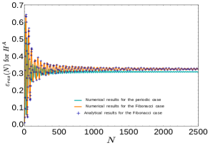
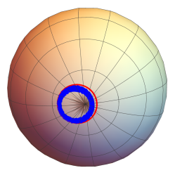
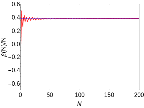
Figure 1: (a) Numerical results for the RE, $\sum_{k}[\bra{\psi_{k}(N)}H_{k}^{A}\ket{\psi_{k}(N)}-$ $e^{g}_{k}(0)]/L$, vs $N$. The cyan curve shows the RE for perfectly periodic driving with the protocol given in Eq. (2). The orange curve show the RE when $\ket{\psi_{k}(N)}$ is generated by the Fibonacci sequence. The plus signs indicate the approximate analytical results for the Fibonacci case using the unitary evolution in Eq. (7), and they show an excellent fit to the numerical results. (b) Trajectory $\{\theta_{k}(N),\phi_{k}(N)\}$ of the state $\ket{\psi_{k}(N)}$ in Eq. (13) on the Bloch sphere as a function of $N$ up to $N=1000$ for a particular momentum mode $k=159\pi/200$. In (a) and (b), we have chosen $L=500$, $\omega=500$, and $h_{A}=1$ and $h_{B}=10$ in Eq. (2). The trajectory (in red) for the periodic dynamics (with the protocol in Eq. (2)) forms a circle on the Bloch sphere. The trajectory for the Fibonacci driven sequence (in blue) fluctuates within the area bounded by two nearby and concentric circles lying on the Bloch sphere. (c) The figure shows that $\beta(N)/N$ quickly reaches a steady state value, equal to $0.382$ shown by the blue line, as $N$ becomes large. The inset shows that $\delta(N)/N$ keeps fluctuating with the same amplitude even when $N$ becomes large.

Before evaluating a local observable, we examine the dynamics of the time evolved state $\ket{\psi_{k}(N)}$ vs $N$ on the Bloch sphere for each $k$ mode. This state is numerically generated by acting with the Fibonacci evolution operator $U_{k}(N)$ on the initial state $\ket{\psi_{k}(0)}$ to yield

$$\ket{\psi_{k}(N)}=U_{k}(N)\ket{\psi_{k}(0)}=\begin{bmatrix}\cos\left(\theta_{k}(N)/2\right)\\ \sin\left(\theta_{k}(N)/2\right)e^{i\phi_{k}(N)}\\ \end{bmatrix}.$$ (11)

In Fig. 1, we show the trajectory of $(\theta_{k}(N),\phi_{k}(N))$ for a particular $k$ mode on the Bloch sphere as it evolves with increasing $N$. We note that in contrast to the trajectory for the case of periodic driving shown by the red circle, the trajectory of the points for the Fibonacci driving fluctuates but always lies in the area bounded by two nearby and concentric circles lying on the Bloch sphere. This behavior can be understood by noting that although $\beta(N)/N$ quickly reaches a steady state value equal to $1-1/G\simeq 0.382$ as $N$ becomes large, $\delta(N)/N$ continues to fluctuate even for very large $N$; see Fig. 1 and its inset. The persistent fluctuations in $\delta(N)/N$ prevents the trajectory from collapsing on to a single circle such as in the periodic case. The spread of the trajectory on the Bloch sphere is $k$-dependent and is directly related to the amount of fluctuations of $\delta(N)/N$. Reference SM provides an analytical derivation of $\beta(N)/N$ and the spread in $\delta(N)/N$ which is found to lie between $1-1/G$ and $-1/G\simeq-0.618$.

Given the trajectory of the Fibonacci time-evolved state on the Bloch sphere, we are now ready to study whether the system attains a steady state asymptotically. To this end, we calculate the RE in analogy with that of a perfectly periodic situation where the RE is given by the expectation value of the time-independent Hamiltonian $H_{k}(N)=H_{k}^{A}$ summed over all momenta modes. For the case of Fibonacci driving, we find that the Hamiltonian is $N$ dependent and is given by

$$H_{k}(N)~{}=~{}\left[\gamma(N)-1\right]H_{k}^{A}~{}+~{}\left[2-\gamma(N)\right]H_{k}^{B}.$$ (12)

Since $\gamma(N)$ is equal to either 1 or 2, $H_{k}(N)$ can either be $H_{k}^{A}$ or $H_{k}^{B}$ for each $N$. Then the RE is evaluated as $\varepsilon^{Fib}_{res}(N)=(1/L)\sum_{k}\left[\langle\psi_{k}(N)\rvert H_{k}(N)\lvert\psi_{k}(N)\rangle-e_{k}^{g}(0)\right]$. Using the high frequency approximation (7), the state after $N$ stroboscopic intervals can be written as

$$\lvert\psi_{k}(N)\rangle=e^{-iNTH_{k}^{Fib}(N)}\ket{\psi_{k}(0)}.$$ (13)

Using the basis of eigenstates of $H_{k}^{Fib}(N)$, we can evaluate the RE in the high frequency limit for a thermodynamically large system with $L\to\infty$,

$$\varepsilon_{res}^{Fib}(N) = \int\frac{dk}{2\pi}\{\lvert c_{k}^{+}(N)\rvert^{2}H_{k}^{++}(N)+\lvert c_{k}^{-}(N)\rvert^{2}H_{k}^{--}(N)$$ (14)

$$+~{}(e^{iNT[\mu_{k}^{+}(N)-\mu_{k}^{-}(N)]}c_{k}^{+*}(N)c_{k}^{-}(N)H_{k}^{+-}(N)$$

$$~{}~{}~{}~{}+~{}\text{c.c.})~{}-~{}e_{k}^{g}(0)\},$$

where $c_{k}^{\pm}(N)=\langle f_{k}^{\pm}(N)\rvert\psi_{k}(0)\rangle$, and $\ket{f_{k}^{\pm}}(N)$ are the eigenstates with eigenvalues $\mu_{k}^{\pm}(N)=\sqrt{a_{1}^{2}+a_{2}^{2}+a_{3}^{2}}$ of the Hamiltonian $H_{k}^{Fib}(N)$. The matrix elements of $H_{k}(N)$ in this basis are given by

$$H_{k}^{\pm\pm}(N)=\bra{f_{k}^{\pm}(N)}H_{k}(N)\ket{f_{k}^{\pm}(N)}.$$ (15)

In the limit of large $N$, the off-diagonal terms containing $H_{k}^{+-}(N)$ and its complex conjugate in Eq. (14) oscillate rapidly and vanish on integrating over all the $k$ modes due to the Riemann-Lebesgue lemma, giving the steady state expression

$$\varepsilon^{Fib}_{res}$$ (16)

$$= \int\frac{dk}{2\pi}~{}\{|c_{k}^{+}(N)|^{2}H_{k}^{++}(N)+|c_{k}^{-}(N)|^{2}H_{k}^{--}(N)-e_{k}^{g}(0)\}$$

$$= \left[\gamma(N)-1\right]\langle H^{A}\rangle~{}+~{}\left[2-\gamma(N)\right]\langle H^{B}\rangle,$$

where we have used Eqs. (12) and (15) and the terms $\langle H^{A/B}\rangle$ are given by,

$$\langle H^{A/B}\rangle=\int\frac{dk}{2\pi}\left\{\sum_{j=\pm}|c_{k}^{j}(N)|^{2}\bra{f_{k}^{j}(N)}H_{k}^{A/B}\ket{f_{k}^{j}(N)}\right\}.$$ (17)

The quantities $\langle H^{A/B}\rangle$ can be obtained from the expectation values of $H^{A/B}$,

$$\langle H^{A/B}(N)\rangle=\int\frac{dk}{2\pi}\left\{\bra{\psi_{k}(N)}H_{k}^{A/B}\ket{\psi_{k}(N)}-e_{k}^{g}(0)\right\}.$$ (18)

In taking the limit of large $N$, we drop the highly oscillating off-diagonal terms as they vanish upon integration over all the momentum modes in the thermodynamic limit. Although the diagonal terms depend on $N$ through the basis vectors $\ket{f_{k}^{\pm}(N)}$, the quantities $\langle H^{A}\rangle$ and $\langle H^{B}\rangle$ reach a steady state for a thermodynamically large system in the limit of large $N$ as shown in Fig. 2. The system reaches a steady state because the contributions of the fluctuating $\delta(N)/N$ terms to $\langle H^{A/B}\rangle$ vanish up on integration over the $k$ modes. Moreover, the steady state value of $\langle H^{A/B}\rangle$ also depends on $\beta(N)/N$ which, after some initial transients, settles to a value equal to $1-1/G$ and becomes independent of time.

Here, we would like to remark about the role of the $N$-dependence of $\gamma(N)$ in Eq. (16). In the case of a perfectly periodic driving, the steady state attains a constant value only when the system is observed at asymptotic stroboscopic instants $N$. There could of course be micromotion present in the system within a stroboscopic interval. If the system is observed at such intermediate times, it may not appear as steady. Similarly, in the case of the Thue-Morse sequence nandy17 , the steady state emerges only when it is observed at geometric intervals of $2^{N}$ and not at stroboscopic intervals $N$. In our case, the steady state state only attains a constant value when it is observed at the $A$ or $B$ stroboscopic instants of the Fibonacci sequence. Of course, it quasiperiodically oscillates between two different constant values (see Fig. 2) if the system is instead observed at each stroboscopic instant $N$. But, if we observe the system at the time instances $A$ or $B$, then the corresponding steady state has only one constant value.

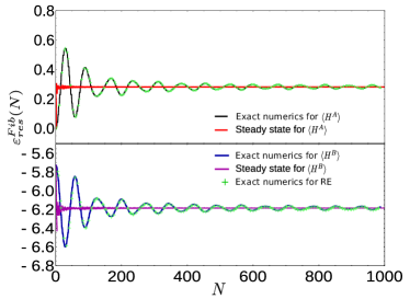
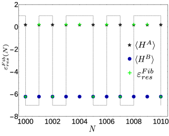
Figure 2: (a) $\langle H^{A}\rangle$ and $\langle H^{B}\rangle$ in Eq. (17) plotted vs $N$ for a Fibonacci protocol driven system with $h_{A}=1$, $h_{B}=10$, $\omega=500$, and $L=500$. The solid black (blue) lines show the numerically obtained results for $\langle H^{A}\rangle$ ($\langle H^{B}\rangle$), while the red (magenta) lines are the corresponding analytical steady state values. The green plus signed markers show how the RE (given in Eq. (16)) is supported on the two quantities $\langle H^{A}\rangle$ and $\langle H^{B}\rangle$. (b) This zoomed section of (a) focuses on the part between $N=1000$ and $1010$. The black (blue) markers indicate the values of the $\langle H^{A}\rangle$($\langle H^{B}\rangle$). Following the green markers placed on top of the black (blue) markers, we observe that the steady state RE has support only on the upper (lower) branch when the system is viewed along the $A$ ($B$) sequence in the Fibonacci series shown by the gray dashed line.

In summary, we have studied the behavior of a transverse Ising chain subjected to a Fibonacci driving protocol. For periodic driving, the evolution of each momentum mode on the Bloch sphere observed for a sufficiently long duration lies on a circle. In contrast, for the case of Fibonacci driving, we find in the high frequency limit that the evolving points lie within a small area bounded by two concentric circles on the surface of the sphere; we have provided an explanation for this in terms of small but persistent fluctuations in the evolution operator. (It turns out that the axis of rotation of the circle changes after an astronomically large number of drives. Namely, the direction of the axis changes by $\epsilon$ after a number of drives of the order of $G^{\epsilon c/T^{2}}$, where $c$ is a number of order 1. For some fixed values of $\epsilon$ and $c$, this is an enormously large number if $T$ is very small. Thus a change in the axis and therefore in the steady state would not be discernible within experimental time scales. This analysis is presented in Ref. SM ). Thus we have the interesting result that a thermodynamically large many-body system viewed stroboscopically reaches a different Fibonacci NESS and does not heat up to an ITE in the limit of large $N$. Rather, when viewed after stroboscopic intervals $N$, the RE oscillates between two steady state values of the REs of the two Hamiltonians $H^{A}$ and $H^{B}$. These oscillations are quasiperiodic and exactly follow the Fibonacci sequence. Whenever the sequence hits $A$ or $B$, the RE of the system follows the steady state RE calculated using $H^{A}$ or $H^{B}$. Thus, if the residual energy of the system is measured not after every stroboscopic interval, but either along the $A$’s in the Fibonacci sequence or along the $B$’s, it would appear that the steady state value of the RE is equal to the steady residual energy measured with respect to either $H^{A}$ or $H^{B}$, respectively. It is worth noting that the system has two accessible steady states between which the ones associated with $\langle H^{B}\rangle$ release energy and have a negative RE (see Fig. 2) compared to the initial state. This negative value of the RE occurs due to a greater population of those energy levels of $H^{B}$ which have lower energy than that of the initial ground state. This negative value can be tuned by varying the frequency $\omega$ and the field $h_{B}$ with respect to $h_{A}$. In comparison, the RE in the perfectly periodic situation is always semi-positive. To conclude, in spite of the quasiperiodic nature of the driving, it is remarkable that the local properties of the system in the long-time limit manage to synchronize with the quasiperiodic drive and can eventually be described by a different nonequilibrium statistical ensemble.

We establish these findings by analytically deriving an effective Hamiltonian $H_{k}^{Fib}(N)$, which is $N$-dependent unlike the periodic Floquet scenario and can nearly exactly simulate the dynamics of the system in the high frequency limit (see Fig. 1). The time-dependent spectrum of $H_{k}^{Fib}(N)$ can effectively provide a microscopic understanding of the nature of evolution towards a steady state as $N$ becomes large.

We would like to conclude by highlighting that our work interestingly shows the emergence of a steady state behavior albeit only at high frequencies. The emergence of such a steady state and its form (namely, an annular spread of the eigenstates on the Bloch sphere) are not a priori obvious. The uniqueness of the steady state lies in the fact that when the system is observed perfectly periodically, the steady state value oscillates quasiperiodically following the Fibonacci sequence whereas, if it is observed at Fibonacci instances, the system oscillates periodically between two constant values. Furthermore, this emergent behavior is well explained through an analytical framework devised using the high frequency approximation which is in complete agreement with numerical simulations. The analytical results allow us to explore the behavior of the system in the large $N$ limit, where numerical errors due to matrix multiplications eventually creep in. We note that if the frequency is not high, no such steady state exists, and the system can exhibit a rich variety of long-time behaviors depending on the values of the driving parameters nandy18 . The role of interactions and disorder and the eventual heating up to an ITE has been investigated in Ref. dumitrescu18 .

As long as the driving sequence is of the Fibonacci type, the fact that the system eventually reaches a steady state is not restricted to the square pulse nature of the driving protocol, though the steady state value of the RE may depend on the strength of the driving involved. The analytic evaluation of the RE assumes a knowledge of the binary non-commuting unitary evolution operators over a complete stroboscopic period whose generators are Jordan-Wigner integrable and are devoid of local disorder. Thus, the same results are expected to hold for higher-dimensional systems as well. We note that the binary aperiodic situation comprising a $\delta$-function kicking protocol has already been experimentally realized for a single rotor sarkar17 ; similar experimental studies for our quasiperiodically driven situation are indeed possible.

We thank Sourav Nandy and Arnab Sen for many stimulating discussions. A.D. acknowledges SERB, DST, India and D.S. thanks DST, India for Project No. SR/S2/JCB-44/2010 for financial support.

I The model and the steady state for periodic driving

We consider the one-dimensional transverse field Ising model as an example of a Jordan-Wigner integrable system [S1-S4] This is described by the Hamiltonian

$$H(t)~{}=~{}-~{}\sum_{n=1}^{L}~{}\tau_{n}^{x}\tau_{n+1}^{x}~{}-~{}h(t)~{}\sum_{n=1}^{L}~{}\tau_{n}^{z},$$ (S1)

where $h$ is the time-dependent transverse field and $\tau_{n}^{a}$ $\{a=x,y,z\}$ are the Pauli spin matrices at the $n^{th}$ site. Following a Jordan-Wigner transformation from spin-1/2’s to spinless fermion operators at each site, the Hamiltonian gets decoupled into two-level systems for pairs of Fourier modes with momenta $\pm k$ (where $k$ lies in the range $[0,\pi]$), such that

$$H(t) = \int_{0}^{\pi}\frac{dk}{2\pi}~{}\left(\begin{array}[]{cc}c_{k}^{\dagger}&c_{-k}\end{array}\right)~{}H_{k}(t)\left(\begin{array}[]{c}c_{k}\\ c_{-k}^{\dagger}\end{array}\right),$$ (S5)

$$H_{k}(t) = [h(t)~{}-~{}\cos k]~{}\sigma_{z}~{}+~{}\sin k~{}\sigma_{x},$$ (S6)

where the $\sigma$’s are again Pauli matrices. Here we have applied antiperiodic boundary conditions for even $L$ so that $k=2m\pi/L$ with $m=-(L-1)/2,\cdots,-1/2,1/2,\cdots,(L-1)/2$.

We first consider perfectly periodic driving with $H_{k}(t+\tau)=H_{k}(t)$, where the time period is $\tau=2T$, with a square pulse driving protocol of the form

$$H_{k}(t)~{}=~{}\begin{cases}H_{k}^{A}\hskip 8.53581pt\text{for}\hskip 8.53581pt0~{}\leq~{}t~{}<~{}T,\\ H_{k}^{B}\hskip 8.53581pt\text{for}\hskip 8.53581ptT~{}\leq~{}t~{}<~{}2T,\end{cases}$$ (S7)

where $H_{k}^{A}$ and $H_{k}^{B}$ are the momentum space Hamiltonian given in Eq. (S6) with transverse fields $h_{A}$ and $h_{B}$, respectively. For such a periodic protocol the system reaches a periodic steady state and the residual energy density (RE) reaches a steady state value russomanno12 (see the cyan curve in Fig. 1(a) of the main text). We recall here that the RE is defined as the difference between the energy density of the time evolved state determined by the expectation value of the instantaneous Hamiltonian and the energy density of the initial state of the system. Namely, $\varepsilon_{res}(t)\equiv(1/L)\sum_{k}[e_{k}(t)-e_{k}^{g}(0)]$, where $e_{k}(t)=\langle\psi_{k}(t)\rvert H_{k}(t)\lvert\psi_{k}(t)\rangle$ and $e_{k}^{g}(0)=\langle\psi_{k}(0)\rvert H_{k}(0)\lvert\psi_{k}(0)\rangle$, $\ket{\psi_{k}(t)}$ is the time evolved state starting from the initial state $\ket{\psi_{k}(0)}$, and $H_{k}(0)$ and $H_{k}(t)$ are the initial and instantaneous Hamiltonians of the system respectively.

We choose the ground state of the Hamiltonian $H_{k}^{A}$ to be the initial state $|\psi_{k}(0)\rangle$ for each $k$ mode. Using the Floquet formalism, we can define a Floquet evolution operator $\mathcal{F}_{k}(\tau)=\mathcal{T}$ $\exp\left[-i\int_{0}^{\tau}H_{k}(t)dt\right]$, where $\mathcal{T}$ denotes time ordering. We now recall that the solutions of the Schrödinger equation for a time periodic Hamiltonian can be written as $\lvert\psi_{k}^{j}(t)\rangle=\exp(-i\epsilon_{k}^{j}\tau)\lvert\phi_{k}^{j}(t)\rangle$, where the states $\lvert\phi_{k}^{j}(t)\rangle$ satisfying the condition $\lvert\phi_{k}^{j}(t+\tau)\rangle=\lvert\phi_{k}^{j}(t)\rangle$ are called Floquet modes and the real quantities $\epsilon_{k}^{j}$ are known as Floquet quasienergies. For our square pulse protocol, the Floquet evolution operator in a single interval of $\tau$ can be written in the form

$$\mathcal{F}_{k}(\tau)~{}=~{}e^{-iTH_{k}^{B}}~{}e^{-iTH_{k}^{A}},$$ (S8)

and is generated by two piecewise constant Hamiltonians $H_{k}^{A}$ and $H_{k}^{B}$. For a periodic drive of a system reducible to decoupled two-level systems, Eq. (S8) can be calculated analytically. We now note that in the high-frequency limit (i.e., small $\tau$), Eq. (S8) can be approximated, using the Baker-Campbell-Hausdorff (BCH) formula $\exp(C)\exp(D)=\exp(C+D+(1/2)[C,D]+\cdots)$, by

$$\mathcal{F}_{k}(\tau)~{}=~{}\exp[-i(\tau/2)(H_{k}^{A}+H_{k}^{B}+\tau\Delta_{h}\sin k~{}\sigma_{y})],$$ (S9)

where $\Delta_{h}=(h_{B}-h_{A})/2$. We note that this truncation scheme is similar to the Magnus expansion.

To establish that a periodically steady behavior [S5,S6] exists for our Jordan-Wigner integrable system under the periodic protocol in Eq. (S7), we will now evaluate the RE of the system. For the periodically driven case in Eq. (S7) with $H_{k}(N\tau)=H_{k}(0)=H_{k}^{A}$, we have, after a time $t=N\tau$ made up of $N$ stroboscopic intervals, $\lvert\psi_{k}(N)\rangle=\sum_{j=\pm}r_{k}^{j}e^{-i\epsilon_{k}^{j}N\tau}\lvert\phi_{k}^{j}(t)\rangle$, where $r_{k}^{\pm}=\langle\phi_{k}^{\pm}\rvert\psi_{k}(0)\rangle$. In the thermodynamic limit $L\to\infty$, we obtain

$$\varepsilon_{res}(N)~{}=~{}\int\frac{dk}{2\pi}~{}\biggl{[}~{}\sum_{\alpha=\pm}~{}|r_{k}^{\alpha}|^{2}\langle\phi_{k}^{\alpha}\rvert H_{k}^{A}\lvert\phi_{k}^{\alpha}\rangle-e_{k}^{g}(0)~{}+~{}\sum_{\begin{subarray}{c}\alpha,\beta=\pm\\ \alpha\neq\beta\end{subarray}}r_{k}^{\alpha\ast}r_{k}^{\beta}e^{i(\epsilon_{k}^{\alpha}-\epsilon_{k}^{\beta})N\tau}\langle\phi_{k}^{\alpha}\rvert H_{k}^{A}\lvert\phi_{k}^{\beta}\rangle~{}\biggr{]}.$$ (S10)

In the limit $N\to\infty$, the rapidly oscillating off-diagonal terms in Eq. (S10) will vanish upon integration over all $k$ modes leading to a steady state expression for $\varepsilon_{res}(N)$ russomanno12 (see the cyan curve in Fig. 1 (a) of the main text).

II Calculation of evolution operator $U(N)$ for Fibonacci driving

We now present a detailed calculation of the stroboscopic evolution operator $U(N)$ for a Fibonacci sequence of driving generated by two type of pulses $A$ and $B$ with Hamiltonians $H^{A}$ and $H^{B}$, respectively. (All the discussion here will refer to a particular $k$ mode, and we will not show the label $k$ explicitly). Reading from left (earliest time) to right (latest time), the Fibonacci sequence is given by

$$ABAABABAABAABABAABABA\cdots.$$ (S11)

The stroboscopic time evolution operators after the first few stroboscopic intervals $N$ are given by

$$U(N=1) = e^{-iH^{A}T}\equiv e^{A},$$ (S12)

$$U(N=2) = e^{-iH^{B}T}e^{-iH^{A}T}\equiv e^{B}e^{A}\approx e^{B+A+\frac{1}{2}[B,A]},$$ (S13)

$$U(N=3) = e^{A}U(N=2)\approx e^{A+B+A+\frac{1}{2}[B,A]+\frac{1}{2}[A,B]},$$ (S14)

$$U(N=4) = e^{A}U(N=3)\approx e^{A+A+B+A+\frac{1}{2}[B,A]+\frac{1}{2}[A,B]+\frac{1}{2}[A,B]},$$ (S15)

$$U(N=5) = e^{B}U(N=4)\approx e^{B+A+A+B+A+\frac{1}{2}[B,A]+\frac{1}{2}[A,B]+\frac{1}{2}[A,B]+\frac{3}{2}[B,A]},$$ (S16)

$$U(N=6) = e^{A}U(N=5)\approx e^{A+B+A+A+B+A+\frac{1}{2}[B,A]+\frac{1}{2}[A,B]+\frac{1}{2}[A,B]+\frac{3}{2}[B,A]+[A,B]},$$ (S17)

and so on. In Eqs. (S13) to (S17), we have used the BCH formula and considered only terms to leading order in the time period $T$ (i.e., up to $T^{2}$ to keep only the first order commutator of $A$ and $B$); this is valid for small values of $T$.

Table 1: Stroboscopic Fibonacci sequence at Fibonacci steps ($N=F_{n}$)

Fibonacci sequence of $A$’s and $B$’s	Total number of stroboscopic intervals $N$	Number of $A$’s ($X$) and $B$’s ($Y$)
A	1 ($F_{2}$)	$X=1$ $(F_{1}),Y=0$ $(F_{0})$
AB	2 ($F_{3}$)	$X=1$ $(F_{2}),Y=1$ $(F_{1})$
ABA	3 ($F_{4}$)	$X=2$ $(F_{3}),Y=1$ $(F_{2})$
ABAAB	5 ($F_{5}$)	$X=3$ $(F_{4}),Y=2$ $(F_{3})$
ABAABABA	8 ($F_{6}$)	$X=5$ $(F_{5}),Y=3$ $(F_{4})$
ABAABABAABAAB	13 ($F_{7}$)	$X=8$ $(F_{6}),Y=5$ $(F_{5})$
ABAABABAABAABABAABABA	21 ($F_{8}$)	$X=13$ $(F_{7}),Y=8$ $(F_{6})$
⋮	⋮	⋮

To determine the evolution operator $U(N)$ for arbitrary $N$, let us first consider the case where $N$ is equal to a Fibonacci number $F_{n}$, i.e., at the Fibonacci steps as shown in Table 1. In the Fibonacci sequence with $N=F_{n}$, the number of $A$’s and $B$’s present are given by $F_{n-1}$ and $F_{n-2}$, respectively. This follows from the definition of the Fibonacci numbers

$$F_{n+1}~{}=~{}F_{n}~{}+~{}F_{n-1},$$ (S18)

with the first few Fibonacci numbers being given by $F_{0}=0$, $F_{1}=1$, $F_{2}=1$, $F_{3}=2$, and $F_{4}=3$. Let $G=(\sqrt{5}+1)/2\simeq 1.618$ denote the Golden ratio; we will repeatedly use the identity $G^{2}=G+1$ below. We can show from Eq. (S18) and the values of $F_{0}$ and $F_{1}$ that

$$F_{n}~{}=~{}\frac{1}{\sqrt{5}}~{}\left[G^{n}~{}-~{}\left(-\frac{1}{G}\right)^{n}\right].$$ (S19)

For large $n$, we have $F_{n}\simeq G^{n}/\sqrt{5}$ and therefore $F_{n}/F_{n-1}\approx G$. For large values of $N=F_{n}$, the number of $A$’s and $B$’s present in the expression for $U(N)$ are therefore given by

$$X~{}\approx~{}\frac{NG}{1+G}\hskip 8.5359pt\text{and}\hskip 8.5359ptY~{}\approx~{}\frac{N}{1+G},$$ (S20)

respectively, such that $X+Y=N$ and $X/Y\approx G$.

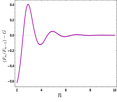
Figure S1: Figure showing that the ratio $F_{n}/F_{n-1}$ approaches $G$ very quickly as $n$ increases.

To calculate the number of $A$’s and $B$’s for an arbitrary value of $N$, let us consider the function

$$\gamma(m)=\lfloor(m+1)G\rfloor-\lfloor mG\rfloor,$$ (S21)

where $\lfloor x\rfloor$ denotes the largest integer $\leq x$. The function $\gamma(m)$ is equal to either 1 or 2 for any positive integer $m$. Therefore, the function $\gamma(m)-1$ is a Boolean function; interestingly, it generates the Fibonacci sequence of $1$’s and $0$’s as

$$101101011011010110101\cdots$$ (S22)

for positive integer values of $m$. If we take 1 to correspond to $A$ and 0 to correspond to $B$, the above sequence is exactly the same as the sequence given in Eq. (S11) and is represented by the function

$$S(N)=\left[\gamma(N)-1\right]A+\left[2-\gamma(N)\right]B.$$ (S23)

For a particular stroboscopic instant $N$, if the function $\gamma(N)$ is 1 (2), it implies that a $B$-pulse ($A$-pulse) is present. Hence, the total number of $B$ pulses in the sequence up to $N$ stroboscopic intervals is given by

$$\beta(N)=\sum_{m=1}^{N}\left\{2-\gamma(m)\right\},$$ (S24)

and the total number of $A$ pulses in the sequence is given by

$$\alpha(N)=\sum_{m=1}^{N}\left\{\gamma(m)-1\right\}=N-\beta(N).$$ (S25)

Now, in order to calculate $U(N)$ in Eqs. (S13) to (S17), it is necessary to count the number of commutators $[A,B]$ or $[B,A]$. It is easy to see that depending on whether the pulse $A$ or $B$ is present at the $m^{th}$ stroboscopic instant (where $m\leq N$), the number of commutators $[A,B]$ or $[B,A]$ is only given by the number of $B$ or $A$ pulses present in the sequence up to the $(m-1)^{th}$ stroboscopic instant. The function $\lfloor(mG)/(1+G)\rfloor$ gives the number of $A$ pulses present in the sequence before the $m^{th}$ $B$ pulse and $\lfloor(m)/(1+G)\rfloor$ gives the number of $B$ pulses present before the $m^{th}$ $A$ pulse, as illustrated in Table 2.

Table 2: Illustration of the numbers of $[A,B]$’s and $[B,A]$’s.

$N=$	1	2	3	4	5	6	7	8	9	10	11	12	13	14	15	16	17	18	19	20	21	$\cdots$
$S(N)=$	A	B	A	A	B	A	B	A	A	B	A	A	B	A	B	A	A	B	A	B	A	$\cdots$
$\big{\lfloor}\frac{m}{1+G}\big{\rfloor}=$	0	0	1	1	1	2	2	3	3	3	4	4	4	5	5	6	6	6	7	7	8	$\cdots$
$\big{\lfloor}\frac{mG}{1+G}\big{\rfloor}=$	0	1	1	2	3	3	4	4	5	6	6	7	8	8	9	9	10	11	11	12	12	$\cdots$

Now, we can calculate the number of commutators $[A,B]$ present in the evolution operators $U(N)$; this is given by

$$\delta(N)=\sum_{m=1}^{N}\left[\left\{\gamma(m)-1\right\}\Bigg{\lfloor}\frac{m}{1+G}\Bigg{\rfloor}-\left\{2-\gamma(m)\right\}\Bigg{\lfloor}\frac{mG}{1+G}\Bigg{\rfloor}\right],$$ (S26)

where the first term comes from counting all the commutators $[A,B]$ due to the positions of $A$ pulses and and the second term comes from counting all the commutators $[B,A]$ due to the positions of $B$ pulses. Using the relation $\lfloor m/(1+G)\rfloor+\lfloor mG/(1+G)\rfloor=m-1$, one can easily simplify the above expression as

$$\delta(N)=\sum_{m=1}^{N}\left\{(\gamma(m)-1)(m-1)-\Bigg{\lfloor}\frac{mG}{1+G}\Bigg{\rfloor}\right\}.$$ (S27)

Using Eqs. (S24), (S25) and (S27), the stroboscopic evolution operator $U(N)$ for an arbitrary instant $N$ in the high frequency approximation is thus found to be

$$U(N) = \exp\left\{\alpha(N)A+\beta(N)B+\frac{\delta(N)}{2}[A,B]\right\}$$ (S28)

$$= \exp\left\{-iT\alpha(N)H^{A}-iT\beta(N)H^{B}-\frac{T^{2}\delta(N)}{2}[H^{A},H^{B}]\right\}.$$ (S29)

III Calculation of the spread in the values of $\delta(N)/N$

We will now present more explicit expressions for $\alpha(N),~{}\beta(N)$ and $\delta(N)$ as functions of $N$; this will enable us to precisely calculate the spread in the values of $\delta(N)/N$. We consider the expression in Eq. (S28) which we get after $N$ stroboscopic drives. Given two matrices $U(N)$ and $U(M)$, we find that

$$U(P)~{}\equiv~{}U(M)~{}U(N)$$ (S30)

will have coefficients $\alpha(P),~{}\beta(P),~{}\delta(P)$ given by

$$\alpha(P) = \alpha(M)~{}+~{}\alpha(N),~{}~{}~{}\beta(P)~{}=~{}\beta(M)~{}+~{}\beta(N),$$

$${\rm and}~{}~{}~{}\delta(P) = \delta(M)~{}+~{}\delta(N)~{}+~{}\alpha(M)\beta(N)~{}-~{}\beta(M)\alpha(N),$$ (S31)

where we have used the BCH formula up to first order in the commutators.

The first few $U(N)$’s are given in Eqs. (S12) - (S17). This tells us that

$$\alpha(1) = 1,~{}~{}~{}\beta(1)~{}=~{}0,~{}~{}~{}\delta(1)~{}=~{}0,$$

$$\alpha(2) = 1,~{}~{}~{}\beta(2)~{}=~{}1,~{}~{}~{}\delta(2)~{}=~{}-1,$$

$$\alpha(3) = 2,~{}~{}~{}\beta(3)~{}=~{}1,~{}~{}~{}\delta(3)~{}=~{}0,$$

$$\alpha(4) = 3,~{}~{}~{}\beta(4)~{}=~{}1,~{}~{}~{}\delta(4)~{}=~{}1,$$ (S32)

and so on.

We now consider the case where $N=F_{n+1}$ is a Fibonacci number. Let us define

$$V_{n}~{}\equiv~{}U(F_{n+1}).$$ (S33)

We then have the recursion relation

$$V_{n}~{}=~{}V_{n-2}~{}V_{n-1}$$ (S34)

for $n\geq 2$, where $V_{0}=e^{B}$ and $V_{1}=e^{A}$. Using Eq. (S31), we find the recursion relations,

$$\alpha(F_{n+1}) = \alpha(F_{n-1})~{}+~{}\alpha(F_{n}),$$

$$\beta(F_{n+1}) = \beta(F_{n-1})~{}+~{}\beta(F_{n}),$$

$$\delta(F_{n+1}) = \delta(F_{n-1})~{}+~{}\delta(F_{n})~{}+~{}\alpha(F_{n-1})~{}\beta(F_{n})~{}-~{}\beta(F_{n-1})~{}\alpha(F_{n}).$$ (S35)

The first two equations in Eqs. (S35) along with the values of $\alpha(1),~{}\alpha(2),~{}\beta(1),~{}\beta(2)$ imply that

$$\alpha(F_{n+1})~{}=~{}F_{n}~{}~{}~{}{\rm and}~{}~{}~{}\beta(F_{n+1})~{}=~{}F_{n-1}.$$ (S36)

We then find that the last two terms in the third equation in Eqs. (S35) give

$$\alpha(F_{n-1})~{}\beta(F_{n})~{}-~{}\beta(F_{n-1})~{}\alpha(F_{n}) = F_{n-2}~{}F_{n-2}~{}-~{}F_{n-3}~{}F_{n-1}$$ (S37)

$$= -~{}(-1)^{n},$$

where we have used Eq. (S19) to derive the second equation from the first in Eq. (S37). The third equation in Eqs. (S35) then takes the form

$$\delta(F_{n+1})~{}=~{}\delta(F_{n-1})~{}+~{}\delta(F_{n})~{}-~{}(-1)^{n}.$$ (S38)

To solve this equation, we define

$$\delta^{\prime}(F_{n+1})~{}=~{}\delta(F_{n+1})~{}+~{}(-1)^{n}.$$ (S39)

Eq. (S38) then implies the recursion relation

$$\delta^{\prime}(F_{n+1})~{}=~{}\delta^{\prime}(F_{n-1})~{}+~{}\delta^{\prime}(F_{n}).$$ (S40)

Using the fact that $\delta^{\prime}(F_{2})=-1$ and $\delta^{\prime}(F_{3})=0$, we find from Eq. (S40) that

$$\delta^{\prime}(F_{n+1})~{}=~{}F_{n-2},$$ (S41)

which implies that

$$\delta(F_{n+1})~{}=~{}-~{}F_{n-2}~{}-~{}(-1)^{n}.$$ (S42)

This means that

$$\frac{\delta(N)}{N}~{}=~{}-~{}\frac{1}{G^{3}}$$ (S43)

in the limit that $N=F_{n+1}\to\infty$.

We will now study what happens if $N$ is close to but not equal to $F_{n+1}$. In particular, let us consider what happens if $N=F_{n+1}+j$, where $1\leq j\ll F_{n+1}$. We can then show that the corresponding unitary operator can be written as

$$U(N)~{}=~{}V_{m_{1}}~{}V_{m_{2}}~{}\cdots~{}V_{m_{r}}~{}V_{n},$$ (S44)

where the $r$ integers $m_{j}$ satisfy

$$1~{}\leq~{}m_{1}~{}<~{}m_{2}~{}<~{}\cdots~{}<~{}m_{r}~{}\ll~{}n.$$ (S45)

Further, Eq. (S34) implies that we can assume that no two successive integers, $m_{j}$ and $m_{j+1}$, are consecutive integers; otherwise, if $m_{j+1}=m_{j}+1$, we could use Eq. (S34) to re-write $V_{m_{j}}V_{m_{j}+1}$ as $V_{m_{j}+2}$. Hence we will assume that

$$m_{j}<m_{j+1}~{}-~{}1$$ (S46)

for all $j=1,2,\cdots,r-1$. For the operator in Eq. (S44), we see that

$$N~{}=~{}F_{n+1}~{}+~{}\sum_{j=1}^{r}~{}F_{m_{j}+1}.$$ (S47)

Eq. (S45) implies that the sum in Eq. (S47) is much smaller than $F_{n+1}$; to leading order, therefore, we still have $N\simeq F_{n+1}\simeq G^{n+1}/\sqrt{5}$.

We can now make repeated use of Eq. (S31) to compute $\delta(N)$. Since we are interested in calculating $\delta(N)/N$ in the limit $N\to\infty$, we only need to keep terms of the form $\alpha(M)\beta(N)-\beta(M)\alpha(N)$, where $M$ can take the values $F_{m_{1}+1},~{}F_{m_{2}+1},\cdots,F_{m_{r}+1}$ but $N=F_{n+1}$ is held fixed. All the other terms, where $M=F_{m_{j}+1}$ and $N=F_{m_{k}+1}$, give contributions which are much smaller than $F_{n+1}$. We then obtain

$$\delta(N)~{}=~{}-~{}F_{n-2}~{}+~{}\sum_{j=1}^{r}~{}[\alpha(F_{m_{j}+1})\beta(N)~{}-~{}\beta(F_{m_{j}+1})\alpha(N)].$$ (S48)

Next, we have

$$\alpha(F_{m_{j}+1})\beta(N)~{}-~{}\beta(F_{m_{j}+1})\alpha(N) = F_{m_{j}}F_{n-1}~{}-~{}F_{m_{j}-1}F_{n}$$ (S49)

$$\simeq \frac{G^{n+1}}{\sqrt{5}}~{}\frac{(-1)^{m_{j}+1}}{G^{m_{j}+1}},$$

to leading order. Dividing this by $N\simeq G^{n+1}/\sqrt{5}$ gives

$$\frac{\delta(N)}{N}~{}=~{}-~{}\frac{1}{G^{3}}~{}+~{}\sum_{j=1}^{r}~{}\frac{(-1)^{m_{j}+1}}{G^{m_{j}+1}}.$$ (S50)

This is one of our main equations.

The maximum and minimum values of the expression in Eq. (S50) can be found as follows. Noting that odd (even) values of $m_{j}$ make positive (negative) contributions, we see that the maximum value of $\delta(N)/N$ arises for the case $m_{1}=1,~{}m_{2}=3,~{}m_{3}=5,~{}\cdots$. (Note that this satisfies the constraint in Eq. (S46)). We then get

$$\left(\frac{\delta(N)}{N}\right)_{max} = -~{}\frac{1}{G^{3}}~{}+~{}\sum_{j=1}^{\infty}~{}\frac{1}{G^{2j}}$$ (S51)

$$= 1~{}-~{}\frac{1}{G}~{}\simeq~{}0.382.$$

(In taking the sum to go up to $j=\infty$ in the first line of Eq. (S51), we have assumed that $n$ is very large so that $m_{r}\ll n$ remains consistent even for a large value of $m_{r}$). The minimum value of $\delta(N)/N$ arises for the case $m_{1}=2,~{}m_{2}=4,~{}m_{3}=6,~{}\cdots$, which gives

$$\left(\frac{\delta(N)}{N}\right)_{min} = -~{}\frac{1}{G^{3}}~{}-~{}\sum_{j=1}^{\infty}~{}\frac{1}{G^{2j+1}}$$ (S52)

$$= -~{}\frac{1}{G}~{}\simeq~{}-~{}0.618.$$

Note that the values given in Eqs. (S51) and (S52) differ by 1.

Figure S2 shows a plot of $\delta(N)/N$ versus $N$ from 1 to $10^{6}$. We see that $\delta(N)/N$ lies between the values $1-1/G$ and $-1/G$ which are shown by horizontal red lines. The fact that a large region between these two numbers seems to be filled up suggests that a very large number of values of $\delta(N)/N$ can indeed be written in the form given in Eq. (S50).

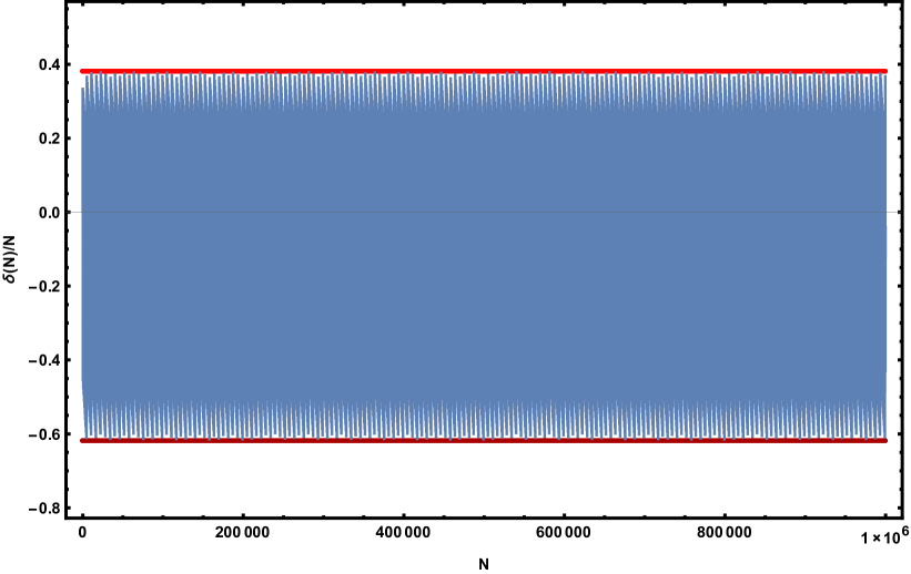
Figure S2: Plot of $\delta(N)/N$ versus the number of drives $N$. The horizontal red lines lie at the values $1-1/G\simeq 0.382$ and $-1/G\simeq-0.618$.

To summarize, we have shown that for a large number of drives, $N$, of the order of $F_{n+1}\simeq G^{n+1}/\sqrt{5}$, the unitary operator is given by

$$U(N) = \exp[\alpha(N)A~{}+~{}\beta(N)B~{}+~{}\delta(N)~{}[A,B]/2],$$

$${\rm where}~{}~{}~{}\alpha(N) \simeq \frac{G^{n}}{\sqrt{5}},~{}~{}~{}\beta(N)~{}\simeq~{}\frac{G^{n-1}}{\sqrt{5}},~{}~{}~{}{\rm and}~{}~{}~{}\delta(N)~{}\simeq~{}\gamma\frac{G^{n+1}}{\sqrt{5}},$$ (S53)

where $\gamma$ in the last equation fluctuates between the values $-1/G$ and $1-1/G$. We now consider the case where $A$ and $B$ are equal to $i$ times some linear combinations of the three Pauli matrices. We can then write Eq. (S53) in the form

$$U(N)~{}=~{}e^{i\theta_{N}{\hat{e}}_{N}\cdot{\vec{\sigma}}},$$ (S54)

where the angle $\theta_{N}$ and the unit vector $\hat{e}_{N}$ vary with $N$; we can think of $U(N)$ as performing a spin rotation by an angle $2\theta_{N}$ around the axis ${\hat{e}}_{N}$. We now assume that $[A,B]$ is much smaller than $A$ and $B$; this is true if the stroboscopic time period $T$ is small since $A$ and $B$ are proportional to $T$ implying that $[A,B]$ is proportional to $T^{2}$. We then see from Eq. (S53) that ${\hat{e}}_{N}\cdot{\vec{\sigma}}$ is almost fixed and is proportional to $i(GA+B)$ (multiplied by a normalization factor to ensure that its eigenvalues are equal to $\pm 1$), while $\theta_{N}$ varies with $n$ as $G^{n}/{\sqrt{5}}$. (There will be small fluctuations in ${\hat{e}}_{N}$ due to the term $\delta(N)~{}[A,B]/2$ as quantified in Eqs. (S51) and (S52)). Since the ratio of $G^{n}/{\sqrt{5}}$ to $2\pi$ is an irrational number, $\theta_{N}$ modulo $2\pi$ will cover the range $[0,2\pi]$ uniformly as $N$ varies. Thus the sequence of unitary matrices $U(N)$ is described by a unit vector ${\hat{e}}_{N}$ which is almost fixed (except for small fluctuations) and an angle $\theta_{N}$ which, modulo $2\pi$, takes all possible values in the range $[0,2\pi]$.

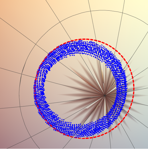
Figure S3: This figure shows the zoomed out version of Fig. 1 (b) of the main text; we see more clearly the trajectory of the points on the Bloch sphere.

We now consider what happens when a sequence of such matrices $U(N)$ acts on an initial state which is given by

$$\ket{\psi(0)}~{}=~{}\begin{bmatrix}\cos\left(\theta(0)/2\right)\\ \sin\left(\theta(0)/2\right)e^{i\phi(0)}\\ \end{bmatrix}.$$ (S55)

This state can be mapped to a point on the Bloch sphere whose Cartesian coordinates are given by $z_{0}=\cos(\theta(0)/2),~{}x_{0}=\sin(\theta(0)/2)\cos(\phi(0))$ and $y_{0}=\sin(\theta(0)/2)\sin(\phi(0))$. These coordinates define an initial unit vector ${\hat{r}}_{0}=(x(0),y(0),z(0))$. After $N$ drives, we obtain

$$\ket{\psi(N)}=U(N)\ket{\psi(0)}=\begin{bmatrix}\cos\left(\theta(N)/2\right)\\ \sin\left(\theta(N)/2\right)e^{i\phi(N)}\\ \end{bmatrix},$$ (S56)

which corresponds to a point on the Bloch sphere with coordinates $z_{N}=\cos(\theta(N)/2),~{}x_{N}=\sin(\theta(N)/2)\cos(\phi(N))$, and $y_{N}~{}=~{}\sin(\theta(N)/2)\sin(\phi(N))$ which define a unit vector ${\hat{r}}_{N}$. Given the form of $U(N)$ in Eq. (S54), where ${\hat{e}}_{N}$ is almost fixed while $\theta_{N}$ covers the range $[0,2\pi]$ as $N$ varies, we now see that the points given by ${\hat{r}}_{N}$ move on a circle which rotates around the direction ${\hat{e}}_{N}$, and the angle between ${\hat{e}}_{N}$ and ${\hat{r}}_{N}$ is almost fixed and is given by $\cos^{-1}({\hat{e}}_{N}\cdot{\hat{r}}_{0})$. This explains Fig. 3 in the main text (see also Fig. S3) where we see that all the points almost lie on a circle. More precisely, the points lie between two nearby circles which are defined by the maximum and minimum values of $\delta(N)/N$; the separation between the two circles is of the order of $[A,B]\propto T^{2}$.

IV Does the steady state remain the same up to arbitrarily large $N$ ?

In this section, we will try to understand if the steady state (in which the trajectory on the Bloch sphere is restricted to a thin ring which is centered around a particular axis) remains the same up to arbitrarily large values of $N$. We will argue that if the time period $T$ is small, the direction of the axis changes by an amount $\epsilon$ after an astronomically large number of drives given by $N_{0}\sim G^{\epsilon/T^{2}}$.

We will do our analysis for values of $N=F_{n+1}$ which are Fibonacci numbers. The time evolution operators $V_{n}=U(F_{n+1})$ then satisfy the recursion relation in Eq. (S34) for $n\geq 2$. Let us parameterize

$$V_{n}~{}=~{}e^{i\theta_{n}{\hat{e}}_{n}\cdot{\vec{\sigma}}}~{}=~{}\cos\theta_{n}~{}I_{2}~{}+~{}i\sin\theta_{n}~{}{\hat{e}}_{n}\cdot{\vec{\sigma}},$$ (S57)

where $I_{2}$ is the $2\times 2$ identity matrix, and $\theta_{n}$ can be taken to lie in the range $[0,2\pi]$. It was shown by Sutherland sutherland86 that the recursion relation in Eq. (S34) has an invariant; namely, the quantity

$$S~{}=~{}\cos^{2}\theta_{n}~{}+~{}\cos^{2}\theta_{n+1}~{}+~{}\cos^{2}\theta_{n+2}~{}-~{}2\cos\theta_{n}\cos\theta_{n+1}\cos\theta_{n+2}~{}-~{}1$$ (S58)

is independent of $n$. Further, if $\Gamma_{n,n+1}=\cos^{-1}({\hat{e}}_{n}\cdot{\hat{e}}_{n+1})$ denotes the angle between ${\hat{e}}_{n}$ and ${\hat{e}}_{n+1}$, the Sutherland invariant is equal to

$$S~{}=~{}-\sin^{2}\theta_{n}~{}\sin^{2}\theta_{n+1}~{}\sin^{2}\Gamma_{n,n+1}.$$ (S59)

We now note that in the expressions

$$V_{0}~{}=~{}e^{B}~{}~{}~{}{\rm and}~{}~{}~{}V_{1}=e^{A},$$ (S60)

$A=-iH^{A}T$ and $B=-iH^{B}T$ are both of order $T$. We can write $H^{A}={\vec{a}}\cdot{\vec{\sigma}}$ and $H^{B}={\vec{b}}\cdot{\vec{\sigma}}$, where the vectors $\vec{a}$ and $\vec{b}$ and therefore the angle between them are all of order 1. Looking at the Sutherland invariant $S$ in Eq. (S59) for $n=1$, we then see that $\sin\theta_{1}$ and $\sin\theta_{2}$ are of order $T$ while $\sin\Gamma_{n,n+1}$ is of order 1. Hence $S$ is of order $T^{4}$.

We now consider what happens if we use the recursion relation in Eq. (S34) many times. We found above that $\theta_{n}$ varies as $G^{n}$ modulo $2\pi$ for large $n$ and is therefore generally of order 1; hence $\sin\theta_{n}$ and $\sin\theta_{n+1}$ are also of order 1. Then the invariant in Eq. (S59) implies that $\sin^{2}\Gamma_{n,n+1}$ is of order $T^{4}$; hence the angle $\Gamma_{n,n+1}$ between ${\hat{e}}_{n}$ and ${\hat{e}}_{n+1}$ must be of order $T^{2}$. Since $T$ has been assumed to be small, this explains why ${\hat{e}}_{n}$ changes very slowly with $n$. Since ${\hat{e}}_{n}$ changes by only order $T^{2}$ when $n$ increases by 1, $n$ must increase by $\epsilon c/T^{2}$ for ${\hat{e}}_{n}$ to change by an angle $\epsilon$ (here $c$ is a number of order 1 which depends on the values of $\vec{a}$ and $\vec{b}$ appearing in $H^{A}$ and $H^{B}$). Since $N=F_{n+1}\simeq G^{n+1}/\sqrt{5}$ for large $n$, we see that $N$ must reach a value of the order of $N_{0}\sim G^{\epsilon c/T^{2}}$ before ${\hat{e}}_{n}$ (which determines the axis around which the ring in the Bloch sphere is centered) will change by order $\epsilon$. For small values of $T$, this is an astronomically large number. In our numerical calculations, we have taken $\omega=500$ so that $T=2\pi/500$. Hence $N_{0}\sim 1.618^{\epsilon c(500/2\pi)^{2}}$ which is about $10^{13}$ for $\epsilon=0.01$ and $c=1$. We thus see that the axis of rotation on the Bloch sphere can change appreciably and therefore give a different state, but this can only occur after an extremely large number of drives which would not be discernible within experimental time scales.

References

- (1)
- (2) I. Bloch, J. Dalibard, and W. Zwerger, Rev. Mod. Phys. 80, 885 (2008).
- (3) M. Lewenstein, A. Sanpera and V. Ahufinger, Ultracold Atoms in Optical Lattices (Oxford University Press, Oxford, U.K., 2012).
- (4) G. Jotzu, M. Messer, R. Desbuquois, M. Lebrat, T. Uehlinger, D. Greif, and T. Esslinger, Nature 515, 237 (2014).
- (5) M. Greiner, O. Mandel, T. W. Hansch, and I. Bloch, Nature 419, 51 (2002).
- (6) T. Kinoshita, T. Wenger, and D. S. Weiss, Nature 440, 900 (2006).
- (7) J. M. Deutsch, Phys. Rev. A 43, 2046 (1991).
- (8) M. Srednicki, Phys. Rev. E 50, 888 (1994).
- (9) M. Rigol, V. Dunjko, and M. Olshanii, Nature 452, 854 (2008).
- (10) A. Pal and D. A. Huse, Phys. Rev. B 82, 174411 (2010).
- (11) R. Nandkishore and D. A. Huse, Annual Review of Condensed Matter Physics 6, 15 (2015).
- (12) M. Rigol, V. Dunjko, V. Yurovsky, and M. Olshanii, Phys. Rev. Lett. 98, 050405 (2007).
- (13) A. C. Cassidy, C. W. Clark, and M. Rigol, Phys. Rev. Lett. 106, 140405 (2011).
- (14) J.-S. Caux and F. H. L. Essler, Phys. Rev. Lett. 110, 257203 (2013).
- (15) A. Lazarides, A. Das, and R. Moessner, Phys. Rev. Lett. 112, 150401 (2014).
- (16) M. Gring, M. Kuhnert, T. Langen, T. Kitagawa, B. Rauer, M. Schreitl, I. Mazets, D. Adu Smith, E. Demler, and J. Schmiedmayer, Science 337, 1318 (2012).
- (17) S. Trotzky, Y.-A. Chen, A. Flesch, I. P. McCulloch, U. Schollwöck, J. Eisert, and I. Bloch, Nat. Phys. 8, 325 (2012).
- (18) M. Cheneau, P. Barmettler, D. Poletti, M. Endres, P. Schauss, T. Fukuhara, C. Gross, I. Bloch, C. Kollath, and S. Kuhr, Nature 481, 484 (2012).
- (19) D. Fausti, R. I. Tobey, N. Dean, S. Kaiser, A. Dienst, M. C. Hoffmann, S. Pyon, T. Takayama, H. Takagi, A. Cavalleri, Science 331, 189 (2011).
- (20) M. C. Rechtsman, J. M. Zeuner, Y. Plotnik, Y. Lumer, D. Podolsky, F. Dreisow, S. Nolte, M. Segev, and A. Szameit, Nature 496, 196 (2013).
- (21) M. Schreiber, S. S. Hodgman, P. Bordia, H. P. Läschen, M. H. Fischer, R. Vosk, E. Altman, U. Schneider, I. Bloch, Science 349, 842 (2015).
- (22) T. Oka and H. Aoki, Phys. Rev. B 79, 081406 (2009).
- (23) T. Kitagawa, E. Berg, M. Rudner, and E. Demler, Phys. Rev. B 82, 235114 (2010).
- (24) N. H. Lindner, G. Refael, and V. Galitski, Nat. Phys. 7, 490 (2011).
- (25) M. Thakurathi, A. A. Patel, D. Sen, and A. Dutta, Phys. Rev. B 88, 155133 (2013).
- (26) J. Cayssol, B. Dóra, F. Simon, and R. Moessner, Phys. Status Solidi RRL 7, 101 (2013).
- (27) V. M. Bastidas, C. Emary, B. Regler, and T. Brandes, Phys. Rev. Lett. 108, 043003 (2012); V. M. Bastidas, C. Emary, G. Schaller, and T. Brandes, Phys. Rev. A 86, 063627 (2012).
- (28) S. Dasgupta, U. Bhattacharya, and A. Dutta, Phys. Rev. E 91, 052129 (2015).
- (29) L. Privitera and G. E. Santoro, Phys. Rev. B 93, 241406(R) (2016).
- (30) J. Zhang, P. W. Hess, A. Kyprianidis, P. Becker, A. Lee, J. Smith, G. Pagano, I.-D. Potirniche, A. C. Potter, A. Vishwanath, N. Y. Yao, and C. Monroe, Nature 543, 217 (2017).
- (31) S. Choi, J. Choi, R. Landig, G. Kucsko, H. Zhou, J. Isoya, F. Jelezko, S. Onoda, H. Sumiya, V. Khemani, C. v. Keyserlingk, N. Y. Yao, E. Demler, and M. D. Lukin, Nature 543, 221 (2017).
- (32) A. Russomanno, A. Silva, and G. E. Santoro, Phys. Rev. Lett. 109, 257201 (2012).
- (33) P. Ponte, Z. Papic, F. Huveneers, and D. A. Abanin, Phys. Rev. Lett. 114, 140401 (2015); P. Ponte, A. Chandran, Z. Papic, and D. A. Abanin, Ann. Phys. 353, 196 (2015).
- (34) V. Mukherjee, A. Dutta, and D. Sen, Phys. Rev. B 77, 214427 (2008); V. Mukherjee and A. Dutta, J. Stat. Mech. (2009) P05005.
- (35) A. Das, Phys. Rev. B 82, 172402 (2010).
- (36) L. D’Alessio and A. Polkovnikov, Ann. Phys. 333, 19 (2013).
- (37) A. Gomez-Leon and G. Platero, Phys. Rev. Lett. 110, 200403 (2013).
- (38) T. Nag, S. Roy, A. Dutta, and D. Sen, Phys. Rev. B 89, 165425 (2014).
- (39) A. Agarwala, U. Bhattacharya, A. Dutta, and D. Sen, Phys. Rev. B 93, 174301 (2016); A. Agarwala and D. Sen, Phys. Rev. B 95, 014305 (2017).
- (40) S. Sharma, A. Russomanno, G. E. Santoro, and A. Dutta, EPL 106, 67003 (2014).
- (41) A. Dutta, A. Das, and K. Sengupta, Phys. Rev. E 92, 012104 (2015).
- (42) A. Russomanno, S. Sharma, A. Dutta, and G. E. Santoro, J. Stat. Mech. (2015) P08030.
- (43) A. Russomanno, G. E. Santoro, and R. Fazio, J. Stat. Mech. (2016) 073101.
- (44) A. Sen, S. Nandy, and K. Sengupta, Phys. Rev. B 94, 214301 (2016).
- (45) M. Bukov, L. D’Alessio and A. Polkovnikov, Adv. Phys. 64, 139 (2015).
- (46) V. Gritsev and A. Polkovnikov, SciPost Phys. 2, 021 (2017).
- (47) L. D’Alessio and M. Rigol, Phys. Rev. X 4, 041048 (2014).
- (48) S. Nandy, A. Sen, and D. Sen, Phys. Rev. X 7, 031034 (2017).
- (49) U. Bhattacharya, S. Maity, U. Banik, and A. Dutta, Phys. Rev. B 97, 184308 (2018); S. Maity, U. Bhattacharya, and A. Dutta, Phys. Rev. B 98, 064305 (2018).
- (50) T. Ishii, T. Kuwahara, T. Mori, and N. Hatano, Phys. Rev. Lett. 120, 220602 (2018).
- (51) P. T. Dumitrescu, R. Vasseur, and A. C. Potter, Phys. Rev. Lett. 120, 070602 (2018).
- (52) A. Lazarides, A. Das, and R. Moessner, Phys. Rev. Lett. 115, 030402 (2015).
- (53) A. Haldar and A. Das, Ann. Phys. (Berlin) 529, 1600333 (2017).
- (54) M. Bukov and M. Heyl, Phys. Rev. B 86, 054304 (2012).
- (55) V. Khemani, A. Lazarides, R. Moessner, and S. L. Sondhi, Phys. Rev. Lett. 116, 250401 (2016).
- (56) D. V. Else, B. Bauer, and C. Nayak, Phys. Rev. Lett. 117, 090402 (2016).
- (57) A. Quelle and C. M. Smith, Phys. Rev. E 96, 052105 (2017).
- (58) E. Ott, T. M. Antonsen, Jr., and J. D. Hanson, Phys. Rev. Lett. 53, 2187 (1984).
- (59) I. Guarneri, Lett. Nuovo Cimento 40, 171 (1984).
- (60) G. Roósz, R. Juhász, and F. Iglói, Phys. Rev. B 93, 134305 (2016).
- (61) I. Martin, G. Refael, and B. Halperin, Phys. Rev. X 7, 041008 (2017).
- (62) S. Nandy, A. Sen and D. Sen, Phys. Rev. B 98, 245144 (2018).
- (63) E. Lieb, T. Schultz, and D. Mattis, Ann. Phys. 16, 407 (1961).
- (64) J. B. Kogut, Rev. Mod. Phys. 51, 659 (1979).
- (65) S. Suzuki, J. Inoue, and B. K. Chakrabarti, Quantum Ising Phases and Transitions in Transverse Ising Models, Lecture Notes in Physics Vol. 862 (Springer, Heidelberg, 2013).
- (66) A. Dutta, G. Aeppli, B. K. Chakrabarti, U. Divakaran, T. Rosenbaum, and D. Sen, Quantum Phase Transitions in Transverse Field Spin Models: From Statistical Physics to Quantum Information (Cambridge University Press, Cambridge, 2015).
- (67) Supplemental Material.
- (68) S. Sarkar, S. Paul, C. Vishwakarma, S. Kumar, G. Verma, M. Sainath, U. D. Rapol, and M. S. Santhanam, Phys. Rev. Lett. 118, 174101 (2017).
Supplemental Material on “Fibonacci steady states in a driven integrable quantum system”

References

- (1)
- (2) E. Lieb, T. Schultz, and D. Mattis, Ann. Phys. 16, 407 (1961).
- (3) J. B. Kogut, Rev. Mod. Phys. 51, 659 (1979).
- (4) S. Suzuki, J. Inoue, and B. K. Chakrabarti, Quantum Ising Phases and Transitions in Transverse Ising Models, Lecture Notes in Physics 862 (Springer, Heidelberg, 2013).
- (5) A. Dutta, G. Aeppli, B. K. Chakrabarti, U. Divakaran, T. Rosenbaum, and D. Sen, Quantum Phase Transitions in Transverse Field Spin Models: From Statistical Physics to Quantum Information (Cambridge University Press, Cambridge, 2015).
- (6) A. Russomanno, A. Silva, and G. E. Santoro, Phys. Rev. Lett. 109, 257201 (2012).
- (7) A. Lazarides, A. Das, and R. Moessner, Phys. Rev. Lett. 112, 150401 (2014).
- (8) B. Sutherland, Phys. Rev. Lett. 57, 770 (1986).