Type Ib/Ic supernovae: effect of nickel mixing on the early-time color evolution and implications for the progenitors

Abstract

We investigate the effect of mixing of radioactive nickel (⁵⁶Ni) on the early-time color evolution of Type Ib and Ic supernovae (SNe Ib/Ic) using multi-group radiation hydrodynamics simulations. We consider both helium-rich and helium-poor progenitors. Mixing of ⁵⁶Ni is parameterized using a Gaussian distribution function. We find that the early-time color evolution with a weak ⁵⁶Ni mixing is characterized by three different phases: initial rapid reddening, blueward evolution due to the delayed effect of ⁵⁶Ni heating, and redward evolution thereafter until the transition to the nebular phase. With a strong ⁵⁶Ni mixing, the second phase disappears. We compare our models with the early-time color evolution of several SNe Ib/Ic (SN 1999ex, SN 2008D, SN 2009jf, iPTF13bvn, SN 1994I, SN 2007gr, SN 2013ge, and 2017ein) and find signatures of relatively weak and strong ⁵⁶Ni mixing for SNe Ib and SNe Ic, respectively. This suggests that SNe Ib progenitors are distinct from SN Ic progenitors in terms of helium content and that ⁵⁶Ni mixing is generally stronger in the carbon-oxygen core and weaker in the helium-rich envelope. We conclude that the early-time color evolution is a powerful probe of ⁵⁶Ni mixing in SNe Ib/Ic.

1 Introduction

Type Ib and Ic supernovae (SNe Ib/Ic) and their progenitors constitute an important subject of stellar evolution theory (see Yoon, 2015, for a recent review). The majority of SNe Ib/Ic belong to a subclass of core-collapse SNe (ccSNe), having a massive star origin as implied by their strong correlation with star formation (e.g., Tsvetkov et al., 2001; van den Bergh et al., 2005; Anderson & James, 2009; Hakobyan et al., 2009; Habergham et al., 2010; Leloudas et al., 2011; Kelly & Kirshner, 2012; Sanders et al., 2012; Hakobyan et al., 2014; Anderson et al., 2015; Xiao & Eldridge, 2015; Kangas et al., 2017; Graur et al., 2017; Maund, 2018). Their event rate is relatively high, amounting to about 25 % of the ccSN rate (e.g., Smith et al., 2011; Eldridge et al., 2013; Shivvers et al., 2017). The lack of H I spectral lines implies that the progenitors have lost their hydrogen-rich envelope during the pre-SN evolution by stellar wind and/or binary interaction (e.g., Podsiadlowski et al., 1992; Woosley, 1993; Woosley et al., 1995; Wellstein & Langer, 1999; Eldridge & Tout, 2004; Meynet & Maeder, 2005; Eldridge et al., 2008; Yoon et al., 2010; Georgy et al., 2012; Yoon et al., 2017). The properties of SN Ib/Ic light curves and spectra imply relatively low ejecta masses (i.e., $M_{\mathrm{ejecta}}\simeq 1.0-4.0~{}\mathrm{M_{\odot}}$; e.g., Ensman & Woosley 1988; Shigeyama et al. 1990; Dessart et al. 2011; Drout et al. 2011; Bianco et al. 2014; Taddia et al. 2015; Lyman et al. 2016; Prentice et al. 2016; Taddia et al. 2018), in favor of the binary scenario for their progenitors (Yoon, 2015). The optically bright progenitor of the SN Ib iPTF13bvn, which has been recently identified in a pre-SN image (Cao et al., 2013; Folatelli et al., 2016), is also consistent with binary progenitor models in terms of the progenitor mass and optical brightness (Bersten et al. 2014; Eldridge et al. 2015; Kim et al. 2015; Fremling et al. 2016; McClelland & Eldridge 2016; Hirai 2017; Yoon et al. 2017; see also Yoon et al. 2012).

The exact nature of SN Ib/Ic progenitors is still a matter of debate. One outstanding question is what distinguishes type Ib from type Ic progenitors.

Supernovae Ib/Ic are distinguished by the presence or absence of He I lines. Because of this reason, SN Ic progenitors are often regarded as helium-poor stars in the literature. However, the absence of He I lines in SN Ic spectra does not necessarily serve as evidence for the deficiency of helium in SN Ic progenitors. This is because the formation of He I lines by non-thermal processes (Lucy, 1991; Swartz, 1991) is sensitively affected by the presence of radioactive ⁵⁶Ni, and hence by the degree of ⁵⁶Ni mixing in SN ejecta (Woosley & Eastman, 1997; Dessart et al., 2012). He I lines can be easily formed if ⁵⁶Ni were fully mixed in the SN ejecta but a large amount of helium ($M_{\mathrm{He}}\gtrsim 1.0~{}M_{\odot}$) could be effectively hidden in the spectra with a very weak ⁵⁶Ni mixing (Woosley & Eastman, 1997; Dessart et al., 2012; Hachinger et al., 2012). For an understanding of the nature of SN Ib/Ic progenitors, therefore, it would be very useful if the ⁵⁶Ni distribution in SN Ib/Ic ejecta could be constrained by observations.

The effects of ⁵⁶Ni mixing on SN Ib/Ic light curves and spectra have been studied by several authors (Ensman & Woosley, 1988; Shigeyama et al., 1990; Woosley & Eastman, 1997; Dessart et al., 2012; Bersten et al., 2013; Piro & Nakar, 2013; Dessart et al., 2015, 2016). It is found that some degree of ⁵⁶Ni mixing is needed not only for the efficient formation of He I lines in the spectra (Woosley & Eastman, 1997; Dessart et al., 2012) but also for explaining the overall shape of SN Ib light curves during the post-maximum phase  (Shigeyama et al., 1990). The early-time light curve is also found to be significantly affected by the ⁵⁶Ni distribution. For example, the post-breakout plateau of a short duration (a few to several days) that is commonly found in the models with a relatively weak ⁵⁶Ni mixing disappears with a strong ⁵⁶Ni mixing (Ensman & Woosley, 1988; Dessart et al., 2011, 2012; Piro & Nakar, 2013).

In addition, a larger ⁵⁶Ni content in the outermost layers would lead to a higher temperature of the SN Ib/Ic photosphere at very early times, resulting in a bluer color for a given progenitor structure (Piro & Nakar, 2013; Dessart et al., 2015) – a similar effect results for an extended progenitor (Nakar & Piro, 2014; Dessart et al., 2018). This implies that we can use this information to constrain the degree of ⁵⁶Ni mixing in SNe Ib/Ic but this possibility has not been properly explored yet. In this study, we present new multi-color light curve models of SN Ib/Ic calculated with the STELLA code and systematically investigate the effects of ⁵⁶Ni mixing on the early-time evolution of SNe Ib/Ic. We show that the early-time color evolution of SN Ib/Ic sensitively depends on the ⁵⁶Ni distribution, and can be a powerful probe of ⁵⁶Ni mixing in SN Ib/Ic.

This paper is organized as follows. In Section 2, we present our progenitor models, the numerical method, and the physical parameters adopted for SN calculations. In Section 3, we present the multi-color light curves of our models. We discuss the effect of ⁵⁶Ni mixing on the early-time color evolution in Section 4. We compare our models with several observed SNe Ib/Ic including SN 1994I, SN 1999ex, SN 2007gr, SN 2008D, SN 2009jf, iPTF13bvn, SN 2013ge and 2013ein in Section 5. We discuss the implications of our results for SNe Ib/Ic progenitors and ⁵⁶Ni mixing in Section 6. We conclude our study in Section 7.

2 Physical assumptions and numerical method

2.1 Input models

Table 1: Input model properties

Name	$M_{\mathrm{ej}}$	$R$	$M_{\mathrm{CO}}$	$M_{\mathrm{He,env}}$	$m_{\mathrm{He}}$	$M_{\mathrm{Fe}}$	$M_{\mathrm{ext}}$
	[$M_{\odot}$]	[$R_{\odot}$]	[$M_{\odot}$]	[$M_{\odot}$]	[$M_{\odot}$]	[$M_{\odot}$]	[$M_{\odot}$]
HE3.87	2.40	6.73	2.15	1.72	1.66	1.47	2.7(-5)
CO3.93	2.49	0.77	3.91	0.02	0.10	1.44	5.2(-4)
CO2.16	0.71	0.13	2.16	0.00	0.06	1.46	3.2(-4)

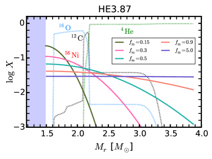
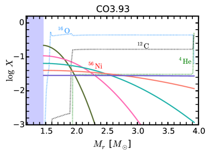
Figure 1: The chemical composition in the input models HE3.87 (upper panel) and CO3.93 (lower panel). ⁵⁶Ni profiles with $f_{\mathrm{m}}=$ 0.15, 0.3, 0.5, 0.9 and 5.0 according to equation (1) are color coded.

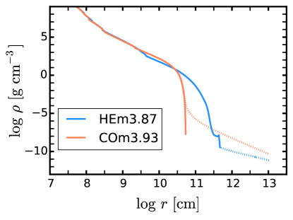
Figure 2: The density profiles of the input models HE3.87 (orange) and CO3.93 (skyblue). The solid and dotted lines give the density profiles of the progenitor models and the attached external material, respectively. See the text for details.

We consider both helium-rich and helium-poor progenitors. These models are constructed with the MESA code (Paxton et al., 2011, 2013, 2015, 2018). In Table 1, we present the properties of our progenitor models. The boundary between the helium-rich envelope and the carbon-oxygen (CO) core is defined by the condition that the mass fraction of helium in the envelope is higher than 0.1. The name starting with ‘HE’ refers to the helium-rich model, which has an integrated helium mass (i.e., $m_{\mathrm{He}}=\int X_{\mathrm{He}}dM_{r}$) of about 1.7 $M_{\odot}$, and thus is a potential SN Ib progenitor. Note that with this much helium, He I lines would be seen at early times even without non-thermal effects (Dessart et al., 2011). The name with ‘CO’ refers to the helium-poor model ($m_{\mathrm{He}}\leq 0.1M_{\odot}$), which is almost a naked CO core and can be considered a SN Ic progenitor. The number given in each model name refers to the total mass of the progenitor at the pre-SN stage.

Model HE3.87 is from the binary star model sequence Sm13p50 of Yoon et al. (2017), where the primary star of 13.0 $M_{\odot}$ starts its evolution in a 50 day orbit with a 11.7 $M_{\odot}$ companion. The calculation of this model is stopped when the central temperature reaches $10^{9}$ K in Yoon et al. (2017), and the evolution is further followed up to the pre-SN stage for the present study. Model CO2.16 has the same progenitor model and the same adopted physics as model HE3.87 but the mass-loss rate is artificially enhanced (i.e., $\dot{M}=10^{-4}~{}M_{\odot}~{}\mathrm{yr^{-1}}$) after core helium exhaustion, in order to remove the helium-rich envelope. Model CO3.93 is evolved from a pure helium star of 7.0 $M_{\odot}$ at solar metallicity, which would have a $\sim$ 20 $M_{\odot}$ main sequence progenitor. Overshooting on top of the helium-burning core is treated as a step function with an overshoot parameter of 0.1 $H_{P}$ ($H_{P}$ is the pressure scale height at the boundary of the convective core). The standard mass-loss prescription for Wolf-Rayet (WR) stars by Nugis & Lamers (2000) is adopted until core helium exhaustion and an enhanced mass-loss rate of $\dot{M}=10^{-4}~{}M_{\odot}~{}\mathrm{yr^{-1}}$ is applied thereafter until the pre-SN stage to remove the helium-rich envelope.

We assume that the mass cut in the ccSN explosion corresponds to the iron core mass $M_{\mathrm{Fe}}$, which is the innermost region above which the silicon mass fraction is higher than 0.1. We put 0.07 $M_{\odot}$ of ⁵⁶Ni by hand in the progenitor model assuming a Gaussian distribution. The degree of ⁵⁶Ni mixing is parameterized using the parameter $f_{\mathrm{m}}$, defined as

$$X_{\mathrm{Ni}}(M_{r})=A\exp\left(-\left[\frac{M_{r}-M_{\mathrm{Fe}}}{f_{\mathrm{m}}(M_{\mathrm{tot}}-M_{\mathrm{Fe}})}\right]^{2}\right)~{},$$ (1)

where $M_{r}$ is the Lagrangian mass at radius $r$, and $X_{\mathrm{M_{r}}}$ denotes the mass fraction of ⁵⁶Ni at $M_{r}$. The total mass of ⁵⁶Ni for a given $f_{\mathrm{m}}$ is determined by the normalization factor $A$. The mass fractions of the other elements are scaled to preserve a normalization of the total mass fraction to unity at each depth. We consider $f_{\mathrm{m}}=$ 0.15, 0.3, 0.5, 0.9 and 5.0. As shown in Figure 1, ⁵⁶Ni is more evenly distributed with a larger value of $f_{\mathrm{m}}$. Mixing of the other elements, which is not considered in this study, is potentially important for the early-time light curves of helium-rich models because mixing of carbon and oxygen into the helium-rich envelope can influence the opacity at the SN photosphere. For example, the importance of ionization in the opacity would be reduced with more carbon and oxygen. This effect will be addressed elsewhere.

Our progenitor models are compact ($R=6.73~{}R_{\odot}$, $0.77~{}R_{\odot}$ and $0.13~{}R_{\odot}$ for HE3.87, CO3.93 and CO2.16, respectively; Table 1), and the density decreases sharply at the outermost layers (Figure 2). This would make the shock velocity rapidly accelerate to a value close to the speed of light, while our version of the STELLA code does not include relativistic effects. To avoid numerical errors that this high shock velocity can introduce, we add a small amount of external material beyond the stellar surface (i.e., which also mimics the presence of an atmosphere or wind), so that the velocity of the shock front remains significantly below the speed of light. This mass buffer is assumed to have a wind density profile (i.e., $\rho=\dot{M}/4\pi v_{\mathrm{w}}r^{2}$) for which the standard $\beta$-law for the wind velocity $v_{\mathrm{w}}$ with $\beta=2.0$, $v_{\infty}=10~{}\mathrm{km~{}s^{-1}}$ and $\dot{M}=10^{-3}~{}M_{\odot}~{}\mathrm{yr^{-1}}$ is assumed. The maximum radius of this external material is set to $10^{13}$ cm initially (Figure 2). Because CO3.83 and CO2.16 are much more compact, the density decrease at the outer boundary is too sharp and causes too small a time step before shock breakout. Therefore we remove $\sim 10^{-6}~{}M_{\odot}$ from the original progenitor model and attach the mass buffer as shown in Figure 2. With this configuration, the ejecta velocity at the outer boundary remains lower than about $4\times 10^{4}~{}\mathrm{km~{}s^{-1}}$ in all of our SN models. Although this external structure is unrealistic, its mass is very small (i.e., $M_{\mathrm{ext}}\lesssim 5\times 10^{-4}M_{\odot}$; Table 1) and it affects the SN light curves only for a short period ($<1$ d) after shock breakout.

2.2 Supernova Models

Table 2: Properties of bolometric light curves of the SN models with $M_{\mathrm{Ni}}=0.07M_{\odot}$.

Name	$E_{\mathrm{K}}$	$L_{\mathrm{Bol,max}}$	$t_{\mathrm{Bol,{max}}}$	$\delta t_{\mathrm{Bol,-1/2}}$	$\delta t_{\mathrm{Bol,+1/2}}$	$M_{\mathrm{Bol,max}}$
	[$10^{51}$ erg]	[$10^{42}~{}\mathrm{erg~{}s^{-1}}$]	[d]	[d]	[d]	[mag]
HE3.87_fm0.15_E1.0	0.67	1.69	23.82	9.56	14.91	-16.85
HE3.87_fm0.3_E1.0	0.67	1.67	23.08	9.13	15.86	-16.84
HE3.87_fm0.5_E1.0	0.69	1.64	22.11	11.02	14.21	-16.82
HE3.87_fm0.9_E1.0	0.69	1.62	21.14	13.31	12.70	-16.81
HE3.87_fm5.0_E1.0	0.69	1.61	18.08	12.21	14.19	-16.80
HE3.87_fm0.15_E1.5	1.17	1.80	19.41	6.98	15.50	-16.92
HE3.87_fm0.3_E1.5	1.17	1.81	18.94	7.47	14.18	-16.93
HE3.87_fm0.5_E1.5	1.18	1.83	18.00	8.57	13.18	-16.94
HE3.87_fm0.9_E1.5	1.19	1.82	17.33	10.12	11.35	-16.93
HE3.87_fm5.0_E1.5	1.19	1.77	14.94	9.80	12.32	-16.90
HE3.87_fm0.15_E1.8	1.47	1.85	18.07	6.83	15.03	-16.95
HE3.87_fm0.3_E1.8	1.47	1.85	17.99	7.76	14.75	-16.95
HE3.87_fm0.5_E1.8	1.48	1.89	17.51	8.82	12.07	-16.98
HE3.87_fm0.9_E1.8	1.49	1.85	15.00	8.65	12.51	-16.95
HE3.87_fm5.0_E1.8	1.49	1.84	15.29	10.47	9.96	-16.94
CO3.93_fm0.15_E1.0	0.57	1.64	30.85	11.42	15.34	-16.82
CO3.93_fm0.3_E1.0	0.58	1.53	29.19	13.16	16.96	-16.75
CO3.93_fm0.5_E1.0	0.58	1.45	26.02	13.51	20.20	-16.69
CO3.93_fm0.9_E1.0	0.58	1.40	23.16	15.06	23.04	-16.65
CO3.93_fm5.0_E1.0	0.58	1.36	17.44	11.74	27.88	-16.62
CO3.93_fm0.15_E1.5	1.07	1.87	24.93	9.74	19.73	-16.97
CO3.93_fm0.3_E1.5	1.08	1.79	24.86	12.08	18.85	-16.91
CO3.93_fm0.5_E1.5	1.08	1.70	22.10	11.04	19.43	-16.86
CO3.93_fm0.9_E1.5	1.08	1.62	18.97	11.85	18.99	-16.81
CO3.93_fm5.0_E1.5	1.08	1.55	15.32	10.25	21.27	-16.76
CO3.93_fm0.15_E1.8	1.37	1.99	23.20	9.70	18.49	-17.03
CO3.93_fm0.3_E1.8	1.38	1.88	21.52	8.98	18.50	-16.97
CO3.93_fm0.5_E1.8	1.38	1.78	21.23	11.18	16.96	-16.91
CO3.93_fm0.9_E1.8	1.38	1.70	17.91	11.25	16.80	-16.86
CO3.93_fm5.0_E1.8	1.38	1.61	15.04	10.22	18.80	-16.80
CO2.12_fm0.15_E1.0	0.60	2.20	11.78	5.62	12.91	-17.14
CO2.12_fm0.3_E1.0	0.60	2.27	11.44	5.81	14.09	-17.18
CO2.12_fm0.5_E1.0	0.60	2.20	12.07	6.22	12.23	-17.14
CO2.12_fm0.9_E1.0	0.60	2.10	11.00	6.36	12.03	-17.09
CO2.12_fm5.0_E1.0	0.60	2.03	10.05	6.35	11.49	-17.05

Table 3: Properties of $U,B,V,R$-band light curves of SN models with $M_{\mathrm{Ni}}=0.07M_{\odot}$.

Name	$U_{\mathrm{max}}$	$t_{U_{\mathrm{max}}}$	$\delta t_{U,-1/2}$	$B_{\mathrm{max}}$	$t_{B_{\mathrm{max}}}$	$\delta t_{B,-1/2}$	$V_{\mathrm{max}}$	$t_{V_{\mathrm{max}}}$	$\delta t_{V,-1/2}$	$R_{\mathrm{max}}$	$t_{R_{\mathrm{max}}}$	$\delta t_{R,-1/2}$
HE3.87_fm0.15_E1.0	-16.71	21.79	6.42	-16.64	22.79	7.42	-17.08	24.55	9.18	-17.27	24.55	10.29
HE3.87_fm0.3_E1.0	-16.43	21.37	7.42	-16.53	21.37	7.42	-17.10	23.08	9.13	-17.33	24.33	10.38
HE3.87_fm0.5_E1.0	-15.94	19.13	9.10	-16.36	20.73	10.69	-17.12	21.45	10.36	-17.41	23.28	11.09
HE3.87_fm0.9_E1.0	-15.77	10.98	6.87	-16.23	17.70	11.92	-17.12	18.58	10.75	-17.45	21.61	12.70
HE3.87_fm5.0_E1.0	-16.03	9.18	6.11	-16.28	11.20	6.79	-17.13	18.08	11.83	-17.45	19.94	12.27
HE3.87_fm0.15_E1.5	-16.89	18.59	6.16	-16.68	18.59	6.16	-17.12	19.41	6.98	-17.32	20.44	8.01
HE3.87_fm0.3_E1.5	-16.60	16.89	5.42	-16.61	18.32	6.85	-17.18	19.54	8.07	-17.42	20.66	9.19
HE3.87_fm0.5_E1.5	-16.11	16.49	7.98	-16.49	17.05	8.07	-17.23	18.00	8.57	-17.50	19.61	10.18
HE3.87_fm0.9_E1.5	-15.91	11.20	8.16	-16.37	13.82	8.79	-17.24	16.91	9.70	-17.55	17.71	9.48
HE3.87_fm5.0_E1.5	-16.10	7.43	4.36	-16.41	11.87	8.28	-17.23	14.94	9.58	-17.54	16.92	10.54
HE3.87_fm0.15_E1.8	-16.99	16.66	5.41	-16.69	17.31	6.07	-17.12	18.65	7.40	-17.33	19.17	7.92
HE3.87_fm0.3_E1.8	-16.70	15.59	4.89	-16.64	16.78	6.55	-17.19	18.68	7.99	-17.45	20.43	9.74
HE3.87_fm0.5_E1.8	-16.20	14.12	6.04	-16.54	15.77	7.68	-17.26	17.08	8.39	-17.55	18.37	9.16
HE3.87_fm0.9_E1.8	-16.00	10.17	7.08	-16.45	14.06	9.27	-17.27	15.00	8.65	-17.55	16.63	9.77
HE3.87_fm5.0_E1.8	-16.16	7.03	3.94	-16.47	11.08	7.70	-17.26	12.89	7.87	-17.56	15.29	9.28
CO3.93_fm0.15_E1.0	-15.81	27.65	7.21	-16.23	28.69	9.26	-16.92	30.85	11.42	-17.26	30.85	11.42
CO3.93_fm0.3_E1.0	-15.46	24.31	8.27	-16.07	26.36	10.32	-16.89	29.19	13.16	-17.25	30.01	12.96
CO3.93_fm0.5_E1.0	-14.84	19.72	9.92	-15.79	22.76	12.28	-16.85	26.02	14.53	-17.26	26.02	13.51
CO3.93_fm0.9_E1.0	-15.00	10.45	6.47	-15.72	13.54	8.28	-16.80	20.59	14.09	-17.25	23.16	15.06
CO3.93_fm5.0_E1.0	-16.11	9.19	5.88	-16.24	10.56	5.89	-16.87	15.06	9.14	-17.18	21.45	14.56
CO3.93_fm0.15_E1.5	-16.11	21.47	6.29	-16.39	22.21	7.03	-17.07	24.10	8.92	-17.40	24.93	9.74
CO3.93_fm0.3_E1.5	-15.81	19.45	6.67	-16.28	21.50	8.73	-17.07	23.52	10.74	-17.42	24.86	11.05
CO3.93_fm0.5_E1.5	-15.20	17.02	8.00	-16.03	18.50	9.47	-17.04	19.72	9.67	-17.42	22.10	11.04
CO3.93_fm0.9_E1.5	-15.09	10.73	6.85	-15.88	12.54	7.80	-16.99	17.17	11.05	-17.40	18.97	11.85
CO3.93_fm5.0_E1.5	-16.07	7.25	4.01	-16.27	9.03	5.11	-16.99	14.88	9.81	-17.31	17.04	11.08
CO3.93_fm0.15_E1.8	-16.23	20.32	5.74	-16.45	21.08	7.57	-17.14	23.20	9.70	-17.46	23.20	9.70
CO3.93_fm0.3_E1.8	-15.91	18.47	5.93	-16.33	19.06	6.52	-17.14	21.52	8.98	-17.46	21.52	8.98
CO3.93_fm0.5_E1.8	-15.33	16.15	8.08	-16.11	17.41	8.34	-17.10	18.47	8.42	-17.46	21.76	11.71
CO3.93_fm0.9_E1.8	-15.17	9.59	5.60	-15.95	13.02	8.35	-17.04	15.38	9.15	-17.44	17.91	10.69
CO3.93_fm5.0_E1.8	-16.08	7.16	4.12	-16.29	9.04	5.29	-17.03	13.72	8.90	-17.34	16.13	10.55
CO2.16_fm0.15_E1.0	-17.41	10.31	4.14	-16.97	11.78	5.62	-17.23	13.58	7.41	-17.41	13.58	7.41
CO2.16_fm0.3_E1.0	-17.38	9.51	3.88	-17.03	11.14	5.50	-17.34	13.11	6.47	-17.50	15.15	8.50
CO2.16_fm0.5_E1.0	-16.88	9.01	3.17	-16.94	9.83	3.98	-17.46	12.07	6.22	-17.62	13.06	7.22
CO2.16_fm0.9_E1.0	-16.40	7.95	3.82	-16.78	9.09	4.69	-17.47	11.00	6.14	-17.68	11.33	6.02
CO2.16_fm5.0_E1.0	-16.32	6.82	3.75	-16.72	8.06	4.63	-17.44	9.74	5.61	-17.69	10.73	6.31

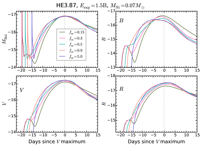
Figure 3: Light curves of bolometric, $B$-, $V$- and $R$-band magnitudes of HE3.87 SN models with an explosion energy of $1.5\times 10^{51}$ erg and a ⁵⁶Ni mass of $0.07~{}M_{\odot}$. The results with $f_{\mathrm{m}}=$0.15, 0.3, 0.5, 0.9 and 5.0 are presented using different colors as indicated by the legends in the upper-left panel.

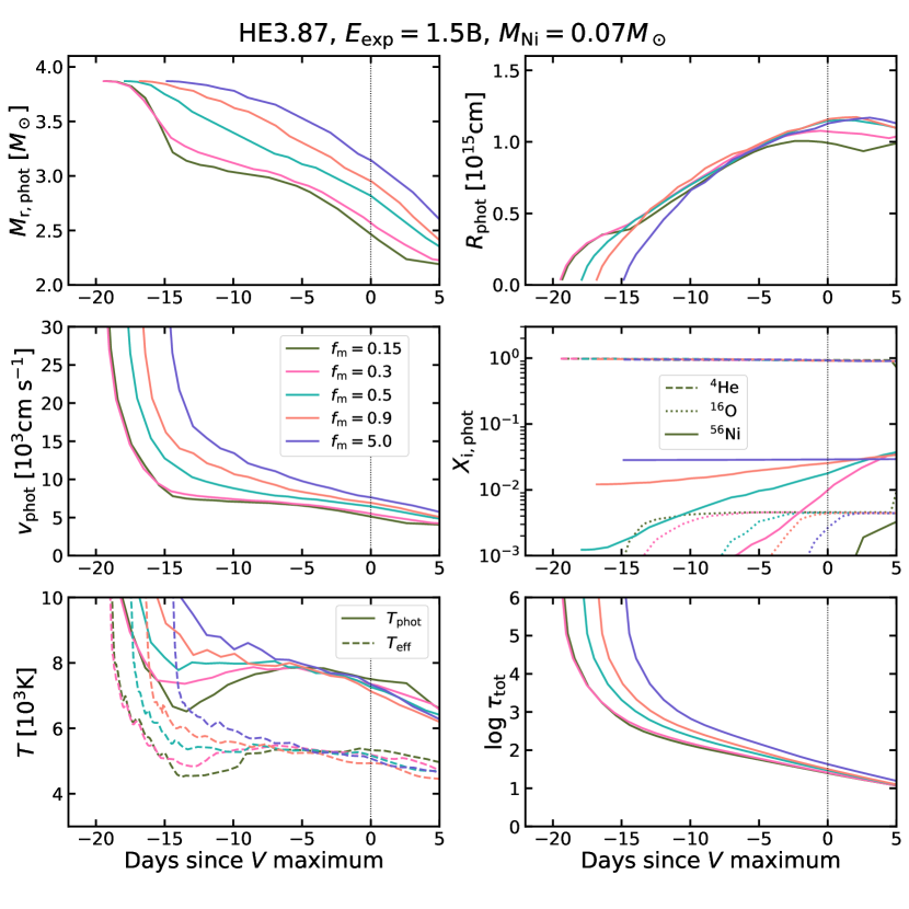
Figure 4: Evolution of the photospheric properties of HE3.87 SN models with an explosion energy of $1.5\times 10^{51}$ erg and a ⁵⁶Ni mass of $0.07~{}M_{\odot}$: mass coordinate (top-left), radius (top-right), velocity (middle-left), chemical composition (middle-right), gas temperature (bottom-left) at the photosphere. The mass coordinate in the top-left panel includes the iron core mass in the progenitor (hence the neutron star remnant mass after SN explosion). The photosphere is defined as the position where the optical depth is 2/3 calculated using the Rosseland-mean opacity. In the bottom-left panel, the effective temperatures defined by the Stefan-Boltzmann law are also given by the dotted lines for comparison. The bottom-right panel gives the total optical depth of the ejecta calculated using the Rosseland-mean opacity. The results with $f_{\mathrm{m}}=$0.15, 0.3, 0.5, 0.9 and 5.0 are presented using different colors as indicated by the legends in the middle-left panel.

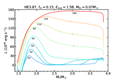
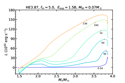
Figure 5: Evolution of the luminosity profile in the models HE3.87_fm0.15_E1.5 (upper panel) and HE3.87_fm5.0_E1.5 (lower panel). The label in each line denotes days since explosion. The vertical red line in each profile gives the position of the photosphere defined with the Rosseland mean opacity.

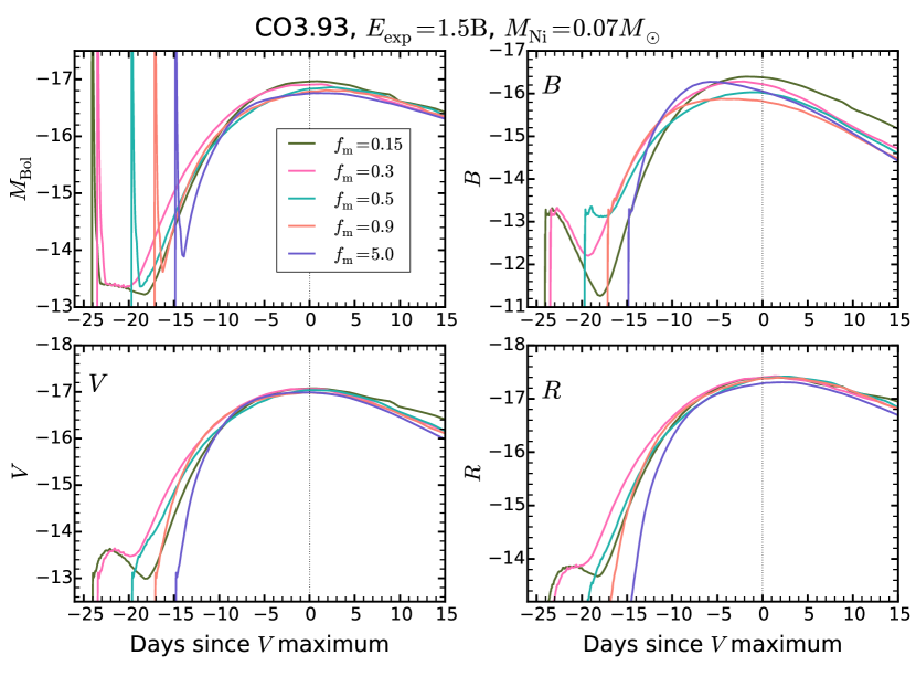
Figure 6: Same as in Figure 3 but for CO3.93 SN models.

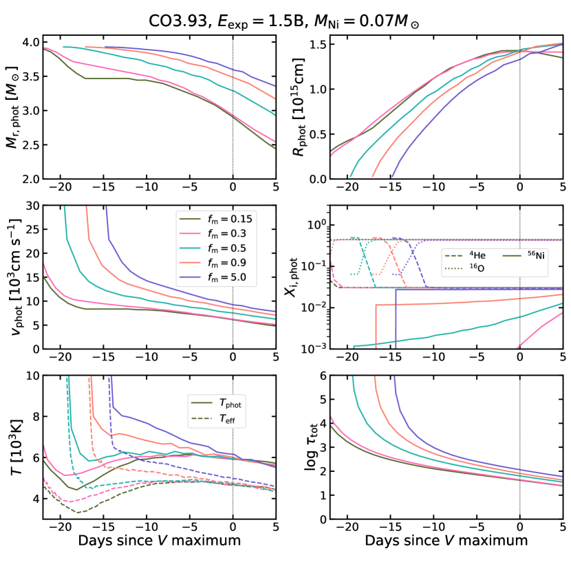
Figure 7: Same as in Figure 4 but for CO3.93 SN models.

We use the STELLA code for calculating our SN models. STELLA is a one-dimensional Lagrangian multi-group (i.e., energy dependent) radiation hydrodynamics code (Blinnikov et al., 1998, 2000, 2006) that implicitly solves the time-dependent radiation transfer equation coupled with hydrodynamics. The gamma-ray transfer is solved in a one-group approximation following Ambwani & Sutherland (1988). Positron kinetic energy is absorbed locally (see also Blinnikov et al. 1998). The maximum number of wave length bins in the code may be up to 1000, but has been fixed to 100 in our simulations, which covers from $5\times 10^{4}$Å– $10^{-3}$Å in principle. In most cases, the shortest wavelength considered in the calculations is about $0.1$Å. This is suitable to properly describe non-equilibrium continuum radiation. The ionization is obtained from a solution to the Saha equation (i.e., it assumes local thermodynamic equilibrium; LTE).

Our input models are mapped into the STELLA code using a grid of 200 – 300 mass zones. The explosion is applied by a thermal bomb at the mass cut with an explosion energy of 1.0, 1.5 and 1.8$\times 10^{51}~{}\mathrm{erg}$.

We summarize the properties of the bolometric luminosity of our SN models with $M_{\mathrm{Ni}}=0.07M_{\odot}$ in Table 2 and those of $U,B,V,R$-band magnitudes in Table 3. The input model, the mixing parameter (i.e., $f_{\mathrm{m}}$) and the explosion energy are indicated in the SN model names of the tables. For example, HE3.87_fm0.15_E1.5 means that the input model is HE3.87 and that the adopted mixing parameter and explosion energy are $f_{\mathrm{m}}=0.15$ and $E_{\mathrm{exp}}=1.5$ B, respectively. For a given explosion energy $E_{\mathrm{exp}}$, the resultant kinetic energy of the SN ($E_{\mathrm{K}}$) is lower by about $3\times 10^{50}~{}\mathrm{erg}$ for HE3.87 and $4\times 10^{50}~{}\mathrm{erg}$ for CO3.93 and CO2.12 (Table 2), which correspond to the binding energy above the mass cut in the progenitor models.

In the next two sections, we focus our discussion on the SN models with HE3.87 and CO3.93. The behavior of the SN models with CO2.12 according to different degrees of ⁵⁶Ni mixing is qualitatively similar to that of CO3.93 and we present the results with CO2.12 only for the comparison with observations, which is discussed in Section 5 below.

3 Light curves

From Table 2, we confirm the following well-known facts about SN Ib/Ic. 1) The rise time from the shock breakout to the bolometric peak ($t_{\mathrm{max}}$) and the light curve width (i.e., $\delta t_{\mathrm{Bol,+1/2}}-\delta t_{\mathrm{Bol,t-1/2}}$) become systematically smaller for a higher explosion energy for a given $f_{\mathrm{m}}$. 2) The bolometric luminosity at its peak ($L_{\mathrm{Bol,max}}$) increases with a higher explosion energy for a given $f_{\mathrm{m}}$.

Figures 3 and 4 present the light curves and the evolution of photospheric properties of HE3.87 SN models with $E_{\mathrm{exp}}=1.5\times 10^{51}~{}\mathrm{erg}$. The photosphere of a a SN Ib/Ic is not well defined (see Section 7 of Dessart et al. 2015) and in Figure 4 we present properties at the optical depth of 2/3 that is defined with the Rosseland mean opacity. In Figure 3, the shock breakout corresponds to the initial spike in the bolometric light curves. The subsequent evolution is affected by the ⁵⁶Ni distribution.

With a relatively weak mixing of ⁵⁶Ni (i.e, $f_{\mathrm{m}}=0.15$ and 0.3), a post-breakout plateau that lasts for several days is observed. This short phase is commonly observed in SN Ib/Ic models with weak or no ⁵⁶Ni mixing (Ensman & Woosley, 1988; Shigeyama et al., 1990; Dessart et al., 2011) and is powered by the release of shock deposited energy (from both radiation and internal gas energy, i.e., ionization energy from helium, carbon and oxygen) as the temperature decreases continuously. Readers are referred to Dessart et al. (2011) for a detailed discussion on this post-breakout plateau. The plateau phase comes to an end when the photosphere reaches down to the region heated by ⁵⁶Ni at about 6 d (the upper panel of Figure 5) and thereafter the bolometric luminosity starts to increase towards the main peak.

In the optical bands, the light curves with a weak ⁵⁶Ni mixing ($f_{\mathrm{m}}=0.15$ and 0.3) have double peaks (Figure 3). The first peak, which is associated with the early post-breakout evolution, is fainter than the main peak by about 1.6–2.4 mag, depending on the band. Note that this magnitude difference between the first and main peaks (in the optical) would become larger for a higher ⁵⁶Ni mass (which leads to a brighter main peak; e.g., Ensman & Woosley, 1988), or for a smaller radius of the progenitor envelope (which leads to a fainter first peak; e.g., Ensman & Woosley, 1988; Dessart et al., 2011, 2018).

For a stronger ⁵⁶Ni mixing ($f_{\mathrm{m}}\geq 0.5$), the post-breakout plateau practically disappears (see also Dessart et al., 2012). As shown in Figure 4, the mass fraction of ⁵⁶Ni at the photosphere immediately after the shock breakout is already greater than $10^{-3}$ for $f_{\mathrm{m}}\geq 0.5$ and ⁵⁶Ni heating plays the dominant role in the luminosity evolution (see the lower panel of Figure 5; Dessart et al. 2012, 2015). The time span from the shock breakout to the luminosity peak ($t_{\mathrm{Bol,max}}$ in Table 2) becomes shorter with a stronger ⁵⁶Ni mixing, while the light curve width defined by the full width at half maximum (i.e., FWHM $:=t_{\mathrm{Bol,+1/2}}-t_{\mathrm{Bol,-1/2}}$) tends to increase instead.

Figure 4 shows that the photosphere (defined here with the Rosseland mean opacity) is systematically located further out (in radius, velocity, or Lagrangian mass) for a larger $f_{\mathrm{m}}$. This is mainly because of the change in ionization caused by the extra heating in the outermost layers of the ejecta for a higher ⁵⁶Ni abundance.

The helium-deficient SN models with CO3.93 presented in Figure 6 have qualitatively similar properties to those of HE3.87. With $f_{\mathrm{m}}=0.15$ and 0.3, the post-breakout plateau is developed as in the case of HE3.87. Double peak features are also seen in the optical. The initial radius of CO3.93 ($R=0.77~{}R_{\odot}$) is much smaller than that of HE3.87 ($R=6.73~{}R_{\odot}$) and the first peaks in the optical are fainter by a factor of a few than those of HE3.87. The photosphere in CO3.93 models is systematiclly located further outward than in HE3.87 models (Figures 4 and 7). The FWHM of the bolometric light curve for a given set of $f_{\mathrm{m}}$ and $E_{\mathrm{exp}}$ is also larger in CO3.93 models (Table 2), although the CO3.93 and HE3.87 models have similar kinetic energy and ejecta mass.

4 Color evolution

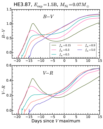
Figure 8: Evolution of $B-V$ (upper panel) and $V-R$ (lower panel) colors of HE3.87 SN models with an explosion energy of $1.5\times 10^{51}$ erg and a ⁵⁶Ni mass of $0.07~{}M_{\odot}$ since 0.05 d after the shock breakout. The results with $f_{\mathrm{m}}=$ 0.15, 0.3, 0.5, 0.9 and 5.0 are given by different colors as indicated by the legeds in the upper panel.

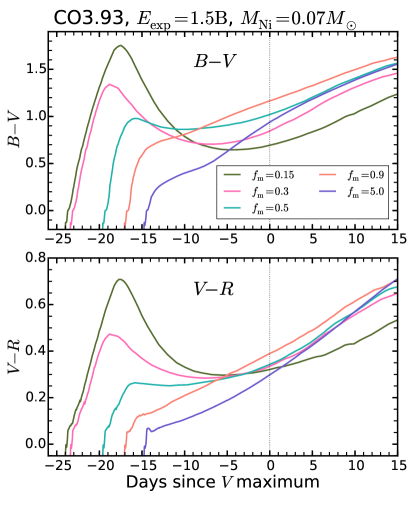
Figure 9: Same as in Figure 8 but for CO3.93 SN models.

We present the $B-V$ and $V-R$ color evolution of our HE3.87 and CO3.93 SN models with $E_{\mathrm{exp}}=1.5\times 10^{51}~{}\mathrm{erg}$ and $M_{\mathrm{Ni}}=0.07~{}M_{\odot}$ in Figures 8 and 9. Here the color evolution is shown only from 0.05 d after the shock breakout because the shock breakout features, which are practically unobservable in the optical, make the figure somewhat difficult to read clearly. The initial evolution is characterized by the rapid increase of $B-V$ and $V-R$ (i.e., the SN reddens) for all the considered $f_{\mathrm{m}}$ values. This represents the initial cooling phase due to rapid expansion with no heating source.

This initial rapid reddening phase is followed by a slope change and the subsequent evolution is affected by the ⁵⁶Ni distribution. For a weak ⁵⁶Ni mixing ($f_{\mathrm{m}}=0.15$ and 0.3), the color turns blue-ward at $t\simeq 14$ d and $18$ d before the $V$-band maximum for HE3.87 and CO3.93, respectively, because of the delayed effect of ⁵⁶Ni heating. This sign change of the slope in the color curves marks the end point of the post-breakout plateau phase and the beginning of the re-brightening shown in Figures 3 and 6. This color change in weak mixing models is also implied by the temperature evolution in Figures 4 and 7, where the photospheric temperature rapidly decreases initially and starts to increase again. The color curves reach a local minimum several days before the $V$-band maximum and the models continue to redden thereafter until the nebular phase. Observations show that the color becomes blue again $\sim 10$ d after the optical maximum as the SN enters the nebular phase  (e.g., Stritzinger et al., 2018). This phase cannot be properly described by the STELLA code because the LTE approximation for the gas breaks down (cf. Dessart et al., 2015, 2016).

For a very strong mixing of ⁵⁶Ni ($f_{\mathrm{m}}=0.9$ and 5.0), the dominant role of ⁵⁶Ni heating makes the initial reddening due to rapid expansion much weaker and the sign of the color curve slope does not change: the color continues to redden monotonically. For $f_{\mathrm{m}}=0.5$, which is the intermediate case between weak/extreme mixing, the magnitude differences after the initial reddening remain nearly constant until a few days before the $V$-band maximum and increase thereafter.

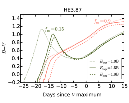
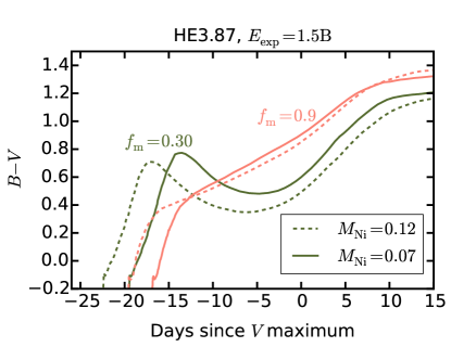
Figure 10: Upper panel: the $B-V$ color evolution of HE3.87 SN models with a ⁵⁶Ni mass of 0.07 $M_{\odot}$ and with $f_{\mathrm{m}}=0.15$ (green) and 0.90 (orange) for three different explosion energies: $E_{\mathrm{exp}}=$ 1.0 (dotted), 1.5 (solid) and 1.8 (dashed)$\times 10^{51}$ erg. Lower panel: the $B-V$ color evolution of HE3.87 SN models with an explosion energy of $1.5\times 10^{51}$ erg and with $f_{\mathrm{m}}=0.3$ (green) and 0.9 (orange) for two different ⁵⁶Ni masses: $M_{\mathrm{Ni}}=0.07$ (solid line) and $M_{\mathrm{Ni}}=0.12$ (dashed line).

In Figure 10, we compare the $B-V$ evolution of HE3.87 models for different explosion energies. A lower explosion energy leads to a longer rise time to the optical maximum and to a slightly redder color at the first peak of $B-V$, which marks the end of the initial rapid cooling phase. The color at the $V$-band maximum is not significantly affected by the explosion energy either. The figure shows that a larger amount of ⁵⁶Ni may make the SN color systematically bluer, which results from more significant ⁵⁶Ni heating, but the overall behavior of the color evolution is not affected by the total amount of ⁵⁶Ni.

We conclude that the slope change of the color curve is mainly determined by the ⁵⁶Ni distribution. This means that the color evolution before the optical maximum would provide a strong observational constraint on ⁵⁶Ni mixing in SN Ib/Ic as discussed below.

5 Comparison with observations

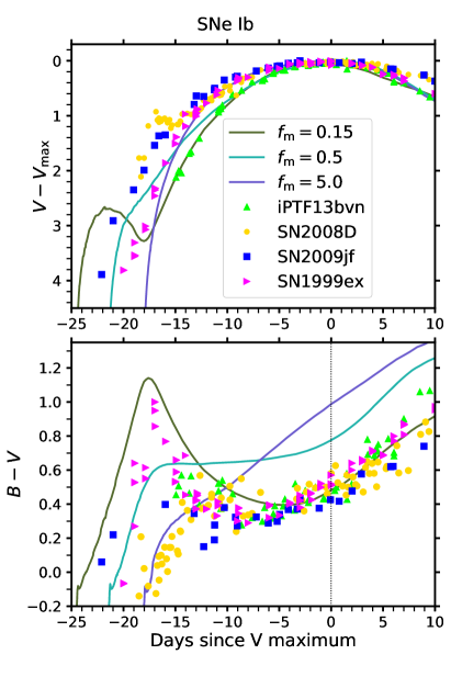
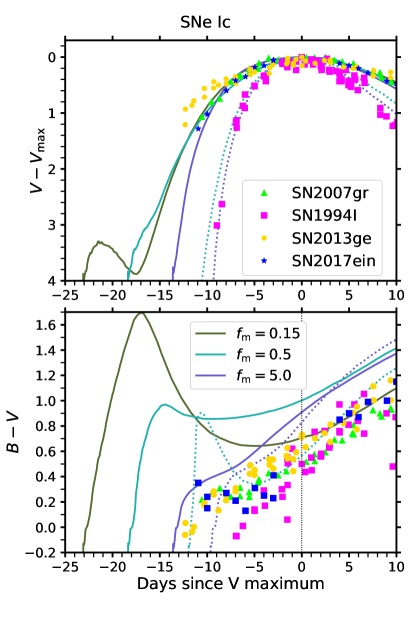
Figure 11: Upper left panel: $V$-band light curves with $V_{\mathrm{max}}$ of iPTF13bvn, SN2008D, SN2009jf, and SN 1999ex compared with HE3.87 SN models with $E_{\mathrm{exp}}=1.0\times 10^{51}$ erg and $M_{\mathrm{Ni}}=0.07M_{\odot}$. Upper right panel: SN 2007gr, SN 2013ge and SN 2017ein compared with CO3.93 SN models with $E_{\mathrm{exp}}=1.8\times 10^{51}$ erg and $M_{\mathrm{Ni}}=0.07M_{\odot}$ (solid line), and SN 1994I compared with CO2.16 models with $E_{\mathrm{exp}}=1.0\times 10^{51}$ erg and $M_{\mathrm{Ni}}=0.07M_{\odot}$ (dotted line). Lower panel: the corresponding $B-V$ color curves. The SN data are taken from the Open Supernova Catalog (https://sne.space) except SN 2007gr and SN 2017ein of which the data are from Chen et al. (2014) and Van Dyk et al. (2018), respectively. Reddening correction ($E(B-V)$) is applied for each SN as the following. iPTF13bvn: 0.12 (Fremling et al., 2016), SN2008D: 0.6 (Soderberg et al., 2008; Modjaz et al., 2009), SN2009jf: 0.16 (Valenti et al., 2011), SN 1999ex: 0.28 (Stritzinger et al., 2002), SN 2007gr: 0.085 (Chen et al., 2014), SN 1994I: 0.45 (Richmond et al., 1996), SN 2013ge: 0.067 (Drout et al., 2016), SN 2017ein: 0.34 (Van Dyk et al., 2018).

We have shown that the ⁵⁶Ni distribution in SN Ib/Ic ejecta impacts their optical color evolution during the photospheric phase. Here we confront our models with several observed SNe Ib/Ic. We do not intend to quantitatively infer physical parameters like the ejecta kinetic energy and mass, the ⁵⁶Ni mass, or the progenitor radius of each SN. Instead we focus our discussion on the color evolution in a qualitative way.

5.1 Type Ib supernovae

On the left side of Figure 11, we present the $V$-band light curves and $B-V$ color curves of 4 different SNe Ib (i.e., SN 1999ex, SN 2008D, SN 2009jf, and iPTF13bvn), compared with our HE3.87 SN models with $E_{\mathrm{exp}}=1.0$ B and $M_{\mathrm{Ni}}=0.07M_{\odot}$. These SNe Ib are very good test cases of our model predictions because they were observed from about 20 to 15 days before the $V$-band maximum.

5.1.1 SN 1999ex

The most remarkable case is SN 1999ex. As shown in the figure, the initial rapid reddening phase is unambiguously observed for a period of $t\simeq 20\cdots 17$ d before the $V$-band maximum. Then the $B-V$ color reddens until about $-$10 d before becoming blue again. Here, this behavior is matched by our weak mixing model (e.g., $f_{\mathrm{m}}=0.15$), implying that the ⁵⁶Ni distribution in the SN 1999ex ejecta is highly concentrated in the center. The double peak feature predicted in weak mixing models (Figure 3) is not found in the $V$-band light curve. However, Stritzinger et al. (2002) reports a strong signature of the post-breakout plateau in the $U-$band for this SN. It is likely that the first peak in $V$-band was missed in the SN survey because it was too faint (i.e., fainter by $>4$ mag than at the optical maximum as implied by Figure 11). As discussed in Section 3, the magnitude difference between the first and main peaks in the optical can be much larger than what is predicted by the HE3.87 SN models for a higher ⁵⁶Ni mass and/or for a more compact progenitor (e.g., Dessart et al., 2018). A more detailed study should explain the lack of an optical post-breakout plateau in a quantitative way.

Hamuy et al. (2002) classify SN 1999ex as Type Ib/c instead of Type Ib, arguing that it is an intermediate case between Ib and Ic. This is because helium lines in the optical are relatively weak compared to those of ordinary SNe Ib. The weak ⁵⁶Ni mixing evidenced by the color evolution of SN 1999ex implies that the weakness of He I lines is not necessarily due to a relatively small amount of helium. Note also that He I lines of this SN gradually become stronger as the light curve approaches its main peak as in the case of ordinary SNe Ib (Hamuy et al., 2002). This is consistent with the case of weak ⁵⁶Ni mixing in a helium-rich ejecta where thermal processes form weak He I lines initially and in later stages non-thermal processes due to radioactive decay of ⁵⁶Ni gradually become more important to make stronger He I lines (Dessart et al., 2012).

We conclude that the progenitor of SN 1999ex might have retained a fairly large amount of helium and that the relative weakness of He I lines are not necessarily due to a small content of helium.

5.1.2 iPTF13bvn

The color evolution in Figure 11 indicates that the initial rapid reddening phase is missing for iPTF13bvn. However, we observe that the color reddens from 18 d until about $13$ d before the $V$-band maximum and becomes bluer thereafter until $7$ d before the $V$-band maximum. This provides evidence for a relatively weak ⁵⁶Ni mixing. The difference in the strength of He I lines between iPTF13bvn and SN 1999ex would have resulted from somewhat different degrees of ⁵⁶Ni mixing (cf. Dessart et al., 2012). For example, both HE3.87 SN models with $f_{\mathrm{m}}=0.15$ and $f_{\mathrm{m}}=0.3$ have a similar qualitative slope change in the color evolution (Figure 8), but the influence of ⁵⁶Ni radioactive decay at the photosphere for the formation of He I lines would become more important with $f_{\mathrm{m}}=0.3$ as implied by the evolution of the chemical composition at the photosphere presented in Figure 4.

5.1.3 SN 2009jf

Early time data is available for SN 2009jf (i.e., $V-V_{\mathrm{max}}\simeq 4$ mag; Figure 11). The initial rise in the light curve from $V-V_{\mathrm{max}}\simeq 4$ mag to $V-V_{\mathrm{max}}\simeq 3$ mag is very rapid but a small decrease in the slope is observed from $V-V_{\mathrm{max}}\simeq 3$ to $V-V_{\mathrm{max}}\simeq 2.4$ mag. This behavior is qualitatively similar to the HE3.87 SN model prediction with $f_{\mathrm{m}}=0.5$. The color evolution is also qualitatively consistent with the prediction with $f_{\mathrm{m}}=0.5$, although the model prediction is much redder than the observation. Unfortunately, however, the $B-V$ data is missing for $t\simeq=19\cdots 17$ d before the $V$-band maximum, and we do not know how strong the initial reddening was. This makes it difficult to precisely determine which model is most consistent with the color evolution of this SN.

5.1.4 SN 2008D

SN 2008D is a SN Ib having very luminous post-breakout emission (Soderberg et al., 2008; Malesani et al., 2009; Modjaz et al., 2009). Bersten et al. (2013) invoked jet-induced ⁵⁶Ni mixing into high-velocity outermost layers of the ejecta to explain the early time evolution of this SN. More recently, Dessart et al. (2018) argued that the featureless spectra having weak He I lines during early times can be better explained by a helium-giant progenitor having an extended and tenuous envelope (i.e., $R\sim 200R_{\odot}$). The post-breakout plateau phase is rather short (i.e., about 3 days) and is followed by an increase in luminosity towards the main peak.

In the lower panel of Figure 11 we see that SN 2008D does not become as red as SN 1999ex at the end of the initial reddening phase (i.e., $B-V=0.5-0.6$ mag at $t\simeq-13$ d for SN 2008D compared to $B-V\simeq 0.1$ mag at $t\simeq-17$ d for SN 1999ex). In the context of our study on ⁵⁶Ni mixing, this would imply a stronger mixing in SN 2008D than in SN 1999ex, although not as extreme as assumed by Bersten et al. (2013). This property of relatively strong ejecta mixing may be compatible with the giant progenitor model proposed by Dessart et al. (2018), which is crucial to explain the large early-time brightness. Indeed, in the helium giant scenario, chemical mixing induced by the Rayleigh-Taylor instability would be more efficient (Shigeyama et al., 1990; Hachisu et al., 1991). Subsequently, the color behavior is quite similar to the other events and very strong mixing (i.e., $f_{\mathrm{m}}=0.9-5.0$) is ruled out.

5.2 Type Ic supernovae

The properties of ordinary SNe Ic, as we understand them today, are similar to those of SNe Ib in terms of kinetic energy, ejecta mass, and ⁵⁶Ni mass in general. The observed sample is heterogeneous, with a greater diversity for SNe Ic relative to SNe Ib. For example, SN 1994I, which is the prototype of SNe Ic, has an unusually short rise time. Furthermore, all SNe associated with long gamma-ray bursts (GRB) and all hydrogen-deficient hyper-energetic/superluminous SNe have been found to belong to Type Ic (Woosley & Bloom, 2006; Gal-Yam, 2012; Branch & Wheeler, 2017). So far, there is no SN Ib associated with a long GRB or hyper-energetic/superluminous SN, with the possible exceptions of SN 2016coi, which exhibits unusually broad He I lines (Yamanaka et al., 2017), and of SN 2005bf, whose high luminosity may be powered by a magnetar (e.g., Maeda et al., 2007). The origin of the SN Ic diversity is currently poorly known. Rapid core rotation in the SN progenitor may be a necessary condition for making a central engine (either collapsar or magnetar) susceptible to power a hyper-energetic/superluminous SN (Woosley, 1993; Wheeler et al., 2000). Given that our 1-D STELLA models cannot be directly compared to these peculiar SNe Ic, whose ejecta are probably highly asymmetric  (e.g., Maeda et al., 2003; Dessart et al., 2017), our discussion is limited to SNe Ic that appear to be ordinary in terms of kinetic energy ($E_{\mathrm{K}}=(1-2)\times 10^{51}$ erg) and ⁵⁶Ni mass ($M_{\mathrm{Ni}}\approx 0.1M_{\odot}$).

On the right side of Figure 11 our CO3.93 SN models with $E_{\mathrm{exp}}=1.8$ B and $M_{\mathrm{Ni}}=0.07M_{\odot}$ are compared with SN 1994I, SN 2007gr, SN 2013ge and SN 2017ein. The early-time features of these SNe are relatively well studied compared to those of other SNe Ic. The first data for SN 1994I is very deep ($V-V_{\mathrm{max}}\simeq 3.0$) but for the other three SNe Ic, we have only $V-V_{\mathrm{max}}\approx 1.0$ at the first data point, which is much smaller than in the case of SNe Ib (i.e., $V-V_{\mathrm{max}}\gtrsim 2.0$ at the first data point). Therefore, our argument presented below for these three SNe Ic is weaker than in the case of SNe Ib.

There is no clear evidence for He I lines in the optical spectra of SN 1994I, SN 2007gr and SN 2017ein, which have been classified as Type Ic. Drout et al. (2016) report weak He I lines in the early optical spectra of SN 2013ge and classify this SN as SN Ib/c. However, unlike SN 1999ex, these He I signatures soon disappear and SN 2013ge would have been classified as SN Ic without early-time spectra. This suggests that signatures of helium could have been observed in many other SNe Ic if data at earlier times had been available. The color evolution of SN 2013ge, which shows a monotonic increase in $B-V$, is qualitatively different from the SNe Ib discussed above but similar to SN 1994I.

The ejecta masses of SN 2007gr, SN2013ge and SN 2017ein are inferred to be about $2-3~{}M_{\odot}$ (Valenti et al., 2008; Mazzali et al., 2010; Drout et al., 2016; Van Dyk et al., 2018), which is comparable to that of the CO3.93 model. The caveat is that these estimates based on the light curves are subject to uncertainties (e.g., Dessart et al., 2016). Non-detection with a very deep limit is reported 5 and 7 d before the discovery of SN 2007gr and SN 2013ge, respectively (Valenti et al., 2008; Drout et al., 2016). SN 1994I has a very low ejecta mass (i.e., $M_{\mathrm{ej}}\approx 0.6-1.0M_{\odot}$; e.g., Nomoto et al. 1994; Iwamoto et al. 1994; Sauer et al. 2006) that leads to a much narrower light curve than those of SN 2007gr and SN 2013ge. The first detection of SN 1994I is likely to be within a few days from explosion (Richmond et al., 1996).

As a caveat, note that the observed $B-V$ color of our SN Ic sample is systematically bluer than the model predictions. This difference might be attributed to different ⁵⁶Ni/ejecta masses, uncertainties in the reddening correction, non-LTE effects that are not included in our STELLA models, or our mixing procedure (which affects only the ⁵⁶Ni distribution). Observations indicate significant asphericity in ordinary SNe Ib/Ic (e.g., Maund et al., 2007; Tanaka et al., 2008, 2012; Reilly et al., 2016; Tanaka et al., 2017) and multi-dimensional effects might also play an important role in the color evolution.

5.2.1 SN 1994I and SN 2013ge

As shown in Figure 11 (the bottom right panel), the $B-V$ value of SN 1994I and SN 2013ge monotonically increases from the first detection. Given that the time span between the non-detection and the discovery of these SNe is fairly short ($<1-2$ d for SN1994I and $<5$ d for SN 2013ge), it is unlikely that the signature of delayed ⁵⁶Ni heating (i.e., decrease of $B-V$ after the initial reddening phase) could have been present before the discovery. Therefore, the color evolution implies that ⁵⁶Ni is almost fully mixed in the ejecta of these SNe. This contrasts with the case of SNe Ib, for which the color behavior points to a relatively weak ⁵⁶Ni mixing.

As shown by Hachinger et al. (2012) and Dessart et al. (2012), not much helium could be hidden in SNe Ic if ⁵⁶Ni were strongly mixed in the ejecta. Therefore, our analysis leads to the conclusion that the progenitors of SN 1994I and SN 2013ge did not have a helium-rich envelope, being an almost naked carbon-oxygen core.

5.2.2 SN 2007gr and SN 2017ein

For SN 2007gr, the $B-V$ color curve is somewhat flat for $t=-10\cdots-5$ d since the $V$-band maximum, and it seems to be compatible with the case of $f=0.5$. Given the lack of earlier data for this SN, however, we cannot well constrain the degree of ⁵⁶Ni mixing based on the color evolution.

SN 2017ein has a weak signature of the effect of delayed ⁵⁶Ni heating on the $B-V$ color curve (i.e., the slight decrease of $B-V$ during $t=-12\cdots-10$ d since the $V$-band maximum). This indicates that ⁵⁶Ni mixing in this SN was weaker than in SN 1994I and SN 2013ge. Although the lack of He I lines around the $V$-band maximum might be due to weak ⁵⁶Ni mixing, the constraint set on He is weak given the lack of spectra within $\sim$ 5 d of explosion. At such times, He I lines may be produced even without non-thermal effects if the the progenitor had a massive helium-rich envelope with a very high helium mass fraction (i.e., $X_{\mathrm{He}}\gtrsim 0.9$; Dessart et al. 2011).

6 Implications for SN Ib/Ic progenitors and nickel mixing

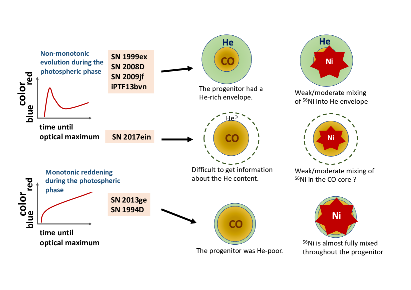
Figure 12: Schematic summary of our discussion in Section 5.

.

We schematically summarize our discussion of the previous section in Figure 12. We tentatively conclude that the color evolution of SNe Ib differs from that of SNe Ic because of different ⁵⁶Ni distributions in the ejecta. For SNe Ib, strong mixing of ⁵⁶Ni into the helium-rich envelope is ruled out and only relatively weak/moderate mixing can be compatible with observations, while very weak mixing is also ruled out as otherwise no He I lines would form at the optical maximum. For some SNe Ic (i.e., SN 1994I and SN 2013ge), ⁵⁶Ni seems to be strongly mixed throughout the SN ejecta, implying that the progenitors of these SNe Ic are intrinsically helium poor as otherwise helium could not be hidden in the spectra.

From this finding, we suggest the following propositions regarding SN Ib/Ic progenitors and ⁵⁶Ni mixing in SNe, which need to be tested by future studies:

1. Progenitors of SNe Ib and SNe Ic do not form a continuous sequence in terms of helium content in general. They differ for most cases meaning that SNe Ib progenitors have a helium-rich envelope with a high mass fraction of helium ($\gtrsim 0.9$) and SNe Ic progenitors are almost naked CO cores that only have a small amount of helium left in the outermost layers with a low mass fraction of helium.

2. Mixing of ⁵⁶Ni into the CO core during the explosion is very efficient irrespective of SN type. Hence, type Ic SNe, whose progenitors are naked CO cores, exhibit a monotonic (optical) color evolution until the nebular phase, which is a signature of strong ⁵⁶Ni mixing.

3. In progenitors having a helium-rich envelope, mixing of ⁵⁶Ni from the CO core into the helium envelope induced by hydrodynamic instabilities is probably weaker, depending on the progenitor structure.

The first proposition needs to be confronted to the predictions of stellar evolution theory. Type Ib/Ic SN progenitor models by Yoon et al. (2010) predict that the total helium mass in SN Ib/Ic progenitors decreases in a continuous way as a function of the initial mass. This is a consequence of the adopted mass-loss rate prescription for Wolf-Rayet (WR) stars given by Hamann et al. (1995) that depends only on the luminosity and the surface hydrogen abundance. Recently Yoon (2017) revisited the mass-loss rate prescription of Wolf-Rayet (WR) stars. He found that the helium mass distribution in SN Ib/Ic progenitors would be bimodal, i.e., either larger than about $1.0~{}M_{\odot}$ or less than about $0.2~{}M_{\odot}$ depending on the initial mass of the progenitors, if the mass-loss enhancement during the WC stage of WR stars compared to the case of WN stage were properly taken into account. Therefore, the first proposition is supported by the conclusion of Yoon (2017). This is also consistent with the recent observations that indicate systematic differences between SNe Ib and Ic in spectral properties (Liu et al., 2016; Prentice & Mazzali, 2017). For example, it is found that SNe Ic have a stronger absorption line O I $\lambda 7774$ and higher velocities of Fe II $\lambda 5169$ and O I $\lambda 7774$ than SNe Ib (Liu et al., 2016).

The second proposition seems to be well supported by various multi-dimensional simulations where efficient ⁵⁶Ni mixing into the CO core is often observed (e.g., Kifonidis et al., 2003, 2006; Hammer et al., 2010; Ono et al., 2013; Mao et al., 2015; Wongwathanarat et al., 2017; Müller et al., 2018). Recently Taddia et al. (2018) found that SNe Ic light curves are particularly well fitted by models with a significant ⁵⁶Ni mixing, which also supports the second proposition.

Mixing of ⁵⁶Ni into the helium envelope would depend on the progenitor structure as discussed by Shigeyama et al. (1990) and Hachisu et al. (1991). Using 2D numerical simulations, Hachisu et al. (1991) showed that ⁵⁶Ni mixing into the helium envelope due to the R-T instability in a SN progenitor having a helium-rich envelope can become more efficient for lower mass progenitors because of the higher density contrast between the CO core and the helium envelope. Almost complete mixing of ⁵⁶Ni into the helium envelope as in the cases of $f_{\mathrm{m}}=0.9$ and 5.0 of our models (Figure 1) is not found in their simulations. In their 3.3 $M_{\odot}$ helium star model where mixing occurs most efficiently in their calculations, ⁵⁶Ni is mixed only up to a middle point of the helium envelope, which is comparable to the cases of $f_{\mathrm{m}}=0.3-0.5$ in our calculations. Such moderate mixing is suitable for explaining the color evolution of SN 2008D and SN2009jf. For 6 $M_{\odot}$ helium star model, on the other hand, the R-T instability is shown to be very week and mixing occurs only in a limited region around the interface between the CO core and the helium envelope, which may well explain the properties of SN 1999ex. Therefore, the third proposition above is in good agreement with the result of Hachisu et al. (1991). However, Hachishu et al. did not consider the effects of neutrino-driven convection and ⁵⁶Ni fingers that play an important role for chemical mixing in SN ejecta (e.g., Kifonidis et al., 2003). It is also likely that the degree of ⁵⁶Ni mixing depends on the ratio of the ⁵⁶Ni mass to the SN ejecta mass (i.e., weaker mixing for a lower ⁵⁶Ni to ejecta mass ratio). Further systematic investigations of chemical mixing in SNe Ib/Ic with more realistic multi-dimensional simulations are needed.

7 Conclusions

We have discussed the effects of the ⁵⁶Ni distribution in SN ejecta on the early-time light curve and color evolution of SNe Ib/Ic. The results presented in Section 3 imply that the presence or absence of an early plateau phase can help constrain the degree of ⁵⁶Ni mixing. However, such an early plateau, if present, would be short-lived and much fainter than the main peak and would thus be easily missed. A complementary and more suitable approach is to use the early-time color evolution. We have shown that it can be a sensitive diagnostic of the ⁵⁶Ni distribution (Section 4). With a weak ⁵⁶Ni mixing, the early-time optical color initially reddens for about a week (radiation and expansion cooling is not compensated by ⁵⁶Ni heating in photospheric layers), subsequently evolves to the blue up to a week before maximum (delayed heating from ⁵⁶Ni), followed by a continuous reddening until the nebular phase. With a strong ⁵⁶Ni mixing, the effect of ⁵⁶Ni heating is more continuous and progressive, so that the color is initially bluer than in weakly mixed cases and the color reddens slowly and monotonically during the photospheric phase.

We have shown that the relatively weak/moderate ⁵⁶Ni mixing feature is found with SN 2008D, SN 2009jf, and iPTF13bvn which belong to Type Ib, while the feature of strong ⁵⁶Ni mixing is found with SN 1994I which belongs to Type Ic. Our result also implies the possibility that SN 2009ex that was considered as an intermediate case (i.e., Type Ib/c) between SN Ib and SN Ic by Hamuy et al. (2002) have relatively weak He I lines because of inefficient ⁵⁶Ni mixing into the helium envelope rather than because of a small helium content in the progenitor. On the other hand, SN 2013ge is also classified as Type Ib/c based on weak helium signature in the earliest spectra (Drout et al., 2016) but the signature of strong ⁵⁶Ni mixing in the color evolution of this SN and the disappearance of helium lines in later stages provide evidence that the progenitor did not have a helium-rich envelope.

We tentatively conclude that the population of SN Ib/Ic progenitors is largely bimodal in terms of helium content (Section 6). For further tests of our conclusions, we suggest future multi-dimensional numerical simulations of chemical mixing using realistic SN Ib/Ic progenitor models and more observations with detailed case studies of individual SNe Ib/Ic on the early-time evolution.

References

- Ambwani & Sutherland (1988) Ambwani, K., & Sutherland, P. 1988, ApJ, 325, 820, doi: 10.1086/166052
- Anderson & James (2009) Anderson, J. P., & James, P. A. 2009, MNRAS, 399, 559, doi: 10.1111/j.1365-2966.2009.15324.x
- Anderson et al. (2015) Anderson, J. P., James, P. A., Habergham, S. M., Galbany, L., & Kuncarayakti, H. 2015, PASA, 32, e019, doi: 10.1017/pasa.2015.19
- Bersten et al. (2013) Bersten, M. C., Tanaka, M., Tominaga, N., Benvenuto, O. G., & Nomoto, K. 2013, ApJ, 767, 143, doi: 10.1088/0004-637X/767/2/143
- Bersten et al. (2014) Bersten, M. C., Benvenuto, O. G., Folatelli, G., et al. 2014, AJ, 148, 68, doi: 10.1088/0004-6256/148/4/68
- Bianco et al. (2014) Bianco, F. B., Modjaz, M., Hicken, M., et al. 2014, ApJS, 213, 19, doi: 10.1088/0067-0049/213/2/19
- Blinnikov et al. (2000) Blinnikov, S., Lundqvist, P., Bartunov, O., Nomoto, K., & Iwamoto, K. 2000, ApJ, 532, 1132, doi: 10.1086/308588
- Blinnikov et al. (1998) Blinnikov, S. I., Eastman, R., Bartunov, O. S., Popolitov, V. A., & Woosley, S. E. 1998, ApJ, 496, 454, doi: 10.1086/305375
- Blinnikov et al. (2006) Blinnikov, S. I., Röpke, F. K., Sorokina, E. I., et al. 2006, A&A, 453, 229, doi: 10.1051/0004-6361:20054594
- Branch & Wheeler (2017) Branch, D., & Wheeler, J. C. 2017, Supernova Explosions, doi: 10.1007/978-3-662-55054-0
- Cao et al. (2013) Cao, Y., Kasliwal, M. M., Arcavi, I., et al. 2013, ApJ, 775, L7, doi: 10.1088/2041-8205/775/1/L7
- Chen et al. (2014) Chen, J., Wang, X., Ganeshalingam, M., et al. 2014, ApJ, 790, 120, doi: 10.1088/0004-637X/790/2/120
- Dessart et al. (2012) Dessart, L., Hillier, D. J., Li, C., & Woosley, S. 2012, MNRAS, 424, 2139, doi: 10.1111/j.1365-2966.2012.21374.x
- Dessart et al. (2011) Dessart, L., Hillier, D. J., Livne, E., et al. 2011, MNRAS, 414, 2985, doi: 10.1111/j.1365-2966.2011.18598.x
- Dessart et al. (2015) Dessart, L., Hillier, D. J., Woosley, S., et al. 2015, MNRAS, 453, 2189, doi: 10.1093/mnras/stv1747
- Dessart et al. (2016) —. 2016, MNRAS, 458, 1618, doi: 10.1093/mnras/stw418
- Dessart et al. (2017) Dessart, L., John Hillier, D., Yoon, S.-C., Waldman, R., & Livne, E. 2017, A&A, 603, A51, doi: 10.1051/0004-6361/201730873
- Dessart et al. (2018) Dessart, L., Yoon, S.-C., Livne, E., & Waldman, R. 2018, ArXiv e-prints. https://arxiv.org/abs/1801.02056
- Drout et al. (2011) Drout, M. R., Soderberg, A. M., Gal-Yam, A., et al. 2011, ApJ, 741, 97, doi: 10.1088/0004-637X/741/2/97
- Drout et al. (2016) Drout, M. R., Milisavljevic, D., Parrent, J., et al. 2016, ApJ, 821, 57, doi: 10.3847/0004-637X/821/1/57
- Eldridge et al. (2015) Eldridge, J. J., Fraser, M., Maund, J. R., & Smartt, S. J. 2015, MNRAS, 446, 2689, doi: 10.1093/mnras/stu2197
- Eldridge et al. (2013) Eldridge, J. J., Fraser, M., Smartt, S. J., Maund, J. R., & Crockett, R. M. 2013, MNRAS, 436, 774, doi: 10.1093/mnras/stt1612
- Eldridge et al. (2008) Eldridge, J. J., Izzard, R. G., & Tout, C. A. 2008, MNRAS, 384, 1109, doi: 10.1111/j.1365-2966.2007.12738.x
- Eldridge & Tout (2004) Eldridge, J. J., & Tout, C. A. 2004, MNRAS, 353, 87, doi: 10.1111/j.1365-2966.2004.08041.x
- Ensman & Woosley (1988) Ensman, L. M., & Woosley, S. E. 1988, ApJ, 333, 754, doi: 10.1086/166785
- Folatelli et al. (2016) Folatelli, G., Van Dyk, S. D., Kuncarayakti, H., et al. 2016, ApJ, 825, L22, doi: 10.3847/2041-8205/825/2/L22
- Fremling et al. (2016) Fremling, C., Sollerman, J., Taddia, F., et al. 2016, A&A, 593, A68, doi: 10.1051/0004-6361/201628275
- Gal-Yam (2012) Gal-Yam, A. 2012, Science, 337, 927, doi: 10.1126/science.1203601
- Georgy et al. (2012) Georgy, C., Ekström, S., Meynet, G., et al. 2012, A&A, 542, A29, doi: 10.1051/0004-6361/201118340
- Graur et al. (2017) Graur, O., Bianco, F. B., Huang, S., et al. 2017, ApJ, 837, 120, doi: 10.3847/1538-4357/aa5eb8
- Habergham et al. (2010) Habergham, S. M., Anderson, J. P., & James, P. A. 2010, ApJ, 717, 342, doi: 10.1088/0004-637X/717/1/342
- Hachinger et al. (2012) Hachinger, S., Mazzali, P. A., Taubenberger, S., et al. 2012, MNRAS, 422, 70, doi: 10.1111/j.1365-2966.2012.20464.x
- Hachisu et al. (1991) Hachisu, I., Matsuda, T., Nomoto, K., & Shigeyama, T. 1991, ApJ, 368, L27, doi: 10.1086/185940
- Hakobyan et al. (2009) Hakobyan, A. A., Mamon, G. A., Petrosian, A. R., Kunth, D., & Turatto, M. 2009, A&A, 508, 1259, doi: 10.1051/0004-6361/200912795
- Hakobyan et al. (2014) Hakobyan, A. A., Nazaryan, T. A., Adibekyan, V. Z., et al. 2014, MNRAS, 444, 2428, doi: 10.1093/mnras/stu1598
- Hamann et al. (1995) Hamann, W.-R., Koesterke, L., & Wessolowski, U. 1995, A&A, 299, 151
- Hammer et al. (2010) Hammer, N. J., Janka, H.-T., & Müller, E. 2010, ApJ, 714, 1371, doi: 10.1088/0004-637X/714/2/1371
- Hamuy et al. (2002) Hamuy, M., Maza, J., Pinto, P. A., et al. 2002, AJ, 124, 417, doi: 10.1086/340968
- Hirai (2017) Hirai, R. 2017, MNRAS, 466, 3775, doi: 10.1093/mnras/stw3321
- Iwamoto et al. (1994) Iwamoto, K., Nomoto, K., Höflich, P., et al. 1994, ApJ, 437, L115, doi: 10.1086/187696
- Kangas et al. (2017) Kangas, T., Portinari, L., Mattila, S., et al. 2017, A&A, 597, A92, doi: 10.1051/0004-6361/201628705
- Kelly & Kirshner (2012) Kelly, P. L., & Kirshner, R. P. 2012, ApJ, 759, 107, doi: 10.1088/0004-637X/759/2/107
- Kifonidis et al. (2003) Kifonidis, K., Plewa, T., Janka, H.-T., & Müller, E. 2003, A&A, 408, 621, doi: 10.1051/0004-6361:20030863
- Kifonidis et al. (2006) Kifonidis, K., Plewa, T., Scheck, L., Janka, H.-T., & Müller, E. 2006, A&A, 453, 661, doi: 10.1051/0004-6361:20054512
- Kim et al. (2015) Kim, H.-J., Yoon, S.-C., & Koo, B.-C. 2015, ApJ, 809, 131, doi: 10.1088/0004-637X/809/2/131
- Leloudas et al. (2011) Leloudas, G., Gallazzi, A., Sollerman, J., et al. 2011, A&A, 530, A95, doi: 10.1051/0004-6361/201116692
- Liu et al. (2016) Liu, Y.-Q., Modjaz, M., Bianco, F. B., & Graur, O. 2016, ApJ, 827, 90, doi: 10.3847/0004-637X/827/2/90
- Lucy (1991) Lucy, L. B. 1991, ApJ, 383, 308, doi: 10.1086/170787
- Lyman et al. (2016) Lyman, J. D., Bersier, D., James, P. A., et al. 2016, MNRAS, 457, 328, doi: 10.1093/mnras/stv2983
- Maeda et al. (2003) Maeda, K., Mazzali, P. A., Deng, J., et al. 2003, ApJ, 593, 931, doi: 10.1086/376591
- Maeda et al. (2007) Maeda, K., Tanaka, M., Nomoto, K., et al. 2007, ApJ, 666, 1069, doi: 10.1086/520054
- Malesani et al. (2009) Malesani, D., Fynbo, J. P. U., Hjorth, J., et al. 2009, ApJ, 692, L84, doi: 10.1088/0004-637X/692/2/L84
- Mao et al. (2015) Mao, J., Ono, M., Nagataki, S., et al. 2015, ApJ, 808, 164, doi: 10.1088/0004-637X/808/2/164
- Maund (2018) Maund, J. R. 2018, MNRAS, doi: 10.1093/mnras/sty093
- Maund et al. (2007) Maund, J. R., Wheeler, J. C., Patat, F., et al. 2007, MNRAS, 381, 201, doi: 10.1111/j.1365-2966.2007.12230.x
- Mazzali et al. (2010) Mazzali, P. A., Maurer, I., Valenti, S., Kotak, R., & Hunter, D. 2010, MNRAS, 408, 87, doi: 10.1111/j.1365-2966.2010.17133.x
- McClelland & Eldridge (2016) McClelland, L. A. S., & Eldridge, J. J. 2016, MNRAS, 459, 1505, doi: 10.1093/mnras/stw618
- Meynet & Maeder (2005) Meynet, G., & Maeder, A. 2005, A&A, 429, 581, doi: 10.1051/0004-6361:20047106
- Modjaz et al. (2009) Modjaz, M., Li, W., Butler, N., et al. 2009, ApJ, 702, 226, doi: 10.1088/0004-637X/702/1/226
- Müller et al. (2018) Müller, B., Gay, D. W., Heger, A., Tauris, T. M., & Sim, S. A. 2018, MNRAS, 479, 3675, doi: 10.1093/mnras/sty1683
- Nakar & Piro (2014) Nakar, E., & Piro, A. L. 2014, ApJ, 788, 193, doi: 10.1088/0004-637X/788/2/193
- Nomoto et al. (1994) Nomoto, K., Yamaoka, H., Pols, O. R., et al. 1994, Nature, 371, 227, doi: 10.1038/371227a0
- Nugis & Lamers (2000) Nugis, T., & Lamers, H. J. G. L. M. 2000, A&A, 360, 227
- Ono et al. (2013) Ono, M., Nagataki, S., Ito, H., et al. 2013, ApJ, 773, 161, doi: 10.1088/0004-637X/773/2/161
- Paxton et al. (2011) Paxton, B., Bildsten, L., Dotter, A., et al. 2011, ApJS, 192, 3, doi: 10.1088/0067-0049/192/1/3
- Paxton et al. (2013) Paxton, B., Cantiello, M., Arras, P., et al. 2013, ApJS, 208, 4, doi: 10.1088/0067-0049/208/1/4
- Paxton et al. (2015) Paxton, B., Marchant, P., Schwab, J., et al. 2015, ApJS, 220, 15, doi: 10.1088/0067-0049/220/1/15
- Paxton et al. (2018) Paxton, B., Schwab, J., Bauer, E. B., et al. 2018, ApJS, 234, 34, doi: 10.3847/1538-4365/aaa5a8
- Piro & Nakar (2013) Piro, A. L., & Nakar, E. 2013, ApJ, 769, 67, doi: 10.1088/0004-637X/769/1/67
- Podsiadlowski et al. (1992) Podsiadlowski, P., Joss, P. C., & Hsu, J. J. L. 1992, ApJ, 391, 246, doi: 10.1086/171341
- Prentice & Mazzali (2017) Prentice, S. J., & Mazzali, P. A. 2017, MNRAS, 469, 2672, doi: 10.1093/mnras/stx980
- Prentice et al. (2016) Prentice, S. J., Mazzali, P. A., Pian, E., et al. 2016, MNRAS, 458, 2973, doi: 10.1093/mnras/stw299
- Reilly et al. (2016) Reilly, E., Maund, J. R., Baade, D., et al. 2016, MNRAS, 457, 288, doi: 10.1093/mnras/stv3005
- Richmond et al. (1996) Richmond, M. W., van Dyk, S. D., Ho, W., et al. 1996, AJ, 111, 327, doi: 10.1086/117785
- Sanders et al. (2012) Sanders, N. E., Soderberg, A. M., Levesque, E. M., et al. 2012, ApJ, 758, 132, doi: 10.1088/0004-637X/758/2/132
- Sauer et al. (2006) Sauer, D. N., Mazzali, P. A., Deng, J., et al. 2006, MNRAS, 369, 1939, doi: 10.1111/j.1365-2966.2006.10438.x
- Shigeyama et al. (1990) Shigeyama, T., Nomoto, K., Tsujimoto, T., & Hashimoto, M.-A. 1990, ApJ, 361, L23, doi: 10.1086/185818
- Shivvers et al. (2017) Shivvers, I., Modjaz, M., Zheng, W., et al. 2017, PASP, 129, 054201, doi: 10.1088/1538-3873/aa54a6
- Smith et al. (2011) Smith, N., Li, W., Filippenko, A. V., & Chornock, R. 2011, MNRAS, 412, 1522, doi: 10.1111/j.1365-2966.2011.17229.x
- Soderberg et al. (2008) Soderberg, A. M., Berger, E., Page, K. L., et al. 2008, Nature, 453, 469, doi: 10.1038/nature06997
- Stritzinger et al. (2002) Stritzinger, M., Hamuy, M., Suntzeff, N. B., et al. 2002, AJ, 124, 2100, doi: 10.1086/342544
- Stritzinger et al. (2018) Stritzinger, M. D., Taddia, F., Burns, C. R., et al. 2018, A&A, 609, A135, doi: 10.1051/0004-6361/201730843
- Swartz (1991) Swartz, D. A. 1991, ApJ, 373, 604, doi: 10.1086/170079
- Taddia et al. (2015) Taddia, F., Sollerman, J., Leloudas, G., et al. 2015, A&A, 574, A60, doi: 10.1051/0004-6361/201423915
- Taddia et al. (2018) Taddia, F., Stritzinger, M. D., Bersten, M., et al. 2018, A&A, 609, A136, doi: 10.1051/0004-6361/201730844
- Tanaka et al. (2008) Tanaka, M., Kawabata, K. S., Maeda, K., Hattori, T., & Nomoto, K. 2008, ApJ, 689, 1191, doi: 10.1086/592325
- Tanaka et al. (2017) Tanaka, M., Maeda, K., Mazzali, P. A., Kawabata, K. S., & Nomoto, K. 2017, ApJ, 837, 105, doi: 10.3847/1538-4357/aa6035
- Tanaka et al. (2012) Tanaka, M., Kawabata, K. S., Hattori, T., et al. 2012, ApJ, 754, 63, doi: 10.1088/0004-637X/754/1/63
- Tauris et al. (2015) Tauris, T. M., Langer, N., & Podsiadlowski, P. 2015, MNRAS, 451, 2123, doi: 10.1093/mnras/stv990
- Tsvetkov et al. (2001) Tsvetkov, D. Y., Blinnikov, S. I., & Pavlyuk, N. N. 2001, Astronomy Letters, 27, 411, doi: 10.1134/1.1381608
- Valenti et al. (2008) Valenti, S., Elias-Rosa, N., Taubenberger, S., et al. 2008, ApJ, 673, L155, doi: 10.1086/527672
- Valenti et al. (2011) Valenti, S., Fraser, M., Benetti, S., et al. 2011, MNRAS, 416, 3138, doi: 10.1111/j.1365-2966.2011.19262.x
- van den Bergh et al. (2005) van den Bergh, S., Li, W., & Filippenko, A. V. 2005, PASP, 117, 773, doi: 10.1086/431435
- Van Dyk et al. (2018) Van Dyk, S. D., Zheng, W., Brink, T. G., et al. 2018, ApJ, 860, 90, doi: 10.3847/1538-4357/aac32c
- Wellstein & Langer (1999) Wellstein, S., & Langer, N. 1999, A&A, 350, 148
- Wheeler et al. (2000) Wheeler, J. C., Yi, I., Höflich, P., & Wang, L. 2000, ApJ, 537, 810, doi: 10.1086/309055
- Wongwathanarat et al. (2017) Wongwathanarat, A., Janka, H.-T., Müller, E., Pllumbi, E., & Wanajo, S. 2017, ApJ, 842, 13, doi: 10.3847/1538-4357/aa72de
- Woosley (1993) Woosley, S. E. 1993, ApJ, 405, 273, doi: 10.1086/172359
- Woosley & Bloom (2006) Woosley, S. E., & Bloom, J. S. 2006, ARA&A, 44, 507, doi: 10.1146/annurev.astro.43.072103.150558
- Woosley & Eastman (1997) Woosley, S. E., & Eastman, R. G. 1997, in NATO Advanced Science Institutes (ASI) Series C, Vol. 486, NATO Advanced Science Institutes (ASI) Series C, ed. P. Ruiz-Lapuente, R. Canal, & J. Isern, 821
- Woosley et al. (1995) Woosley, S. E., Langer, N., & Weaver, T. A. 1995, ApJ, 448, 315, doi: 10.1086/175963
- Xiao & Eldridge (2015) Xiao, L., & Eldridge, J. J. 2015, MNRAS, 452, 2597, doi: 10.1093/mnras/stv1425
- Yamanaka et al. (2017) Yamanaka, M., Nakaoka, T., Tanaka, M., et al. 2017, ApJ, 837, 1, doi: 10.3847/1538-4357/aa5f57
- Yoon (2015) Yoon, S.-C. 2015, PASA, 32, e015, doi: 10.1017/pasa.2015.16
- Yoon (2017) —. 2017, MNRAS, 470, 3970, doi: 10.1093/mnras/stx1496
- Yoon et al. (2017) Yoon, S.-C., Dessart, L., & Clocchiatti, A. 2017, ApJ, 840, 10, doi: 10.3847/1538-4357/aa6afe
- Yoon et al. (2012) Yoon, S.-C., Gräfener, G., Vink, J. S., Kozyreva, A., & Izzard, R. G. 2012, A&A, 544, L11, doi: 10.1051/0004-6361/201219790
- Yoon et al. (2010) Yoon, S.-C., Woosley, S. E., & Langer, N. 2010, ApJ, 725, 940, doi: 10.1088/0004-637X/725/1/940