ASVRG: Accelerated Proximal SVRG

Abstract

This paper proposes an accelerated proximal stochastic variance reduced gradient (ASVRG) method, in which we design a simple and effective momentum acceleration trick. Unlike most existing accelerated stochastic variance reduction methods such as Katyusha, ASVRG has only one additional variable and one momentum parameter. Thus, ASVRG is much simpler than those methods, and has much lower per-iteration complexity. We prove that ASVRG achieves the best known oracle complexities for both strongly convex and non-strongly convex objectives. In addition, we extend ASVRG to mini-batch and non-smooth settings. We also empirically verify our theoretical results and show that the performance of ASVRG is comparable with, and sometimes even better than that of the state-of-the-art stochastic methods.

1 Introduction

Consider the following composite convex minimization:

$$\min_{x\in\mathbb{R}^{d}}F(x):=f(x)+g(x)=\frac{1}{n}\!\sum_{i=1}^{n}\!f_{i}(x)+g(x),$$ (1)

where $f(x)\!:=\!\frac{1}{n}{\textstyle\sum}^{n}_{i=1}f_{i}(x)$ is a convex function that is a finite average of $n$ convex component functions $f_{i}(x)\!:\!\mathbb{R}^{d}\!\rightarrow\!\mathbb{R}$, and $g(x)$ is a “simple” possibly non-smooth convex function. This formulation naturally arises in many problems in machine learning, optimization and signal processing, such as regularized empirical risk minimization (ERM)) and eigenvector computation (Shamir, 2015; Garber et al., 2016). To solve Problem (1) with a large sum of $n$ component functions, computing the full gradient of $f(x)$ in first-order methods is expensive, and hence stochastic gradient descent (SGD) has been widely applied to many large-scale problems (Zhang, 2004; Krizhevsky et al., 2012). The update rule of proximal SGD is

$$x_{t}=\mathop{\arg\min}_{y\in\mathbb{R}^{d}}\,\left\{\frac{1}{2\eta_{t}}\|y-x_{t-1}\|^{2}+y^{T}\nabla\!f_{i_{t}}\!(x_{t-1})+g(y)\right\},$$ (2)

where $\eta_{t}\!\propto\!1/\sqrt{t}$ is the step size, and $i_{t}$ is chosen uniformly at random from $\{1,\ldots,n\}$. When $g(x)\!\equiv\!0$, the update rule in (2) becomes $x_{t}\!=\!x_{t-1}\!-\!\eta_{t}\nabla\!f_{i_{t}}\!(x_{t-1})$. The standard SGD estimates the gradient from just one example (or a mini-batch), and thus it enjoys a low per-iteration cost as opposed to full gradient methods. The expectation of $\nabla\!f_{i}(x_{t})$ is an unbiased estimation to $\nabla\!f(x_{t})$, i.e., $\mathbb{E}[\nabla\!f_{i}(x_{t})]\!\!=\!\!\nabla\!f(x_{t})$. However, the variance of the stochastic gradient estimator may be large, which leads to slow convergence (Johnson and Zhang, 2013). Even under the strongly convex (SC) and smooth conditions, standard SGD can only attain a sub-linear rate of convergence (Rakhlin et al., 2012; Shamir and Zhang, 2013).

Recently, the convergence rate of SGD has been improved by many variance reduced SGD methods (Roux et al., 2012; Shalev-Shwartz and Zhang, 2013; Johnson and Zhang, 2013; Defazio et al., 2014a; Mairal, 2015) and their proximal variants (Schmidt et al., 2013; Xiao and Zhang, 2014; Shalev-Shwartz and Zhang, 2016). The methods use past gradients to progressively reduce the variance of stochastic gradient estimators, so that a constant step size can be used. In particular, these variance reduced SGD methods converge linearly for SC and Lipschitz-smooth problems. SVRG (Johnson and Zhang, 2013) and its proximal variant, Prox-SVRG (Xiao and Zhang, 2014), are particularly attractive because of their low storage requirement compared with the methods in (Roux et al., 2012; Defazio et al., 2014a; Shalev-Shwartz and Zhang, 2016), which need to store all the gradients of the $n$ component functions $f_{i}(\cdot)$ (or dual variables), so that $O(nd)$ storage is required in general problems. At the beginning of each epoch of SVRG and Prox-SVRG, the full gradient $\nabla\!f(\widetilde{x})$ is computed at the past estimate $\widetilde{x}$. Then the key update rule is given by

$$\begin{split}&\quad\,\widetilde{\nabla}\!f_{i_{t}}\!(x_{t-1})=\nabla\!f_{i_{t}}\!(x_{t-1})-\nabla\!f_{i_{t}}\!(\widetilde{x})+\nabla\!f(\widetilde{x}),\\ &x_{t}=\mathop{\arg\min}_{y\in\mathbb{R}^{d}}\,\left\{\frac{1}{2\eta}\|y-x_{t-1}\|^{2}+y^{T}\widetilde{\nabla}\!f_{i_{t}}\!(x_{t-1})+g(y)\right\}.\end{split}$$ (3)

For SC problems, the oracle complexity (total number of component gradient evaluations to find $\varepsilon$-suboptimal solutions) of most variance reduced SGD methods is $\mathcal{O}\!\left((n\!+\!{L}/{\mu})\log({1}/{\varepsilon})\right)$, when each $f_{i}(x)$ is $L$-smooth and $g(x)$ is $\mu$-strongly convex. Thus, there still exists a gap between the oracle complexity and the upper bound in (Woodworth and Srebro, 2016). In theory, they also converge slower than accelerated deterministic algorithms (e.g., FISTA (Beck and Teboulle, 2009)) for non-strongly convex (non-SC) problems, namely $\mathcal{O}(1/t)$ vs. $\mathcal{O}(1/t^{2})$.

Very recently, several advanced techniques were proposed to further speed up the variance reduction SGD methods mentioned above. These techniques mainly include the Nesterov’s acceleration technique (Nitanda, 2014; Lin et al., 2015; Murata and Suzuki, 2017; Lan and Zhou, 2018), the projection-free property of the conditional gradient method (Hazan and Luo, 2016), reducing the number of gradient calculations in the early iterations (Babanezhad et al., 2015; Allen-Zhu and Yuan, 2016; Shang et al., 2017), and the momentum acceleration trick (Hien et al., 2018; Allen-Zhu, 2018; Zhou et al., 2018; Shang et al., 2018b). Lin et al. (2015) and Frostig et al. (2015) proposed two accelerated algorithms with improved oracle complexity of $\mathcal{O}((n+\sqrt{n{L}/{\mu}})\log({L}/{\mu})\log({1}/{\varepsilon}))$ for SC problems. In particular, Katyusha (Allen-Zhu, 2018) attains the optimal oracle complexities of $\mathcal{O}((n\!+\!\!\sqrt{n{L}/{\mu}})\log({1}/{\varepsilon}))$ and $\mathcal{O}(n\log({1}/{\varepsilon})\!+\!\sqrt{nL/\varepsilon})$ for SC and non-SC problems, respectively. The main update rules of Katyusha are formulated as follows:

$$\begin{split}&x_{t}=y_{t-1}+\omega_{1}(z_{t-1}-y_{t-1})+\omega_{2}(\widetilde{x}-y_{t-1}),\\ &y_{t}=\mathop{\arg\min}_{y\in\mathbb{R}^{d}}\,\left\{\frac{3L}{2}\|y-x_{t}\|^{2}+y^{T}\widetilde{\nabla}\!f_{i_{t}}\!(x_{t})+g(y)\right\},\\ &z_{t}=\mathop{\arg\min}_{z\in\mathbb{R}^{d}}\,\left\{\frac{1}{2\eta}\|z-z_{t-1}\|^{2}+z^{T}\widetilde{\nabla}\!f_{i_{t}}\!(x_{t})+g(z)\right\},\end{split}$$ (4)

where $\omega_{1},\omega_{2}\!\in\![0,1]$ are two parameters for the key momentum terms, and $\eta\!=\!1/(3\omega_{1}L)$. Note that the parameter $\omega_{2}$ is fixed to $0.5$ in (Allen-Zhu, 2018) to avoid parameter tuning.

Our Contributions. In spite of the success of momentum acceleration tricks, most of existing accelerated methods including Katyusha require at least two auxiliary variables and two corresponding momentum parameters (e.g., for the Nesterov’s momentum and Katyusha momentum in (4)), which lead to complicated algorithm design and high per-iteration complexity. We address the weaknesses of the existing methods by a simper accelerated proximal stochastic variance reduced gradient (ASVRG) method, which requires only one auxiliary variable and one momentum parameter. Thus, ASVRG leads to much simpler algorithm design and is more efficient than the accelerated methods. Impressively, ASVRG attains the same low oracle complexities as Katyusha for both SC and non-SC objectives. We summarize our main contributions as follows.

• We design a simple momentum acceleration trick to accelerate the original SVRG. Different from most accelerated algorithms such as Katyusha, which require two momentums mentioned above, our update rule has only one momentum accelerated term.

• We prove that ASVRG converges to an $\varepsilon$-minimizer with the oracle complexity of $\mathcal{O}((n\!+\!\sqrt{n{L}/{\mu}})\log({1}/{\varepsilon}))$ for SC problems, which is the same as that in (Defazio, 2016; Allen-Zhu, 2018), and matches the upper bound in (Woodworth and Srebro, 2016).

• We also prove that ASVRG achieves the optimal convergence rate of $\mathcal{O}(1/t^{2})$ and the oracle complexity of $\mathcal{O}(n\log({1}/{\varepsilon})\!+\!\sqrt{nL/\varepsilon})$ for non-SC problems, which is identical to the best known result in (Hien et al., 2018; Allen-Zhu, 2018).

• Finally, we introduce mini-batching, adaptive regularization and smooth techniques into our algorithms, and further analyze their convergence properties and summarize the oracle complexities of ASVRG for the four cases of Problem (1) in Table 2.

Table 1: Comparison of the oracle complexities of some stochastic variance reduced algorithms for the four classes of problems in Section 2. Note that $C_{1}\!\!=\!\|\widetilde{x}^{0}\!-\!x^{\star}\|$ and $C_{2}\!\!=\!F(\widetilde{x}^{0})\!-\!F(x^{\star})$.

	$L$-Smooth		$G$-Lipschitz
	​​​​$\mu$-Strongly Convex	​​​​​​​non-SC	$\mu$-Strongly Convex	​​​​​​​non-SC ​​​​
SVRG​​	​​​​$\mathcal{O}\!\left((n\!+\!{L}/{\mu})\log\!\frac{C_{2}}{\varepsilon}\right)$	​​​​​​​ unknown	​​​​ unknown	​​​​​​​ unknown​​​​
SAGA​​	​​​​$\mathcal{O}\!\left((n\!+\!{L}/{\mu})\log\!\frac{C_{2}}{\varepsilon}\right)$	​​​​​​​ $\mathcal{O}\!\left({nC_{2}}/{\varepsilon}\!+\!{LC^{2}_{1}}/{\varepsilon}\right)$	​​​​ unknown	​​​​​​​ unknown​​​​
Katyusha​​	​​$\mathcal{O}\!\left((n\!+\!\!\sqrt{n{L}/{\mu}})\log\!\frac{C_{2}}{\varepsilon}\right)$	​​​​​​​ $\mathcal{O}\!\left(n\log\!\frac{C_{2}}{\varepsilon}\!+\!C_{1}\!\sqrt{{nL}/{\varepsilon}}\right)$​​​	​​​​ $\mathcal{O}\!\left(n\log\!\frac{C_{2}}{\varepsilon}\!+\!\frac{\sqrt{n}G}{\sqrt{\mu\varepsilon}}\right)$	​​​​​​​ $\mathcal{O}\!\left(n\log\frac{C_{2}}{\varepsilon}\!+\!\frac{\sqrt{n}C_{1}G}{\varepsilon}\right)$​​​​
ASVRG​​	​​$\mathcal{O}\!\left((n\!+\!\!\sqrt{n{L}/{\mu}})\log\!\frac{C_{2}}{\varepsilon}\right)$	​​​​​​​ $\mathcal{O}\!\left(n\log\!\frac{C_{2}}{\varepsilon}\!+\!C_{1}\!\sqrt{{nL}/{\varepsilon}}\right)$​​​	​​​​ $\mathcal{O}\!\left(n\log\!\frac{C_{2}}{\varepsilon}\!+\!\frac{\sqrt{n}G}{\sqrt{\mu\varepsilon}}\right)$	​​​​​​​ $\mathcal{O}\!\left(n\log\!\frac{C_{2}}{\varepsilon}\!+\!\frac{\sqrt{n}C_{1}G}{\varepsilon}\right)$​​​​

2 Preliminaries

Throughout this paper, we use $\|\cdot\|$ to denote the standard Euclidean norm. $\nabla\!f(x)$ denotes the full gradient of $f(x)$ if it is differentiable, or $\partial\!f(x)$ the subgradient if $f(x)$ is Lipschitz continuous. We mostly focus on the case of Problem (1) when each component function $f_{i}(x)$ is $L_{i}$-smooth, and $g(x)$ is $\mu$-strongly convex.

Assumption 1

Each convex component function $f_{i}(\cdot)$ is $L_{i}$-smooth, if there exists a constant $L_{i}\!>\!0$ such that for all $x,y\!\in\!\mathbb{R}^{d}$, $\|\nabla f_{i}(x)-\nabla f_{i}(y)\|\leq L_{i}\|x-y\|$.

Assumption 2

$g(\cdot)$ is $\mu$-strongly convex ($\mu$-SC), if there exists a constant $\mu\!>\!0$ such that for any $x,y\!\in\!\mathbb{R}^{d}$ and any (sub)gradient $\xi$ (i.e., $\xi\!=\!\nabla\!g(x)$, or $\xi\!\in\!\partial g(x)$) of $g(\cdot)$ at $x$

$$g(y)\geq g(x)+\xi^{T}(y-x)+\frac{\mu}{2}\|x-y\|^{2}.$$

For a non-strongly convex function, the above inequality can always be satisfied with $\mu\!=\!0$. As summarized in (Allen-Zhu and Hazan, 2016), there are mainly four interesting cases of Problem (1):

• Case 1: Each $f_{i}(x)$ is $L_{i}$-smooth and $g(x)$ is $\mu$-SC, e.g., ridge regression, logistic regression, and elastic net regularized logistic regression.

• Case 2: Each $f_{i}(x)$ is $L_{i}$-smooth and $g(x)$ is non-SC, e.g., Lasso and $\ell_{1}$-norm regularized logistic regression.

• Case 3: Each $f_{i}(x)$ is non-smooth (but Lipschitz continuous) and $g(x)$ is $\mu$-SC, e.g., linear support vector machine (SVM).

• Case 4: Each $f_{i}(x)$ is non-smooth (but Lipschitz continuous) and $g(x)$ is non-SC, e.g., $\ell_{1}$-norm SVM.

3 Accelerated Proximal SVRG

In this section, we propose an accelerated proximal stochastic variance reduced gradient (ASVRG) method with momentum acceleration for solving both strongly convex and non-strongly convex objectives (e.g., Cases 1 and 2). Moreover, ASVRG incorporates a weighted sampling strategy as in (Xiao and Zhang, 2014; Zhao and Zhang, 2015; Shamir, 2016) to randomly pick $i_{t}$ based on a general distribution $\{p_{i},\ldots,p_{n}\}$ rather than the uniform distribution.

3.1 Iterate Averaging for Snapshot

Like SVRG, our algorithms are also divided into $S$ epochs, and each epoch consists of $m$ stochastic updates, where $m$ is usually chosen to be $\Theta(n)$ as in Johnson and Zhang (2013). Within each epoch, a full gradient $\nabla\!f(\widetilde{x}^{s-1})$ is calculated at the snapshot $\widetilde{x}^{s-1}$. Note that we choose $\widetilde{x}^{s-1}$ to be the average of the past $t$ stochastic iterates rather than the last iterate because it has been reported to work better in practice (Xiao and Zhang, 2014; Flammarion and Bach, 2015; Allen-Zhu and Yuan, 2016; Liu et al., 2017; Allen-Zhu, 2018; Shang et al., 2018b). In particular, one of the effects of the choice, i.e., $\widetilde{x}^{s}\!=\!\frac{1}{m}\!\sum^{m}_{t=1}\!x^{s}_{t}$, is to allow taking larger step sizes, e.g., $1/(3L)$ for ASVRG vs. $1/(10L)$ for SVRG.

3.2 ASVRG in Strongly Convex Case

We first consider the case of Problem (1) when each $f_{i}(\cdot)$ is $L_{i}$-smooth, and $g(\cdot)$ is $\mu$-SC. Different from existing accelerated methods such as Katyusha (Allen-Zhu, 2018), we propose a much simpler accelerated stochastic algorithm with momentum, as outlined in Algorithm 1. Compared with the initialization of $x^{s}_{0}\!=\!y^{s}_{0}\!=\!\widetilde{x}^{s-1}$ (i.e., Option I in Algorithm 1), the choices of $x^{s+1}_{0}\!=(1\!-\!\omega)\widetilde{x}^{s}+\omega y^{s}_{m_{s}}$ and $y^{s+1}_{0}\!=\!y^{s}_{m_{s}}$ (i.e., Option II) also work well in practice.

Algorithm 1 ASVRG for strongly convex objectives

0:  The number of epochs $S$, the number of iterations $m$ per epoch, and the step size $\eta$.

0:  $\widetilde{x}^{0}\!=x^{0}_{0}=y^{0}_{0}$,  $\omega$,  $m_{1}$,  $\rho\geq 1$, and the probability $P=[p_{1},\ldots,p_{n}]$.

1:  for $s=1,2,\ldots,S$ do

2:     $\widetilde{\mu}=\frac{1}{n}\!\sum^{n}_{i=1}\!\nabla\!f_{i}(\widetilde{x}^{s-1})$;

3:     Option I:  $x^{s}_{0}=y^{s}_{0}=\widetilde{x}^{s-1}$;

4:     for $t=1,2,\ldots,m_{s}$ do

5:        Pick $i_{t}$ from $\{1,\ldots,n\}$ randomly based on $P$;

6:        $\widetilde{\nabla}\!f_{i_{t}}(x^{s}_{t-1})=[\nabla\!f_{i_{t}}(x^{s}_{t-1})-\nabla\!f_{i_{t}}(\widetilde{x}^{s-1})]/(np_{i_{t}})+\widetilde{\mu}$;

7:        $y^{s}_{t}=\mathop{\arg\min}_{y}\left\{\langle\widetilde{\nabla}\!f_{i_{t}}(x^{s}_{t-1}),\,y-y^{s}_{t-1}\rangle+\frac{\omega}{2\eta}\|y-y^{s}_{t-1}\|^{2}+g(y)\right\}$;

8:        $x^{s}_{t}=\widetilde{x}^{s-1}+\omega(y^{s}_{t}-\widetilde{x}^{s-1})$;

9:     end for

10:     $\widetilde{x}^{s}\!=\frac{1}{m_{s}}\!\sum^{m_{s}}_{t=1}\!x^{s}_{t}$,  $m_{s+1}\!=\min(\lfloor\rho m_{s}\rfloor,m)$;

11:     Option II:  $x^{s+1}_{0}\!=(1\!-\!\omega)\widetilde{x}^{s}+\omega y^{s}_{m_{s}}$, and  $y^{s+1}_{0}\!=y^{s}_{m_{s}}$;

12:  end for

12:  $\widetilde{x}^{S}$.

3.2.1 Momentum Acceleration

The update rule of $y$ in our proximal stochastic gradient method is formulated as follows:

$$\begin{split}y^{s}_{t}=\mathop{\arg\min}_{y\in\mathbb{R}^{d}}\left\{\langle\widetilde{\nabla}\!f_{i_{t}}(x^{s}_{t-1}),\,y-y^{s}_{t-1}\rangle\!+\!\frac{\omega}{2\eta}\|y-y^{s}_{t-1}\|^{2}+g(y)\right\},\end{split}$$ (5)

where $\omega\!\in\![0,1]$ is the momentum parameter. Note that the gradient estimator $\widetilde{\nabla}\!f_{i_{t}}$ used in this paper is the SVRG estimator in (3). Besides, the algorithms and convergence results of this paper can be generalized to the SAGA estimator in (Defazio et al., 2014a). When $g(x)\!\equiv\!0$, the proximal update rule in (5) degenerates to $y^{s}_{t}\!=y^{s}_{t-1}\!-\!(\eta/{\omega})\widetilde{\nabla}\!f_{i_{t}}\!(x^{s}_{t-1})$.

Inspired by the Nesterov’s momentum in (Nesterov, 1983, 2004; Nitanda, 2014; Shang et al., 2018a) and Katyusha momentum in (Allen-Zhu, 2018), we design a update rule for $x$ as follows:

$$x^{s}_{t}=\widetilde{x}^{s-1}+\omega(y^{s}_{t}-\widetilde{x}^{s-1}).$$ (6)

The second term on the right-hand side of (6) is the proposed momentum similar to the Katyusha momentum in (Allen-Zhu, 2018). It is clear that there is only one momentum parameter $\omega$ in our algorithm, compared with the two parameters $\omega_{1}$ and $\omega_{2}$ in Katyusha.

The per-iteration complexity of ASVRG is dominated by the computation of $\nabla\!f_{i_{t}}\!(x^{s}_{t-1})$ and $\nabla\!f_{i_{t}}\!(\widetilde{x}^{s-1})$, and the proximal update in (5), which is as low as that of SVRG (Johnson and Zhang, 2013) and Prox-SVRG (Xiao and Zhang, 2014). In other words, ASVRG has a much lower per-iteration complexity than most of accelerated stochastic methods (Murata and Suzuki, 2017; Allen-Zhu, 2018) such as Katyusha (Allen-Zhu, 2018), which has one more proximal update for $z$ in general.

3.2.2 Momentum Parameter

Next we give a selection scheme for the stochastic momentum parameter $\omega$. With the given $\eta$, $\omega$ can be a constant, and must satisfy the inequality: $0\!<\!\omega\!\leq\!1\!-\!\frac{\widetilde{L}\eta}{1-\widetilde{L}\eta}$, where $\widetilde{L}\!=\!\max_{j}L_{j}/(np_{j})$. As shown in Theorem 4.2 below, it is desirable to have a small convergence factor $\rho$. The following proposition obtains the optimal $\omega_{\star}$, which yields the smallest $\rho$ value.

Proposition 3.1.

Given a suitable learning rate $\eta$, the optimal parameter $\omega_{\star}$ is $\omega_{\star}\!=\!m\mu\eta/2$.

In fact, we can fix $\omega$ to a constant, e.g., $0.9$, which works well in practice as in (Ruder, 2017). When $\omega\!=\!1$ and $g(x)$ is smooth, Algorithm 1 degenerates to Algorithm 3 in the supplementary material, which is almost identical to SVRG (Johnson and Zhang, 2013), and the only differences between them are the choice of $\widetilde{x}^{s}$ and the initialization of $x^{s}_{0}$.

Algorithm 2 ASVRG for non-strongly convex objectives

0:  The number of epochs $S$, the number of iterations $m$ per epoch, and the step size $\eta$.

0:  $\widetilde{x}^{0}\!=\widetilde{y}^{0}$, $\omega_{0}=1\!-\!\frac{\widetilde{L}\eta}{1-\widetilde{L}\eta}$, $m_{1}$, $\rho\geq 1$, and $P=[p_{1},\ldots,p_{n}]$.

1:  for $s=1,2,\ldots,S$ do

2:     $\widetilde{\mu}=\frac{1}{n}\!\sum^{n}_{i=1}\!\!\nabla\!f_{i}(\widetilde{x}^{s-1})$,  $x^{s}_{0}=(1\!-\!\omega_{s-1})\widetilde{x}^{s-1}+\omega_{s-1}\widetilde{y}^{s-1}$,  $y^{s}_{0}=\widetilde{y}^{s-1}$;

3:     for $t=1,2,\ldots,m_{s}$ do

4:        Pick $i_{t}$ from $\{1,\ldots,n\}$ randomly based on $P$;

5:        $\widetilde{\nabla}\!f_{i_{t}}(x^{s}_{t-1})=[\nabla\!f_{i_{t}}(x^{s}_{t-1})-\nabla\!f_{i_{t}}(\widetilde{x}^{s-1})]/(np_{i_{t}})+\widetilde{\mu}$;

6:        $y^{s}_{t}=\mathop{\arg\min}_{y}\left\{\langle\widetilde{\nabla}\!f_{i_{t}}(x^{s}_{t-1}),\,y-y^{s}_{t-1}\rangle+\frac{\omega}{2\eta}\|y-y^{s}_{t-1}\|^{2}+g(y)\right\}$;

7:        $x^{s}_{t}=\widetilde{x}^{s-1}+\omega_{s-1}(y^{s}_{t}-\widetilde{x}^{s-1})$;

8:     end for

9:     $\widetilde{x}^{s}\!=\frac{1}{m_{s}}\!\sum^{m_{s}}_{t=1}\!x^{s}_{t}$,  $\widetilde{y}^{s}\!=y^{s}_{m_{s}}$,  $\omega_{s}\!=\frac{\sqrt{\omega^{4}_{s-1}+4\omega^{2}_{s-1}}-\;\!\omega^{2}_{s-1}}{2}$,  $m_{s+1}\!=\min(\lfloor\rho m_{s}\rfloor,m)$;

10:  end for

10:  $\widetilde{x}^{S}$.

3.3 ASVRG in Non-Strongly Convex Case

We also develop an efficient algorithm for solving non-SC problems, as outlined in Algorithm 2. The main difference between Algorithms 1 and 2 is the setting of the momentum parameter. That is, the momentum parameter $\omega_{s}$ in Algorithm 2 is decreasing, while that of Algorithm 1 can be a constant. Different from Algorithm 1, $\omega_{s}$ in Algorithm 2 needs to satisfy the following inequalities:

$$\frac{1-\omega_{s}}{\omega^{2}_{s}}\leq\frac{1}{\omega^{2}_{s-\!1}}\;\,\textup{and}\;\,0\leq\omega_{s}\leq 1-\frac{\widetilde{L}\eta}{1-\widetilde{L}\eta}.$$ (7)

It is clear that the condition (7) allows the stochastic momentum parameter to decrease, but not too fast, similar to the requirement on the step-size $\eta_{t}$ in classical SGD. Unlike deterministic acceleration methods, where $\omega_{s}$ is only required to satisfy the first inequality in (7), the momentum parameter $\omega_{s}$ in Algorithm 2 must satisfy both inequalities. Inspired by the momentum acceleration techniques in (Tseng, 2010; Su et al., 2014) for deterministic optimization, the update rule for $\omega_{s}$ is defined as follows: $\omega_{0}\!=\!1\!-\!{\widetilde{L}\eta}/({1\!-\!\widetilde{L}\eta})$, and for any $s\!>\!1$, $\omega_{s}\!=\!\frac{\sqrt{\omega^{4}_{s-1}+4\omega^{2}_{s-1}}-\omega^{2}_{s-1}}{2}$.

4 Convergence Analysis

In this section, we provide the convergence analysis of ASVRG for both strongly convex and non-strongly convex objectives. We first give the following key intermediate result (the proofs to all theoretical results in this paper are given in the supplementary material).

Lemma 4.1.

Suppose Assumption 1 holds. Let $x^{\star}$ be an optimal solution of Problem (1), and $\{(x^{s}_{t},y^{s}_{t})\}$ be the sequence generated by Algorithms 1 and 2 with $\omega_{s}\leq 1\!-\!\frac{\widetilde{L}\eta}{1-\widetilde{L}\eta}$. Then for all $s\!=\!1,\ldots,S$,

$$\begin{split}\mathbb{E}\!\left[F(\widetilde{x}^{s})\!-\!F(x^{\star})\right]\leq(1\!-\!\omega_{s-1})\mathbb{E}\!\left[F(\widetilde{x}^{s-1})-F(x^{\star})\right]\!+\frac{\omega^{2}_{s-1}}{2m\eta}\mathbb{E}\!\left[\|x^{\star}\!-y^{s}_{0}\|^{2}\!-\!\|x^{\star}\!-y^{s}_{m}\|^{2}\right]\!.\end{split}$$

4.1 Analysis for Strongly Convex Objectives

For strongly convex objectives, our first main result is the following theorem, which gives the convergence rate and oracle complexity of Algorithm 1.

Theorem 4.2.

Suppose Assumptions 1 and 2 hold, and given the same notation as in Lemma 4.1, and $m$ is sufficiently large so that

$$\rho:=\,1-\omega+\frac{\omega^{2}}{m\mu\eta}<1.$$

Then Algorithm 1 with Option I has the following geometric convergence in expectation:

$$\mathbb{E}\!\left[F(\widetilde{x}^{s})-F(x^{\star})\right]\leq\,\rho^{s}\!\left[F(\widetilde{x}^{0})-F(x^{\star})\right].$$

Theorem 4.2 shows that Algorithm 1 with Option I achieves linear convergence for strongly convex problems. We can easily obtain a similar result for Algorithm 1 with Option II. The following results give the oracle complexities of Algorithm 1 with Option I or Option II, as shown in Figure 1, where $\kappa\!=\!\widetilde{L}/\mu$ is the condition number.

Corollary 4.3.

The oracle complexity of Algorithm 1 with Option I to achieve an $\varepsilon$-suboptimal solution (i.e., $\mathbb{E}\!\left[F(\widetilde{x}^{s})\right]-F(x^{\star})\leq\varepsilon$) is

$$\begin{cases}\mathcal{O}\big{(}\sqrt{{n\widetilde{L}}/{\mu}}\log{\frac{F(\tilde{x}^{0})-F(x^{\star})}{\varepsilon}}\big{)},&\;\;\;\,\text{if }\,{m\mu}/{\widetilde{L}}\!\in\![0.68623,145.72],\\ \mathcal{O}\big{(}(n+{\widetilde{L}}/{\mu})\log{\frac{F(\tilde{x}^{0})-F(x^{\star})}{\varepsilon}}\big{)},&\quad\text{otherwise}.\end{cases}$$

Corollary 4.4.

The oracle complexity of Algorithm 1 with Option II and restarts every $\mathcal{S}=2\cdot\big{(}\frac{1-\omega}{\omega}+\frac{\omega}{\eta m\mu}\big{)}$ epochs to achieve an $\varepsilon$-suboptimal solution (i.e., $\mathbb{E}\!\left[F(\widetilde{x}^{s})\right]-F(x^{\star})\leq\varepsilon$) is

$$\mathcal{O}\big{(}(n\!+\!\sqrt{{n\widetilde{L}}/{\mu}})\log{\frac{F(\tilde{x}^{0})-F(x^{\star})}{\varepsilon}}\big{)}.$$

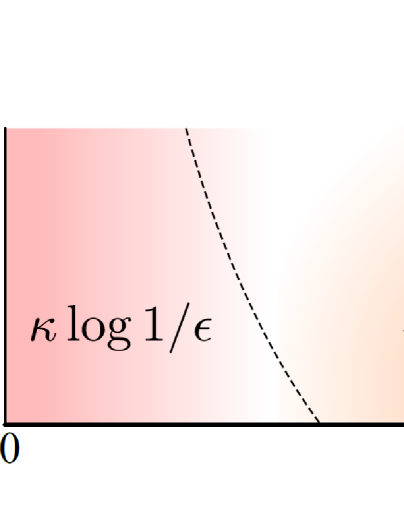
[Corollary 4.3]  [Corollary 4.4]

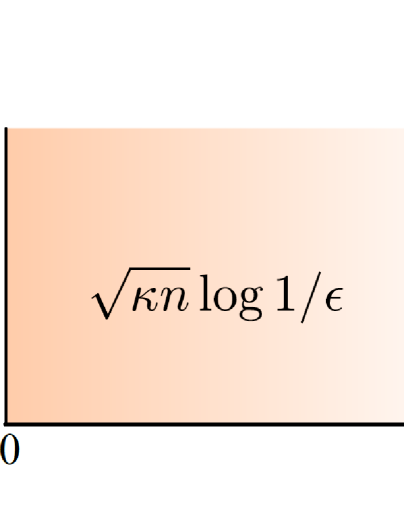
Figure 1: Comparison of the oracle complexities of Algorithm 1 with Option I and Option II.

For the most commonly used uniform random sampling (i.e., sampling probabilities $p_{i}\!=\!1/n$ for all $i\!=\!1,\ldots,n$), the oracle complexity of ASVRG becomes $\mathcal{O}((n\!+\!\!\sqrt{nL/\mu})\log({1}/{\varepsilon}))$, which is identical to that of Katyusha (Allen-Zhu, 2018) and Point-SAGA (Defazio, 2016), and better than those of non-accelerated methods (e.g., $\mathcal{O}\!\left((n\!+\!L/\mu)\log({1}/{\varepsilon})\right)$ of SVRG).

Remark 4.5.

For uniform random sampling, and recalling $L\!=\!L_{\max}\!=\!\max_{j}L_{j}$, the above oracle bound is rewritten as: $\mathcal{O}((n\!+\!\sqrt{nL_{\max}/\mu})\log({1}/{\varepsilon}))$. As each $f_{i}(\cdot)$ generally has different degrees of smoothness $L_{i}$, picking the random index $i_{t}$ from a non-uniform distribution is a much better choice than simple uniform random sampling (Zhao and Zhang, 2015; Needell et al., 2016). For instance, the sampling probabilities for all $f_{i}(\cdot)$ are proportional to their Lipschitz constants, i.e., $p_{i}\!=\!L_{i}/\sum^{n}_{j=1}\!L_{j}$. In this case, the oracle complexity becomes $\mathcal{O}((n\!+\!\sqrt{nL_{\textup{avg}}/\mu})\log({1}/{\varepsilon}))$, where $L_{\textup{avg}}\!=\!\frac{1}{n}\!\sum^{n}_{j=1}\!L_{j}\!\leq\!L_{\max}$. In other words, the statement of Corollary 4.4 can be revised by simply replacing $\widetilde{L}$ with $L_{\textup{avg}}$. And the proof only needs some minor changes accordingly. In fact, all statements in this section can be revised by replacing $\widetilde{L}$ with $L_{\textup{avg}}$.

4.2 Analysis for Non-Strongly Convex Objectives

For non-strongly convex objectives, our second main result is the following theorem, which gives the convergence rate and oracle complexity of Algorithm 2.

Theorem 4.6.

Suppose Assumption 1 holds. Then the following result holds,

$$\begin{split}\mathbb{E}\!\left[F(\widetilde{x}^{S})-F(x^{\star})\right]\leq\frac{4(\alpha\!-\!1)[F(\widetilde{x}^{0})-F(x^{\star})]}{(\alpha-2)^{2}(S+1)^{2}}+\frac{2\|x^{\star}-\widetilde{x}^{0}\|^{2}}{\eta m(S+1)^{2}},\end{split}$$

where $\alpha\!=\!{1}/{(\widetilde{L}\eta)}\!>\!2$. Furthermore, choosing $m\!=\!\Theta(n)$, Algorithm 2 achieves an $\varepsilon$-suboptimal solution, i.e., $\mathbb{E}[F(\widetilde{x}^{S})]-F(x^{\star})\leq\varepsilon$ using at most $\mathcal{O}(\frac{n\sqrt{F(\widetilde{x}^{0})-F(x^{\star})}}{\sqrt{\varepsilon}}+\frac{\sqrt{n\widetilde{L}}\|\widetilde{x}^{0}-x^{\star}\|}{\sqrt{\varepsilon}})$ iterations.

One can see that the oracle complexity of ASVRG is consistent with the best known result in (Hien et al., 2018; Allen-Zhu, 2018), and all the methods attain the optimal convergence rate $\mathcal{O}(1/t^{2})$. Moreover, we can use the adaptive regularization technique in (Allen-Zhu and Hazan, 2016) to the original non-SC problem, and achieve a SC objective $F(x)\!+\!\frac{\sigma_{s}}{2}\|x-\widetilde{x}^{0}\|$ with a decreasing value $\sigma_{s}$, e.g., $\sigma_{s}\!=\!\sigma_{s-1}/2$ in (Allen-Zhu and Hazan, 2016). Then we have the following result.

Corollary 4.7.

Suppose Assumption 1 holds, and $g(\cdot)$ is non-SC. By applying the adaptive regularization technique in (Allen-Zhu and Hazan, 2016) for Algorithm 1, then we obtain an $\varepsilon$-suboptimal solution using at most the following oracle complexity:

$$\mathcal{O}\!\left(n\log\frac{F(\widetilde{x}^{0})-F(x^{\star})}{\varepsilon}+\frac{\sqrt{n\widetilde{L}}\|\widetilde{x}^{0}-x^{\star}\|}{\sqrt{\varepsilon}}\right).$$

Corollary 4.7 implies that ASVRG has a low oracle complexity (i.e., $\mathcal{O}(n\log(1/\varepsilon)\!+\!C_{1}\sqrt{n\widetilde{L}/\varepsilon})$), which is the same as that in (Allen-Zhu, 2018). Both ASVRG and Katyusha have a much faster rate than SAGA (Defazio et al., 2014a), whose oracle complexity is $\mathcal{O}((n\!+\!L)/\varepsilon)$.

Although ASVRG is much simpler than Katyusha, all the theoretical results show that ASVRG achieves the same convergence rates and oracle complexities as Katyusha for both SC and non-SC cases. Similar to (Babanezhad et al., 2015; Allen-Zhu and Yuan, 2016), we can reduce the number of gradient calculations in early iterations to further speed up ASVRG in practice.

5 Extensions of ASVRG

In this section, we first extend ASVRG to the mini-batch setting. Then we extend Algorithm 1 and its convergence results to the non-smooth setting (e.g., the problems in Cases 3 and 4).

5.1 Mini-Batch

In this part, we extend ASVRG and its convergence results to the mini-batch setting. Suppose that the mini-batch size is $b$, the stochastic gradient estimator with variance reduction becomes

$$\widetilde{\nabla}\!f_{I_{t}}\!(x^{s}_{t-1})=\frac{1}{b}\sum_{i\in I_{t}}\!\frac{1}{np_{i}}\!\left[\nabla\!f_{i}(x^{s}_{t-1})-\nabla\!f_{i}(\widetilde{x}^{s-1})\right]+{\nabla}\!f(\widetilde{x}^{s-1}),$$

where $I_{t}\!\subset\![n]$ is a mini-batch of size $b$. Consequently, the momentum parameters $\omega$ and $\omega_{s}$ must satisfy $\omega\!\leq\!1\!-\!\frac{\tau(b)\widetilde{L}\eta}{1-\widetilde{L}\eta}$ and $\omega_{s}\!\leq\!1\!-\!\frac{\tau(b)\widetilde{L}\eta}{1-\widetilde{L}\eta}$ for SC and non-SC cases, respectively, where $\tau(b)\!=\!(n\!-\!b)/[b(n\!-\!1)]$. Moreover, the upper bound on the variance of $\widetilde{\nabla}\!f_{i_{t}}(x^{s}_{t-\!1})$ can be extended to the mini-batch setting as follows.

Lemma 5.1.

$$\begin{split}\mathbb{E}\!\left[\left\|\widetilde{\nabla}\!f_{I_{t}}\!(x^{s}_{t-1})-\nabla\!f(x^{s}_{t-1})\right\|^{2}\right]\leq\frac{2\widetilde{L}(n\!-\!b)}{b(n\!-\!1)}\!\!\left[f(\widetilde{x}^{s-1})\!-\!f(x^{s}_{t-1})\!+\!\nabla\!f(x^{s}_{t-1})^{T}\!(x^{s}_{t-1}\!-\!\widetilde{x}^{s-1})\right]\!.\end{split}$$

In the SC case, the convergence result of the mini-batch variant of ASVRG is identical to Theorem 4.2 and Corollary 4.4. For the non-SC case, we set the initial parameter $\omega_{0}\!=\!1\!-\!\frac{\tau(b)\widetilde{L}\eta}{1-\widetilde{L}\eta}$. Then Theorem 4.6 can be extended to the mini-batch setting as follows.

Theorem 5.2.

Suppose Assumption 1 holds, and given the same notation as in Theorem 4.6 and $\omega_{0}\!=\!1-\frac{\tau(b)\widetilde{L}\eta}{1-\widetilde{L}\eta}$, then the following inequality holds

$$\begin{split}\mathbb{E}\!\left[F(\widetilde{x}^{s})-F(x^{\star})\right]\leq\frac{4(\alpha\!-\!1)\tau(b)[F(\widetilde{x}^{0})\!-\!F(x^{\star})]}{[\alpha-1-\tau(b)]^{2}(s+1)^{2}}+\frac{2\widetilde{L}\alpha\|x^{\star}\!-\!\widetilde{x}^{0}\|^{2}}{m(s+1)^{2}}.\end{split}$$ (8)

Remark 5.3.

For the special case of $b\!=\!1$, we have $\tau(1)\!=\!1$, and then Theorem  5.2 degenerates to Theorem  4.6. When $b\!=\!n$ (i.e., the batch setting), then $\tau(n)\!=\!0$, and the first term on the right-hand side of (8) diminishes. Then our algorithm degenerates to an accelerated deterministic method with the optimal convergence rate of $\mathcal{O}(1/t^{2})$, where $t$ is the number of iterations.

5.2 Non-Smooth Settings

In addition to the application of the regularization reduction technique in (Allen-Zhu and Hazan, 2016) for a class of smooth and non-SC problems (i.e., Case 2 of Problem (1)), as shown in Section 4.2, ASVRG can also be extended to solve the problems in both Cases 3 and 4, when each component of $f$ is $G$-Lipschitz continuous, which is defined as follows.

Definition 5.4.

The function $f_{i}(x)$ is $G$-Lipschitz continuous if there exists a constant $G$ such that, for any $x,y\!\in\!\mathbb{R}^{d}$, $|f_{i}(x)-f_{i}(y)|\leq G\|x-y\|$.

The key technique is using a proximal operator to obtain gradients of the $\delta_{s}$-Moreau envelope of a non-smooth function $f_{i}(\cdot)$, defined as

$$f^{\delta_{s}}_{i}(x)=\inf_{y\in\mathbb{R}^{d}}f_{i}(y)+\frac{\delta_{s}}{2}\|x-y\|^{2},$$ (9)

where $\delta_{s}$ is an increasing parameter as in (Allen-Zhu and Hazan, 2016). That is, we use the proximal operator to smoothen each component function, and optimize the new, smooth function which approximates the original problem. This technique has been used in Katyusha (Allen-Zhu, 2018) and accelerated SDCA (Shalev-Shwartz and Zhang, 2016) for non-smooth objectives.

Property 1 (Nesterov (2005); Bauschke and Combettes (2011); Orabona et al. (2012))

Let each $f_{i}(x)$ be convex and $G$-Lipschitz continuous. For any $\delta>0$, the following results hold:
(a) $f^{\delta}_{i}(x)$ is $\delta$-smooth;
(b) $\nabla(f^{\delta}_{i})(x)=\delta\!\left(x-\textup{prox}^{\,f_{i}}_{\delta}(x)\right)$;
(c) $f^{\delta}_{i}(x)\leq f_{i}(x)\leq f^{\delta}_{i}(x)+\frac{G^{2}}{2\delta}$.

By using the similar techniques in (Allen-Zhu and Hazan, 2016), we can apply ASVRG to solve the smooth problem $F^{\delta_{s}}(x)\!:=\!\frac{1}{n}\!\sum^{n}_{i=1}\!f^{\delta_{s}}_{i}(x)\!+\!g(x)$. It is easy to verify that ASVRG satisfies the homogenous objective decrease (HOOD) property in (Allen-Zhu and Hazan, 2016) (see (Allen-Zhu and Hazan, 2016) for the detail of HOOD), as shown below.

Corollary 5.5.

Algorithm 1 used to solve the problem in Case 1 satisfies the HOOD property with at most $\mathcal{O}(n\!+\!\sqrt{n\widetilde{L}/\mu})$ iterations. That is, for every starting point $\widetilde{x}^{0}$, Algorithm 1 produces an output $\widetilde{x}^{s}$ satisfying $\mathbb{E}\!\left[F(\widetilde{x}^{s})\right]\!-\!F(x^{\star})\!\leq\![F(\widetilde{x}^{0})\!-\!F(x^{\star})]/4$ in at most $\mathcal{O}(n\!+\!\sqrt{n\widetilde{L}/\mu})$ iterations.

In the following, we extend the result in Theorem 4.2 to the non-smooth setting as follows.

Corollary 5.6.

Let $f_{i}(x)$ be $G$-Lpischitz continuous, and $g(x)$ be $\mu$-strongly convex. By applying the adaptive smooth technique in (Allen-Zhu and Hazan, 2016) on ASVRG, we obtain an $\varepsilon$-suboptimal solution using at most the following oracle complexity:

$$\mathcal{O}\!\left(n\log\frac{F(\widetilde{x}^{0})-F(x^{\star})}{\varepsilon}+\frac{\sqrt{n}G}{\sqrt{\mu\varepsilon}}\right).$$

Corollary 5.7.

Let $f_{i}(x)$ be $G$-Lpischitz continuous and $g(x)$ be not necessarily strongly convex. By applying both the adaptive regularization and smooth techniques in (Allen-Zhu and Hazan, 2016) on ASVRG, we obtain an $\varepsilon$-suboptimal solution using at most the following oracle complexity:

$$\mathcal{O}\!\left(n\log\frac{F(\widetilde{x}^{0})-F(x^{\star})}{\varepsilon}+\frac{\sqrt{n}G\|\widetilde{x}^{0}-x^{\star}\|}{\varepsilon}\right).$$

From Corollaries 5.6 and 5.7, one can see that ASVRG converges to an $\varepsilon$-accurate solution for Case 3 of Problem (1) in $\mathcal{O}\!\left(n\log\frac{C_{2}}{\varepsilon}\!+\!\!\frac{\sqrt{n}G}{\sqrt{\mu\varepsilon}}\right)$ iterations and for Case 4 in $\mathcal{O}\!\left(n\log\frac{C_{2}}{\varepsilon}\!+\!\!\frac{\sqrt{n}C_{1}G}{\varepsilon}\right)$ iterations. That is, ASVRG achieves the same low oracle complexities as the accelerated stochastic variance reduction method, Katyusha, for the two classes of non-smooth problems (i.e., Cases 3 and 4 of Problem (1)).

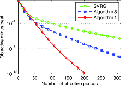
[RCV1,  $\lambda=10^{-6}$]     [Covtype,  $\lambda=10^{-7}$]

Figure 2: Comparison of SVRG Johnson and Zhang (2013), ASVRG without momentum (i.e., Algorithm 3), and ASVRG (i.e., Algorithm 1) for ridge regression.

6 Experiments

In this section, we evaluate the performance of ASVRG, and all the experiments were performed on a PC with an Intel i5-2400 CPU and 16GB RAM. We used the two publicly available data sets in our experiments: Covtype and RCV1, which can be downloaded from the LIBSVM Data website.

6.1 Effectiveness of Our Momentum

Figure 2 shows the performance of ASVRG with $\theta_{s}\!\equiv\!1$ (i.e., Algorithm 3) and ASVRG in order to illustrate the importance and effectiveness of our momentum. Note that the epoch length is set to $m\!=\!2n$ for the two algorithms (i.e., $m_{1}\!=\!2n$ and $\rho\!=\!1$), as well as SVRG (Johnson and Zhang, 2013). It is clear that Algorithm 3 is without our momentum acceleration technique. The main difference between Algorithm 3 and SVRG is that the snapshot and starting points of the former are set to the uniform average and last iterate of the previous epoch, respectively, while the two points of the later are the last iterate. The results show that Algorithm 3 outperforms SVRG, suggesting that the iterate average can work better in practice, as discussed in (Shang et al., 2018b). In particular, ASVRG converges significantly faster than ASVRG without momentum and SVRG, meaning that our momentum acceleration technique can accelerate the convergence of ASVRG.

6.2 Comparison with Stochastic Methods

For fair comparison, ASVRG and the compared algorithms (including SVRG (Johnson and Zhang, 2013), SAGA (Defazio et al., 2014a), Acc-Prox-SVRG (Nitanda, 2014), Catalyst (Lin et al., 2015), and Katyusha (Allen-Zhu, 2018)) were implemented in C++ with a Matlab interface. There is only one parameter (i.e., the learning rate) to tune for all these methods except Catalyst and Acc-Prox-SVRG. In particular, we compare their performance in terms of both the number of effective passes over the data and running time (seconds). As in (Xiao and Zhang, 2014), each feature vector has been normalized so that it has norm $1$.

Figure 3 shows how the objective gap (i.e., $F(x^{s})\!-\!F(x^{\star})$) of all these methods decreases on elastic net regularized logistic regression ($\lambda_{1}\!=\!10^{-4}$, $\lambda_{2}\!=\!10^{-5}$) as time goes on. It is clear that ASVRG converges significantly faster than the other methods in terms of both oracle calls and running time, while Catalyst and Katyusha achieve comparable and sometimes even better performance than SVRG and SAGA in terms of the running time (seconds). The main reason is that ASVRG not only takes advantage of the momentum acceleration trick, but also can use much larger step-size (e.g., 1/(3$L$) for ASVRG vs. 1/(10$L$) for SVRG). This empirically verifies our theoretical result in Corollary 4.4 that ASVRG has the same low oracle complexity as Katyusha. ASVRG significantly outperforms Katyusha in terms of running time, which implies that ASVRG has a much lower per-iteration cost than Katyusha.

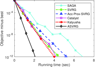
Figure 3: Comparison of SAGA (Defazio et al., 2014a), SVRG (Johnson and Zhang, 2013), Acc-Prox-SVRG (Nitanda, 2014), Catalyst (Lin et al., 2015), Katyusha (Allen-Zhu, 2018) and ASVRG on Covtype.

7 Conclusions

We proposed an efficient ASVRG method, which integrates both the momentum acceleration trick and variance reduction technique. We first designed a simple momentum acceleration technique. Then we theoretically analyzed the convergence properties of ASVRG, which show that ASVRG achieves the same low oracle complexities for both SC and non-SC objectives as accelerated methods, e.g., Katyusha (Allen-Zhu, 2018). Moreover, we also extended ASVRG and its convergence results to both mini-batch settings and non-smooth settings.

It would be interesting to consider other classes of settings, e.g., the non-Euclidean norm setting. In practice, ASVRG is much simpler than the existing accelerated methods, and usually converges much faster than them, which has been verified in our experiments. Due to its simplicity, it is more friendly to asynchronous parallel and distributed implementation for large-scale machine learning problems (Zhou et al., 2018), similar to (Reddi et al., 2015; Sra et al., 2016; Mania et al., 2017; Zhou et al., 2018; Lee et al., 2017; Wang et al., 2017). One natural open problem is whether the best oracle complexities can be obtained by ASVRG in the asynchronous and distributed settings.

Acknowledgments

We thank the reviewers for their valuable comments. This work was supported in part by Grants (CUHK 14206715 & 14222816) from the Hong Kong RGC, Project supported the Foundation for Innovative Research Groups of the National Natural Science Foundation of China (No. 61621005), the Major Research Plan of the National Natural Science Foundation of China (Nos. 91438201 and 91438103), the National Natural Science Foundation of China (Nos. 61876220, 61876221, 61836009, U1701267, 61871310, 61573267, 61502369 and 61473215), the Program for Cheung Kong Scholars and Innovative Research Team in University (No. IRT_15R53), the Fund for Foreign Scholars in University Research and Teaching Programs (the 111 Project) (No. B07048), and the Science Foundation of Xidian University (No. 10251180018).

In this supplementary material, we give the detailed proofs for some lemmas, theorems and properties.

Appendix A

Appendix A1: Proof of Proposition 1

Proof A.1.

Using Theorem 1, we have

$$\rho(\omega)=1-\omega+\frac{\omega^{2}}{\mu m\eta}.$$

Obviously, it is desirable to have a small convergence factor $\rho(\omega)$. So, we minimize $\rho(\omega)$ with given $\eta$. Then we have

$$\omega_{\star}=m\mu\eta/2\leq 1-\frac{\widetilde{L}\eta}{1-\widetilde{L}\eta},$$

and

$$\rho(\omega_{\star})=1-\frac{m\mu\eta}{4}>0.$$

The above two inequalities imply that

$$\eta\leq\frac{1+4c_{1}-\sqrt{1+16c_{1}^{2}}}{2\widetilde{L}}=\frac{1+4c_{1}-\sqrt{1+16c_{1}^{2}}}{2c_{1}m\mu}\quad\textrm{and}\quad\eta<\frac{4}{m\mu},$$

where $c_{1}={\widetilde{L}}/{(m\mu)}>0$. This completes the proof.

Appendix A2: ASVRG Pseudo-Codes

We first give the details on Algorithm 1 with $\omega\!=\!1$ for optimizing smooth objective functions such as $\ell_{2}$-norm regularized logistic regression, as shown in Algorithm 3, which is almost identical to the regularized SVRG in (Babanezhad et al., 2015) and the original SVRG in (Johnson and Zhang, 2013). The main differences between Algorithm 3 and the latter two are the initialization of $x^{s}_{0}$ and the choice of the snapshot point $\widetilde{x}^{s}$. Moreover, we can use the doubling-epoch technique in (Mahdavi et al., 2013; Allen-Zhu and Yuan, 2016) to further speed up our ASVRG method for both SC and non-SC cases. Besides, all the proposed algorithms can be extended to the mini-batch setting as in (Nitanda, 2014; Konečný et al., 2016). In particular, our ASVRG method can be extended to an accelerated incremental aggregated gradient method with the SAGA estimator in (Defazio et al., 2014a).

Algorithm 3 ASVRG with $\omega=1$

0:  The number of epochs $S$, the number of iterations $m$ per epoch, and the step size $\eta$.

0:  $x^{1}_{0}=\widetilde{x}^{0}$, $m_{1}=n/4$, $\rho>1$, and the probability $P=[p_{1},\ldots,p_{n}]$.

1:  for $s=1,2,\ldots,S$ do

2:     $\widetilde{\nabla}=\frac{1}{n}\!\sum^{n}_{i=1}\!\nabla\!f_{i}(\widetilde{x}^{s-1})$;

3:     for $t=1,2,\ldots,m_{s}$ do

4:        Pick $i_{t}$ from $\{1,\ldots,n\}$ randomly based on $P$;

5:        $\widetilde{\nabla}\!f_{i_{t}}(x^{s}_{t-1})=\left[\nabla\!f_{i_{t}}(x^{s}_{t-1})-\nabla\!f_{i_{t}}(\widetilde{x}^{s-1})\right]/(np_{i_{t}})+\widetilde{\nabla}$;

6:        $x^{s}_{t}=x^{s}_{t-1}-\eta\left[\widetilde{\nabla}\!f_{i_{t}}(x^{s}_{t-1})+\nabla\!g(x^{s}_{t-1})\right]$;

7:     end for

8:     $\widetilde{x}^{s}=\frac{1}{m_{s}}\!\sum^{m_{s}}_{t=1}\!x^{s}_{t}$,  $x^{s+1}_{0}=x^{s}_{m_{s}}$,  $m_{s+1}=\min(\lfloor\rho m_{s}\rfloor,m)$;

9:  end for

9:  $\widetilde{x}^{S}$.

Appendix A3: Elastic-Net Regularized Logistic Regression

In this paper, we mainly focus on the following elastic-net regularized logistic regression problem for binary classification,

$$\min_{x\in\mathbb{R}^{d}}\frac{1}{n}\sum^{n}_{i=1}\log(1+\exp(-b_{i}a^{T}_{i}x))+\frac{\lambda_{1}}{2}\|x\|^{2}+\lambda_{2}\|x\|_{1},$$

where $\{(a_{i},b_{i})\}$ is a set of training examples, and $\lambda_{1},\lambda_{2}\!\geq\!0$ are the regularization parameters. Note that $f_{i}(x)\!=\!\log(1\!+\!\exp(-b_{i}a^{T}_{i}x))\!+\!(\lambda_{1}/{2})\|x\|^{2}$.

In this paper, we used the two publicly available data sets in the experiments: Covtype and RCV1, as listed in Table 2. For fair comparison, we implemented the state-of-the-art stochastic methods such as SAGA (Defazio et al., 2014a), SVRG (Johnson and Zhang, 2013), Acc-Prox-SVRG (Nitanda, 2014), Catalyst (Lin et al., 2015), and Katyusha (Allen-Zhu, 2018), and our ASVRG method in C++ with a Matlab interface, and conducted all the experiments on a PC with an Intel i5-4570 CPU and 16GB RAM.

Table 2: Summary of data sets used for our experiments.

Data sets	Covtype	RCV1
Number of training samples, $n$	581,012	20,242
Number of dimensions, $d$	54	47,236
Sparsity	22.12%	0.16%
Size	50M	13M

Appendix B Proof of Lemma 2

Before proving the key Lemma 2, we first give the following lemma and properties, which are useful for the convergence analysis of our ASVRG method.

Lemma B.1.

Suppose Assumption 1 holds. Then the following inequality holds

$$\begin{split}&\mathbb{E}\!\left[\left\|\widetilde{\nabla}\!f_{i_{t}}\!(x^{s}_{t-1})-\nabla\!f(x^{s}_{t-1})\right\|^{2}\right]\leq\,2\widetilde{L}\!\left(f(\widetilde{x}^{s-1})-f(x^{s}_{t-1})+\left\langle\nabla\!f(x^{s}_{t-1}),\;x^{s}_{t-1}-\widetilde{x}^{s-1}\right\rangle\right)\!,\end{split}$$ (10)

where $\langle\cdot,\cdot\rangle$ denotes the inner product (i.e., $\langle x,y\rangle\!=\!x^{T}y$ for all $x,y\!\in\!\mathbb{R}^{d}$), and $\widetilde{L}\!=\!\max_{j}L_{j}/(p_{j}n)$. When $p_{i}\!=\!1/n$ (i.e., uniform random sampling), $\widetilde{L}\!=\!L_{\max}\!:=\!\max_{j}L_{j}$, while $\widetilde{L}\!=\!L_{\textup{avg}}\!:=\!\frac{1}{n}\!\sum^{n}_{j=1}\!L_{j}$ when $p_{i}\!=\!L_{i}/\sum^{n}_{j=1}\!L_{j}$ (i.e., the sampling probabilities $p_{i}$ for $i\!\in\!\{1,\ldots,n\}$ are proportional to their Lipschitz constants $L_{i}$ of ${\nabla}\!f_{i}(\cdot)$).

The proof of Lemma B.1 is similar to that of Lemma 3.4 in (Allen-Zhu, 2018). For the sake of completeness, we give the detailed proof of Lemma B.1 as follows. Their main difference is that Lemma B.1 provides the upper bound on the expected variance of the modified stochastic gradient estimator, i.e.,

$$\widetilde{\nabla}\!f_{i_{t}}\!(x^{s}_{t-1})=\left[\nabla\!f_{i_{t}}\!(x^{s}_{t-1})-\nabla\!f_{i_{t}}\!(\widetilde{x}^{s-1})\right]\!/(np_{i_{t}})+\widetilde{\nabla},$$

while the upper bound in Lemma 3.4 in (Allen-Zhu, 2018) is for the standard stochastic gradient estimator in (Johnson and Zhang, 2013; Zhang et al., 2013). Obviously, the upper bound in Lemma B.1 is much tighter than that in (Johnson and Zhang, 2013; Xiao and Zhang, 2014; Allen-Zhu and Yuan, 2016), e.g., Corollary 3.5 in (Xiao and Zhang, 2014) and Lemma A.2 in (Allen-Zhu and Yuan, 2016).

Proof B.2.

Now we take expectations with respect to the random choice of $i_{t}$, to obtain

$$\begin{split}&\;\mathbb{E}\!\left[\frac{1}{np_{i_{t}}}\!\left[\nabla\!f_{i_{t}}(x^{s}_{t-1})-\nabla\!f_{i_{t}}(\widetilde{x}^{s-1})\right]\right]\\ =&\;\sum^{n}_{i=1}\frac{p_{i}}{np_{i}}\!\left[\nabla\!f_{i}(x^{s}_{t-1})-\nabla\!f_{i}(\widetilde{x}^{s-1})\right]\\ =&\;\sum^{n}_{i=1}\frac{1}{n}\left[\nabla\!f_{i}(x^{s}_{t-1})-\nabla\!f_{i}(\widetilde{x}^{s-1})\right]\\ =&\;\nabla\!f(x^{s}_{t-1})-\nabla\!f(\widetilde{x}^{s-1}).\end{split}$$ (11)

Theorem 2.1.5 in (Nesterov, 2004) immediately implies the following result.

$$\begin{split}&\left\|\nabla\!f_{i}(x^{s}_{t-1})-\nabla\!f_{i}(\widetilde{x}^{s-1})\right\|^{2}\leq 2L_{i}\!\left[f_{i}(\widetilde{x}^{s-1})-f_{i}(x^{s}_{t-1})+\langle\nabla\!f_{i}(x^{s}_{t-1}),\;x^{s}_{t-1}-\widetilde{x}^{s-1}\rangle\right]\!.\end{split}$$

Dividing both sides of the above inequality by $1/(n^{2}p_{i})$, and summing it over $i\!=\!1,\ldots,n$, we obtain

$$\begin{split}&\;\frac{1}{n}\sum^{n}_{i=1}\frac{1}{np_{i}}\left\|\nabla\!f_{i}(x^{s}_{t-1})-\nabla\!f_{i}(\widetilde{x}^{s-1})\right\|^{2}\\ \leq&\;2\widetilde{L}\!\left[f(\widetilde{x}^{s-\!1})-f(x^{s}_{t-1})+\langle\nabla\!f(x^{s}_{t-1}),\;x^{s}_{t-1}-\widetilde{x}^{s-1}\rangle\right]\!.\end{split}$$ (12)

Using the definition of $\widetilde{\nabla}\!f_{i_{t}}(x^{s}_{t-1})=[\nabla\!f_{i_{t}}(x^{s}_{t-1})-\nabla\!f_{i_{t}}(\widetilde{x}^{s-1})]/(np_{i_{t}})+\nabla\!f(\widetilde{x}^{s-1})$, (11), and (12), we have

$$\begin{split}&\;\mathbb{E}\!\left[\left\|\widetilde{\nabla}\!f_{i_{t}}\!(x^{s}_{t-1})-\nabla\!f(x^{s}_{t-1})\right\|^{2}\right]\\ =&\;\mathbb{E}\!\left[\left\|\nabla\!f(\widetilde{x}^{s-1})-\nabla\!f(x^{s}_{t-1})-\frac{\nabla\!f_{i_{t}}\!(\widetilde{x}^{s-1})-\nabla\!f_{i_{t}}\!(x^{s}_{t-1})}{np_{i_{t}}}\right\|^{2}\right]\\ \leq&\;\mathbb{E}\!\left[\frac{1}{n^{2}p^{2}_{i_{t}}}\!\left\|\nabla\!f_{i_{t}}\!(x^{s}_{t-1})-\nabla\!f_{i_{t}}\!(\widetilde{x}^{s-1})\right\|^{2}\right]\\ =&\;\frac{1}{n}\sum^{n}_{i=1}\frac{1}{np_{i}}\left\|\nabla\!f_{i}(x^{s}_{t-1})-\nabla\!f_{i}(\widetilde{x}^{s-1})\right\|^{2}\\ \leq&\;2\widetilde{L}\left[f(\widetilde{x}^{s-1})-f(x^{s}_{t-1})+\langle\nabla\!f(x^{s}_{t-1}),\;x^{s}_{t-1}-\widetilde{x}^{s-1}\rangle\right]\!,\end{split}$$

where the first inequality follows from the fact that $\mathbb{E}[\|\mathbb{E}[x]-x\|^{2}]=\mathbb{E}[\|x\|^{2}]-\|\mathbb{E}[x]\|^{2}\leq\mathbb{E}[\|x\|^{2}]$, and the second inequality holds due to (12).

Property 2 (Lan (2012))

Assume that $z^{*}$ is an optimal solution of the following problem,

$$\min_{z}\frac{\nu}{2}\|z-z_{0}\|^{2}+h(z),$$

where $h(z)$ is a convex function (but possibly non-differentiable). Then for any $z\!\in\!\mathbb{R}^{d}$,

$$h(z^{*})+\frac{\nu}{2}\|z^{*}-z_{0}\|^{2}+\frac{\nu}{2}\|z-z^{*}\|^{2}\leq h(z)+\frac{\nu}{2}\|z-z_{0}\|^{2}.$$

Property 3

Assume that the stochastic momentum weight $\omega_{s}$ in Algorithm 2 satisfies the following conditions:

$$\omega_{0}\leq 1-\frac{1}{\alpha-1}\;\;\textup{and}\;\;\frac{1-\omega_{s}}{\omega^{2}_{s}}=\frac{1}{\omega^{2}_{s-1}},$$ (13)

where $\alpha=1/(\widetilde{L}\eta)$. Then the following properties hold:

$$\begin{split}\omega_{s}=\frac{\sqrt{\omega^{4}_{s-1}+4\omega^{2}_{s-1}}-\omega^{2}_{s-1}}{2},\quad\omega_{s}\leq\frac{2}{s+2}.\end{split}$$

Proof B.3.

Using the equality in (13), it is easy to show that

$$\omega_{s}=\frac{\sqrt{\omega^{4}_{s-1}+4\omega^{2}_{s-1}}-\omega^{2}_{s-1}}{2}\geq 0.$$

In the following, we will prove by induction that $\omega_{s}\leq\frac{2}{s+2}$. Firstly, we have

$$\omega_{0}\leq 1-\frac{1}{\alpha-1}\leq 1=\frac{2}{0+2}.$$

Assume that $\omega_{s-1}\leq\frac{2}{s+1}$, then we have

$$\begin{split}\omega_{s}&=\frac{\sqrt{\omega^{4}_{s-1}+4\omega^{2}_{s-1}}-\omega^{2}_{s-1}}{2}=\frac{2}{1+\sqrt{1+\frac{4}{\omega^{2}_{s-1}}}}\\ &\leq\frac{2}{1+\sqrt{1+(s+1)^{2}}}\\ &\leq\frac{2}{s+2}.\end{split}$$

This completes the proof.

Proof of Lemma 2:

Proof B.4.

Let $\widetilde{\nabla}_{t}:=\!\left[\nabla f_{i_{t}}\!(x^{s}_{t-1})-\nabla f_{i_{t}}\!(\widetilde{x}^{s-1})\right]/(np_{i_{t}})+\nabla f(\widetilde{x}^{s-1})$. Suppose each component function $f_{i}(\cdot)$ is $L_{i}$-smooth, which implies that the gradient of the average function $f(x)$ is convex and also Lipschitz-continuous, i.e., there exists a Lipschitz constant $L_{f}\!>0$ such that for all $x,y\!\in\!\mathbb{R}^{d}$,

$$\|\nabla f(x)-\nabla f(y)\|\leq L_{f}\|x-y\|,$$

whose equivalent form is

$$f(y)\leq f(x)+\langle\nabla f(x),\;y-x\rangle+\frac{L_{f}}{2}\|y-x\|^{2}.$$

Moreover, it is easy to verify that $L_{f}\leq L_{\textup{avg}}=\frac{1}{n}\sum^{n}_{j=1}L_{j}\leq\widetilde{L}$. Let $\eta=1/(\widetilde{L}\alpha)$ and $\alpha>2$ be a suitable constant, then we have

$$\begin{split}f(x^{s}_{t})\leq\,&f(x^{s}_{t-1})+\left\langle\nabla f(x^{s}_{t-1}),\,x^{s}_{t}-x^{s}_{t-1}\right\rangle+\frac{L_{f}}{2}\!\left\|x^{s}_{t}-x^{s}_{t-1}\right\|^{2}\\ \leq\,&f(x^{s}_{t-1})+\left\langle\nabla f(x^{s}_{t-1}),\,x^{s}_{t}-x^{s}_{t-1}\right\rangle+\frac{\widetilde{L}}{2}\!\left\|x^{s}_{t}-x^{s}_{t-1}\right\|^{2}\\ =\,&f(x^{s}_{t-1})+\left\langle\nabla f(x^{s}_{t-1}),\,x^{s}_{t}-x^{s}_{t-1}\right\rangle+\frac{\widetilde{L}\alpha}{2}\!\left\|x^{s}_{t}-x^{s}_{t-1}\right\|^{2}-\frac{\widetilde{L}(\alpha\!-\!1)}{2}\!\left\|x^{s}_{t}-x^{s}_{t-1}\right\|^{2}\\ =\,&f(x^{s}_{t-1})+\left\langle\widetilde{\nabla}_{{t}},\,x^{s}_{t}-x^{s}_{t-1}\right\rangle+\frac{\widetilde{L}\alpha}{2}\|x^{s}_{t}-x^{s}_{t-1}\|^{2}-\frac{\widetilde{L}(\alpha\!-\!1)}{2}\|x^{s}_{t}-x^{s}_{t-1}\|^{2}\\ &+\left\langle\nabla f(x^{s}_{t-1})-\widetilde{\nabla}_{{t}},\,x^{s}_{t}-x^{s}_{t-1}\right\rangle.\end{split}$$ (14)

$$\begin{split}&\mathbb{E}\!\left[\left\langle\nabla\!f(x^{s}_{t-1})-\widetilde{\nabla}_{{t}},\,x^{s}_{t}-x^{s}_{t-1}\right\rangle\right]\\ \leq\,&\mathbb{E}\!\left[\frac{1}{2\widetilde{L}(\alpha\!-\!1)}\left\|\nabla\!f(x^{s}_{t-1})-\widetilde{\nabla}_{{t}}\right\|^{2}+\frac{\widetilde{L}(\alpha\!-\!1)}{2}\left\|x^{s}_{t}\!-\!x^{s}_{t-1}\right\|^{2}\right]\\ \leq\,&\frac{1}{\alpha\!-\!1}\!\left[f(\widetilde{x}^{s-1})-f(x^{s}_{t-1})+\left\langle\nabla f(x^{s}_{t-1}),\;x^{s}_{t-1}-\widetilde{x}^{s-1}\right\rangle\right]+\frac{\widetilde{L}(\alpha\!-\!1)}{2}\mathbb{E}\!\left[\left\|x^{s}_{t}\!-\!x^{s}_{t-1}\right\|^{2}\right],\end{split}$$ (15)

where the first inequality holds due to the Young’s inequality, i.e., $a^{T}b\!\leq\!{\|a\|^{2}}/{(2\theta)}\!+\!{\theta\|b\|^{2}}/{2}$ for all $\theta\!>\!0$, and the second inequality follows from Lemma B.1.

Taking the expectation over the random choice of $i_{t}$, and substituting the inequality (15) into the inequality (14), then we have

$$\begin{split}\mathbb{E}[F(x^{s}_{t})]&\leq f(x^{s}_{t-1})+\mathbb{E}\!\left[\left\langle\widetilde{\nabla}_{{t}},\,x^{s}_{t}-x^{s}_{t-1}\right\rangle+\frac{\widetilde{L}\alpha}{2}\|x^{s}_{t}-x^{s}_{t-1}\|^{2}+g(x^{s}_{t})\right]\\ &\quad+\frac{1}{\alpha\!-\!1}\!\left[f(\widetilde{x}^{s-1})-f(x^{s}_{t-1})+\left\langle\nabla f(x^{s}_{t-1}),\;x^{s}_{t-1}-\widetilde{x}^{s-1}\right\rangle\right]\\ &\leq f(x^{s}_{t-1})+\mathbb{E}\!\left[\omega_{s-1}\left\langle\widetilde{\nabla}_{t},\,y^{s}_{t}-y^{s}_{t-1}\right\rangle+\frac{\widetilde{L}\alpha\omega^{2}_{s-1}}{2}\|y^{s}_{t}-y^{s}_{t-1}\|^{2}+\omega_{s-1}g(y^{s}_{t})\right]\\ &\quad+(1-\omega_{s-1})g(\widetilde{x}^{s-1})+\frac{1}{\alpha\!-\!1}\!\left[f(\widetilde{x}^{s-1})-f(x^{s}_{t-1})+\left\langle\nabla f(x^{s}_{t-1}),\;x^{s}_{t-1}-\widetilde{x}^{s-1}\right\rangle\right]\\ &\leq\!f(x^{s}_{t-\!1})\!+\!\mathbb{E}\!\left[\omega_{s-\!1}\!\left\langle\!\widetilde{\nabla}_{\!t},\,x^{\star}\!\!-\!y^{s}_{t-\!1}\right\rangle\!+\!\frac{\widetilde{L}\alpha\omega^{2}_{s-\!1}}{2}(\|x^{\star}\!\!-\!y^{s}_{t-\!1}\|^{2}\!-\!\|x^{\star}\!\!-\!y^{s}_{t}\|^{2})\!+\!\omega_{s-\!1}g(x^{\star})\right]\\ &\quad+(1-\omega_{s-1})g(\widetilde{x}^{s-1})+\frac{1}{\alpha\!-\!1}\!\left[f(\widetilde{x}^{s-1})-f(x^{s}_{t-1})+\left\langle\nabla f(x^{s}_{t-1}),\;x^{s}_{t-1}-\widetilde{x}^{s-1}\right\rangle\right]\\ &=f(x^{s}_{t-\!1})+\mathbb{E}\!\left[\frac{\widetilde{L}\alpha\omega^{2}_{s-\!1}}{2}\!\left(\|x^{\star}\!-\!y^{s}_{t-1}\|^{2}\!-\!\|x^{\star}\!-\!y^{s}_{t}\|^{2}\right)\!+\!\omega_{s-1}g(x^{\star})\right]\!+\!(1\!-\!\omega_{s-\!1})g(\widetilde{x}^{s-\!1})\\ &\quad+\left\langle\nabla f(x^{s}_{t-\!1}),\;\omega_{s-1}x^{\star}+(1-\omega_{s-1})\widetilde{x}^{s-1}\!-\!x^{s}_{t-\!1}\!+\!\frac{1}{\alpha\!-\!1}(x^{s}_{t-\!1}\!-\!\widetilde{x}^{s-\!1})\right\rangle\\ &\quad+\!\mathbb{E}\!\left[\left\langle-\!\nabla\!f_{i_{t}}\!(\widetilde{x}^{s-\!1})\!+\!\nabla\!f(\widetilde{x}^{s-\!1}),\;\omega_{s-\!1}x^{\star}\!\!+\!(1\!-\!\omega_{s-\!1})\widetilde{x}^{s-1}\!\!-\!x^{s}_{t-\!1}\right\rangle\right]\!+\!\frac{f(\widetilde{x}^{s-\!1})\!-\!f(x^{s}_{t-\!1})}{\alpha\!-\!1}\\ &=f(x^{s}_{t-\!1})\!+\!\mathbb{E}\!\left[\frac{\widetilde{L}\alpha\omega^{2}_{s-\!1}}{2}\!\left(\|x^{\star}\!-\!y^{s}_{t-1}\|^{2}\!-\!\|x^{\star}\!-\!y^{s}_{t}\|^{2}\right)\!+\!\omega_{s-\!1}g(x^{\star})\right]\!+\!(1\!-\!\omega_{s-\!1})g(\widetilde{x}^{s-\!1})\\ &\quad+\left\langle\nabla f(x^{s}_{t-\!1}),\;\omega_{s-1}x^{\star}+(1-\omega_{s-1})\widetilde{x}^{s-1}\!-\!x^{s}_{t-\!1}\!+\!\frac{1}{\alpha\!-\!1}(x^{s}_{t-\!1}\!-\!\widetilde{x}^{s-\!1})\right\rangle\\ &\quad+\frac{1}{\alpha\!-\!1}\left(f(\widetilde{x}^{s-1})-f(x^{s}_{t-1})\right),\end{split}$$ (16)

where the first inequality holds due to the inequalities (14) and (15); the second inequality follows from the facts that $x^{s}_{t}=\widetilde{x}^{s-1}+\omega_{s-1}(y^{s}_{t}-\widetilde{x}^{s-1})=\omega_{s-1}y^{s}_{t}+(1-\omega_{s-1})\widetilde{x}^{s-1}$, $x^{s}_{t}-x^{s}_{t-1}=\omega_{s-1}(y^{s}_{t}-y^{s}_{t-1})$, and

$$g(\omega_{s-1}y^{s}_{t}+(1-\omega_{s-1})\widetilde{x}^{s-1})\leq\omega_{s-1}g(y^{s}_{t})+(1-\omega_{s-1})g(\widetilde{x}^{s-1}).$$

Since $y^{s}_{t}$ is the optimal solution of the problem (5), the third inequality follows from Property 2 with $z^{*}=y^{s}_{t}$, $z=x^{\star}$, $z_{0}=y^{s}_{t-1}$, $\nu=\widetilde{L}\alpha\omega_{s-1}={\omega_{s-\!1}}/{\eta}$ and $h(y):=\langle\widetilde{\nabla}_{{t}},\,y-y^{s}_{t-1}\rangle+g(y)$. The first equality holds due to the facts that

$$\begin{split}&\;\omega_{s-1}\left\langle\widetilde{\nabla}_{{t}},\;x^{\star}-y^{s}_{t-1}\right\rangle\\ =&\;\left\langle\widetilde{\nabla}_{{t}},\;\omega_{s-1}x^{\star}+(1-\omega_{s-1})\widetilde{x}^{s-1}-x^{s}_{t-1}\right\rangle\\ =&\;\left\langle\nabla\!f_{i_{t}}\!(x^{s}_{t-\!1}),\;\omega_{s-\!1}x^{\star}\!+\!(1\!-\!\omega_{s-\!1})\widetilde{x}^{s-\!1}\!-\!x^{s}_{t-\!1}\right\rangle\\ &\;+\left\langle-\nabla\!f_{i_{t}}\!(\widetilde{x}^{s-\!1})\!+\!\nabla\!f(\widetilde{x}^{s-\!1}),\;\omega_{s-\!1}x^{\star}\!+\!(1\!-\!\omega_{s-\!1})\widetilde{x}^{s-\!1}\!-\!x^{s}_{t-\!1}\right\rangle,\end{split}$$

and $\mathbb{E}[\nabla\!f_{i_{t}}(x^{s}_{t-1})]=\nabla\!f(x^{s}_{t-1})$, and the last equality follows from the fact that

$$\mathbb{E}\left[\langle-\nabla\!f_{i_{t}}(\widetilde{x}^{s-1})+\nabla\!f(\widetilde{x}^{s-1}),\,\omega_{s-1}x^{\star}+(1-\omega_{s-1})\widetilde{x}^{s-1}-x^{s}_{t-1}\rangle\right]=0.$$

Furthermore,

$$\begin{split}&\left\langle\nabla f(x^{s}_{t-1}),\;(1-\omega_{s-1})\widetilde{x}^{s-1}+\omega_{s-1}x^{\star}-x^{s}_{t-1}+\frac{1}{\alpha\!-\!1}(x^{s}_{t-1}-\widetilde{x}^{s-1})\right\rangle\\ =&\,\left\langle\nabla f(x^{s}_{t-1}),\;\omega_{s-1}x^{\star}+(1-\omega_{s-1}-\frac{1}{\alpha\!-\!1})\widetilde{x}^{s-1}+\frac{1}{\alpha\!-\!1}x^{s}_{t-1}-x^{s}_{t-1}\right\rangle\\ \leq\,&f\!\left(\omega_{s-1}x^{\star}+(1-\omega_{s-1}-\frac{1}{\alpha\!-\!1})\widetilde{x}^{s-1}+\frac{1}{\alpha\!-\!1}x^{s}_{t-1}\right)-f(x^{s}_{t-1})\\ \leq\,&\omega_{s-1}f(x^{\star})+\left(1-\omega_{s-1}-\frac{1}{\alpha\!-\!1}\right)f(\widetilde{x}^{s-1})+\frac{1}{\alpha\!-\!1}f(x^{s}_{t-1})-f(x^{s}_{t-1}),\end{split}$$ (17)

where the first inequality holds due to the fact that $\langle\nabla f(x),\,y-x\rangle\leq f(y)-f(x)$, and the last inequality follows from the convexity of the function $f(\cdot)$ and the assumption that $1-\omega_{s-1}-\frac{1}{\alpha-1}=1-\omega_{s-1}-\frac{\widetilde{L}\eta}{1-\widetilde{L}\eta}\geq 0$. Substituting the inequality (17) into the inequality (16), we have

$$\begin{split}\mathbb{E}\!\left[F(x^{s}_{t})\right]\leq&\,f(x^{s}_{t-1})+\mathbb{E}\!\left[\frac{\widetilde{L}\alpha\omega^{2}_{s-\!1}}{2}\!\!\left(\|x^{\star}\!-\!y^{s}_{t-\!1}\|^{2}\!-\!\|x^{\star}\!-\!y^{s}_{t}\|^{2}\right)\!+\!\omega_{s-\!1}g(x^{\star})\!+\!(1\!-\!\omega_{s-1})g(\widetilde{x}^{s-\!1})\right]\\ &\,+\omega_{s-1}f(x^{\star})+\left(1-\omega_{s-1}-\frac{1}{\alpha\!-\!1}\right)f(\widetilde{x}^{s-1})+\frac{1}{\alpha\!-\!1}f(x^{s}_{t-1})-f(x^{s}_{t-1})\\ &\,+\frac{1}{\alpha\!-\!1}\left(f(\widetilde{x}^{s-1})-f(x^{s}_{t-1})\right)\\ =&\;\omega_{s-1}F(x^{\star})+(1-\omega_{s-1})F(\widetilde{x}^{s-1})+\frac{\widetilde{L}\alpha\omega^{2}_{s-1}}{2}\mathbb{E}\!\left[\|x^{\star}-y^{s}_{t-1}\|^{2}-\|x^{\star}-y^{s}_{t}\|^{2}\right].\end{split}$$

Therefore, we have

$$\begin{split}&\,\mathbb{E}\!\left[F(x^{s}_{t})-F(x^{\star})\right]\\ \leq&\,(1\!-\!\omega_{s-1})\mathbb{E}\!\left[[F(\widetilde{x}^{s-1})\!-F(x^{\star})\right]+\frac{\widetilde{L}\alpha\omega^{2}_{s-1}}{2}\mathbb{E}\!\left[\|x^{\star}-y^{s}_{t-1}\|^{2}-\|x^{\star}-y^{s}_{t}\|^{2}\right]\!.\end{split}$$

Since

$$\widetilde{x}^{s}=\frac{1}{m}\sum^{m}_{t=1}x^{s}_{t}\quad\textup{and}\quad F\!\left(\frac{1}{m}\sum^{m}_{t=1}x^{s}_{t}\right)\leq\frac{1}{m}\sum^{m}_{t=1}F(x^{s}_{t}),$$

by taking the expectation over the random choice of the history of random variables $i_{1},\cdots,i_{m}$ on the above inequality, and summing it over $t=1,\cdots,m$ at the $s$-th stage, then we have

$$\begin{split}&\;\mathbb{E}\!\left[F(\widetilde{x}^{s})-F(x^{\star})\right]\\ \leq&\;(1\!-\!\omega_{s-1})\mathbb{E}\!\left[F(\widetilde{x}^{s-1})-F(x^{\star})\right]+\frac{\widetilde{L}\alpha\omega^{2}_{s-1}}{2m}\mathbb{E}\!\left[\left\|x^{\star}\!-\!y^{s}_{0}\right\|^{2}-\left\|x^{\star}\!-\!y^{s}_{m}\right\|^{2}\right]\\ =&\;(1\!-\!\omega_{s-1})\mathbb{E}\!\left[F(\widetilde{x}^{s-1})-F(x^{\star})\right]+\frac{\omega^{2}_{s-1}}{2m\eta}\mathbb{E}\!\left[\left\|x^{\star}\!-\!y^{s}_{0}\right\|^{2}-\left\|x^{\star}\!-\!y^{s}_{m}\right\|^{2}\right].\end{split}$$

This completes the proof.

Appendix C

Appendix C1: Proof of Theorem 3

Proof C.1.

Since the regularizer $g(x)$ is $\mu$-strongly convex, then the objective function $F(x)$ is also strongly convex with the parameter $\widetilde{\mu}\geq\mu$, i.e. there exists a constant $\widetilde{\mu}>0$ such that for all $x\in\mathbb{R}^{d}$

$$F(x)\geq F(x^{\star})+\xi^{T}(x-x^{\star})+\frac{\widetilde{\mu}}{2}\|x-x^{\star}\|^{2},\quad\forall\xi\in\partial F(x^{\star}),$$

where $\partial F(x)$ is the subdifferential of $F(\cdot)$ at $x$.

Since $0\in\partial F(x^{\star})$, then we have

$$F(x)-F(x^{\star})\geq\frac{\widetilde{\mu}}{2}\|x-x^{\star}\|^{2}\geq\frac{\mu}{2}\|x-x^{\star}\|^{2}.$$ (18)

Using the above inequality, Lemma 2 with $\omega_{s}=\omega$ for all stages, and $y^{s}_{0}=\widetilde{x}^{s-1}$, we have

$$\begin{split}&\mathbb{E}\!\left[F(\widetilde{x}^{s})-F(x^{\star})\right]\\ \leq&\,(1-\omega)\mathbb{E}\!\left[F(\widetilde{x}^{s-1})-F(x^{\star})\right]+\frac{\widetilde{L}\alpha\omega^{2}}{2m}\mathbb{E}\!\left[\left\|x^{\star}-y^{s}_{0}\right\|^{2}-\left\|x^{\star}-y^{s}_{m}\right\|^{2}\right]\\ \leq&\,(1-\omega)\mathbb{E}\!\left[F(\widetilde{x}^{s-1})-F(x^{\star})\right]+\frac{\widetilde{L}\alpha\omega^{2}}{\mu m}\left[F(\widetilde{x}^{s-1})-F(x^{\star})\right]\\ =&\,\left(1-\omega+\frac{\widetilde{L}\alpha\omega^{2}}{\mu m}\right)\mathbb{E}\!\left[F(\widetilde{x}^{s-1})-F(x^{\star})\right]\\ =&\,\left(1-\omega+\frac{\omega^{2}}{\mu m\eta}\right)\mathbb{E}\!\left[F(\widetilde{x}^{s-1})-F(x^{\star})\right],\end{split}$$

where the first inequality holds due to Lemma 2, and the second inequality follows from the inequality in (18).

This completes the proof.

Appendix C2: Proof of Corollary 4

For Algorithm 1 with Option I, the theoretical suggestion of the parameter settings for the learning rate $\eta$, the momentum parameter $\omega$ and the epoch size $m$ is shown in Table 3.

Table 3: Theoretical suggestion for the parameters $\eta$, $\omega$, and $m$.

Condition	Learning rate $\eta$	Parameter $\omega$	Epoch Length $m$
${m\mu}/{\widetilde{L}}\in[0.68623,145.72]$	$\frac{2}{5}\sqrt{{1}/{(\mu m\widetilde{L})}}$	$\frac{2}{25}\sqrt{{m\mu}/{\widetilde{L}}}$	$\Theta(n)$
otherwise	${1}/{(5\widetilde{L})}$	${1}/{5}$	${2\widetilde{L}}/{\mu}$

Proof C.2.

Using the inequality in Theorem 3, we have

$$\mathbb{E}\!\left[F(\widetilde{x}^{S})-F(x^{\star})\right]\leq\left(1-\omega+\frac{\omega^{2}}{\mu m\eta}\right)^{S}[F(\widetilde{x}^{0})-F(x^{\star})].$$

Then by setting $\eta=\sqrt{\frac{1}{a^{2}\mu m\widetilde{L}}}$, $\omega=\sqrt{\frac{m\mu}{b^{2}\widetilde{L}}}$ for some constants $a$ and $b$, $m=\Theta(n)$, we have

$$\left(1-\omega+\frac{\omega^{2}}{\mu m\eta}\right)^{S}=\left(1-\frac{b-a}{b^{2}}\sqrt{\frac{m\mu}{\widetilde{L}}}\right)^{S},$$

which means that our algorithm needs

$$S=O\left(\frac{b^{2}}{b-a}\sqrt{\frac{\widetilde{L}}{\mu n}}\right)\log{\frac{F(\tilde{x}^{0})-F(x^{\star})}{\varepsilon}},$$

epochs to an $\varepsilon$-suboptimal solution. Then the oracle complexity of Algorithm 1 with Option I is

$$\mathcal{O}(S(m+n))=\mathcal{O}\left(\frac{b^{2}}{b-a}\sqrt{\frac{n\widetilde{L}}{\mu}}\log{\frac{F(\tilde{x}^{0})-F(x^{\star})}{\varepsilon}}\right).$$

Next we need to find the constants $a$, $b$ as well as a region for ${m\mu}/{\widetilde{L}}$ that makes the above bound valid subject to some constrains,

$$0<\omega\leq 1-\frac{\widetilde{L}\eta}{1-\widetilde{L}\eta}.$$ (19)

By substituting our parameter settings, we get

$$\frac{1}{b}\sqrt{\frac{m\mu}{\widetilde{L}}}-\left(\frac{1}{ab}+1\right)+\frac{2}{a}\sqrt{\frac{\widetilde{L}}{\mu m}}\leq 0.$$

In order for the above inequality to has a solution, the constants $a$ and $b$ should satisfy the following inequalities:

$$\begin{cases}b>a>0,\\ ab\leq 3-2\sqrt{2}\text{, \,or\, }ab\geq 3+2\sqrt{2}.\end{cases}$$

Suppose that the above inequalities are satisfied. Let $\zeta_{1}$, $\zeta_{2}$ with $\zeta_{1}\leq\zeta_{2}$ be the solutions to ${x^{2}}/{b}-({1}/{ab}+1)x+{2}/{a}=0$, if ${m\mu}/{\widetilde{L}}$ satisfies

$$\zeta_{1}^{2}\leq\frac{m\mu}{\widetilde{L}}\leq\zeta_{2}^{2},$$ (20)

then the oracle complexity in this case is $\mathcal{O}\left(\sqrt{{n\widetilde{L}}/{\mu}}\log{\frac{F(\tilde{x}^{0})-F(x^{\star})}{\varepsilon}}\right)$.

For example, let $a=2.5$, $b=12.5$, then the range in (20) is from approximately $0.68623$ to $145.72$, that is, ${m\mu}/{\widetilde{L}}\in[0.68623,145.72]$.

Now we consider the other case, i.e., out of the range in (20). Setting $\omega={1}/{5}$, $\eta={1}/{(5\widetilde{L})}$, $m={2\widetilde{L}}/{\mu}$ (one can easily verify that this setting satisfies the constraint in (19)), we have

$$1-\omega+\frac{\omega^{2}}{\mu m\eta}=0.9.$$

Thus, the oracle complexity for this case is $\mathcal{O}\left((n+{\widetilde{L}}/{\mu})\log{\frac{F(\tilde{x}^{0})-F(x^{\star})}{\varepsilon}}\right)$.

Appendix C3: Proof of Corollary 5

For Algorithm 1 with Option II, the theoretical suggestion of the parameter settings for the learning rate $\eta$, the momentum parameter $\omega$ and the epoch size $m$ is shown in Table 4.

Table 4: Theoretical suggestion for the parameters $\eta$, $\omega$, and $m$.

Condition	Learning rate $\eta$	Parameter $\omega$	Epoch Length $m$
${m\mu}/{\widetilde{L}}\leq{3}/{4}$	${1}/(3\widetilde{L})$	$\sqrt{{(m\mu)}/{(3\widetilde{L}})}$	$\Theta(n)$
${m\mu}/{\widetilde{L}}>{3}/{4}$	${1}/{(4m\mu)}$	${1}/{2}$	$\Theta(n)$

Proof C.3.

Using Lemma 2 and $\omega_{s}\equiv\omega$, we have

$$\mathbb{E}\!\left[F(\widetilde{x}^{s})-F(x^{\star})\right]\leq\,(1-\omega)\mathbb{E}\!\left[F(\widetilde{x}^{s-1})-F(x^{\star})\right]+\frac{\omega^{2}}{2\eta m}\mathbb{E}\!\left[\left\|x^{\star}\!-y^{s}_{0}\right\|^{2}-\left\|x^{\star}\!-y^{s}_{m}\right\|^{2}\right]\!.$$

Let $\tilde{\Delta}_{s}=F(\tilde{x}^{s})-F(x^{\star})$, $\Lambda^{s}_{t}=\|x^{\star}-y^{s}_{t}\|^{2}$, the above inequality becomes

$$\mathbb{E}\!\left[\tilde{\Delta}_{s}\right]\leq(1-\omega)\mathbb{E}\!\left[\tilde{\Delta}_{s-1}\right]+\frac{\omega^{2}}{2\eta m}\mathbb{E}\left[\Lambda^{s}_{0}-\Lambda^{s}_{m}\right].$$

Subtracting $(1\!-\!\omega)\mathbb{E}[\tilde{\Delta}_{s}]$ to both sides of the above inequality, we can rewrite the inequality as

$$\mathbb{E}\left[\tilde{\Delta}_{s}\right]\leq\frac{1-\omega}{\omega}\mathbb{E}\left[\tilde{\Delta}_{s-1}-\tilde{\Delta}_{s}\right]+\frac{\omega}{2\eta m}\mathbb{E}\left[\Lambda^{s}_{0}-\Lambda^{s}_{m}\right].$$

Assume that our algorithm needs to restart every $\mathcal{S}$ epochs. Then in $\mathcal{S}$ epochs, by summing the above inequality overt $s=1\ldots\mathcal{S}$, we have

$$\sum_{s=1}^{\mathcal{S}}\mathbb{E}\left[\tilde{\Delta}_{s}\right] \leq\frac{1-\omega}{\omega}\mathbb{E}\left[\tilde{\Delta}_{0}-\tilde{\Delta}_{\mathcal{S}}\right]+\frac{\omega}{2\eta m}\mathbb{E}\left[\Lambda^{1}_{0}-\Lambda^{\mathcal{S}}_{m}\right]$$

$$\leq\Big{(}\frac{1-\omega}{\omega}+\frac{\omega}{\eta m\mu}\Big{)}\tilde{\Delta}_{0},$$

where the last inequality holds due to the $\mu$-strongly convex property of Problem (1). Choosing the initial vector as $x^{new}_{0}=\frac{1}{\mathcal{S}}\sum_{s=1}^{\mathcal{S}}{\tilde{x}^{s}}$ for the restart, we have

$$\tilde{\Delta}^{new}_{0}\leq\frac{\frac{1-\omega}{\omega}+\frac{\omega}{\eta m\mu}}{\mathcal{S}}\tilde{\Delta}_{0}.$$

By setting $\mathcal{S}=2\cdot\big{(}\frac{1-\omega}{\omega}+\frac{\omega}{\eta m\mu}\big{)}$, we have that $\tilde{\Delta}_{0}$ decreases by a factor of ${1}/{2}$ every $\mathcal{S}$ epochs. So in order to achieve an $\varepsilon$-suboptimal solution, the algorithm needs to perform totally $\mathcal{O}(\log{\frac{\tilde{\Delta}_{0}}{\varepsilon}})$ rounds of $\mathcal{S}$ epochs.

(I) We consider the first case, i.e., ${m\mu}/{\widetilde{L}}\!\leq{3}/{4}$. Setting $m=\Theta(n)$, $\eta={1}/{(3\widetilde{L})}$ and $\omega\!=\!\sqrt{(m\mu)/(3\widetilde{L})}\leq{1}/{2}$ (which satisfy the constraint in (19)), we have $\mathcal{S}=O(\sqrt{{\widetilde{L}}/({n\mu})})$, and then the oracle complexity of our algorithm is

$$\mathcal{O}\left(\mathcal{S}\cdot O\left(\log{\frac{F(\tilde{x}^{0})-F(x^{\star})}{\varepsilon}}\right)\cdot(m+n)\right)=\mathcal{O}\left(\sqrt{\frac{n\widetilde{L}}{\mu}}\log{\frac{F(\tilde{x}^{0})-F(x^{\star})}{\varepsilon}}\right).$$

(II) We then consider the other case, i.e., ${m\mu}/{\widetilde{L}}>{3}/{4}$. Setting $m=\Theta(n)$, $\eta={1}/{(4m\mu)}<{1}/{(3\widetilde{L})}$ and $\omega={1}/{2}$ (which satisfy constraint in (19)), we have $\mathcal{S}=6\in O(1)$. Therefore, the oracle complexity of our algorithm in this case is

$$\mathcal{O}\left(n\log{\frac{F(\tilde{x}^{0})-F(x^{\star})}{\varepsilon}}\right).$$

In short, all the results imply that the oracle complexity of Algorithm 1 is

$$\mathcal{O}\left((n\!+\!\sqrt{{n\widetilde{L}}/{\mu}})\log{\frac{F(\tilde{x}^{0})-F(x^{\star})}{\varepsilon}}\right).$$

This completes the proof.

Appendix D Proof of Theorem 7

Proof D.1.

Using Lemma 2, we have

$$\begin{split}\frac{1}{\omega^{2}_{s-1}}\mathbb{E}\!\left[F(\widetilde{x}^{s})-F(x^{\star})\right]\leq&\,\frac{1-\omega_{s-1}}{\omega^{2}_{s-1}}\mathbb{E}\!\left[F(\widetilde{x}^{s-1})-F(x^{\star})\right]+\frac{\widetilde{L}\alpha}{2m}\mathbb{E}\!\left[\left\|x^{\star}\!-y^{s}_{0}\right\|^{2}-\left\|x^{\star}\!-y^{s}_{m}\right\|^{2}\right]\!,\end{split}$$

for all $s=1,\ldots,S$. By the update rules $y^{s}_{0}=y^{s-1}_{m}$ and $(1-\omega_{s})/\omega^{2}_{s}=1/\omega^{2}_{s-1}$, and summing the above inequality over $s=1,2,\cdots,S$, we have

$$\begin{split}\frac{1}{\omega^{2}_{S-1}}\mathbb{E}\!\left[F(\widetilde{x}^{S})-F(x^{\star})\right]\leq&\,\frac{1-\omega_{0}}{\omega^{2}_{0}}\left[F(\widetilde{x}^{0})-F(x^{\star})\right]+\frac{\widetilde{L}\alpha}{2m}\mathbb{E}\!\left[\left\|x^{\star}-y^{0}_{0}\right\|^{2}-\left\|x^{\star}-y^{S}_{m}\right\|^{2}\right]\!.\end{split}$$

Using Property 3, we have

$$\omega_{s}\leq\frac{2}{s+2}\quad\textrm{and}\quad\omega_{0}=1-\frac{\widetilde{L}\eta}{1-\widetilde{L}\eta}=1-\frac{1}{\alpha-1},$$

where $\alpha={1}/{(\widetilde{L}\eta)}$. Then

$$\begin{split}&\,\mathbb{E}\!\left[F(\widetilde{x}^{S})-F(x^{\star})\right]\\ \leq&\,\frac{4(\alpha-1)}{(\alpha-2)^{2}(S+1)^{2}}\left[F(\widetilde{x}^{0})-F(x^{\star})\right]+\frac{2\widetilde{L}\alpha}{m(S+1)^{2}}\mathbb{E}\!\left[\left\|x^{\star}-y^{0}_{0}\right\|^{2}-\left\|x^{\star}-y^{S}_{m}\right\|^{2}\right]\\ \leq&\,\frac{4(\alpha-1)}{(\alpha-2)^{2}(S+1)^{2}}\left[F(\widetilde{x}^{0})-F(x^{\star})\right]+\frac{2}{m\eta(S+1)^{2}}\mathbb{E}\!\left[\left\|x^{\star}-\widetilde{x}^{0}\right\|^{2}\right].\end{split}$$

This completes the proof.

Appendix E Proof of Lemma 9

Before proving Lemma 9, we first give the following lemma (Konečný et al., 2016).

Lemma E.1.

Let $\xi_{i}\!\in\!\mathbb{R}^{d}$ for all $i\!=\!1,2,\ldots,n$, and $\bar{\xi}\!:=\!\frac{1}{n}\sum^{n}_{i=1}\xi_{i}$. $b$ is the size of the mini-batch $I_{t}$, which is chosen independently and uniformly at random from all subsets of $[n]$. Then we have

$$\mathbb{E}\!\left[\left\|\frac{1}{b}\sum_{i\in{I}_{t}}\xi_{i}-\bar{\xi}\right\|^{2}\right]\leq\frac{n-b}{nb(n-1)}\sum^{n}_{i=1}\left\|\xi_{i}\right\|^{2}.$$

Proof of Lemma 2:

Proof E.2.

We extend the upper bound on the expected variance of the modified stochastic gradient estimator in Lemma B.1 to the mini-batch setting, i.e., $b\geq 2$.

$$\begin{split}&\;\mathbb{E}\!\left[\left\|\widetilde{\nabla}\!f_{I_{t}}\!(x^{s}_{t-1})-\nabla\!f(x^{s}_{t-1})\right\|^{2}\right]\\ =&\;\mathbb{E}\!\left[\left\|\frac{1}{b}\!\sum_{i\in{I}_{t}}\!\left[\nabla\!f_{i}(x^{s}_{t-1})-\nabla\!f_{i}(\widetilde{x}^{s-1})\right]/(np_{i})+\nabla\!f(\widetilde{x}^{s-1})-\nabla\!f(x^{s}_{t-1})\right\|^{2}\right]\\ \leq&\;\frac{n\!-\!b}{b(n\!-\!1)}\frac{1}{n}\sum^{n}_{i=1}\frac{1}{np_{i}}\left\|\nabla\!f_{i}(x^{s}_{t-1})-\nabla\!f_{i}(\widetilde{x}^{s-1})\right\|^{2}\\ \leq&\;\frac{2\widetilde{L}(n-b)}{b(n-1)}\left[f(\widetilde{x}^{s-1})-f(x^{s}_{t-1})-\left\langle\nabla\!f(x^{s}_{t-1}),\;\widetilde{x}^{s-1}-x^{s}_{t-1}\right\rangle\right],\end{split}$$

where the first inequality follows from Lemma E.1, and the second inequality holds due to Theorem 2.1.5 in Nesterov (2004), i.e.,

$$\left\|\nabla\!f_{i}(x^{s}_{t-1})-\nabla\!f_{i}(\widetilde{x}^{s-1})\right\|^{2}\leq 2L_{i}\!\left[f_{i}(\widetilde{x}^{s-1})-f_{i}(x^{s}_{t-1})-\left\langle\nabla\!f_{i}(x^{s}_{t-1}),\;\widetilde{x}^{s-1}-x^{s}_{t-1}\right\rangle\right].$$

This completes the proof.

Appendix F Proof of Theorem 10

The proof of Theorem 10 is similar to that of Theorem 7. Hence, we briefly sketch the proof of Theorem 10 for the sake of completeness.

Proof F.1.

Let

$$\omega_{0}=1-\frac{\tau(b)\widetilde{L}\eta}{1-\widetilde{L}\eta}=1-\frac{\tau(b)}{\alpha-1},$$

where $\alpha=\frac{1}{\widetilde{L}\eta}$, and $y^{0}_{0}=\widetilde{x}^{0}$, then we have

$$\begin{split}&\,\mathbb{E}\!\left[F(\widetilde{x}^{s})-F(x^{\star})\right]\\ \leq&\,\frac{4(\alpha-1)\tau(b)}{(\alpha-1-\tau(b))^{2}(s+1)^{2}}\left[F(\widetilde{x}^{0})-F(x^{\star})\right]+\frac{2\widetilde{L}\alpha}{m(s+1)^{2}}\mathbb{E}\!\left[\left\|x^{\star}-\widetilde{x}^{0}\right\|^{2}-\left\|x^{\star}-y^{s}_{m}\right\|^{2}\right]\\ \leq&\,\frac{4(\alpha-1)\tau(b)}{(\alpha-1-\tau(b))^{2}(s+1)^{2}}\left[F(\widetilde{x}^{0})-F(x^{\star})\right]+\frac{2}{\eta m(s+1)^{2}}\mathbb{E}\!\left[\left\|x^{\star}-\widetilde{x}^{0}\right\|^{2}\right].\end{split}$$

This completes the proof.

References

- Allen-Zhu (2018) Z. Allen-Zhu. Katyusha: The first direct acceleration of stochastic gradient methods. J. Mach. Learn. Res., 18:1–51, 2018.
- Allen-Zhu and Hazan (2016) Z. Allen-Zhu and E. Hazan. Optimal black-box reductions between optimization objectives. In NIPS, pages 1606–1614, 2016.
- Allen-Zhu and Yuan (2016) Z. Allen-Zhu and Y. Yuan. Improved SVRG for non-strongly-convex or sum-of-non-convex objectives. In ICML, pages 1080–1089, 2016.
- Babanezhad et al. (2015) R. Babanezhad, M. O. Ahmed, A. Virani, M. Schmidt, J. Konecny, and S. Sallinen. Stop wasting my gradients: Practical SVRG. In NIPS, pages 2242–2250, 2015.
- Bauschke and Combettes (2011) H. H. Bauschke and P. L. Combettes. Convex analysis and monotone operator theory in Hilbert spaces. CMS Books in Mathematics, Springer, 2011.
- Beck and Teboulle (2009) A. Beck and M. Teboulle. A fast iterative shrinkage-thresholding algorithm for linear inverse problems. SIAM J. Imaging Sci., 2(1):183–202, 2009.
- Defazio (2016) A. Defazio. A simple practical accelerated method for finite sums. In NIPS, pages 676–684, 2016.
- Defazio et al. (2014a) A. Defazio, F. Bach, and S. Lacoste-Julien. SAGA: A fast incremental gradient method with support for non-strongly convex composite objectives. In NIPS, pages 1646–1654, 2014a.
- Defazio et al. (2014b) A. J. Defazio, T. S. Caetano, and J. Domke. Finito: A faster, permutable incremental gradient method for big data problems. In ICML, pages 1125–1133, 2014b.
- Flammarion and Bach (2015) N. Flammarion and F. Bach. From averaging to acceleration, there is only a step-size. In COLT, pages 658–695, 2015.
- Frostig et al. (2015) R. Frostig, R. Ge, S. M. Kakade, and A. Sidford. Un-regularizing: approximate proximal point and faster stochastic algorithms for empirical risk minimization. In ICML, pages 2540–2548, 2015.
- Garber et al. (2016) D. Garber, E. Hazan, C. Jin, S. M. Kakade, C. Musco, P. Netrapalli, and A. Sidford. Faster eigenvector computation via shift-and-invert preconditioning. In ICML, pages 2626–2634, 2016.
- Hazan and Luo (2016) E. Hazan and H. Luo. Variance-reduced and projection-free stochastic optimization. In ICML, pages 1263–1271, 2016.
- Hien et al. (2018) L. T. K. Hien, C. Lu, H. Xu, and J. Feng. Accelerated stochastic mirror descent algorithms for composite non-strongly convex optimization. arXiv:1605.06892v5, 2018.
- Johnson and Zhang (2013) R. Johnson and T. Zhang. Accelerating stochastic gradient descent using predictive variance reduction. In NIPS, pages 315–323, 2013.
- Konečný et al. (2016) J. Konečný, J. Liu, P. Richtárik, , and M. Takáč. Mini-batch semi-stochastic gradient descent in the proximal setting. IEEE J. Sel. Top. Sign. Proces., 10(2):242–255, 2016.
- Krizhevsky et al. (2012) A. Krizhevsky, I. Sutskever, and G. E. Hinton. ImageNet classification with deep convolutional neural networks. In NIPS, pages 1097–1105, 2012.
- Lan (2012) G. Lan. An optimal method for stochastic composite optimization. Math. Program., 133:365–397, 2012.
- Lan and Zhou (2018) G. Lan and Y. Zhou. An optimal randomized incremental gradient method. Math. Program., 171:167–215, 2018.
- Lee et al. (2017) J. D. Lee, Q. Lin, T. Ma, and T. Yang. Distributed stochastic variance reduced gradient methods by sampling extra data with replacement. J. Mach. Learn. Res., 18:1–43, 2017.
- Lin et al. (2015) H. Lin, J. Mairal, and Z. Harchaoui. A universal catalyst for first-order optimization. In NIPS, pages 3366–3374, 2015.
- Liu et al. (2017) Y. Liu, F. Shang, and J. Cheng. Accelerated variance reduced stochastic ADMM. In AAAI, pages 2287–2293, 2017.
- Mahdavi et al. (2013) M. Mahdavi, L. Zhang, and R. Jin. Mixed optimization for smooth functions. In NIPS, pages 674–682, 2013.
- Mairal (2015) J. Mairal. Incremental majorization-minimization optimization with application to large-scale machine learning. SIAM J. Optim., 25(2):829–855, 2015.
- Mania et al. (2017) H. Mania, X. Pan, D. Papailiopoulos, B. Recht, K. Ramchandran, and M. I. Jordan. Perturbed iterate analysis for asynchronous stochastic optimization. SIAM J. Optim., 27(4):2202–2229, 2017.
- Murata and Suzuki (2017) T. Murata and T. Suzuki. Doubly accelerated stochastic variance reduced dual averaging method for regularized empirical risk minimization. In NIPS, pages 608–617, 2017.
- Needell et al. (2016) D. Needell, N. Srebro, and R. Ward. Stochastic gradient descent, weighted sampling, and the randomized Kaczmarz algorithm. Math. Program., 155:549–573, 2016.
- Nesterov (1983) Y. Nesterov. A method of solving a convex programming problem with convergence rate . Soviet Math. Doklady, 27:372–376, 1983.
- Nesterov (2004) Y. Nesterov. Introductory Lectures on Convex Optimization: A Basic Course. Kluwer Academic Publ., Boston, 2004.
- Nesterov (2005) Y. Nesterov. Smooth minimization of non-smooth functions. Math. Program., 103:127–152, 2005.
- Nitanda (2014) A. Nitanda. Stochastic proximal gradient descent with acceleration techniques. In NIPS, pages 1574–1582, 2014.
- Orabona et al. (2012) F. Orabona, A. Argyriou, and N. Srebro. PRISMA: Proximal iterative smoothing algorithm. arXiv:1206.2372v2, 2012.
- Rakhlin et al. (2012) A. Rakhlin, O. Shamir, and K. Sridharan. Making gradient descent optimal for strongly convex stochastic optimization. In ICML, pages 449–456, 2012.
- Reddi et al. (2015) S. Reddi, A. Hefny, S. Sra, B. Poczos, and A. Smola. On variance reduction in stochastic gradient descent and its asynchronous variants. In NIPS, pages 2629–2637, 2015.
- Roux et al. (2012) N. Le Roux, M. Schmidt, and F. Bach. A stochastic gradient method with an exponential convergence rate for finite training sets. In NIPS, pages 2672–2680, 2012.
- Ruder (2017) S. Ruder. An overview of gradient descent optimization algorithms. arXiv:1609.04747v2, 2017.
- Schmidt et al. (2013) M. Schmidt, N. Le Roux, and F. Bach. Minimizing finite sums with the stochastic average gradient. Technical report, INRIA, Paris, 2013.
- Shalev-Shwartz and Zhang (2013) S. Shalev-Shwartz and T. Zhang. Stochastic dual coordinate ascent methods for regularized loss minimization. J. Mach. Learn. Res., 14:567–599, 2013.
- Shalev-Shwartz and Zhang (2016) S. Shalev-Shwartz and T. Zhang. Accelerated proximal stochastic dual coordinate ascent for regularized loss minimization. Math. Program., 155:105–145, 2016.
- Shamir (2015) O. Shamir. A stochastic PCA and SVD algorithm with an exponential convergence rate. In ICML, pages 144–152, 2015.
- Shamir (2016) O. Shamir. Without-replacement sampling for stochastic gradient methods. In NIPS, pages 46–54, 2016.
- Shamir and Zhang (2013) O. Shamir and T. Zhang. Stochastic gradient descent for non-smooth optimization: Convergence results and optimal averaging schemes. In ICML, pages 71–79, 2013.
- Shang et al. (2017) F. Shang, Y. Liu, J. Cheng, and J. Zhuo. Fast stochastic variance reduced gradient method with momentum acceleration for machine learning. arXiv:1703.07948, 2017.
- Shang et al. (2018a) F. Shang, Y. Liu, K. Zhou, J. Cheng, K. W. Ng, and Y. Yoshida. Guaranteed sufficient decrease for stochastic variance reduced gradient optimization. In AISTATS, pages 1027–1036, 2018a.
- Shang et al. (2018b) F. Shang, K. Zhou, H. Liu, J. Cheng, I. W. Tsang, L. Zhang, D. Tao, and L. Jiao. VR-SGD: A simple stochastic variance reduction method for machine learning. IEEE Trans. Knowl. Data Eng., 2018b.
- Sra et al. (2016) S. Sra, A. W. Yu, M. Li, and A. J. Smola. AdaDelay: Delay adaptive distributed stochastic optimization. In AISTATS, pages 957–965, 2016.
- Su et al. (2014) W. Su, S. P. Boyd, and E. J. Candes. A differential equation for modeling Nesterov’s accelerated gradient method: Theory and insights. In NIPS, pages 2510–2518, 2014.
- Tseng (2010) P. Tseng. Approximation accuracy, gradient methods, and error bound for structured convex optimization. Math. Program., 125:263–295, 2010.
- Wang et al. (2017) J. Wang, W. Wang, and N. Srebro. Memory and communication efficient distributed stochastic optimization with minibatch-prox. In COLT, pages 1882–1919, 2017.
- Woodworth and Srebro (2016) B. Woodworth and N. Srebro. Tight complexity bounds for optimizing composite objectives. In NIPS, pages 3639–3647, 2016.
- Xiao and Zhang (2014) L. Xiao and T. Zhang. A proximal stochastic gradient method with progressive variance reduction. SIAM J. Optim., 24(4):2057–2075, 2014.
- Zhang et al. (2013) L. Zhang, M. Mahdavi, and R. Jin. Linear convergence with condition number independent access of full gradients. In NIPS, pages 980–988, 2013.
- Zhang (2004) T. Zhang. Solving large scale linear prediction problems using stochastic gradient descent algorithms. In ICML, pages 919–926, 2004.
- Zhao and Zhang (2015) P. Zhao and T. Zhang. Stochastic optimization with importance sampling for regularized loss minimization. In ICML, pages 1–9, 2015.
- Zhou et al. (2018) K. Zhou, F. Shang, and J. Cheng. A simple stochastic variance reduced algorithm with fast convergence rates. In ICML, pages 5975–5984, 2018.

References

- Allen-Zhu (2018) Z. Allen-Zhu. Katyusha: The first direct acceleration of stochastic gradient methods. J. Mach. Learn. Res., 18:1–51, 2018.
- Allen-Zhu and Hazan (2016) Z. Allen-Zhu and E. Hazan. Optimal black-box reductions between optimization objectives. In NIPS, pages 1606–1614, 2016.
- Allen-Zhu and Yuan (2016) Z. Allen-Zhu and Y. Yuan. Improved SVRG for non-strongly-convex or sum-of-non-convex objectives. In ICML, pages 1080–1089, 2016.
- Babanezhad et al. (2015) R. Babanezhad, M. O. Ahmed, A. Virani, M. Schmidt, J. Konecny, and S. Sallinen. Stop wasting my gradients: Practical SVRG. In NIPS, pages 2242–2250, 2015.
- Bauschke and Combettes (2011) H. H. Bauschke and P. L. Combettes. Convex analysis and monotone operator theory in Hilbert spaces. CMS Books in Mathematics, Springer, 2011.
- Beck and Teboulle (2009) A. Beck and M. Teboulle. A fast iterative shrinkage-thresholding algorithm for linear inverse problems. SIAM J. Imaging Sci., 2(1):183–202, 2009.
- Defazio (2016) A. Defazio. A simple practical accelerated method for finite sums. In NIPS, pages 676–684, 2016.
- Defazio et al. (2014a) A. Defazio, F. Bach, and S. Lacoste-Julien. SAGA: A fast incremental gradient method with support for non-strongly convex composite objectives. In NIPS, pages 1646–1654, 2014a.
- Defazio et al. (2014b) A. J. Defazio, T. S. Caetano, and J. Domke. Finito: A faster, permutable incremental gradient method for big data problems. In ICML, pages 1125–1133, 2014b.
- Flammarion and Bach (2015) N. Flammarion and F. Bach. From averaging to acceleration, there is only a step-size. In COLT, pages 658–695, 2015.
- Frostig et al. (2015) R. Frostig, R. Ge, S. M. Kakade, and A. Sidford. Un-regularizing: approximate proximal point and faster stochastic algorithms for empirical risk minimization. In ICML, pages 2540–2548, 2015.
- Garber et al. (2016) D. Garber, E. Hazan, C. Jin, S. M. Kakade, C. Musco, P. Netrapalli, and A. Sidford. Faster eigenvector computation via shift-and-invert preconditioning. In ICML, pages 2626–2634, 2016.
- Hazan and Luo (2016) E. Hazan and H. Luo. Variance-reduced and projection-free stochastic optimization. In ICML, pages 1263–1271, 2016.
- Hien et al. (2018) L. T. K. Hien, C. Lu, H. Xu, and J. Feng. Accelerated stochastic mirror descent algorithms for composite non-strongly convex optimization. arXiv:1605.06892v5, 2018.
- Johnson and Zhang (2013) R. Johnson and T. Zhang. Accelerating stochastic gradient descent using predictive variance reduction. In NIPS, pages 315–323, 2013.
- Konečný et al. (2016) J. Konečný, J. Liu, P. Richtárik, , and M. Takáč. Mini-batch semi-stochastic gradient descent in the proximal setting. IEEE J. Sel. Top. Sign. Proces., 10(2):242–255, 2016.
- Krizhevsky et al. (2012) A. Krizhevsky, I. Sutskever, and G. E. Hinton. ImageNet classification with deep convolutional neural networks. In NIPS, pages 1097–1105, 2012.
- Lan (2012) G. Lan. An optimal method for stochastic composite optimization. Math. Program., 133:365–397, 2012.
- Lan and Zhou (2018) G. Lan and Y. Zhou. An optimal randomized incremental gradient method. Math. Program., 171:167–215, 2018.
- Lee et al. (2017) J. D. Lee, Q. Lin, T. Ma, and T. Yang. Distributed stochastic variance reduced gradient methods by sampling extra data with replacement. J. Mach. Learn. Res., 18:1–43, 2017.
- Lin et al. (2015) H. Lin, J. Mairal, and Z. Harchaoui. A universal catalyst for first-order optimization. In NIPS, pages 3366–3374, 2015.
- Liu et al. (2017) Y. Liu, F. Shang, and J. Cheng. Accelerated variance reduced stochastic ADMM. In AAAI, pages 2287–2293, 2017.
- Mahdavi et al. (2013) M. Mahdavi, L. Zhang, and R. Jin. Mixed optimization for smooth functions. In NIPS, pages 674–682, 2013.
- Mairal (2015) J. Mairal. Incremental majorization-minimization optimization with application to large-scale machine learning. SIAM J. Optim., 25(2):829–855, 2015.
- Mania et al. (2017) H. Mania, X. Pan, D. Papailiopoulos, B. Recht, K. Ramchandran, and M. I. Jordan. Perturbed iterate analysis for asynchronous stochastic optimization. SIAM J. Optim., 27(4):2202–2229, 2017.
- Murata and Suzuki (2017) T. Murata and T. Suzuki. Doubly accelerated stochastic variance reduced dual averaging method for regularized empirical risk minimization. In NIPS, pages 608–617, 2017.
- Needell et al. (2016) D. Needell, N. Srebro, and R. Ward. Stochastic gradient descent, weighted sampling, and the randomized Kaczmarz algorithm. Math. Program., 155:549–573, 2016.
- Nesterov (1983) Y. Nesterov. A method of solving a convex programming problem with convergence rate . Soviet Math. Doklady, 27:372–376, 1983.
- Nesterov (2004) Y. Nesterov. Introductory Lectures on Convex Optimization: A Basic Course. Kluwer Academic Publ., Boston, 2004.
- Nesterov (2005) Y. Nesterov. Smooth minimization of non-smooth functions. Math. Program., 103:127–152, 2005.
- Nitanda (2014) A. Nitanda. Stochastic proximal gradient descent with acceleration techniques. In NIPS, pages 1574–1582, 2014.
- Orabona et al. (2012) F. Orabona, A. Argyriou, and N. Srebro. PRISMA: Proximal iterative smoothing algorithm. arXiv:1206.2372v2, 2012.
- Rakhlin et al. (2012) A. Rakhlin, O. Shamir, and K. Sridharan. Making gradient descent optimal for strongly convex stochastic optimization. In ICML, pages 449–456, 2012.
- Reddi et al. (2015) S. Reddi, A. Hefny, S. Sra, B. Poczos, and A. Smola. On variance reduction in stochastic gradient descent and its asynchronous variants. In NIPS, pages 2629–2637, 2015.
- Roux et al. (2012) N. Le Roux, M. Schmidt, and F. Bach. A stochastic gradient method with an exponential convergence rate for finite training sets. In NIPS, pages 2672–2680, 2012.
- Ruder (2017) S. Ruder. An overview of gradient descent optimization algorithms. arXiv:1609.04747v2, 2017.
- Schmidt et al. (2013) M. Schmidt, N. Le Roux, and F. Bach. Minimizing finite sums with the stochastic average gradient. Technical report, INRIA, Paris, 2013.
- Shalev-Shwartz and Zhang (2013) S. Shalev-Shwartz and T. Zhang. Stochastic dual coordinate ascent methods for regularized loss minimization. J. Mach. Learn. Res., 14:567–599, 2013.
- Shalev-Shwartz and Zhang (2016) S. Shalev-Shwartz and T. Zhang. Accelerated proximal stochastic dual coordinate ascent for regularized loss minimization. Math. Program., 155:105–145, 2016.
- Shamir (2015) O. Shamir. A stochastic PCA and SVD algorithm with an exponential convergence rate. In ICML, pages 144–152, 2015.
- Shamir (2016) O. Shamir. Without-replacement sampling for stochastic gradient methods. In NIPS, pages 46–54, 2016.
- Shamir and Zhang (2013) O. Shamir and T. Zhang. Stochastic gradient descent for non-smooth optimization: Convergence results and optimal averaging schemes. In ICML, pages 71–79, 2013.
- Shang et al. (2017) F. Shang, Y. Liu, J. Cheng, and J. Zhuo. Fast stochastic variance reduced gradient method with momentum acceleration for machine learning. arXiv:1703.07948, 2017.
- Shang et al. (2018a) F. Shang, Y. Liu, K. Zhou, J. Cheng, K. W. Ng, and Y. Yoshida. Guaranteed sufficient decrease for stochastic variance reduced gradient optimization. In AISTATS, pages 1027–1036, 2018a.
- Shang et al. (2018b) F. Shang, K. Zhou, H. Liu, J. Cheng, I. W. Tsang, L. Zhang, D. Tao, and L. Jiao. VR-SGD: A simple stochastic variance reduction method for machine learning. IEEE Trans. Knowl. Data Eng., 2018b.
- Sra et al. (2016) S. Sra, A. W. Yu, M. Li, and A. J. Smola. AdaDelay: Delay adaptive distributed stochastic optimization. In AISTATS, pages 957–965, 2016.
- Su et al. (2014) W. Su, S. P. Boyd, and E. J. Candes. A differential equation for modeling Nesterov’s accelerated gradient method: Theory and insights. In NIPS, pages 2510–2518, 2014.
- Tseng (2010) P. Tseng. Approximation accuracy, gradient methods, and error bound for structured convex optimization. Math. Program., 125:263–295, 2010.
- Wang et al. (2017) J. Wang, W. Wang, and N. Srebro. Memory and communication efficient distributed stochastic optimization with minibatch-prox. In COLT, pages 1882–1919, 2017.
- Woodworth and Srebro (2016) B. Woodworth and N. Srebro. Tight complexity bounds for optimizing composite objectives. In NIPS, pages 3639–3647, 2016.
- Xiao and Zhang (2014) L. Xiao and T. Zhang. A proximal stochastic gradient method with progressive variance reduction. SIAM J. Optim., 24(4):2057–2075, 2014.
- Zhang et al. (2013) L. Zhang, M. Mahdavi, and R. Jin. Linear convergence with condition number independent access of full gradients. In NIPS, pages 980–988, 2013.
- Zhang (2004) T. Zhang. Solving large scale linear prediction problems using stochastic gradient descent algorithms. In ICML, pages 919–926, 2004.
- Zhao and Zhang (2015) P. Zhao and T. Zhang. Stochastic optimization with importance sampling for regularized loss minimization. In ICML, pages 1–9, 2015.
- Zhou et al. (2018) K. Zhou, F. Shang, and J. Cheng. A simple stochastic variance reduced algorithm with fast convergence rates. In ICML, pages 5975–5984, 2018.